office capitalization rates: the effects of interest rates · office capitalization rates: the...

Moredock 1

Office Capitalization Rates: The Effects of Interest Rates

“It’s all about the spread.”

—Patrick Cox

Moredock 2

Acknowledgements

To my parents, who have blessed me with the opportunity to come to Vanderbilt,

To Professor Mario Crucini for watching over me and providing guidance as I frequently got lost and had no idea what I was doing,

To Ali Sina Onder, PJ Glandon, Katharine Livingston and Alper Nakkas for helping me with STATA, econometrics and scientific workplace,

To Mark McDonald, Tim Dearman and Patrick Cox for helping me start my career and mentoring me during my time at Newton Oldacre McDonald,

To Kris Douglas, Marc Albright, Kim Sullivan, Ryan Crowley and the entire team at Healthcare Realty Trust for their personal investment in my real estate education and allowing me to utilize the entire resources of the firm,

To numerous employees at Goldman Sachs and Bank of America who have taken an interest in my professional development and provided an expert opinion on the functioning of real estate capital markets,

And lastly, to the Vanderbilt Economics Department and the Economics Honors Class of 2008.

Moredock 3

Contents

Abstract 1

Introduction 2

Theory and Literature Review 3

Data Summary 6

4.1 Description of the Data 6

4.2 Cross Section and Time Series Properties of Occupancy 8

4.3 Specific Market Effects 9

4.4 Lags 11

Empirical Strategy

5.1 Primary Model Specifications 15

5.2 Secondary Model Specifications 17

5.3 Capital Market Model Specifications 19

Results and Conclusion

6.1 Primary Model Regression 22

6.2 Secondary Model Regressions 23

5.3 Capital Market Model Regression 25

Discussion and Future Research 26

Appendix 28

Works Cited 35

Moredock 4

1 Abstract

In the presence of the largest real estate boom in history, securitized finance has played an integral role in completing transactions. With the emergence of private equity funds as the largest buyers of office properties (Figure 1.1), understanding leverage is essential to comprehending the dynamics of real estate markets. Taking supply and demand as exogenous to this study, I focus on isolating the effects of interest rates on office prices and cap rates during the real estate boom lasting from October 2002 to October 2007. I find that the risk premium charged by banks for securitized debt is highly significant and positively related to cap rates, while the benchmark rates, such as the 30 day London Interbank Offered Rate (LIBOR), the federal funds rate and the 10 year Treasury are negatively related to cap rate movement. These findings stand in direct opposition to the common belief that rising interest rates mean falling prices. Figure 1.1

©2007 Real Capital Analytics, Inc. All rights reserved.

Data believed to be accurate but not guaranteed; subject to future revision; based on properties & portfolios $5 mil. and greater

http://www.rcanalytics.com

18%

8%

13%

3%

30%

3%

0%

16%

9%

Office Buyers, Jan-Aug 07

mid high/rise Jan-Aug 07inst'l foreignreit/public user/otherfund syndicator

2 Introduction

Within the world of real estate, interest rates serve as the gravitational center of investment decision making. Throughout the industry, the widely held belief is that when interest rates fall, prices increase. The reasons for this beliefto real estate as cheaper capital can more easily make a profitheld true. But consider this, during the last five years and largest commercial real estate boom in history, interest rates were rising. From October 2002 to October 2007, the federal funds rate increased from 1.75 to 4.76 percenthe 30-day LIBOR increased from 1.8 to 4.99 percent and the 10 year treasury constant maturity increased from 3.94 to 4.53 percent.Meanwhile, prices were increasing and cap rates were compressing drperiod, U.S. rolling 12-month averaglocated in a central business districtfrom 9.32 to 6.76 percent. This translatesbuilding increasing from $171 to $262, representing a 34.7 percent total increase in office prices, or a 6.14 percent compound annual growth rate. Figure 2.1

This historical rise in commercial office prices can only be explained through interest rates if the benchmark rates are decoupled from the cost or premium banks charge to borrowers. will focus on the effects of CMBS financing and how the cost ocontributed to these new capital gains.

Introduction

Within the world of real estate, interest rates serve as the gravitational center of investment Throughout the industry, the widely held belief is that when interest rates fall,

ns for this belief normally revolve around an increase in capital flows cheaper capital can more easily make a profit. Throughout history, this belief has

held true. But consider this, during the last five years and largest commercial real estate boom in history, interest rates were rising.

From October 2002 to October 2007, the federal funds rate increased from 1.75 to 4.76 percenday LIBOR increased from 1.8 to 4.99 percent and the 10 year treasury constant maturity

increased from 3.94 to 4.53 percent. The yield curve went from upward sloping to inverted.Meanwhile, prices were increasing and cap rates were compressing dramatically.

average cap rates fell from 8.64 to 5.7 percent for properties located in a central business district and average cap rates for suburban office properties fell

This translates into the average price per square foot for an office $171 to $262, representing a 34.7 percent total increase in office prices,

or a 6.14 percent compound annual growth rate.

This historical rise in commercial office prices can only be explained through interest rates if the benchmark rates are decoupled from the cost or premium banks charge to borrowers. will focus on the effects of CMBS financing and how the cost of CMBS financing directly contributed to these new capital gains. This paper will also seek to give the real estate investor a

Moredock 5

Within the world of real estate, interest rates serve as the gravitational center of investment Throughout the industry, the widely held belief is that when interest rates fall,

normally revolve around an increase in capital flows history, this belief has

held true. But consider this, during the last five years and largest commercial real estate boom in

From October 2002 to October 2007, the federal funds rate increased from 1.75 to 4.76 percent, day LIBOR increased from 1.8 to 4.99 percent and the 10 year treasury constant maturity

The yield curve went from upward sloping to inverted. amatically. During this

from 8.64 to 5.7 percent for properties and average cap rates for suburban office properties fell

into the average price per square foot for an office $171 to $262, representing a 34.7 percent total increase in office prices,

This historical rise in commercial office prices can only be explained through interest rates if the benchmark rates are decoupled from the cost or premium banks charge to borrowers. This paper

f CMBS financing directly will also seek to give the real estate investor a

Moredock 6

better understanding of how much impact benchmark rates had on office prices during this period and how they impact office prices today. Lastly, since leverage is critical for meeting investor’s return requirements and maximizing gains and because the majority of real estate transactions use debt financing, the importance and scope of interest rates’ effects cannot be overstated. The age old saying and fundamental law of real estate economics; “When interest rates rise, prices fall,” is the null hypothesis of this paper.

3 Theory and Literature Review

According to William “Buzz” McCoy, former founder and president of Morgan Stanley Realty, real estate capital markets can be broken down into four moving parts: the public market pricing cycle, the private market pricing cycle, local supply and demand cycles, and interest rate cycles. Today, there is a large amount of research on supply and demand in real estate markets (Ambrose and Nourse, 1993; Jud and Winkler, 1995) and even more research on real estate valuation methods used by private and public investors (Froland, 1987; Giliberto, 1996; Korpacz, 1996; Sivitanidou and Sivitanides, 1999; Brueggeman and Fisher, 2006). There has also been substantial research on the influences of national capital markets on commercial real estate prices (e.g., Fisher, Lentz, and Stern, 1984; Hartzell, Hekman, and Miles, 1987; Ambrose and Nourse, 1993; Jud and Winkler, 1995). There has been little research, however, published on how interest rates affect the valuation of commercial real estate. One of the primary goals of this paper is to define the relationship between the three main interest rates used by commercial lenders – the 10 year treasury, 30 day LIBOR, and the federal funds rate – and the risk premium, or spread, charged by lenders and how these rates affect commercial real estate valuation. Historically, research has shown that interest rates and cap rates have a direct relationship. Typically, cap rates, which are widely used throughout the real estate industry as a quick and dirty valuation method, decrease when the cost of capital decreases. A cap rate is simply a discount rate, C, and a ratio of an asset’s net operating income, NOI, divided by the asset’s purchase price, P (1):

� ��

In an efficient market, cap rates will incorporate data from recent transactions with similar location and cash flow characteristics (leases) and value characteristics (comparable age, design and financing advantages or disadvantages). Deviations such as leases with different terms, options, rental rates, or different expected depreciation or obsolescence rates due to the age of amenities of the property would be valued differently. Furthermore, the affect of transferable

Moredock 7

below market financing through tax credits or government incentive should be valued into the asset as an, “interest rate subsidy” (Hendershott and Turner, 1998). Normally, the value of an asset should be the present value of the future net operating income the property will produce. Stabilized properties (e.g. post-development) are given an appropriate discount rate, d, based on comparable properties – also known as a cap rate. Rents are assumed to grow forever at a stable rate g, such that the ratio of current income to price is (2): ��

� � �

In the above case we assume that rents and net operating income are one in the same. This will not always be the case as the percentage of net operating income generated from rents is entirely dependent on the lease, which is asset specific. Since the nominal discount rate � is the sum of the risk-free rate, �, and the market risk premium, �, and the stabilized rental growth rate is more specifically the expected rate of rental growth adjusted for inflation, we can express the discount rate as (3): � � � � We can then substitute the ratio of current income to price as (4): ��

� � � �

Or, in a short-run, partial equilibrium model given office market �� where office supply and rents are exogenous, the equilibrium cap rate can be expressed as �� at time �, as the ratio of net operating income (NOI), ��, over the equilibrium asset price, �� (5):

��

Property market equilibrium exists when the local office market’s current vacancy rate equals its long-run vacancy rate, when the expected real rental appreciation rate equals the negative depreciation rate, and when the expectation is that both conditions will continue in the future.1 At equilibrium, the property value will equal its replacement cost (Hendershott, 1996). Surplus returns will be arbitraged away to leave investors with their minimum required rate of return. The cumulative discount fact from period 1 to t will be represented by��. This is consistent with the theory that the value of a real estate asset should equal the present value of its future rents for a given ��discounted at��. Thus, the cash flows represent the sum of two components (6):

��

��

�

��

1 The expected real rent appreciation rate is a weighted average of the structure and the underlying land, where the latter will be positive in growing markets (Capozza and Helsley, 1989).

Moredock 8

The first term with holding period � is assumed to be exogenous. The second term represents the remaining life of the asset after�� periods and determines the asset’s exit price at time��. A more practical asset pricing model is given by taking into consideration vacancy rates (Gunnelin, Hendershott and Hoesli, 2004). Vacancy rates and gross rents can be adjusted before and after the holding period (7):

��

!

�� !� !�� "��

�� #

��!��

In this model, is the constant rent growth rate for the first N periods, "is constant growth rate after N periods, �is the gross potential net operating income of the asset, !�is the gross potential net operating income of the asset in period N, �� is the value of Asset, ��is the short-term vacancy rate, �! is the vacancy rate in period N, � is the constant discount rate, and when simplified, d-g’ is the estimated exit cap rate (8):

��

!

�� !� !�� !

�� "�� !#

��!��

Since investors have different hold periods and opinions on real rental growth rates, using a terminal pricing model can be the most efficient way to arrive at a standardized pricing method because the income and the vacancy of the property is fact. In this case (8) can be simplified into (9) by getting rid of the hold period and assuming infinite life of the asset:

�� "�� $�#

��

Therefore, during cap rate negotiations, the debate implicitly revolves around the buyer and seller’s perception of the asset’s potential growth of real rents. Moving forward, it is important to mention that local office markets play a larger role than the national capital market in shaping cap rates due to their influence on investor risk perceptions and income growth expectations. Investors will consider local time-invariant effects such as local office-market size or service industry growth, since faster rent growth often occurs in smaller markets. They will also consider local time variant effects such as past rental growth, office vacancy, or absorption rates. Looking to the capital markets, investors will look at alternative investments and indicators of purchasing power risk (Sivitanidou and Sivitanides, 1999). In the limited research on real estate’s relationship with capital markets, Ambrose and Nourse find that the average weighted cost of borrowing is significant and positively related to office capitalization rates.2 Furthermore, they created a proxy for inflation by taking the spread between long-term and short-term government bonds. Their hypothesis stated that it was reasonable to 2 Ambrose, B., and H. Nourse. (1993). “Factors Influencing Capitalization Rates.” The Journal of Real Estate Research 8, 221-237.

Moredock 9

assume that real estate equity yields and mortgage interest rates would be related to other rates in the capital market since investors had the ability to substitute across investments types. They determined, however, that the spread is not statistically significant using Zellner’s Seemingly Unrelated Regression (SUR) technique.3 They then use a cross section/time series regression with panel data to find that inflation, or spread, was positively related to cap rates at the 10 percent level. Regardless, the conclusion of their paper revolved around taking maximum consideration for property type and their findings on inflation were a tertiary concern. Similar properties normally trade at the same cap rate. When cap rates decrease, the denominator in the valuation equation decreases and the value of the asset increases. While cap rates can decrease for many reasons from increased demand to a decrease in supply, this paper focuses specifically on the role financing plays in determining this market driven discount rate. Theoretically, if money is cheap investors will enter the market looking for a return that would normally be considered too small when the cost of capital was higher. This capital influx causes price inflation. Applying this theory to interest rates produces the hypothesis that as the LIBOR, treasury, and federal funds rate decreases, real estate prices will go up as higher returns are arbitraged away. Cap rate equilibrium will respond to changes in the real interest rate or the property risk premium (Hendershott, 1996).

4 Data Summary

Within the world of real estate academia, the four most heavily cited journals – in order – are Real Estate Economics, The Journal of Real Estate Finance and Economics, The Journal of Real Estate Research, and the Journal of Urban Economics (Hardin, Liano and Chan, 2006). In addition to these journals, I used less cited journals and private publications to provide background and theoretical framework for my paper. The hard data was mostly provided by a subscription to Real Capital Analytics. Real Capital Analytics is the leading data provider for transaction information within the commercial real estate industry. The company has established a, “rigid data collection and classification methodology including sourcing requirements and detailed procedures to ensure our information is accurate and timely.”4 RCA conforms whenever possible to the standards and definitions of

3 Their weighted average mortgage cost comes from the American Council of Life Insurance’s quarterly Investment Bulletin and spans from 1966-1988. The ACLI tracks mortgages for about two-thirds of the commercial mortgages held by U.S. life Insurance companies and reports the number of new loans, the total volume of financing, the mean mortgage constant, the average contract interest rate (weighted by dollar and number), the mean loan-to-value ratio, and the mean capitalization rate for nine commercial property types. 4 Office Capital Trends Monthly: September 2007. Under, “Notes.”

Moredock 10

the Appraisal Institute, NCREIF, PREA, and NAREIM.5 Listed transactions include properties or portfolios with minimum valuations of $5 million or more.6 They properly note that a large amount of investment occurs below this threshold, although they note that most of this activity is local. Transactions are assumed to be fee simple asset sales and not entity level transactions like merger and acquisition activity between REITs. If a partial sale is made, the transaction is recorded and grossed up to reflect the full value of the property.7 They are also the leading commercial real estate information provider for the Wall Street Journal. For all these reasons, I will assume that data provided by Real Capital Analytics to be accurate. In my tables, interest rate data on the 10 year Treasury, federal funds rate and prime rate were taken from the federal reserve’s website,8 cap rates and prices were taken from Real Capital Analytics,9 CMBS statistics were provided by the Commercial Mortgage Securitization Association,10 and LIBOR was provided by Fannie Mae.11

4.1 Description of Data

I worked with 3,022 transactions as panel data, each transaction having several data points: type (refinancing or sale), age, size (gross square footage), occupancy, closing price, price per square foot, cap rate, location (CBD or non-CBD), address, type (office) and date of transaction. Because Real Capital Analytics only records transactions that are at least $5 million, minor upward selection bias may occur. The majority of transactions used for this study involved investment grade properties, arbitrarily defined as nice properties in larger cities, which normally exhibit higher occupancies. That said, because Real Capital Analytics records every transaction over $5 million, selection bias is mitigated because the data set includes all anomalies and outliers such as forward sales and distressed purchases. Variation in location can be accounted for because each transaction has an address and is assigned to a Metropolitan Statistical Area (MSA). Unfortunately, there was not an easy way to account for investor type. This would have allowed me to break down the pool of investors into primarily cash buyers (pension funds) and primarily leveraged buyers (private equity funds). Decoupling the investor pool would have allowed me to explain the effects of interest rates on the cash market and leverage market. Another downside is the lack of a measurement for asset quality in these data, making it difficult to use a hedonic model to account for property-specific variation. Table 4.1

National Level Stats Data Description

Median Minimum Maximum Std Dev Variance

5 Ibid. 6 Ibid. 7 Ibid. 8 http://www.federalreserve.gov/releases/h15/data.htm 9 www.rcanalytics.com 10 http://www.cmbs.org/statistics/compendium/CMSA_Compendium.pdf 11 http://www.fanniemae.com/tools/libor/index.jhtml

Moredock 11

Transaction Type (1=sale)

1 0 1 0.5 0.25

Age 1984 1810 2007 31.09 966

Price per Square Foot 205 0 NA 37,362 NA

Cap Rate 7.1 2 13.4 0.01 0.0002

Occupancy 97 0 100 0.144 0.021

30 day LIBOR US (%) 2.98 1.09 5.5 1.76 3.11

Federal Funds (%) 2.79 0.98 5.28 1.75 3.05

10 year Treasury (%) 4.35 3.33 5.11 0.38 0.15

CMBS AAA 5 year (bps) 71.38 58.63 105.2 10.46 109.42

CBD (1=yes) 0 0 1 0.488 0.238

Size 134,924 85 3,787,238 343,249 118,000,000,000

As I analyzed the data, I regressed cap rates against each variable supplied by RCA to see if it was significant. I used fixed effects to take into account specific market and time effects in accordance with the results of Sivitanidou and Sivitanides (1999). They found local-fixed and time-variant components to be incorporated into office capitalization rates from 1985 to 1995 in 17 large metropolitan markets. Jud and Winkler (1995) also found similar effects for 21 metropolitan statistical areas (MSAs) from 1985 to 1992. For property characteristics, I used the following regression specification to test for significance (10):

%&�'�� (��)��

�� *+'�� ,'��

-

��

Time fixed effects were not included when testing for significance amongst the benchmark interest rates due to their time series nature. The following regression specification was made for rates (11):

%&�'�� (�)�-

�� *+� ,'��

4.1.1 Transaction Type

Of the 3,040 transactions, 1,586 of them were property sales, while 1,454 were refinancing transactions. New York had the highest refinancing to sales ratio with only 37.5 percent of its observations being property sales. San Francisco had the highest property sale to refinancing ratio with 68.2 percent of its observations being property sales. Theoretically, cities with more expensive properties would have greater incentives to investors to refinance their properties since transaction costs, such as the value of their time, an origination fee and other fixed costs, would represent a smaller portion of the refinancing proceeds. The standard deviation amongst the cities

Moredock 12

ranged from .47 to .5, while the variance ranged from .22 to .25. Nationally, 52.2 percent of transactions were property sales (Table 4.1). There was no obvious pattern in the distribution of cities based on their refinancing to sale ratios. When cap rates were regressed on transaction type using equation 10, it was not found to be significant. 4.1.2 Age

The date the building was completed was given for 3,022 properties. Hypothetically, it is possible that old and new buildings hold extra value for their architectural and historical significance or their cutting edge design and features. No such relationship was found. When cap rates were regressed on the age of the properties using equation 10, age was not determined to be significant. Interestingly, New York City is much older than the other 11 cities, with the median property being built in 1926 and the range of properties being sold representing nearly two centuries of design, with the oldest property being finished in 1810 and the newest in 2005. New York City’s standard deviation is 30.2. A distant second in age is Boston with a median age of 1980. Boston does have, however, a similarly impressive range with the oldest building dating back to 1814 and the newest building being recently completed in 2007. Charlotte is the youngest city with the median property being built in 1997. The national median is 1984, with a standard deviation of 31 (Table 4.1). 4.1.3 Price per Square Foot (Price/Sqft)

As expected, there was a large range represented in the national cross section, with New York City’s median of $380 per square foot towering over Dallas’ $124 per square foot (Appendix). The national median was higher than 8 of the cities at $204 per square foot (Table 4.1). The standard deviation and variance have substantial noise included due to impossibly large numbers reported by RCA. This is possible because I had to generate this variable. Since closing price, square footage and cap rates are separately reported, it’s possible that closing price or square footage was inputted incorrectly because the reported cap rates were reasonable. 4.1.4 Cap Rate

Every transaction had a reported cap rate. Of the 3,040 cap rates reported, the median is 7.1 percent, the standard deviation is .01, the variance is .000219, the minimum cap rate reported was 2 percent, and the maximum was 13.4 percent (Table 4.1). As expected, the larger cities have higher median cap rates with New York City reporting a 6.3 percent median cap rate, San Francisco reporting a 6.8 percent median cap rate, and DC following closely with a 7 percent median cap rate. The national average is upward biased, as nine of the twelve cities have median cap rates below the national average. No t surprisingly, southern and smaller cities had less expensive median cap rates, with Nashville being the cheapest market with an 8 percent median cap rate. Minneapolis, Kansas City and Dallas are the second, third and fourth least expensive markets with 7.75 percent, 7.7 percent and 7.6 percent median cap rates respectively. The highest and lowest half-percent of values were dropped to exclude outliers. This was determined after regressing cap rates restricted at the 10, 5, 2 and 1 percent levels on the regression specification found in Model 6. 4.1.5 Occupancy

Moredock 13

Reported occupancies were higher than expectations. The median national occupancy rate is 91.6 percent, with completely full and empty buildings representing the minimum and maximum occupancies (Table 4.1). The standard deviation is .144 and the variance is .0207. Atlanta was the most vacant market with a 92 percent median occupancy rate, while Kansas City was the closest to maximum capacity with a 99 percent median occupancy rate. 4.1.6 Interest Rates

The federal funds rate is used for short-term lending, such as a construction loan. Thus, I included it in my primary regression specification. The federal funds rate is perfectly correlated with LIBOR during this period (Table 4.2). It is less correlated with the 10 year Treasury and the rate of AAA debt, with correlation coefficients of .73 and .24 respectively. The median federal funds rate is 2.79 percent, with a standard deviation of 1.75, variance of 3.05, minimum of .98 percent and a maximum of 5.28 percent (Appendix). Table 4.2

Rates were calculated as percentages, not basis points.

The London Interbank Offered Rate (LIBOR) is used for variety of real estate loans. Medium term financing, floating and fixed rate debt may use LIBOR as their benchmark. For that reason, I included it in my original regression specification. LIBOR was perfectly correlated with the federal funds rate over the observation period (Table 4.2). LIBOR was less correlated with the 10 year Treasury and the AAA rate with correlation coefficients of .74 and .23. The median LIBOR was 2.98 percent, with a standard deviation of 1.76, variance of 3.11, minimum of 1.09 percent and a maximum of 5.5 percent (Table 4.1). The 10 year Treasury bond is used for long-term financing, such as fixed and floating rate debt. Therefore, I included it in my primary regression specification and my secondary regression specifications. Due to its inherent stability, it posed significant challenges in the regression specifications. I attribute this to its small range during the period, with a minimum of 3.33 percent and a maximum of 5.11 percent (Table 4.1). The median rate was 4.35 percent, with a standard deviation of .38 and variance of .15. It is correlated highly with LIBOR and the federal funds rate at .74 and .73 respectively (Table 4.2). Real Capital Analytics (RCA) provides spread data for CMBS. They take the average monthly and weekly market rates for CMBS spreads above the 10 year Treasury and swaps. The median

Correlation 10yrT LIBOR FFR AAA (t-3)

10yrT 1.00

LIBOR 0.74 1.00

FFR 0.73 1.00 1.00

AAA(t-3) 0.23 0.27 0.24 1.00

Covariance 10yrT LIBOR FFR AAA (t-3)

10yrT 1.44E-05

LIBOR 4.88E-05 3.06E-04

FFR 4.81E-05 3.03E-04 3.00E-04

AAA(t-3) 1.12E-06 6.03E-06 5.46E-06 1.68E-06

Moredock 14

spread on AAA 5 year debt was 73.52 basis points. The minimum was 58.63 basis points and the maximum was 105.2. The standard deviation was 10.46 and the variance was 109.42. It was moderately correlated with LIBOR, the federal funds rate and the 10 year Treasury, with correlation relationships of -.27, -.24, and -.23 respectively (Table 4.2). 4.1.7 CBD and Size (Gross Square Footage)

To better understand the data set and characteristics of the variables, I regressed property characteristics on cap rates to see if they were significant. Whether the transaction was a sale or refinancing, the transaction type was insignificant. The location of the property in the central business district, however, was very significant. Please see table 19. The age of the property was statistically insignificant, while the size of the property was very significant. In looking through the data, there were 1192 transactions of CBD properties, or approximately 39.2 percent (Table 4.1). Larger buildings were worth more and the largest median property size was New York City’s 255,180. The national median was 134,924 and the fourth highest median size (Table 4.2). Undoubtedly, New York biased the national average. Neither the CBD dummy variable nor the average size of the building was statistically significant when placed within the broader regression framework. It was excluded, however, from the final regression because it a property’s location is implied in its spread. The smallest median building went to San Francisco at 104,862.

4.2 Cross Section and Time Series Properties of Occupancy

To better determine the effects of occupancy rates on the return required by investors, the data set was reconstructed at four occupancy levels. The four levels were all transactions, all transactions with 98 percent or below occupancy, 95 percent or below occupancy and 90 percent or below occupancy. To make the results more meaningful, the dependent was created from the difference of the cap rate and the risk free rate. This variable roughly estimates the ‘real’ rate of return to the investor assuming no financing costs. Since the distribution of observations is lopsided due to a large amount of transactions with completely occupied properties, the levels were created to better isolate the slope of occupancy to return. These regressions shared two goals: 1) to identify the relationship between occupancy and return; 2) determine what level most accurately identifies that relationship. Fixed effects were used for time and location (12).

.�&� &�/'�� 01��2 ��(��)��

�� 34'�� ,'��

-

��

The results definitively show that the regression using all observations produces the highest t-stat on the occupancy term. The positive coefficient on occupancy suggests that as the building becomes more occupied, investors require a larger return over the risk free rate. This suggests that buildings with extra space command lower cap rates, likely for their abilities to generate more income. Furthermore, buildings with extra space will be able to sign leases at current or

Moredock 15

future market rates, which may be higher than a building with older leases. Specifically, the results suggest that every 10 percent of empty space will garner 8 basis points. Table 4.3

Occupancy Study

Excess Return Occ <= 100%




Occupancy .008585 *** .0057433 *** .001047 -.001247 5.13 3.64 0.72 -0.92

_cons .028576 *** .031298 *** .03035 *** .032541 *** 5.27 6.44 6.58 8.11

N 3,022 2,962 2,720 2,418

R-squared .6026 .6278 .6115 .5847 F 6.14 6.68 5.77 4.66

*** Significant at 1% Level; ** Significant at 5% Level; * Significant at 10% Level

4.3 Specific Market Effects

Since it was determined that the entire data set should be used, including the buildings that were refinanced or sold with 100 percent occupancy, a new data set for each city was created to test for persistence. The following equation was used to test for predictability of occupancy in markets, where Õcc represents some level of occupancy for a given market (13): 4%%�� (�� 5�4%%��$� ,�� Given the results of the previous regression, we assume that the 100 percent level will yield the most statistically significant results, and will simplify the equation to just the 100 percent level, represented by Occ (14): �%%�� (�� 5��%%��$� ,��

Average occupancies were determined by averaging the transactions that occurred during a specific period in a specific market. The averages are not the true average market occupancy because it does not take into account the majority of office space which is not being sold. Thus, these tests are only accurate in predicting or analyzing average transaction occupancy. The averages towards the end of the observation period have less volatility due to larger denominators and increased observations because there was more transaction activity in the back half of the period, as seen in Table 4.4 and Table 4.5: Table 4.4

Table 4.5

I ran regressions for each city and none of the city’s occupancies produced statistically significant results for the persistence term. Standard errors ranged from .1squared terms were less than .1 for all markets. This is likely dueoccupancies. For seven of the cities, average occupancy per quarter was used, while for five, average occupancy was semi-annual. Since the regression results were hardly informative, the correlation of current occupancy with lcity level and positive at the national level, in both cases however, the correlation is low. We can conclude that there is little evidence of predictability in occupancy. On the macro level, there some predictability of annual occupancy that is worth noting. Since there is little predictability in occupancy, I will not worry about accounting for it in my master regression.

4.4 Lags

0.7

0.75

0.8

0.85

0.9

0.95

1

Average Occupancy amongst Transactions in the Period

I ran regressions for each city and none of the city’s occupancies produced statistically significant results for the persistence term. Standard errors ranged from .1-.4 and the adjusted Rsquared terms were less than .1 for all markets. This is likely due to the volatility in average occupancies. For seven of the cities, average occupancy per quarter was used, while for five,

annual. Since the regression results were hardly informative, the correlation of current occupancy with lagged occupancy was taken. Correlation is negative at the city level and positive at the national level, in both cases however, the correlation is low. We can conclude that there is little evidence of predictability in occupancy. On the macro level, there some predictability of annual occupancy that is worth noting. Since there is little predictability in occupancy, I will not worry about accounting for it in my master regression.

Average Occupancy amongst Transactions in the Period

Moredock 16

I ran regressions for each city and none of the city’s occupancies produced statistically .4 and the adjusted R-

to the volatility in average occupancies. For seven of the cities, average occupancy per quarter was used, while for five,

annual. Since the regression results were hardly informative, the agged occupancy was taken. Correlation is negative at the

city level and positive at the national level, in both cases however, the correlation is low. We can conclude that there is little evidence of predictability in occupancy. On the macro level, there is some predictability of annual occupancy that is worth noting. Since there is little predictability in

National

SF

Boston

DC

Dallas

Atlanta

Chicago

NYC

Charlotte

Nashville

KC

Denver

Minn

Moredock 17

When working with interest rates, selecting the appropriate rate in time can be tricky. The effects of interest rates can be felt today and many months from today. For example, this delay can be seen when an investor submits a loan application and has the option to lock in the financing rate at the beginning, middle or end of the one to three month origination period. Furthermore, each loan could take a different amount of time to close. For CMBS financing, it normally takes two months for the borrower to receive the disbursed funds and another two months for the debt to be sold by the bank to investors. After the CMBS financing is disbursed to the borrower, it may take additional time for the borrower to close the transaction and for Real Capital Analytics to record the transaction. In other words, it is not clear what period of interest rates would affect the average cap rate reported by Real Capital Analytics. In fact, each transaction recorded would probably vary in what interest rate from what period it used. Thus, in order to accurately capture the greatest impact of interest rates on capitalization rates, I set up four time periods for each average monthly rate in order to figure out when that individual rate was most significant in describing the movement of cap rates. I then regressed cap rates on each of the benchmark rates individually at four time periods using the following single variable regression (15): %&�'�� *6 *+� ,'�� Table 4.6

Lags 0 1 month 2 month 3 month

Federal Funds -.4025615 *** -.3981614 *** -.3937775 *** -.3898954 ***

-30.19 -29.87 -29.32 -28.78

30 Day LIBOR -.4034329 *** -.4009943 *** -.3964836 *** -.3927743 ***

-30.35 -30.02 -29.46 -28.96

10 yr Treasury -1.45402 *** -1.439528 *** -1.430378 *** -1.411426 ***

-21.98 -21.64 -21.71 -21.79

AAA 5 year CMBS .4663029 ** 2.0793 *** 4.734773 *** 5.70874 *** 2.33 8.59 17.44 21.55

R-squared .0018 .0241 .0923 .1344

F(1,2990) 5.43 73.83 304.11 464.35

Observations 2,992 2,992 2,992 2,992

*** Significant at 1% Level; ** Significant at 5% Level; * Significant at 10% Level

The results suggest that the market is efficient at accounting for the current 10 year Treasury rate, LIBOR and federal funds rate. CMBS financing rates, however, have the greatest impact on cap rates three months in the future. It was also the only interest rate that had a largely increasing t-statistic. Therefore, I decided to include a three period lag on my CMBS variable and no lag on my benchmark rates in my future regressions. This three period lag term on the CMBS variable mirrors Jud and Winkler’s (1995) findings that cap rates did not adjust quickly to capital market changes and that lag terms are necessary to correct for the inefficiencies in real estate markets.

Moredock 18

5 Empirical Strategy

5.1 Primary Model Specification

The primary goal of this paper is to determine the relationship between interest rates and office capitalization rates during the real estate boom from October 2002 to October 2007. The age old saying and fundamental law of real estate economics; “When interest rates rise, prices fall,” is the null hypothesis. 5.1.1 Interest Rate Selection

I first selected the three interest rates that are most widely used by underwriters and lenders. These three are the 10-year treasury rate, the 30 day LIBOR, and the federal funds rate. I chose the 10-year treasury and LIBOR because lenders use these rates as a benchmark of risk. Traditionally, loans are issued at a premium to one of these rates, commonly referred to as a “spread.” Conduit markets, such as the Commercial Mortgage Backed Securities market, are priced as a spread. For example, a quote from an investment bank for CMBS financing would sound something like, “285 to 325 basis points over the 10 year Treasury.” I chose the federal funds rate because portfolio lenders often use this rate as their benchmark for risk. Short-term loans like construction loans – normally lasting no longer than a year - are often issued over the federal funds rate while short-term floating rate debt lasting more than a year can be issued as a spread above the 30 day LIBOR. The Treasury is rarely used as a benchmark for short-term financing. Most times, the 10 year Treasury is used for long-term fixed rate or floating rate financing, such as a 30 year mortgage on a commercial property. Inevitably, it is the most important rate in this study since investment in large offices is normally longer term, quite sizeable in volume of debt, and because properties have greater value if their debt has a longer maturity because there is less refinancing risk. Since these three rates – the 10 year Treasury, the 30 day LIBOR, and the fed funds rate are the most popular and representative of the interest rates affecting real estate developers and investors through securitized financing and portfolio lending (Figure 7), they will be the center of this paper’s focus. In addition to these three interest rates, I felt it was necessary to include a variable that captures the risk premium a lender would charge a borrower. By including this variable, the regression specification should capture the true cost of borrowing. I chose the interest rate on AAA rated Commercial Mortgage Backed Securities (CMBS) because I believe CMBS financing was the

primary and most popular method of securitizing commercial real estate debt during this time period. Furthermore, since my data only includes transactiointerest rate of CMBS financing does a better job matching the upward bias of my average transaction price than a national average CMBS financing is cost prohibitive for loans less than $2 million. easier and sometimes the only means of financing for very large transactions tag north of $100 million. Over the period of this study, there was a dramatic increase and acceptance of Commercial Mortgage Backed Securitiesrobustness of the capital markets tempted many firms to refinance. In addition, the cost of CMBS financing fell as ratings agencies and banks adjusted their risk downwards. Figure 5.1

primary and most popular method of securitizing commercial real estate debt during this time period. Furthermore, since my data only includes transactions over $5 million, using the

rate of CMBS financing does a better job matching the upward bias of my average transaction price than a national average interest rate on portfolio loans. This is mainly because

tive for loans less than $2 million. It is also normally cheaper, easier and sometimes the only means of financing for very large transactions - those with a price

the period of this study, there was a dramatic increase and acceptance of Commercial Mortgage Backed Securities (Figure 5.1). Throughout this period, the robustness of the capital markets tempted many firms to refinance. In addition, the cost of CMBS financing fell as ratings agencies and banks adjusted their risk premiums and measurements

CMBS Issuance

Moredock 19

primary and most popular method of securitizing commercial real estate debt during this time ns over $5 million, using the average

rate of CMBS financing does a better job matching the upward bias of my average interest rate on portfolio loans. This is mainly because

It is also normally cheaper, those with a price

the period of this study, there was a dramatic increase and ). Throughout this period, the

robustness of the capital markets tempted many firms to refinance. In addition, the cost of CMBS premiums and measurements

5.1.2 Basic Linear Model

My four independent variables are themonthly 30 day LIBOR, the average monthlyCMBS financing. Consideration wasinitial application to closing, it takes a financial institution 30 days to provide cash to the borrower. In the case of CMBS issuanccash and then it takes the financial institution another two months to securitize and sell the loan. My dependent is a pooled series of cap rates for every twelve US MSAs from October 2002 to October 2007. to isolate the impact of the four most widely used interest rates on capitalization rates and to

My four independent variables are the average monthly 10-year treasury rate, the average average monthly federal funds rate, and the monthly average

. Consideration was given to the delay in loan disbursement. Traditionally, from initial application to closing, it takes a financial institution 30 days to provide cash to the borrower. In the case of CMBS issuance, it typically takes 2 months for the borrower to receive cash and then it takes the financial institution another two months to securitize and sell the loan.

My dependent is a pooled series of cap rates for every transaction valued over $5 millionfrom October 2002 to October 2007. The goal of this baseline regression was

to isolate the impact of the four most widely used interest rates on capitalization rates and to

the average monthly average cost of

disbursement. Traditionally, from initial application to closing, it takes a financial institution 30 days to provide cash to the

e, it typically takes 2 months for the borrower to receive cash and then it takes the financial institution another two months to securitize and sell the loan.

over $5 million in The goal of this baseline regression was

to isolate the impact of the four most widely used interest rates on capitalization rates and to

Moredock 20

determine which rates were the most influential. I used an Ordinary Least Squares (OLS) regression. I checked for heteroskedasticity with the Breusch-Pagan/Cooke-Weisberg test. It produced a chi-squared value of .02 and a probability less than chi-squared of .88, allowing me to accept the null hypothesis of constant variance of the residuals. The baseline specification is (16): �&� &�/� �� *6 �*�� *78�9� � �*:�01�� *;<��===�$: �,�

Table 5.1: Variable Descriptions

�� !��"#$%� �� &' �� ()*+! ,-./0123 4 �� 5' �� 6�� 7�� 8��9:3;<<< =>? �� 7�*. @�� A�� B �� C� D8�� 8�� C�� E��F�8�� 5' �� 6�� 7�� 8��9GHI J�� K�� A�� A �� @��@��%LL +FF�@��F� �A �� C�8��8�� 8E� �A �� F�8��"MLNOGMP Q�EE� ��8�C��R �K�� 5 D�� @��@�� 8 ��F�� 8� �� F�� C� 8�� 8 ��8F� �A � F8��ST ��F�� 8�C�� 8� �� A8U��V�AA�F� E�� A�� F� F8��ϵ W�� E

5.2 Secondary Model Specifications

5.2.1 Model 2, 3 and 4 – Interest Rate Medley

I also added the property specific characteristics that were determined to be significant in section 3.1. Size, occupancy and location were included in the secondary model specification to absorb observation specific variation. This equation is Model 2 in the results (17): %&�'�� *�?%%'�� *7<@A/ *:8�9� 3;8?%&�@?B *C<��===�$: *D�/��EB�F *G�01�� H'�� In order to take into account maximum consideration market-specific characteristics, I inserted a structural variable into my model that toggles between each of the 12 MSAs. By assuming fixed effects, this constant term will absorb city-specific effects like long run cap rates levels and rent growth. This will allow the model to better isolate the relationship between interest rates and the movement in cap rates. Thus, by adding size, occupancy, location and fixed effects, both property and market-specific characteristics should be accounted for the in the regression specification. This is Model 3 and 4 in the results (18).

Moredock 21

%&�'�� *�?%%'�� *7<@A/ *:8�9� 3;8?%&�@?B *C<��===�$: *D�/��EB�F *G�01�� (�)�-

�� H'�� Random effects were used for Model 4. The Breusch-Pagan Lagrangian Multiplier test and the Hausman tests were used for Models 4, 7 and 8. In every case, the null hypothesis that the difference in coefficients is not systematic was upheld. To test for heteroskedasticity, the Breusch-Pagan/Cook-Weisberg test for heteroskedasticity was used. For Models 2-8, the null hypothesis of constant variance of the error term was rejected. Models 2-8 were corrected for heteroskedasticity using robust standard error calculations. For Models 2-8, the Chow test confirmed the significance of the structural variables at the 1 percent level. Furthermore, the t-statistics and the z-statistics for all location dummies were significant in every regression where fixed or random effects were used at the 1 percent level. This confirmation is consistent with previous studies that have confirmed the significance and impact of location, and more specifically MSAs, on cap rates. For Models 1-8, serial correlation was not found and the Durbin-Watson statistic was calculated to be 2.29, suggesting I should not reject the null hypothesis of no autocorrelation in the error terms. Given the independence of each of the transactions, none of these results were surprising. Cross correlation of the residuals was tested for across time and location. None of correlation statistics were statistically significant. I accepted the null that there was no cross correlation in the residuals. 5.2.2 Model 5 and 6 – Short and Long-term Financing

I created another model to account for the high correlation between LIBOR and the federal funds rate (Table 4.2). I dropped the federal funds rate due to problems with collinearity. This model also excludes the 10 year Treasury rate because of its noticeable correlation to the federal funds rate and LIBOR. This model captures short-term interest rates and floating debt interest rates by including LIBOR and long-term rates by including the interest rate on investment grade CMBS financing. I felt it was the most concise way to account for the costs of short-term and long-term debt. I continue to use fixed effects by including a structural variable that represents each of the 12 MSAs. This equation also includes modeled varying intercepts (random effects) in Model 6 (19):

%&�'�� *�?%%'�� *7<@A/ *:8�9� 3;8?%&�@?B *C<��===�$: � (�)�-�� H'��

5.2.3 Model 7 and 8 – Optimization

I felt another variation of the model could better capture cap rate movements if the majority of the transactions used long-term debt. Thus, I switched out LIBOR for the 10 year Treasury to take into account the underlying costs of long-term debt in addition to the risk premium accounted for in the spread. I felt it there was an advantage to removing LIBOR entirely to remove any bias that could be created by LIBOR and the 10 year Treasury’s high correlation. This model theoretically assumes that little, if any, short-term debt is being issued and that cap rate movements can be explained using only the costs of long-term debt. This model should

Moredock 22

favor markets where CMBS financing is abundant. I used random effects for the same reason as before in Model 8 (20):

%&�'�� *�?%%'�� *7<@A/ 3;8?%&�@?B *C<��===�$: *G�01�� (�)�-�� H'��

To increase the likelihood that equation 6 or 7 was the optimal specification, I tried putting all three rates in at once. This equation could capture the maximum impact of the interest rates. I used random effect for the same reasons as explained above. The results can be found in Model 7 (21): %&�'�� *�?%%'�� *7<@A/ 3;8?%&�@?B *C<��===�$: *G�01�� *G8�9�

� (�)�-�� H'��

5.4 Capital Market Specifications

In 2001, Donald Jud and Daniel Winkler built on the theoretical framework for a Weighted Average Cost of Capital Model (WACC) and a Capital Asset Pricing Model (CAPM) for real estate first proposed by Nourse (1987). They also built on the work of Ambrose and Nourse (1993) which related cap rates to a local variable, the spread between long-term and short-term government bond rates, the earnings/price ratio of the S&P 500, and other debt and equity measurements. After Ambrose and Nourse applied a seemingly unrelated regression (SUR), they concluded that cap rates were not closely correlated to either the bond risk premium spread or the S&P 500. They did, however, conclude that the return on equity was approximately 4.85% and the weighted cost of debt was .98. The weighted cost of debt was not statistically different from zero. The results were produced using a cross-sectional and time series regression model. Jud and Winkler (2001) use the National Real Estate Index for 21 metropolitan statistical areas (MSAs) from 1985-1992. They include one and two period lags, consistent with Evans (1990). Their basic model is a one factor (location) fixed-effects model with correction for each location fixed effect. For the scope of this paper, I will use Jud and Winkler’s model and apply it to individual office transactions instead of semi-annual average cap rates on office, warehouse/distribution, retail, and apartment transactions. This will allow further description of the relationship between national capital markets and office capitalization rates. Building on Brueggeman and Fisher (1993), which observed that cap rates are not an internal rate of return because it does not consider changes in expected future income, I modify equation 1 to account for constant growth, g, in future income divided by a given discount rate, d (22):

� � � ��

Moredock 23

We can then figure out the total required return on investment, cap rate, C, minus the expected future growth rate by rearranging the equation as (22):

� � � � ��

Since the WACC model takes into account the weighted average of the cost of debt and equity,

we can substitute the loan to value ratio �IJ��as the ratio of the market value of debt¸ L, to the

firm’s value, V. The WACC equation equals the return on debt, ��, multiplied by the loan to value ratio, plus the return on equity, �/, multiplied by one minus the loan to value ratio minus the growth rate (23):

K=�� 8L M �N �O� 8L�P M ��

The tax shield is excluded since this analysis is on a pre-tax basis and focuses on the operating income before taxes. Since we know the cap rate is defined as � � � , we set the WACC equation equal to cap rate (24):

� � � 8L M �N �O� 8L�P M ��

Moving to the Capital Asset Pricing Model (CAPM), given �Qthe risk-free interest rate and �R the market return, we can calculate the return on equity S�� as (25):

S�� T .S��U� �T2 M V��L�� U�WU7 X By substituting S��into the previous equation for��, we can rearrange the CAPM as follows (26):

� � �T 8L .�� Q2 O� 8

L�P VS��R� �QX Y��L��/� �R�WRZ [

Lastly, we can simplify further by substituting an equity beta * for ��L�� U�\�WU7 and setting the equation equal to its excess return form (27):

� �T � 8L .�N �T2 O� 8

L�P ]S��U� �T^* 5.4.1 Models 9 through 12 - WACC and CAPM Models

As Jud and Winkler pointed out, the model suggests that the excess cap rate return can be explained by three terms: 1) the spread between long-term debt and the risk free rate multiplied

Moredock 24

by the loan-to-value ratio; 2) the difference of one and the loan-to-value ratio multiplied by the expected return on equity minus the risk free rate and multiplied by beta, which is estimated to be the covariance of the returns on real estate equity with market returns divided by the variance of market returns); 3) the growth rate in net operating income. This will allow the model to capture the affects of national capital markets on real returns. The empirical model of this equation can be found below. The lags allow the model to capture information variation from previous periods that have compounded into cap rates. The structural variable will control for market-specific fixed effects in cap rates levels and growth rates between cities (28): /�E�B��/R@��*0 *�<��===� *Z<��===�� *_<��===�Z *`<��===�_

*a<��<�� *b<��<�� *c<��<��Z *d<��<��_ �(�)� e

��,@��

Table 5.4

XYZ[Y\]̂ _^`aZ[bc[defghijjj k lmn onlpoq rq lmn stnosun vwxy z{{pn| |pozqu lmn uztnq }rqlm ~zlm s �� oslzqu}zqp{ lmn stnosun onlpoq rq lmn �� nso �ons{po� �rq| |pozqu lmn }rqlm r� lmnlosq{s�lzrqfghijjj k�� lmn onlpoq rq lmn stnosun vwxy z{{pn| |pozqu lmn uztnq }rqlm ~zlm s �� oslzqu�suun| rqn �nozr| }zqp{ lmn stnosun onlpoq rq lmn �� nso �ons{po� �rq| |pozqu lmn}rqlm r� lmn losq{s�lzrqfghijjj k�� lmn onlpoq rq lmn stnosun vwxy z{{pn| |pozqu lmn uztnq }rqlm ~zlm s �� oslzqu�suun| l~r �nozr|{ }zqp{ lmn stnosun onlpoq rq lmn �� nso �ons{po� �rq| |pozqu lmn}rqlm r� lmn losq{s�lzrqfghijjj k�� lmn onlpoq rq lmn stnosun vwxy z{{pn| |pozqu lmn uztnq }rqlm ~zlm s �� oslzqu�suun| lmonn �nozr|{ }zqp{ lmn stnosun onlpoq rq lmn �� nso �ons{po� �rq| |pozqulmn }rqlm r� lmn losq{s�lzrqfghif� k lmn lrls� onlpoq rq lmn ylsq|so| � �rro�{ �� q|n� �sqqps�z�n|� }zqp{ lmn stnosunonlpoq rq lmn �� nso �ons{po� �rq| |pozqu lmn }rqlm r� lmn losq{s�lzrqfghif� k�� lmn lrls� onlpoq rq lmn ylsq|so| � �rro�{ �� q|n� �sqqps�z�n|� �suun| rqn �nozr|}zqp{ lmn stnosun onlpoq rq lmn �� nso �ons{po� �rq| |pozqu lmn }rqlm r� lmnlosq{s�lzrqfghif� k�� lmn lrls� onlpoq rq lmn ylsq|so| � �rro�{ �� q|n� �sqqps�z�n|� �suun| l~r �nozr|{}zqp{ lmn stnosun onlpoq rq lmn �� nso �ons{po� �rq| |pozqu lmn }rqlm r� lmnlosq{s�lzrqfghif� k�� lmn lrls� onlpoq rq lmn ylsq|so| � �rro�{ �� q|n� �sqqps�z�n|� �suun| lmonn �nozr|{}zqp{ lmn stnosun onlpoq rq lmn �� nso �ons{po� �rq| |pozqu lmn }rqlm r� lmnlosq{s�lzrq�� {lop�lpos� tsozs��n{ zq lmn �z�n|�n��n�l{ }r|n� �ro ns�m �zl��z�l nooro lno}

Moredock 25

My model is different from Jud and Winkler’s in three ways: 1) I used the market rate for AAA 5 year CMBS debt instead of riskier BAA corporate debt; I believe this to be more accurate because it represents a more accurate borrowing cost since we are borrowing against real estate and we know for what rate the market will purchase real estate debt; 2) I added terms with a third lag given my prior lag results which showed the effects of CMBS interest rates having the most statistically significant impact three periods into the future; 3) my dependent variable draws from 2,992 individual transactions instead of 315 semi-annual average cap rates for four asset classes published in the Market History Reports by the National Real Estate Index. My data consists specifically of only the office asset class and is more recent, as Jud and Winkler’s study looked at data from 1985 to 1992. Table 5.5

National Level Stats Data Description

Median Minimum Maximum Std Dev Variance 9:3;<<< =71.38 58.7 133.13 15.40 237.26 9:3;<<< =>?71.38 58.63 133.13 14.33 205.33 9:3;<<< =>�71.38 58.63 132.15 12.57 157.93 9:3;<<< =>�71.38 58.63 105.2 10.46 109.42 9:3;9� =11.83 -24.76 38.52 13.25 175.69 9:3;9� =>?11.73 -24.76 38.52 13.80 190.36 9:3;9� =>�11.46 -24.76 38.52 14.20 201.61 9:3;9� =>�10.88 -24.76 38.52 14.76 217.81 N: �NOI7.1 2 13.4 0.01 0.0002

In regards to testing the data, I used the Breusch-Pagan/Cook-Weisberg test for heteroskedasticity and accepted the null of constant variance of the residuals. I calculated the Durbin-Watson statistic to be 2.34, so I accepted the null that the lag one autocorrelation is zero in the population. I used the Breusch-Pagan Lagrangian Multiplier test for random effects and the Hausman test and did not reject the null that the difference in coefficients is not systematic. Jud and Winkler hypothesized that efficient markets would be demonstrated by positive coefficients on the debt and equity spread terms for the first period. They also predicted positive and negative coefficients on the lagged terms as corrections for informational inefficiencies in cap rate markets.

Moredock 26

6 Results and Conclusion

My primary and secondary regression specifications answer the main question of this paper: when interest rates rise, prices go up. Or at least this is true from October 2002 to October 2007. In every regression specification, the sign on LIBOR’s coefficient was negative. Furthermore, the 10 year Treasury had an inverse relationship with cap rates the only time it was significant in Model 8. The only interest rate that had a direct, as expected, relationship with cap rates was the spread on AAA 5 year CMBS debt. Not only was its coefficient positive in all models, but it was highly statistically and economically significant. For every 1 basis point increase in the rate of AAA commercial mortgage backed debt, there should be a 2.34 basis point increase in the average cap rate. In the capital market specification, the impact of an increase would have an even greater positive effect.

6.1 Primary Regression

Model 1 suggests that the relationship between LIBOR and cap rates is the opposite of the hypothesis. The regression argues that for every one percentage increase in LIBOR, cap rates will move one percentage point downwards. The positive sign on the federal funds rate counteracts the effects of LIBOR on cap rates. The federal funds rate positive sign agrees with the hypothesis that interest rates move directly with cap rates. Surprisingly, the most widely used interest rate in long-term debt, the 10 year Treasury, does not produce statistically significant results. 6.2 Secondary Regressions Model 2 affirms the significance of property level characteristics on capitalization rates. It also affirms that the 10 year Treasury does not make the results more robust. Property characteristics such as size, occupancy and location add an additional 8 hundredths to the R-squared value when the regression specification moves from Model 1 to Model 2. With the addition of fixed effects in Model 3, an additional seven hundredths are added to the R-squared value, suggesting that market-specific factors are significant in the composition of capitalization rates. This is also verified by the Chow test performed on the location dummy variables. The highest R-squared value computed was 0.4036 in Model 5. This suggests that individual properties have notable exposure to the effects of interest rates and thus are tied loosely to national and global capital markets.

Moredock 27

Table 6.1: Linear Regressions

Model 1 Model 2 Model 3 Model 4

Cap Rateijt,

Primary Specification

Cap Rateijt,

Without Fixed Effects

CapRateijt with Fixed Effects

CapRateijt with Random Effects

10yrTreasury -.0086941 .0255709 .0109041 .0113773

-.09 .29 .13 .14

LIBOR -.9977201 *** -1.163139 *** -1.046581 *** -1.047301 ***

-3.86 -4.77 -4.5 -4.41

Federal Funds .6683047 *** .812618 *** .6836541 *** .6845783 ***

2.58 3.32 2.94 2.88

AAA 5yr(t-3) 2.602481 *** 2.578811 *** 2.437449 *** 2.437068 ***

8.97 9.42 9.33 9.35

CBD dummy -.0069179 *** -.0042254 *** -.0042771 ***

-15.44 -8.54 -8.38

Size (Sqft) -3.75e-9 *** -3.84e-9 *** -3.86e-9 ***

-5.9 -6.25 -6.37

Occupancy .0042796 *** .0058939 *** .0058667 ***

2.9 4.17 3.15

_cons .0662347 *** .065564 *** .0590317 *** .0675269 ***

14.55 14.68 13.79 14.42

N 2,992 2,992 2,992 2,992

R-squared .2565 .3388 .4053 .4053

F/Wald chi2 257.67 218.41 112.59 1439.44

*** Significant at 1% Level; ** Significant at 5% Level; * Significant at 10% Level Model 1 is the first regression specification that tried to explain movement in cap rates with the four most widely used interest rates. Model 2 is the secondary regression specification before fixed effects. This model takes into account property level characteristics like size, occupancy and its location in its respective MSA. Model 3 is the secondary regression specification with fixed effects. The Breusch-Pagan Lagrangian Multiplier test and the Hausman test were used to affirm the use of random effects in Model 4. This more efficient method with modeled varying intercepts produces slightly different results from Model 3.


Cap Rateijt, FE, Long and

Short-term Financing

Optimal Model Cap Rateijt, RE Long and Short-term Financing

Cap Rateijt, Random Effect,

All Rates

Cap Rateijt, RE Only Long-term

Financing

10yrTreasury -.000654 -1.087194 *** -0.01 -16.50

LIBOR -.3657934 *** -.3653829 *** -.355527 *** -26.51 -26.22 -13.38

Federal Funds

AAA 5yr(t-3) 2.341023 *** 2.340171 *** 2.470349 *** 3.811497 *** 9.11 9.12 6.64 15.20

CBD dummy -.0041762 *** -.0042544 *** -.0068857 *** -.0038276 *** -8.45 --8.34 -15.43 -7.09

Size (Sqft/100,000) -.0003833 *** -.000385 *** -.000391 *** -.000351 *** -6.22 -6.35 -6.18 -5.31

Occupancy .0059464 *** .0059067 *** .0042357 *** .0065229 *** 4.2 3.17 2.88 3.40

_cons .0592725 *** .0677857 *** .066703 *** .0917983 ***

Moredock 28

23.16 22.09 10.58 19.97

N 2,992 2,992 2,992 2,992

R-squared .4036 - - -

F/Wald chi2 125.84 1430.51 975.88 959.7

*** Significant at 1% Level; ** Significant at 5% Level; * Significant at 10% Level Model 5 and 6 are streamlined models that assume the effects of the federal funds rate will be captured by LIBOR because they have a correlation coefficient of 1 during the observation period and that assume that changes in financing costs for long-term debt will be picked up by the spread on AAA 5 year debt, while the impact of changes in the short-term financing costs will be reflected in the coefficient on LIBOR. Model 8 assumes that the transactions will be using long-term debt and that the addition of the 10 year Treasury regressor into the specification will pick up additional variation in the impacts of changes in financing. Model 7 reflects the three main rates.

Models 5 and 6 produced the most robust results, suggesting that the effects of changes in short-term interest rates have real effects on capitalization rates. The decision to drop the federal funds rate was confirmed because the results showed that the sum of the coefficients for LIBOR and the federal funds rate nearly equaled the coefficient on LIBOR when only LIBOR was included in the specification. The importance of LIBOR could be due to the extensive use of commercial paper and short-term financing used by speculators and private equity funds during this time period. Buyers were able to complete billion dollar transactions with debt that had three to six month maturities. The recent collapse of Harry Macklowe’s empire was caused by an inability to refinance short-term debt for long-term debt. It could also suggest that the perceived use of LIBOR as the benchmark rate for long-term floating or fixed rate debt is underestimated. Models 7 and 8 suggested that in the presence of a broader regression framework, the 10 year Treasury is not significant and does not have significant explanatory power. This can probably be attributed to its steady nature as the risk free rate. It varied less than two percentage points during the period. This also probably contributed to its lack of explanatory power. Furthermore, any explanatory power would be diminished by the presence of the spread term which has an implied risk free rate. 6.3 Primary and Secondary Regression Conclusion

Models 5 and 6 suggest that larger buildings are worth more. This could be due to the preference of professional investors for large properties or investors’ minimum investment thresholds. Theoretically, larger buildings are less risky because they have a larger and more diverse rent roll, decreasing the potential for a large drop in net operating income if a tenant were to leave. The results of the occupancy term were surprising. Originally, I had expected for more occupied buildings to be worth more because I thought it was riskier to purchase a building under the expectation of being able to lease it up than a property that was already completely leased. The negative and significant sign on the occupancy term, however, suggests that investors are willing to pay more for the unoccupied space. This could be due to the flexibility they have at bringing in new tenants at higher rents, their ability to resign current tenants by giving them the option to expand or because of some property specific considerations like the occupied buildings having long-term leases that won’t allow rent bumps for several years. In any case, it is still a surprising result. Lastly, there is a negative cap rate adjustment of 42.5 basis points if the property is located within the central business district of its MSA.

The largest take away from Models 1spread term. With significant coefficientimplications are tremendous. Given the limited its range was a trivial 47 basis points AAA ratings are only given to the senior most portion of the top slice of a senior mortgage on an investment grade asset. Senior mortgages are sliced into a B piece and an A piece. Only the A piece can be given an AAA rating.that covers more than 40 percent of the value of the property. In other words, the AAA rate can be interpreted loosely as the risk free rate of commercial real estate. Thus, it makes sense that cap rates would move so dramatically when the perception of stabilize, this model would suggest that spreads on AAA CMBS debt returnspread will be permanently higher thpermanently higher. Lastly, finding that the spread on AAA debt had the greatest impact and significance on cap rates three months in the future has important and widespread implications for can make forward curves more accurate. This could help when evaluating investments. It could also serve as an important leading indicatoryield curve may suggest a pending recessuggest a potential bust or closing of the markets.activity after a jump in CMBS spreads.paper’s observation period. There have been few large transactions since October. Figure 6.1

The largest take away from Models 1-8 was the economic and statistical significance of the spread term. With significant coefficients ranging between 2.3 to 3.81, the economic implications are tremendous. Given the limited range of interest rates of AAA rated 5 year debt its range was a trivial 47 basis points – movements in this rate are meaningful. Traditionally,

o the senior most portion of the top slice of a senior mortgage on an Senior mortgages are sliced into a B piece and an A piece. Only the A

piece can be given an AAA rating. Normally, AAA ratings cannot be achieved on a slice of debthat covers more than 40 percent of the value of the property. In other words, the AAA rate can be interpreted loosely as the risk free rate of commercial real estate. Thus, it makes sense that cap rates would move so dramatically when the perception of “risk free” shifts. As the markets stabilize, this model would suggest that investors should keep a very close eye on where the spreads on AAA CMBS debt return over the long run. If current expert predictions hold,

rmanently higher than where it was during the boom, and thus cap rates will be

Lastly, finding that the spread on AAA debt had the greatest impact and significance on cap rates three months in the future has important and widespread implications for investors. Knowing this can make forward curves more accurate. This could help when evaluating investments. It could also serve as an important leading indicator, like the canary in the coal mine. Just as an inverted yield curve may suggest a pending recession, a noticeable increase in AAA spreads could suggest a potential bust or closing of the markets. Take for example the recent halt in transaction activity after a jump in CMBS spreads. The line in Figure 6.1 represents the end of the this

ation period. There have been few large transactions since October.

Moredock 29

8 was the economic and statistical significance of the the economic

range of interest rates of AAA rated 5 year debt – . Traditionally,

o the senior most portion of the top slice of a senior mortgage on an Senior mortgages are sliced into a B piece and an A piece. Only the A

Normally, AAA ratings cannot be achieved on a slice of debt that covers more than 40 percent of the value of the property. In other words, the AAA rate can be interpreted loosely as the risk free rate of commercial real estate. Thus, it makes sense that

“risk free” shifts. As the markets investors should keep a very close eye on where the

predictions hold, the during the boom, and thus cap rates will be

Lastly, finding that the spread on AAA debt had the greatest impact and significance on cap rates investors. Knowing this

can make forward curves more accurate. This could help when evaluating investments. It could the canary in the coal mine. Just as an inverted

sion, a noticeable increase in AAA spreads could the recent halt in transaction

The line in Figure 6.1 represents the end of the this ation period. There have been few large transactions since October.

Moredock 30

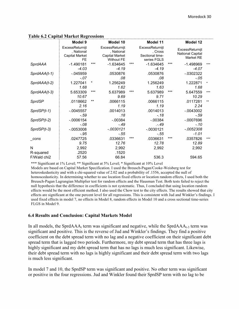
Table 6.2 Capital Market Regressions


ExcessReturnijt, National

Capital Market FE

ExcessReturnijt, National

Capital Market Without FE

ExcessReturnijt, Cross

Sectional time-series FGLS

ExcessReturnijt National Capital

Market RE

SprdAAA -1.490181 *** -1.634645 *** -1.634645 *** -1.498969 ***

-4.03 -4.19 -4.19 -4.07

SprdAAA(t-1) -.045959 .0530876 .0530876 -.0302322

-.07 .08 .08 -.05

SprdAAA(t-2) 1.227041 * 1.256249 1.256249 1.222871 *

1.68 1.62 1.63 1.68

SprdAAA(t-3) 5.653309 *** 5.637989 *** 5.637989 *** 5.647559 ***

10.67 9.69 9.71 10.29

SprdSP .0118662 ** .0066115 .0066115 .0117281 **

2.16 1.19 1.19 2.24

SprdSP(t-1) -.0045557 .0014013 .0014013 -.0043002

-.59 .18 -.18 -.59

SprdSP(t-2) -.0006154 -.00384 -.00384 -.0007696

-.08 -.49 .-.49 -.10

SprdSP(t-3) -.0053008 -.0030121 -.0030121 -.0052308

-.95 -.55 -.55 -1.01

_cons .0247725 .0336631 *** .0336631 *** .0357826 ***

9.75 12.76 12.78 12.89

N 2,992 2,992 2,992 2,992

R-squared .2520 .1520

F/Wald chi2 57.56 66.84 536.3 594.65

6.4 Results and Conclusion: Capital Markets Model

In all models, the SprdAAAt term was significant and negative, while the SprdAAAt-3 term was significant and positive. This is the reverse of Jud and Winkler’s findings. They find a positive coefficient on the debt spread term with no lag and a negative coefficient on their significant debt spread term that is lagged two periods. Furthermore, my debt spread term that has three lags is highly significant and my debt spread term that has no lags is much less significant. Likewise, their debt spread term with no lags is highly significant and their debt spread term with two lags is much less significant. In model 7 and 10, the SprdSP term was significant and positive. No other term was significant or positive in the four regressions. Jud and Winkler found their SprdSP term with no lag to be

*** Significant at 1% Level; ** Significant at 5% Level; * Significant at 10% Level Models are based on Capital Market Specification. I used the Breusch-Pagan/Cooke-Weisberg test for heteroskedasticity and with a chi-squared value of 2.02 and a probability of .1556, accepted the null of homoscedasticity. In determining whether to use location fixed effects or location random effects, I used both the Breusch-Pagan Lagrangian Multiplier test for random effects and the Hausman Test. Both tests failed to reject the null hypothesis that the difference in coefficients is not systematic. Thus, I concluded that using location random effects would be the most efficient method. I also used the Chow test to the city effects. The results showed that city effects are significant at the one percent level for all regressions. This is consistent with Jud and Winkler’s findings. I used fixed effects in model 7, no effects in Model 8, random effects in Model 10 and a cross sectional time-series FLGS in Model 9.

Moredock 31

highly significant, while they found their equity spread term with one lag to be significant to a lesser extent. This implies that as risk premiums increase in the stock market so do risk premiums in real estate. This would suggest efficiency in capital flows. Surprisingly, since the significant SprdSP terms do not have a lag, it suggests that commercial real estate markets show some characteristics of market efficiency. Simply put, during this real estate boom real estate risk premiums moved loosely with stock market risk premiums. That said, the presence of a large and positive coefficient on the SprdAAAt-3 term suggests that commercial real estate markets are still inefficient. Furthermore, the very significant location dummies suggest a lack of integration with national capital markets. My results differ from their study when it comes to R-squared values. My R-squared is only .252 in Model 9. This is relatively small compared to their R-squared value of .8267 for their office regression. I would posit that this is due to the individual transaction nature of my dependent. Whereas their dependent is the semi-annual average of 21 MSAs, mine is 2,992 independent transactions in 12 MSAs. Taking averages across six months and all transactions would allow there to be inner-period adjustment to capital market adjustments. My observation period is smaller and my periods are monthly, thus my dependent has many noticeably different properties than Jud and Winkler’s. Thus, I would argue that my data set is not as well suited for this model. Like the primary and secondary model specifications, the results of the capital market regression suggest that the interest rate of CMBS financing has a tremendous impact on capitalization rates three months into the future. The coefficient of 5.65 implies that a 100 basis point increase in the cost of CMBS financing would force the excess return on real estate up 565 basis points three months into the future. This has extraordinary implications. The constant term was positive and significant in all models.

7 Future Research and Discussion

Given the large impact CMBS debt prices have on cap rates, it is no surprise that very few deals are getting done given current market conditions. In February, the cost of AAA rated debt was higher than the average cap rate. As of February 2008, sales are down year-over-year by 90% as of March for properties worth more than $100 million. This is particularly telling because properties of that size almost always require the use of debt. Wall Street investment banks are

averaging 90-99% less lending activity for 2008 year to date.study would be finding a rate that nearly stops transactions. The recent absence of large transactions suggests there is a rate that will stop almost all transactions that require capital market financing. It would be very interesting to figure it out.

Figure 7.1

99% less lending activity for 2008 year to date.12 An interesting extension of this d be finding a rate that nearly stops transactions. The recent absence of large

transactions suggests there is a rate that will stop almost all transactions that require capital market financing. It would be very interesting to figure it out.

Moredock 32

An interesting extension of this d be finding a rate that nearly stops transactions. The recent absence of large

transactions suggests there is a rate that will stop almost all transactions that require capital
Real Capital Analytics 2008 ©
Likewise, a more broad study of how cand the credit crunch would be enlightening to investors. over the time period of this study only ranged from 60.9 to 132.4sufficient to explain current market conditions. with significant results due to the lack of total transactions and the even greatertransactions using securitized debt financing.

A second interesting extension of this study would be an analysis of how much impact the large influx in capital flows to office properties had during this same time period, from October 2002 to October 2007. Roughly $654 billion poured into net office investment from 2001 to the beginning of 2008. More than $1.5 trillion in commercial real estate properties transactions occurred during these seven years. Figure 7.2

12 Real Capital Analytics. “Quarter in Review: By any Metric Q1 Sales Activity Disappoints.” Monthly. April 2008. 13 Real Capital Analytics, “RCA Net Investment.” March 2008. Online.

of how cap rates are affected by irrational interest rate behavior would be enlightening to investors. Since the spread for CMBS financing this study only ranged from 60.9 to 132.4 basis points, this study is not

sufficient to explain current market conditions. There would be serious difficulties in coming up with significant results due to the lack of total transactions and the even greater lack of transactions using securitized debt financing.

A second interesting extension of this study would be an analysis of how much impact the large influx in capital flows to office properties had during this same time period, from October 2002

ber 2007. Roughly $654 billion poured into net office investment from 2001 to the More than $1.5 trillion in commercial real estate properties transactions

occurred during these seven years. 13

Real Capital Analytics. “Quarter in Review: By any Metric Q1 Sales Activity Disappoints.” Capital Trends

Real Capital Analytics, “RCA Net Investment.” March 2008. Online. www.rcanalytics.com

irrational interest rate behavior Since the spread for CMBS financing

this study is not serious difficulties in coming up

lack of

A second interesting extension of this study would be an analysis of how much impact the large influx in capital flows to office properties had during this same time period, from October 2002

ber 2007. Roughly $654 billion poured into net office investment from 2001 to the More than $1.5 trillion in commercial real estate properties transactions

Capital Trends

http://www.rcanalytics.com/

Large capital inflows may be attributed to the falling dollar, the health of the U.S. economy, the preference for stable returns, the creation of wealth, the desirability of U.S. office buildings, or the ease of acquiring debt against U.S. commercial real has fallen, marginal labor has becomepresences in the United States. Speculation supply-constrained markets like New York, DC, and San Francisco where barriers to development are high and long run occupancy is high. Furthermore, due to the heterogeneity and depth of their economies, office buildings with specific uses, such as biotech or stock trading, are more easily substitutable amongst local businesses. Looking forward, the outlook for commercial real estate is not particularly brightlarge increase in investment. In fact, recent reports from the research departments at J.P. Morgan Securities and Goldman Sachs are predicting 20 percent and 26 percent declines peak to trough respectively.14 January and February transaction volume comparison to $68 billion a year before.storm. Distressed funds are flush with cash and waiting for highly leveraged properties to not cover rent. In predicting where prices will resettle, we can look at CMBS spreaExperts predict that spreads will perlong run rate of AAA 5 year debt goes up cap rates of a quarter point given this study’s optimal model. If the spread suffers a permanent increase of 20 basis points, we can expect average cap rates to increase half a percentage. Similarly, if we use the national capital market model, we may see a half percentage or full percentage increase in long run average cap rates. Only time will tell, but afsafe to confirm the proverbial industry

14 Hudgins, Matt. National Real Estate Investor, “Shrinking Values, Growing Anxiety.” April 1, 2008.

Large capital inflows may be attributed to the falling dollar, the health of the U.S. economy, the the creation of wealth, the desirability of U.S. office buildings, or

against U.S. commercial real estate to outsize returns. has fallen, marginal labor has become cheaper, potentially causing multi-nationals to grow their

Speculation may be partially responsible as well, especially in kets like New York, DC, and San Francisco where barriers to

development are high and long run occupancy is high. Furthermore, due to the heterogeneity and depth of their economies, office buildings with specific uses, such as biotech or stock trading, are more easily substitutable amongst local businesses.

he outlook for commercial real estate is not particularly bright. In fact, recent reports from the research departments at J.P. Morgan

es and Goldman Sachs are predicting 20 percent and 26 percent declines peak to trough January and February transaction volume was only $6.8 billion, which is paltry in $68 billion a year before. There is a very real sense that this is the calm before the

storm. Distressed funds are flush with cash and waiting for highly leveraged properties to not In predicting where prices will resettle, we can look at CMBS spreads for AAA debt.

spreads will permanently widen in the long run. If that means the median long run rate of AAA 5 year debt goes up 10 basis points, we should see an increase in average cap rates of a quarter point given this study’s optimal model. If the spread suffers a permanent

e of 20 basis points, we can expect average cap rates to increase half a percentage. Similarly, if we use the national capital market model, we may see a half percentage or full percentage increase in long run average cap rates. Only time will tell, but after this study, isafe to confirm the proverbial industry saying, “It’s all about the spread.”

Hudgins, Matt. National Real Estate Investor, “Shrinking Values, Growing Anxiety.” April 1, 2008.

Moredock 33

Large capital inflows may be attributed to the falling dollar, the health of the U.S. economy, the the creation of wealth, the desirability of U.S. office buildings, or

to outsize returns. As the dollar nationals to grow their

may be partially responsible as well, especially in kets like New York, DC, and San Francisco where barriers to

development are high and long run occupancy is high. Furthermore, due to the heterogeneity and depth of their economies, office buildings with specific uses, such as biotech or stock trading, are

he outlook for commercial real estate is not particularly bright despite the . In fact, recent reports from the research departments at J.P. Morgan

es and Goldman Sachs are predicting 20 percent and 26 percent declines peak to trough billion, which is paltry in this is the calm before the

storm. Distressed funds are flush with cash and waiting for highly leveraged properties to not ds for AAA debt.

. If that means the median 10 basis points, we should see an increase in average

cap rates of a quarter point given this study’s optimal model. If the spread suffers a permanent e of 20 basis points, we can expect average cap rates to increase half a percentage.

Similarly, if we use the national capital market model, we may see a half percentage or full ter this study, it is

Hudgins, Matt. National Real Estate Investor, “Shrinking Values, Growing Anxiety.” April 1, 2008.

7 Appendix

Figure 1: As interest rates have declined, prices have moved upwards, showing an inverse relationship.

: As interest rates have declined, prices have moved upwards, showing an inverse relationship.

Moredock 34

: As interest rates have declined, prices have moved upwards, showing an inverse relationship.

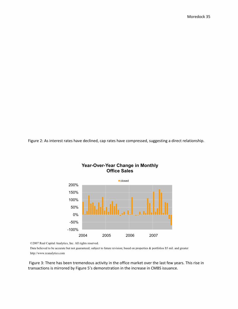
Figure 2: As interest rates have declined, cap rates have compressed, suggesting a direct relationship.


Data believed to be accurate but not guaranteed; subject to future revision; based on properties & portfolios $5 mil. and


Figure 3: There has been tremendous activity in the office market over the last few years. This rise in

transactions is mirrored by Figure 5’s demonstration in the increase in CMBS issuance.

-100%

-50%

0%

50%

100%

150%

200%

2004

Year

declined, cap rates have compressed, suggesting a direct relationship.


Data believed to be accurate but not guaranteed; subject to future revision; based on properties & portfolios $5 mil. and

: There has been tremendous activity in the office market over the last few years. This rise in

transactions is mirrored by Figure 5’s demonstration in the increase in CMBS issuance.

2005 2006 2007

Year-Over-Year Change in Monthly Office Sales

closed

Moredock 35

declined, cap rates have compressed, suggesting a direct relationship.


: There has been tremendous activity in the office market over the last few years. This rise in

©2007 Real Capital Analytics, Inc. All rights reserved. Data believed to be accurate but not guaranteed; subject to future revision; based on properties & portfolios $5 mil. and grehttp://www.rcanalytics.com

Figure 4: Office financing is procured through traditional lending, such as direct lending, in addition to CMBS financing.


Cap Rate Spread To Treasuries

in basis points


Data believed to be accurate but not guaranteed; subject to future revision; based on properties & portfolios $5 mil. and gre


Figure 5: Demonstration of the mispricing of risk, or the revaluation of commercial real estate risk by the

markets.

-

100

200

300

400

500

2004

percent of Office Buyers

Financed by CMBS

©2007 Real Capital Analytics, Inc. All rights reserved. Data believed to be accurate but not guaranteed; subject to future revision; based on properties & portfolios $5 mil. and gre

: Office financing is procured through traditional lending, such as direct lending, in addition to



Data believed to be accurate but not guaranteed; subject to future revision; based on properties & portfolios $5 mil. and gre

the mispricing of risk, or the revaluation of commercial real estate risk by the

2004 2005 2006 2007

Office - CBDOffice - Sub

Moredock 36


: Office financing is procured through traditional lending, such as direct lending, in addition to


the mispricing of risk, or the revaluation of commercial real estate risk by the


Moredock 37




Figure 6: After the credit crunch, a shift occurred in office purchasers. This shift is indicative of financial

sponsors’ need for leverage. This purchaser mix is more sustainable with tighter capital markets.

18%

8%

13%

3%

30%

3%

0%

16%

9%

Office Jan-Aug 07

22%

17%

3%

4%

12%10%

1%

20%

12%

Office Sept - Date07

mid high/rise Jan-Aug 07inst'l foreign reit/public

user/other fund syndicator

condo converter pvt in state pvt out of state

Mo

red

ock

38

Year Built

Mean

Std Error

Median

Mode

Std Dev

Variance

Kurtosis

Skewn

Range

Min

Max

NYC

1934

1.43

1926

1925

30.20

9.12E+02

(0.02)

0.40

195

1810

2005

Boston

1962

2.57

1980

1985

39.41

1.55E+03

0.05

(1.06)

193

1814

2007

Chicago

1970

1.91

1981

1986

32.51

1.06E+03

0.01

(1.11)

125

1881

2006

National

1973

0.57

1984

1985

31.09

9.66E+02

1.00

(1.34)

197

1810

2007

SF

1974

1.42

1984

2001

30.27

9.16E+02

0.96

(1.39)

153

1853

2006

Minneapolis

1977

2.78

1984

1985

25.94

6.73E+02

4.13

(1.99)

121

1885

2006

KC

1983

3.16

1985

1977

22.36

5.00E+02

10.50

(2.78)

126

1880

2006

DC

1982

0.74

1986

1987

20.63

4.25E+02

6.39

(2.12)

157

1850

2007

Dallas

1988

0.82

1986

1985

14.06

1.98E+02

8.42

(2.01)

101

1905

2006

Atlanta

1987

1.02

1987

1985

16.31

2.66E+02

8.31

(2.39)

108

1898

2006

Nashville

1985

2.77

1988

2000

19.17

3.68E+02

6.06

(2.08)

101

1906

2007

Denver

1988

1.34

1994

2001

17.15

2.94E+02

6.67

(2.13)

101

1906

2007

Charlotte

1989

1.80

1997

1999

17.34

3.01E+02

2.93

(1.56)

80

1926

2006

SqFt/Building

Mean

Std Error

Median

Mode

Std Dev

Variance

Kurtosis

Skewn

Range

Min

Max

NYC

447,465

24384

255,180

380,000

516,110

2.66E+11

5.35

2.16

2,941,516

130

2,941,646

Minneapolis

285,514

28868

190,008

359,540

270,807

7.33E+10

2.92

1.67

1,365,994

24,900

1,390,894

Chicago

357,223

30874

156,055

232,000

532,963

2.84E+11

14.07

3.31

3,786,841

397

3,787,238

National

252,626

6225

134,924

100,000

343,249

1.18E+11

21.28

3.86

3,787,153

85

3,787,238

DC

182,130

6001

128,475

108,000

167,802

2.82E+10

9.70

2.52

1,375,039

190

1,375,229

Dallas

227,101

16592

126,203

100,000

285,458

8.15E+10

10.17

3.02

1,738,915

85

1,739,000

Atlanta

211,207

15161

121,828

64,574

243,995

5.95E+10

33.97

4.46

2,527,395

17,900

2,545,295

Boston

261,817

24764

119,168

150,000

381,232

1.45E+11

19.49

3.79

2,884,707

293

2,885,000

Nashville

147,329

14764

117,645

312,297

102,287

1.05E+10

(0.44)

0.74

386,581

24,000

410,581

Denver

183,420

17045

111,911

488,640

217,620

4.74E+10

11.88

3.20

1,270,195

21,928

1,292,123

KC

185,997

43690

111,088

#N/A

312,006

9.73E+10

36.14

5.69

2,176,970

23,030

2,200,000

Charlotte

159,345

15841

105,497

37,800

153,583

2.36E+10

5.78

2.25

863,093

23,987

887,080

SF

184,347

10492

104,862

189,000

226,484

5.13E+10

15.68

3.30

1,791,943

8,057

1,800,000

Occupancy

Mean

Std Error

Median

Mode

Std Dev

Variance

Kurtosis

Skewn

Range

Min

Max

KC

93.6%

0.0133

99.0%

10.095

8.97E-03

2.10

(1.65)

0.36

0.64

1

DC

93.5%

0.0048

99.0%

10.133

1.77E-02

25.60

(4.54)

10

1

National

91.6%

0.0026

97.0%

10.144

2.07E-02

18.51

(3.79)

10

1

SF

90.8%

0.0079

97.5%

10.162

2.61E-02

11.97

(3.15)

10

1

Charlotte

92.0%

0.0133

97.0%

10.123

1.50E-02

6.79

(2.48)

0.63

0.37

1

Boston

93.7%

0.0076

97.0%

10.114

1.30E-02

35.52

(5.01)

10

1

NYC

91.9%

0.0078

97.0%

10.161

2.60E-02

21.44

(4.39)

10

1

Chicago

90.8%

0.0076

94.0%

10.127

1.61E-02

18.57

(3.46)

10

1

Denver

92.0%

0.0070

94.0%

10.087

7.59E-03

0.20

(0.98)

0.35

0.65

1

Dallas

89.1%

0.0101

94.0%

10.168

2.82E-02

11.58

(3.09)

10

1

Nashville

88.9%

0.0292

94.0%

10.200

4.02E-02

12.94

(3.50)

10

1

Minneapolis

90.0%

0.0150

93.0%

10.135

1.83E-02

23.86

(3.91)

10

1

Atlanta

88.5%

0.0095

92.0%

10.149

2.21E-02

11.96

(2.87)

10

1

Mo

red

ock

39

Close Price

Mean

Std Error

Median

Mode

Std Dev

Variance

Kurtosis

Skewn

Range

Min

Max

Sum

Count

Conf(95.0%)

NYC

212,275,704

15,029,757

91,400,000

70,000,000

318,119,987

1.01E+17

10.94

3.05

2,234,400,000

5,600,000

2,240,000,000

95,099,515,363

448

29,537,758

DC

55,556,140

2,563,996

28,100,000

23,000,000

71,700,250

5.14E+15

16.66

3.40

668,000,000

0668,000,000

43,444,901,631

782

5,033,139

National

74,949,663

2,879,953

25,000,000

-

158,789,647

2.52E+16

48.80

5.99

2,240,000,000

02,240,000,000

227,846,974,160

3,040

5,646,853

SF

55,634,245

4,464,085

24,500,000

-

96,366,358

9.29E+15

43.14

5.51

1,050,000,000

01,050,000,000

25,925,558,123

466

8,772,279

Boston

82,951,044

10,704,069

22,500,000

6,000,000

164,787,049

2.72E+16

15.03

3.65

1,160,000,000

01,160,000,000

19,659,397,533

237

21,087,731

Chicago

73,353,653

7,997,456

21,900,000

8,500,000

138,057,498

1.91E+16

23.92

4.20

1,214,975,000

5,025,000

1,220,000,000

21,859,388,696

298

15,738,861

Minneapolis

38,777,304

4,878,461

20,991,956

5,000,000

45,764,025

2.09E+15

7.10

2.54

240,000,000

5,000,000

245,000,000

3,412,402,718

889,696,470

Charlotte

24,780,047

2,822,348

17,825,000

46,500,000

27,363,675

7.49E+14

16.78

3.59

189,100,000

5,000,000

194,100,000

2,329,324,417

945,604,623

Denver

31,751,256

4,126,617

15,800,000

6,900,000

52,685,121

2.78E+15

20.26

4.27

340,000,000

5,000,000

345,000,000

5,175,454,732

163

8,148,896

Atlanta

35,325,045

2,929,343

15,700,000

8,500,000

47,143,308

2.22E+15

22.10

3.73

432,192,256

0432,192,256

9,149,186,646

259

5,768,465

Dallas

28,714,303

2,321,284

15,075,000

-

39,936,887

1.59E+15

16.48

3.58

318,000,000

0318,000,000

8,499,433,626

296

4,568,376

KC

24,043,146

5,613,641

13,350,000

17,500,000

40,089,416

1.61E+15

35.44

5.59

281,750,000

0281,750,000

1,226,200,450

5111,275,330

Nashville

18,685,837

2,422,840

12,250,000

9,750,000

16,785,931

2.82E+14

3.44

1.91

73,000,000

5,250,000

78,250,000

896,920,193

484,874,126

$/Sq

ftMean

Std Error

Median

Mode

Std Dev

Variance

Kurtosis

Skewn

Range

Min

Max

Sum

Count

Conf(95.0%)

NYC

948.1

491.9307626

380.0

380.0

10,412.21

1.08E+08

447.41

21.15

220670

99220769

424761

448

966.78

SF

279.9

6.308276944

249.5

223.0

136.18

1.85E+04

3.11

1.37

989

0989

130453

466

12.40

DC

794.5

524.6448392

239.5

230.0

14,671.31

2.15E+08

781.88

27.96

410526

0410526

621289

782

1029.88

Boston

2,674.1

2426.937009

213.0

235.0

37,362.22

1.40E+09

236.99

15.39

575427

0575427

633763

237

4781.23

National

718.0

248.5597964

205.5

0.0

13,704.64

1.88E+08

1,304.88

34.78

575427

0575427

2182678

3,040

487.36

Charlotte

167.9

5.83329314

167.0

170.0

56.56

3.20E+03

0.53

0.35

297

46343

15787

9411.58

Chicago

490.3

317.69

164.5

127.0

5,484.11

3.01E+07

297.91

17.26

94785

5194836

146095

298

625.20

Denver

161.8

5.358351134

149.0

149.0

68.41

4.68E+03

1.18

1.08

354

45399

26368

163

10.58

Atlanta

158.4

3.915172115

145.0

81.0

63.01

3.97E+03

1.27

0.92

407

0407

41016

259

7.71

KC

139.4

8.147407793

138.0

154.0

58.18

3.39E+03

1.68

0.35

334

0334

7107

5116.36

Nashville

135.6

8.362068697

128.0

92.0

57.93

3.36E+03

0.79

0.81

278

40318

6511

4816.82

Minneapolis

142.1

8.378646632

126.0

75.0

78.60

6.18E+03

7.84

2.50

448

53501

12508

8816.65

Dallas

547.4

408.9357486

124.0

0.0

7,035.60

4.95E+07

295.93

17.20

121176

0121176

162030

296

804.80

Cap Rate

Mean

Std Error

Median

Mode

Std Dev

Variance

Kurtosis

Skewn

Range

Min

Max

Sum

Count

Conf(95.0%)

NYC

6.2%

0.000654786

6.30%

6.0%

0.01

1.92E-04

0.01

(0.00)

0.079

0.025

0.104

27.977

448

0.0013

SF

7.0%

0.000823821

6.80%

6.0%

0.02

3.16E-04

0.89

0.55

0.112

0.021

0.133

32.547

466

0.0016

DC

7.1%

0.000470471

7.00%

7.0%

0.01

1.73E-04

0.58

0.18

0.098

0.024

0.122

55.727

782

0.0009

National

7.2%

0.000268592

7.10%

7.0%

0.01

2.19E-04

1.03

0.24

0.114

0.02

0.134

218.632

3,040

0.0005

Denver

7.5%

0.001013226

7.30%

7.3%

0.01

1.67E-04

0.96

0.32

0.081

0.03

0.111

12.237

163

0.0020

Boston

7.2%

0.000936016

7.30%

7.3%

0.01

2.08E-04

0.59

0.10

0.087

0.032

0.119

17.114

237

0.0018

Atlanta

7.4%

0.000831912

7.40%

6.4%

0.01

1.79E-04

1.25

0.21

0.095

0.03

0.125

19.248

259

0.0016

Charlotte

7.5%

0.001260165

7.40%

7.3%

0.01

1.49E-04

1.08

0.13

0.075

0.041

0.116

7.08

940.0025

Chicago

7.6%

0.00

7.60%

8.2%

0.01

1.87E-04

1.92

0.37

0.112

0.020

0.132

22.70

298

0.0016

Dallas

7.8%

0.000887967

7.60%

8.0%

0.02

2.33E-04

1.64

0.46

0.109

0.025

0.134

23.003

296

0.0017

KC

7.8%

0.001898849

7.70%

8.0%

0.01

1.84E-04

1.75

0.81

0.072

0.051

0.123

3.957

510.0038

Minneapolis

7.9%

0.001246814

7.75%

7.2%

0.01

1.37E-04

1.54

0.76

0.068

0.051

0.119

6.946

880.0025

Nashville

8.0%

0.001712423

8.00%

8.0%

0.01

1.41E-04

(0.20)

0.18

0.053

0.052

0.105

3.859

480.0034

Mo

red

ock

40

Transaction Type

Mean

Std Error

Median

Mode

Std Dev

Variance

Kurtosis

Skewn

Range

Min

Max

SF

0.682

0.0216

11

0.47

0.22

(1.39)

(0.79)

10

1

Dallas

0.635

0.0280

11

0.48

0.23

(1.69)

(0.56)

10

1

Atlanta

0.629

0.0301

11

0.48

0.23

(1.72)

(0.54)

10

1

Chicago

0.594

0.0285

11

0.49

0.24

(1.86)

(0.38)

10

1

Denver

0.589

0.0387

11

0.49

0.24

(1.89)

(0.36)

10

1

Minneapolis

0.557

0.0533

11

0.50

0.25

(1.99)

(0.23)

10

1

Boston

0.527

0.0325

11

0.50

0.25

(2.00)

(0.11)

10

1

National

0.522

0.0091

11

0.50

0.25

(1.99)

(0.09)

10

1

KC

0.510

0.0707

11

0.50

0.25

(2.08)

(0.04)

10

1

DC

0.506

0.0179

11

0.50

0.25

(2.00)

(0.03)

10

1

Charlotte

0.457

0.0517

00

0.50

0.25

(2.01)

0.17

10

1

Nashville

0.438

0.0724

00

0.50

0.25

(2.02)

0.26

10

1

NYC

0.375

0.0229

00

0.48

0.23

(1.74)

0.52

10

1

Moredock 1

1

8 Works Cited

Ambrose, B. and H. Nourse (1993) Factors Influencing Capitalization Rates. Journal of Real Estate Research 8, 221-237. Brueggeman, William B., and Jeffrey .D. Fisher (2006) Real Estate Finance and Investments. (13th edition) McGraw-Hill: New York. Fisher, J., G. Lentz, and J. Stern (1984) Tax Incentives for Investment in Nonresidential Real Estate. National Tax Journal. 37, 69-87. Froland, C. (1987) What Determines Cap Rates on Real Estate, Journal of Portfolio Management, 13, 77-83. Giliberto, M. (1996) Commercial Real Estate Annual Review and Outlook, Lehman Brothers, Inc. Hardin III, William, Kartono Liano and Kam Chan (2006) Influential Journals, Institutions and Researchers in Real Estate. Real Estate Economics, vol 34, 457-478. Hartzell, D., J. Hekman, and M. Miles (1987) Diversification Categories in Investment Real Estate. AREUEA Journal, 15, 98-109. Hendershott, P.H. (1996) Valuing Properties When Comparable Sales Do Not Exist and the Market is in Disequilibrium. Journal of Property Research, 13, 57-61. Hendershott, P.H., and Bengt Turner (1998) Estimating constant-quality capitalization rates and capitalization effects of below market financing. Journal of Property Research, 16(2), 109-122. Hudgins, Matt. National Real Estate Investor, “Shrinking Values, Growing Anxiety.” April 1, 2008. Jud, D., and D. Winkler (1995) The Capitalization Rate of Commercial Properties and Market Returns. Journal of Real Estate Research. 10, 509-518. Korpacz (1996) Real Estate Investment Survey, 2nd Quarter. Real Capital Analytics. All sources can be found online. www.rcanalytics.com


Moredock 2

2

Sivitanidou, Rena and Petros Sivitanides (1999) Office Capitalization Rates: Real Estate and Capital Market Influences. Journal of Real Estate Finance and Economics, 18:3, 297-322.

office capitalization rates: the effects of interest rates · office capitalization rates: the...

Documents