By Hui Bian

Office for Faculty Excellence

1

• My office is located in 1001 Joyner library, room 1006

• Email: bianh@ecu.edu

• Tel: 252-328-5428

• You can download sample data files from: http://core.ecu.edu/ofe/StatisticsResearch/

2

• What is bivariate relationship?

–The relationship of two measures/variables.

–The direction of the relationship

–The strength of the relationship

–Whether the relationship is statistically significant

• Measures of association—a single summarizing number that reflects the strength of the relationship. This statistic shows the magnitude and/or direction of a relationship between variables.

• Magnitude—the closer to the absolute value of 1, the stronger the association. If the measure equals 0, there is no relationship between the two variables.

• Direction—the sign on the measure indicates if the relationship is positive or negative. In a positive relationship, when one variable is high, so is the other. In a negative relationship, when one variable is high, the other is low.

• Measurement

• Nominal: Numbers that are simply used as identifiers or names represent a nominal scale of measurement such as female vs. male.

• Ordinal: An ordinal scale of measurement represents an ordered series of relationships or rank order. Likert-type scales (such as "On a scale of 1 to 10, with one being no pain and ten being high pain, how much pain are you in today?") represent ordinal data.

• Interval: A scale that represents quantity and has equal units but for which zero represents simply an additional point of measurement is an interval scale. The Fahrenheit scale is a clear example of the interval scale of measurement. Thus, 60 degree Fahrenheit or -10 degrees Fahrenheit represent interval data.

• Ratio: The ratio scale of measurement is similar to the interval scale in that it also represents quantity and has equality of units. However, this scale also has an absolute zero (no numbers exist below zero). For example, height and weight.

• Relationship based on measurement

–Two scale variables (two quantitative variables)

–Two categorical variables (nominal or ordinal)

–One categorical and one scale variable

• Statistical analyses for testing relationships between two quantitative variables

–Correlation

–Linear regression

• Pearson Correlation r –Measures linear association –It is the standardized regression

coefficient (doesn’t depend on variables’ units)

–It is between -1 and +1 –The larger the absolute value of r, the

strongly the degree of linear association

• Pearson Correlation r

–Pearson’s correlation coefficient assumes that each pair of variables is bivariate normal.

–There is no causal relationship between two variables.

• Example: we want to know the correlation between height and weight.

–Step 1: check the linear relationship between two variables using Scatter plot.

–Step 2: use Bivariate correlation to get Pearson correlation.

• In SPSS, got to Graphs > Chart Builder

• Pearson correlation r: go to Analyze > Correlate > Bivariate

• SPSS output

• Use Linear regression to test the relationship between weight and height.

–We want to use height to predict weight .

• Regression Equation

– Ypredicted = a + bx

Ypredicted : predicted score of dependent variable X: predictor a: intercept b: slope/regression coefficient

• Regression line

Y

X

Regression line

Intercept

Slope 0

• Residuals

–The difference between observed and predicted values of the dependent variable.

–We use residuals to check the goodness of the prediction equation.

• Least square – We use Least Square Criterion to estimate parameters.

– Lease Square means the sum of the squared estimated errors of predictions is minimized.

The line best fits the data. The vertical distance between observed values of y and line is the residual. Residuals or errors =

y(observed score- predicted score)

• Simple linear regression

–Go to Analyze > Regression > Linear

• Click Statistics and click Plots

• SPSS output

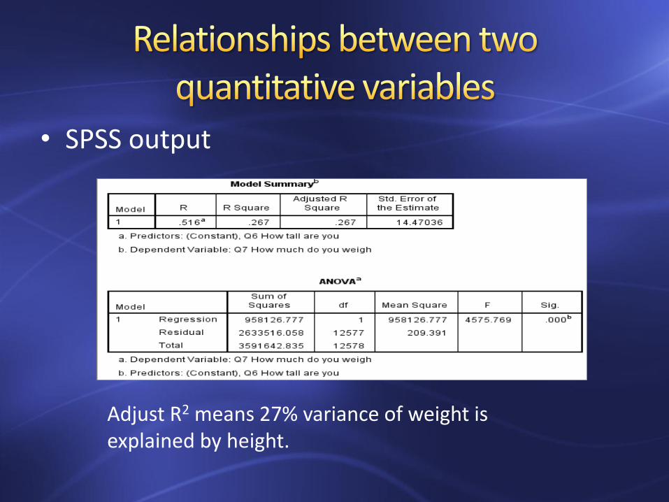
• SPSS output

Adjust R2 means 27% variance of weight is explained by height.

• SPSS output

• SPSS output: distribution of residuals

• Statistical analyses for testing relationships between two categorical variables

–Contingency tables(Crosstabs)

–Correlation

–Regression: linear, logistic regression, ordinal, and multinominal regression

• Crosstabs in SPSS: “Crosstabs procedure offers tests of independence and measures of association and agreement for nominal and ordinal data. “

• From SPSS, a bunch of tests are used to test association

• Chi-square: for two by two table and For tables with any number of rows and columns. – It measures the discrepancy between the

observed cell counts and what expected if the rows and columns were unrelated.

• Fisher’s exact test: for tables that have a cell with an expected frequency of less than 5.

• Example: we want to know if that the number of drug (Drgu_N) use is associated with sex (Q2).

• Go to Analyze > Descriptive Statistics > Crosstabs

• Click Statistics

• Click Cells

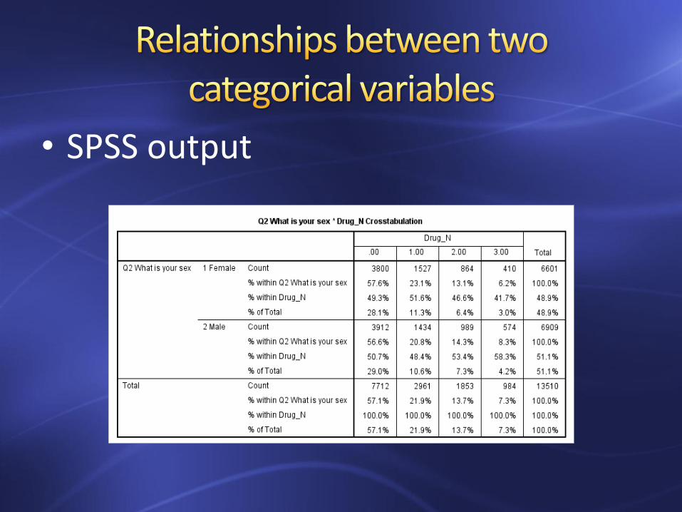
• SPSS output

• SPSS output: bar chart

• Results

–Look at the percentages within grade

P = .00 < 0.05, so there is a significant association between sex and number of drug use.

• Correlation –Pearson correlation coefficient: for

quantitative, normally distributed variables.

• Kendall’s tau-b or Spearman: for data are NOT normally distributed or have ordered categories. it is a nonparametric statistic.

• Spearman's rank-order correlation: measures the strength of association between two ranked variables.

• Example: we want to measure correlation between drinking (Q43) and marijuana use (Q49)

• Go to Analyze > Correlate > Bivariate

• SPSS output

• Logistic regression

–Dependent variable: one dichotomous/binary variable

–Independent variables: continuous or categorical

• The goal of logistic regression is to determine the probability of a case belonging to the 1 category of dependent variable or the probability of event occurring (event occurring is always coded as 1) for a given set of predictors.

48

The Y-axis is P (probability), which indicates the proportion of 1s at any given value of X.

• Logistic regression equation – log(p/1-p) = a + bx – Logit (p) = a + bx

p: probability of a case belonging to category 1

p/1-p: odds a: constant b: regression coefficient, about whether p

increases/decreases as x increases

• Odds

Odds of Success = Probability of Success/Probability of failure

If Probability of Success = .75, then the probability of failure = 1 - .75=.25, then odds of Success = .75/.25 =3

• Odds

–Odds of Success > 1 means a success is more likely than a failure.

–Odds of Success < 1 means a success is less likely than a failure

• Odds ratio is the ratio of odds

• Example: we want to know the association between Ever feel sad or hopeless (Q26r) (independent variable) and marijuana use (Q49r) (Dependent variable)

• Contingency table

• Q49r is our dependent variable, in another word, we want to know the probability of using marijuana (Use group and coded as 1).

• The probability of a student using marijuana is 3998/13242=.302

• We want to know whether this proportion is the same for all levels of Sad group.

• Odds of a Sad student using marijuana = 1345/2653 = .51

• Odds of a Happy student using marijuana = 1999/7245 = .28

• Odds ratio of using marijuana between Sad and Happy students = .51/.28 = 1.82 ( Happy group is the reference category)

• Logistic regression

• Go to Analyze > Regression >Binary Logistic

• Click Categorical: No group is the reference

Check First as Reference category and click Change

• Click Options

• SPSS output

The coding table is very important for understanding the results. The column of Parameter coding is the coding used in data analysis which matches with our coding of variable Q26r. We want them to match so that we don’t have our minds boggle when interpret results.

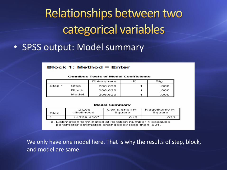
• SPSS output: Model summary

We only have one model here. That is why the results of step, block, and model are same.

• SPSS output

Q26r is a significant predictor. B value is positive, which means there is a positive relationship between feelings and marijuana use. Exp (B) is odds ratio, which means people who felt sad and hopeless 1.84 times more likely used marijuana than people who didn’t have that kind of feelings.

• Statistical analyses for testing relationships between one categorical variable and one scale variables

–Correlation

–T test, ANOVA

–Regression

• Test means: t tests and Analysis of variance

– T tests

• one sample t test

• Independent-samples t test

• Paired-samples t test

– Analysis of variance (ANOVA)

• One-way/two-way between subject design

• One-way/two-way within subject design

• Mixed design

• Go to Analyze > Compare Means

• Student’s T test – The method assumes that the results follow the

normal distribution (also called student's t-distribution) if the null hypothesis is true.

– The paired t-test is used when you have a paired design.

– The independent t-test is used when you have an independent design.

• Independent-samples t test – Example: we want to know if there is a

difference between sex groups (Q2) in height (Q6).

–Go to Analyze > Compare Means > Independent-Samples T Test

• Test variable: Q6 (dependent variable)

• Grouping variable: Q2 (two groups: female and male)

• Coding of Q2: 1= Female and 2= Male

Click Define Groups, type 1 for Group 1 and 2 for Group 2 based upon the coding of Q2

• SPSS output

• Mean height of females = 1.62, SD = .07

• Mean height of males = 1.76, SD = .09

• t = -94.28, df = 12470.68, p = .00

• Conclusion: there is significant difference between female and male groups in height.

• Analysis of Variance (ANOVA) –Used to compare means of two or more

than two groups

–One-way ANOVA (between subjects): there is only one factor variable

– Example: we want to know if there is difference in height (Q6) among four grade groups (Q3)

• Original coding of Q3

• We need to recode Q3 in order to get rid of the last category.

–Then the new variable has four categories

–Go to Transform > Recode into a different variable

• Recoding Q3 into Q3r

• Go to Analyze > General Linear Model > Univariate

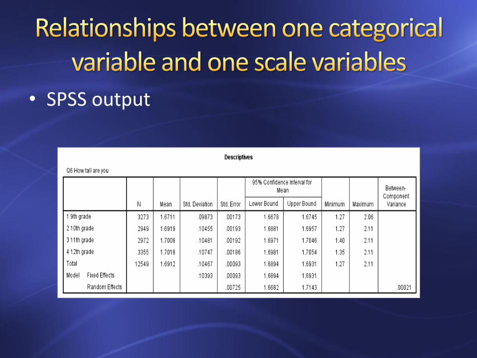
• SPSS output

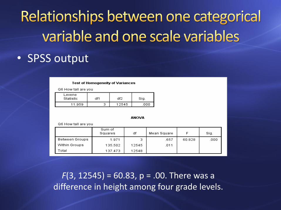
• SPSS output

F(3, 12545) = 60.83, p = .00. There was a difference in height among four grade levels.

• Post Hoc tests

–We have already obtained a significant omnibus F-test with a factor of four levels.

–We need to know which means are significantly different.

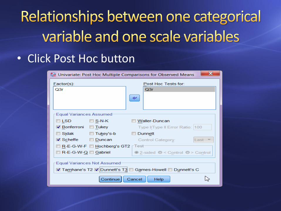
• Click Post Hoc button

• Results of Post Hoc tests

Meyers, L. S., Gamst, G., & Guarino, A. J. (2006). Applied multivariate research: design and interpretation. Thousand Oaks, CA: Sage Publications, Inc.

82