ogor2 satellite - nasa
TRANSCRIPT
?
I
I !
I
1
/
/
PROCESSING OF MAGNETOMETER
/ ’
X -61 2-6 7 - 2 7 2 . .
THE TOTAL FiELD IATA FROM THE
OGOr2 SATELLITE
R. A. LANGEL
.-
GPO PRICE
JUNE 1967 rq 6 7 30 1 4 7
I (ACCESSION NUMBER)
0
* L J2bJ
L. CxvX -K<f32
\ GODDARD SPACE FLIGHT CENTER
- (PAGES) 4 <
(NASA CR OR TMX OR AX NUMBER)
-c GREENBELT, MARY LAND -
(THRU)
I (CATEGORY)
a
X-612-67-272
PROCESSING OF THE TOTAL FIELD
MAGNETOMETER DATA FROM THE
OW-2 SATELLITE
R. A. Langel
June 1967
NASA Goddard Space Flight Center Greenbelt. Maryland
CONTENTS
1 . 2 .
3 . 4 . 5 . 6 . 7 . 8 . 9 .
10 . 11 . 1 2 . 13 . 14 .
Page
I n t r o d u c t i o n . . . . . . . . . . . . . . . . . . . . . . . 1
The S p a c e c r a f t Te lemet ry System . . . . . . . . . . . . . 6
Magnetometer and Assoc ia t ed I n s t r u m e n t a t i o n . . . . . . . 10
Data Reduct ion Before Data Reaches t h e Experimenter . . . 1 2
O u t l i n e of Experimenter Data Reduct ion Procedures . . . . 1 6
C u l l i n g of Suspec t Data . . . . . . . . . . . . . . . . . 1 9
Output From Main P rocesso r . . . . . . . . . . . . . . . . 30
Recovery of Suspec t Data . . . . . . . . . . . . . . . . . 33
A T i m e Ordered Index . . . . . . . . . . . . . . . . . . . 36
Data For Ana lys i s . . . . . . . . . . . . . . . . . . . . 39
Data Q u a l i t y . . . . . . . . . . . . . . . . . . . . . . . 42
Data Ex ten t . . . . . . . . . . . . . . . . . . . . . . . 56
Procedures i n Data P rocess ing . . . . . . . . . . . . . . 56
Discuss ion and Conclusions . . . . . . . . . . . . . . . . 64
Acknowledgments . . . . . . . . . . . . . . . . . . . . . 67
References . . . . . . . . . . . . . . . . . . . . . . . . 68
Appendix . . . . . . . . . . . . . . . . . . . . . . . . . 70
-
1
2
3
4
5
6
1. INTRODUCTION
On October 14, 1965, OGO-2, the first of three planned Polar Orbiting
Geophysical Observatories, was launched into an orbit with the following
characteristics:
Inclination 87.4"
Perigee 413 Km
Apogee 1510 Km
Anomalistic Period 104.3 Minutes
OGO-2 is an extremely versatile second generation satellite capable of high bit
rates possessing an on-board tape recorder and, until 10 days after launch
having complete attitude control. It is a "street car" o r observatory type
satellite with a complement of twenty experiments measuring many different
geophysical phenomena as can be seen from the following list of experiments
(S-50 Experiment Bulletin No. 18; Ludwig, 19G6).
Exp. No. Experimenter Organization Experiment Description
Haddock U. Michigan Radio Astronomy measurements at 2.5 and 3.0 mc/s.
Helliwell Stanford U. VLF measurements in the frequency range .2-100 Kc.
Morgan and Dartmouth Study of VLF emissions and whistlers Laaspere between .5 and 10 Kc.
(Experiment Number Not Used)
Holzer and UCLA and Investigation of magnetic field fluctua- Smith J PL tions in the low audio frequency range
using a search coil magnetometer.
Heppner, GSFC Measurement of earth's magnetic field Cain, and Far thing fluctuations.
and associated long period ( > 2 cps)
1
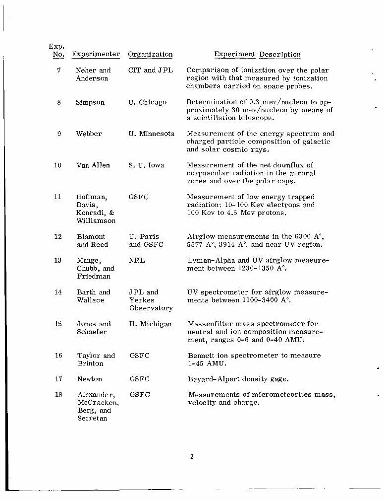
Exp. - No. Experimenter Organization Experiment Description
7 Neher and CIT and J P L Anderson
8 Simpson U. Chicago
9 Webber U. Minnesota
10 Van Allen S. U. Iowa
11 Hoffman, GSFC Davis, Konradi, & Williams on
12 Blamont U. Paris and Reed and GSFC
13 Mange, NRL Chubb, and Friedman
14 Barth and JPL and Wallace Yerkes
Observatory
15 Jones and U. Michigan Schaef er
16 Taylor and GSFC Brinton
17 Newton GSFC
18 Alexander, GSFC McCracken, Berg, and Secretan
Comparison of ionization over the polar region with that measured by ionization chambers carried on space probes.
Determination of 0.3 mev/nucleon to a p proximately 30 mev/nucleon by means of a scintillation telescope.
Measurement of the energy spectrum and charged particle composition of galactic and solar cosmic rays.
Measurement of the net downflux of corpuscular radiation in the auroral zones and over the polar caps.
Measurement of low energy trapped radiation; 10-100 Kev electrons and 100 Kev to 4.5 Mev protons.
Airglow measurements in the 6300 A", 5577 A", 3914 A", and near UV region.
Lyman- Alpha and UV airglow measure- ment between 1230-1350 A".
UV spectrometer for airglow measure- ments between 1100-3400 A".
Massenfilter mass spectrometer for neutral and ion composition measure- ment, ranges 0-6 and 0-40 AMU.
Bennett ion spectrometer to measure 1-45 AMU.
Bay ard- Alpert density gage.
Measurements of micrometeorites mass, velocity and charge.
2
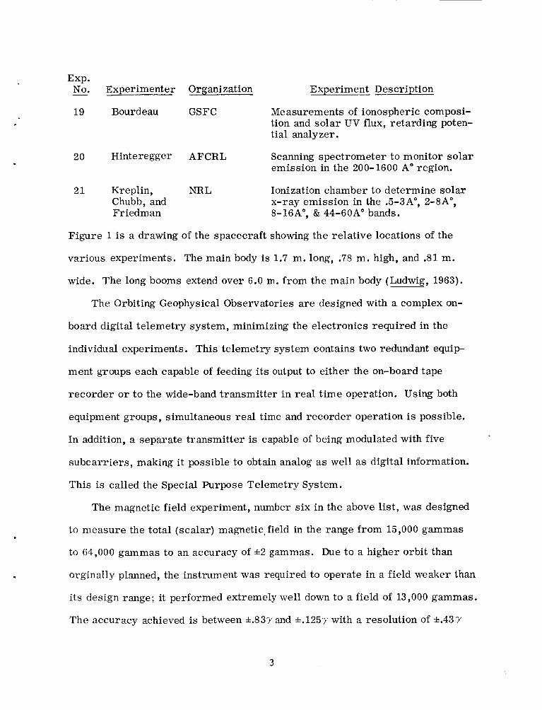
Exp. NO.
19
-
20
21
Experimenter Organization
Bour d e au GSFC
Hinteregger AFCRL
Kreplin, NRL Chubb, and Friedman
Experiment Description
Measurements of ionospheric composi- tion and solar UV flux, retarding poten- tial analyzer.
Scanning spectrometer to monitor solar emission in the 200-1600 A" region.
Ionization chamber to determine solar x-ray emission in the .5-3Ao, 2-8Ao, 8-16Ao, & 44-60A" bands.
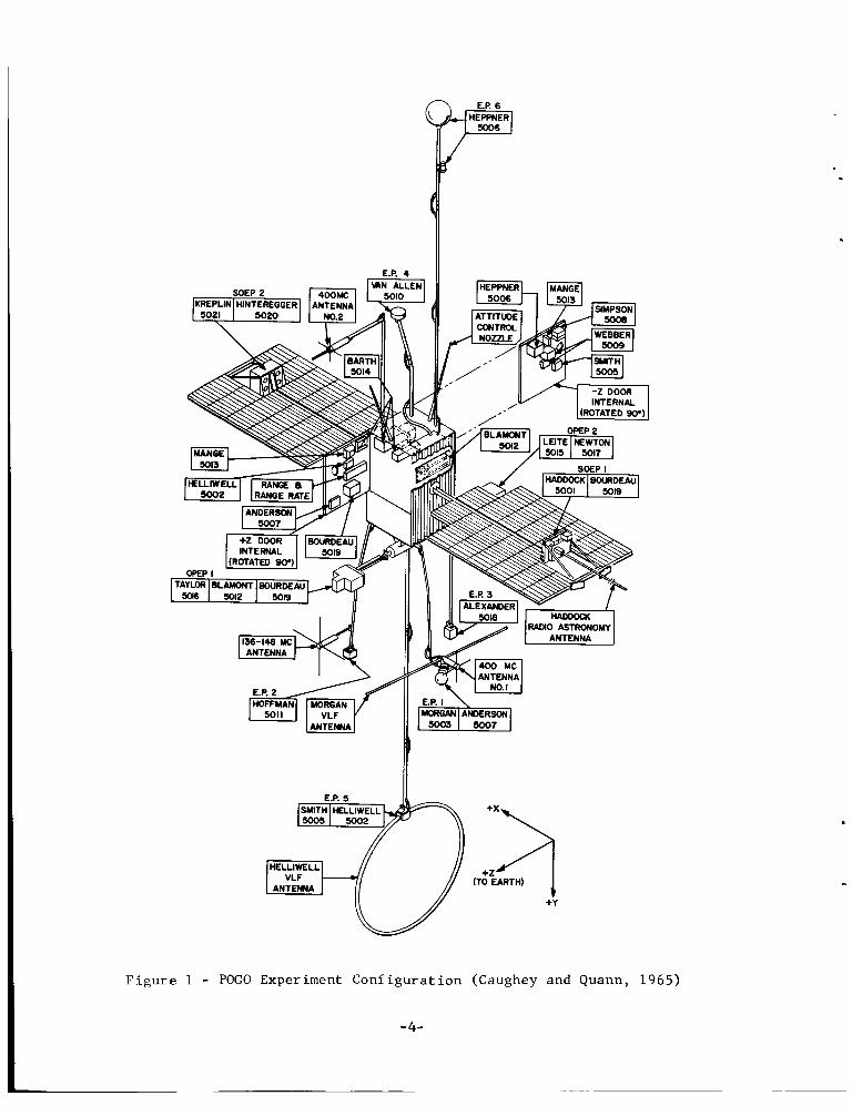
Figure 1 is a drawing of the spacecraft showing the relative locations of the
various experiments. The main body is 1.7 m. long, .78 m. high, and .81 m.
wide. The long booms extend over 6.0 m. from the main body (Ludwig, 1963).
The Orbiting Geophysical Observatories are designed with a complex on-
board digital telemetry system, minimizing the electronics required in the
individual experiments. This telemetry system contains two redundant equip-
ment groups each capable of feeding i ts output to either the on-board tape
recorder o r to the wide-band transmitter in real time operation. Using both
equipment groups , simultaneous real time and recorder operation is possible.
In addition, a separate transmitter is capable of being modulated with five
subcarriers, making it possible to obtain analog as well as digital information.
This is called the Special Purpose Telemetry System.
The magnetic field experiment, number six in the above list, was designed
to measure the total (scalar) magnetic. field in the range from 15,000 gammas
to 64,000 gammas to an accuracy of +2 gammas. Due to a higher orbit than
orginally planned, the instrument was required to operate in a field weaker than
its design range; it performed extremely well down to a field of 13,000 gammas.
The accuracy achieved is between r t . 8 3 ~ and *.125y with a resolution of L43Y
3
E.P. 5 SMITH HELLIWELL 5005 5002
(TO EARTH)
HELLIWELL VLF
ANTEWA +Y
F i g u r e 1 - POGO Experiment C o n f i g u r a t i o n (Caughey and Quann, 1965)
- 4-
(Farthing and Folz, 1966). Since this experiment measures the scalar field and
not the vector field, the data were unaffected by the loss of attitude control early
in the lifetime of the satellite (Cain, Langel, and Hendricks, July 1966). The
instrument performed flawlessly from launch until early July when the failure
of a power supply caused loss of the special purpose telemetry and partial loss
of the digital PCM data (Farthing and Folz, 1966). The extent of the data cov-
erage will be discussed subsequently. This report details, as far as is practical,
the process of reduction of OGO-2 magnetic field data from the original data
acquisition and recording (of PCM data only; no discussion of special purpose
data is included) to the preparation of the final data set used for analysis by the
original experimenter and also delivered to the NASA Space Sciences Data
Center for use by other scientists. We hope hereby to instill a confidence in the
final data in all potential users so that they will not feel a necessity for reverting
to the original data records and also to create an awareness of possible idio-
syncrasies which may still exist in the final data.
To one traveling i t for the first time, the road of data reduction may be long
and hard, filled with many surprises and pitfalls. We hope that our effort may
serve as a guide to those embarking on this journey in the future. With this in
mind we have attempted to point out those techniques which have not worked out
as planned as well as those which have been successful. We have some definite
ideas about how we would go about the data reduction game (differently) i f we
were to begin afresh, and also about how to best utilize the new generation of
computer hardware just now being made available. A brief section is included
on these subjects.
5
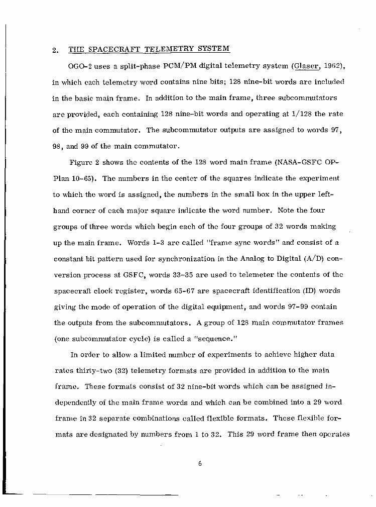
2. THE SPACECRAFT TELEMETRY SYSTEM
OGO-2 uses a split-phase PCM/PM digital telemetry system (Glaser, 1962),
in which each telemetry word contains nine bits: 128 nine-bit words a re included
in the basic main frame. In addition to the main frame, three subcommutators
a re provided, each containing 128 nine-bit words and operating at 1/128 the rate
of the main commutator. The subcommutator outputs are assigned to words 97,
98, and 99 of the main commutator.
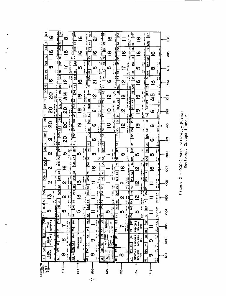
Figure 2 shows the contents of the 128 word main frame (NASA-GSFC OP-
Plan 10-65). The numbers in the center of the squares indicate the experiment
to which the word is assigned, the numbers in the small box in the upper Ieft-
hand corner of each major square indicate the word number. Note the four
groups of three words which begin each of the four groups of 32 words making
up the main frame. Words 1-3 are called “frame sync words’’ and consist of a
constant bit pattern used for synchronization in the Analog to Digital (A/D) con-
version process at GSFC, words 33-35 are used to telemeter the contents of the
spacecraft clock register, words 65-67 are spacecraft identification (ID) words
giving the mode of operation of the digital equipment, and words 97-99 contain
the outputs from the subcommutators. A group of 128 main commutator frames
(one subcommutator cycle) is called a “sequence.”
In order to allow a limited number of experiments to achieve higher data
rates thirty-two (32) telemetry formats are provided in addition to the main
frame. These formats consist of 32 nine-bit words which can be assigned in-
dependently of the main frame words and which can be combined into a 29 word
frame in 32 separate combinations called flexible formats. These flexible for-
mats are designated by numbers from 1 to 32. This 29 word frame then operates
6
I
hl
-7-
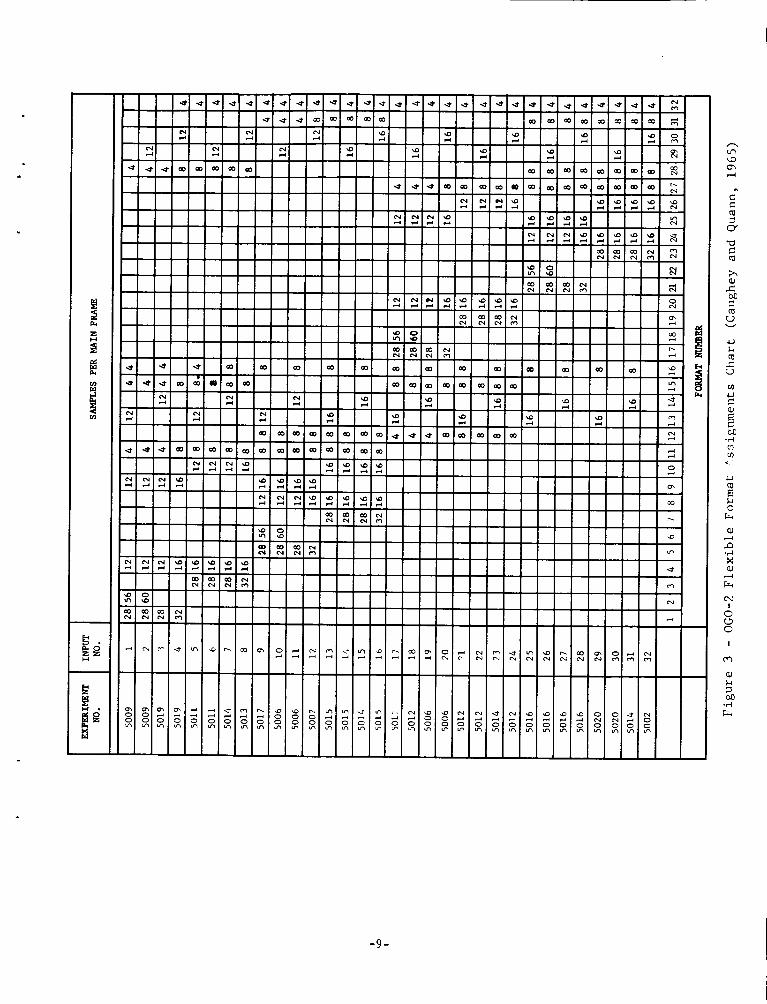
at the same bit rate as the main frame with the 29 flexible-format words re-
placing the last 29 words in each of the four 32 word groups in the main frame.
For example, Table 1 shows the word sampling sequence for flexible format 12,
one of those most frequently used
Table 1
Word Configuration of Flexible Format 12
X X X 20 21 22 23 24
9 10 11 12 13 14 15 16
17 18 19 20 21 22 23 24
9 10 11 12 13 14 15 16
The 32 words shown replace 32 words in the main frame, except the groups of
three discussed previously. Flexible format word 10 appears twice in the 32
word format and will therefore recur eight times in the main frame when o p
erating in FF12 mode. Figure 3 shows the sampling rate in the main frame
from the various experiments when operating in the various flexible format
modes.
Basic formatting and timing is handled in the digital data handling assembly
(ddha) (Glaser -3 1962) which contains two redundant groups of digital equipment.
Two tape recorders are carried, each with a capacity of 43.2 million bits, and
the two equipment groups a re designed such that while output is being recorded
on an on-board tape recorder, the other output may be fed to the transmitter for
real time operation to a ground station. The tape recorder operates at a main
8
-9 -
frame rate of 4000 bits/sec (4 kbs) and can record for three hours; the two re-
corders have a total storage capability of six hours. The recorders read out to
ground at 128 kbs enabling them to play back to ground in about 1 2 minutes when
both are filled to capacity. The ddha can also operate at 64 kbs and 16 kbs, upon
ground command, when in the real time mode.
The ddha provides accurate timing pulses (stability better than one part in
l o 5 , Farthing and Folz, 1966 and Ludwig, 1963) to the experiments at rates of
10 pps and 1 pps. The 1 pps signal is counted within the ddha and the (cumula-
tive) count is stored in the spacecraft clock register. This clock register is
interrogated by the telemetry system once each main frame.
3. MAGNETOMETER AND ASSOCIATED INSTRUMENTATION
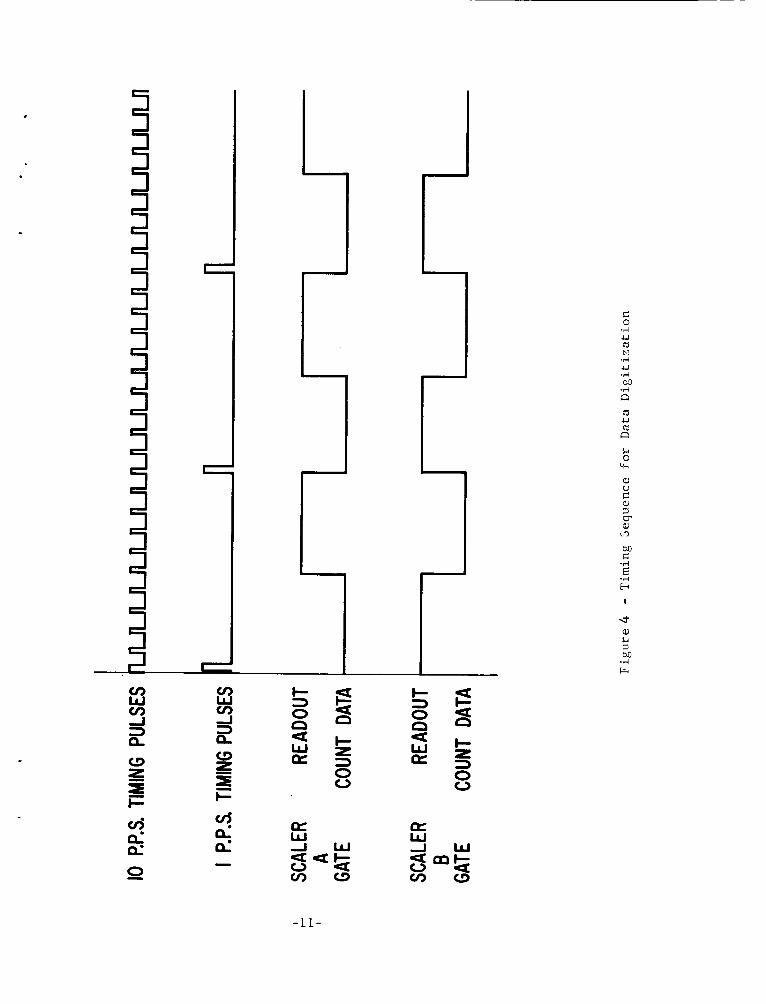
The magnetic field data originates with the output of an optically pumped,
self-oscillating, rubidium vapor magnetometer (Farthing and Folz, 1966) (using
Rb85). The resulting frequency (in cps) is equal to 4.66737 times the scalar
magnitude of the ambient magnetic field (in gammas). This frequency is sam-
pled on alternate half seconds by two electronic scalers, designated Scaler A
and Scaler B. The sequence of events is as follows (see Figure 4):
a) One second timing pulse from spacecraft occurs.
b) Scaler A samples data for approximately 1/2 second (determined by
counting the 10 pps signal).
While Scaler A is sampling data, Scaler B is available for readout to
both equipment groups. The information readout will be the count
c)
accumulated during the previous half second.
The output from each scaler consists of an accumulated count of up to 18
bits. Scaler A output appears in main frame words 57 and 58 and flexible
10
L. e E
e e
G e E
c e L
e e e c e E
e E e e L-
e E
e c E
E r v) W v) -I 3 e W z I F:
I
c 0
m U E P
a, u C
-11-
format words 10 and 11; Scaler B output appears in main frame words 121 and
122 and in flexible format words 19 and 20. Since the spacecraft operates at
4 KBS, 16 KBS, o r 64 KBS and the main frame consists of 1152 bits (128 nine-
bit words), the main frame will be read out in .288, .072, and .018 seconds
respectively and the spacecraft sequence durations (see Section 2 for definition
of a spacecraft sequence) will be 36.864, 9.216, and 2.304 seconds. Because of
the rate difference between the half second sampling times and the times between
readouts, the same data point may be read out in more than one frame. At
4 KBS it is possible to have either one or two complete readouts (or one com-
plete and one partial). At 16 and 64 KB main frame, and for flexible formats
at all bit rates, more than six readouts will occur for each data point. When
the experiment is interrogated during the half second allocated to counting the
value readout will be zero.
In addition to the digitized field data, various engineering data is telemetered
to ground from the experiment. These include the amplitude of the magnetometer
signal, temperatures at critical points in the instrument, power and heater
status and the band selection of an electronic comb filter used to increase the
signal to noise ratio of the magnetometer signal before scaling. These occupy
main frame words 59 and 123, and words 6, 50, 51, 52, 70, 114, 115, and 116 of
one of the subcommutators.
4. DATA REDUCTION BEFORE DATA REACHES THE EXPERIMENTER"
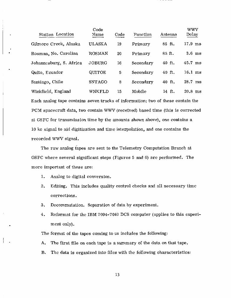
Data from the spacecraft is recorded on analog tape at two primary and
four secondary ground stations:
*Caughey and Quann, August 1965.
1 2
I -
I .’
Code wwv Station Location Name Code Function Antenna Delay -
Gilmore Creek, Alaska ULASKA 19 Primary 85 ft . 17.9 m s
Rosman, No. Carolina ROSMAN 20 Primary 85 f t . 3.6 m s
Johannesburg, S. Africa JOBURG 16 Secondary 40 ft . 45.7 m s
Quito, Ecuador QUITOE 5 Secondary 40 ft . 16.1 ms
Santiago, Chile SNTAGO 8 Secondary 40 ft. 28.7 ms
Winkfield, England WNKFLD 15 Mobile 14 ft. 20.8 m s
Each analog tape contains seven tracks of information: two of these contain the
PCM spacecraft data, two contain WWV (received) based time (this is corrected
at GSFC for transmission time by the amounts shown above), one contains a
10 kc signal to aid digitization and time interpolation, and one contains the
recorded WWV signal.
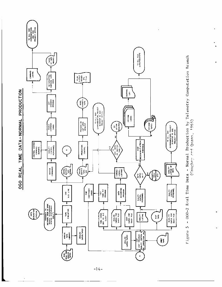
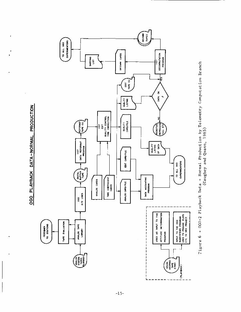
The raw analog tapes are sent to the Telemetry Computation Branch at
GSFC where several significant steps (Figures 5 and 6) a re performed. The
more important of these are:
1. Analog to digital conversion.
2. Editing. This includes quality control checks and all necessary time
corrections.
3. Decommutation. Separation of data by experiment.
4. Reformat for the IBM 7094-7040 DCS computer (applies to this experi-
ment only).
The format of the tapes coming to us includes the following:
A. The first file on each tape is a summary of the data on that tape.
B. The data is organized into files with the following characteristics:
13
sg 0 c x :Y
I \ I
.
I I d
!d
C 0
m
h Ll
.rl n
U m P
-15-
1.
2.
Data within a file is all from the same (Greenwich) day.
Data within a file is all of the same format (as regards bit rate,
etc.).
Data within a file is all from a particular ground station. 3.
Each file begins with a label record describing that file (including the date).
C, Each data record contains the data from one spacecraft sequence
including:
1.
2.
The time of the first bit of the sequence.
The time of some high resolution point (to be defined later) occur-
ring within that sequence ( i f determinable).
The clock readouts from the spacecraft. 3.
4. The experiment data itself.
This means that one record contains 35.864 sec. of data at 4 KBS, 9.216 sec.
at 16 KBS, and 2.304 sec. at 64 KBS.
5 . OUTLINE OF EXPERIMENTER DATA REDUCTION PROCEDURES
Up to this point we have described only steps through which the data passes
before coming to the experimenter. The data is essentially still "raw." This
raw data is then run through a series of computer programs (on an IBM 7094-
7040 direct couple system) to:
1) Weed out suspect data
2) Provide a tape of good data suitable for analysis.
A detailed description of the procedures will follow in subsequent sections. A
brief description is as follows:
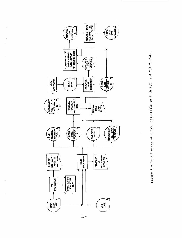
A. The bulk of the processing, including the weeding out of the suspect data
is done in the "MAIN PROCESSOR." (See Figure 7) The data is divided
16
4 %
t
-2 W W
I I
m
P
U m
.o C m
? d s 3 !n 0 U
Q) 4 P m U .r( 4 n. a c
Y
- 1 7 -
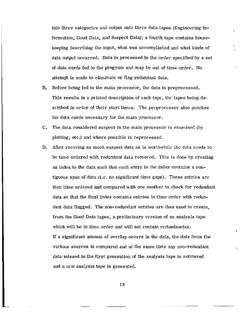
into three categories and output onto three data tapes (Engineering In-
formation, Good Data, and Suspect Data); a fourth tape contains house-
keeping describing the input, what was accomplished and what kinds of
data output occurred. Data is processed in the order specified by a set
of data cards fed to the program and may be out of time order. No
attempt is made to eliminate or flag redundant data.
Before being fed to the main processor, the data is preprocessed.
This results in a printed description of each tape, the tapes being de-
scribed in order of their start times. The preprocessor also punches
the data cards necessary for the main processor.
The data considered suspect in the main processor is examined (by
plotting, etc.) and where possible is reprocessed.
Af ter recoving as much suspect data as is worthwhile the data needs to
be time ordered with redundant data removed. This is done by creating
an index to the data such that each entry in the index contains a con-
tiguous span of data (i.e. no significant time gaps). These entries are
then time ordered and compared with one another to check for redundant
data so that the final index contains entries in time order with redun-
dant data flagged. The non-redundant entries a re then used to create,
from the Good Data tapes, a preliminary version of an analysis tape
which will be in time order and will not contain redundancies.
If a significant amount of overlap occurs in the data, the data from the
various sources is compared and at the same time any non-redundant
data missed in the first generation of the analysis tape is retrieved
and a new analysis tape is generated.
B.
C.
D.
18
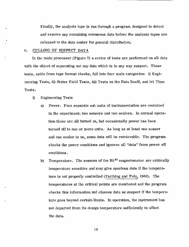
Finally, the analysis tape is run through a program designed to detect
and remove any remaining erroneous data before the analysis tapes a re
released to the data center for general distribution.
6. CULLING OF SUSPECT DATA
In the main processor (Figure 7) a series of tests a re performed on all data
with the object of separating out any data which is in any way suspect. These
tests, aside from tape format checks, fall into four main categories: i) Engi-
neering Tests, ii) Status Field Tests, iii) Tests on the Data Itself, and iv) Time
Tests.
i) Engineering Tests
a) Power. Four separate sub units of instrumentation a re contained
in the experiment; two sensors and two scalers. In normal opera-
tion these a re all turned on, but occasionally power has been
turned off to one o r more units. As long as at least one sensor
and one scaler is on, some data will be retrievable. The program
checks the power conditions and ignores all 7'data" from power off
conditions.
Temperature. The sensors of the Rbg5 magnetometer are critically b)
temperature sensitive and may give spurious data if the tempera-
ture is not properly controlled (Farthing and Folz, 1966). The
temperatures at the critical points are monitored and the program
checks this information and classes data as suspect if the tempera-
ture goes beyond certain limits. In operation, the instrument has
not departed from its design temperature sufficiently to affect
the data.
19
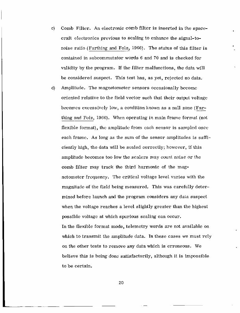
c) Comb Filter. An electronic comb filter is inserted in the space-
craft electronics previous to scaling to enhance the signal-to-
noise ratio (Farthing and Folz, 1966). The status of this filter is
contained in subcommutator words 6 and 70 and is checked for
validity by the program. If the filter malfunctions, the data will
be considered suspect. This test has, as yet, rejected no data.
d) Amplitude. The magnetometer sensors occasionally become
oriented relative to the field vector such that their output voltage
becomes excessively low, a condition known as a null zone (Far-
thing and Folz, 1966). When operating in main frame format (not
flexible format), the amplitude from each sensor is sampled once
-
each frame. As long as the sum of the sensor amplitudes is suffi-
ciently high, the data will be scaled correctly; however, if this
amplitude becomes too low the scalers may count noise o r the
comb filter may track the third harmonic of the mag-
netometer frequency. The critical voltage level varies with the
magnitude of the field being measured. This was carefully deter-
mined before launch and the program considers any data suspect
when the voltage reaches a level slightly greater than the highest
possible voltage at which spurious scaling can occur.
In the flexible format mode, telemetry words a re not available on
which to transmit the amplitude data. In these cases we must rely
on the other tests to remove any data which is erroneous. We
believe this is being done satisfactorily, although it is impossible
to be certain.
20
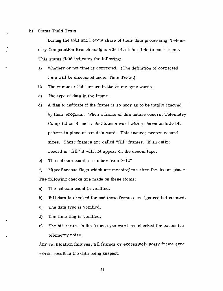
ii) Status Field Tests
During the Edit and Decom phase of their data processing, Telem-
etry Computation Branch assigns a 36 bit status field to each frame.
This status field indicates the following:
a) Whether or not time is corrected. (The definition of corrected
time will be discussed under Time Tests.)
The number of bit e r rors in the frame sync words.
The type of data in the frame.
A flag to indicate if the frame is so poor as to be totally ignored
by their program. When a frame of this nature occurs, Telemetry
Computation Branch substitutes a word with a characteristic bit
pattern in place of our data word. This insures proper record
sizes. These frames a re called 77fill '7 frames. If an entire
record is 77fil177 it will not appear on the decom tape.
The subcom count, a number from 0-127
Miscellaneous flags which are meaningless after the decom phase.
b)
c)
d)
e)
f)
The following checks are made on these items:
a)
b)
c)
d)
e)
The subcom count is verified.
Fill data is checked for and these frames are ignored but counted.
The data type is verified.
The time flag is verified.
The bit errors in the frame sync word are checked for excessive
telemetry noise.
Any verification failures, f i l l frames or excessively noisy frame sync
words result in the data being suspect.
2 1
iii) Data Tests
These tests are applied to the data themselves and, considered as
a whole, have proven very successful in weeding out bad data.
a) Redundant readouts. It has been previously mentioned that fre-
quently the data counted during one half second may be read out in
telemetry frames more than once during the next half second. The
program knows the time relationships between the timing pulses
and the readout times and can predict when multiple readouts will
occur and how many to expect (from 2 to 25 depending upon format).
If a certain number (always greater than 80%) of these a re not equal
the data point is considered suspect.
b) Reference check. Since the theoretical descriptions of the earth's
field in the range of altitudes traversed by POGO is already known
to within a few percent, a good method of detecting severe e r ro r is
to compare measured and theoretic field. The theoretic field cur-
rently used is the GSFC(4/64) field (Cain, et al., October 1964). If
the measured field differs by more than 500 gammas for this theo-
retic field, the data point is considered suspect.
In order to minimize the computation necessary in this check, an
approximation to the theoretic field is used. This is determined by
choosing three field points spaced no more than 37 seconds (of
time) apart on the orbital path of the satellite. A parabola passing
through the three points is computed and, for times lying within
the two end times, the result is used for the theoretical field.
22
Extensive tests were made which indicate this approximation *
to be within one gamma of the original theoretic field.
All previously discussed tests result in individual data points being
considered suspect. It is felt, however, that when the amount of data
points considered suspect reaches a certain percentage of the total
data input that it would be wise to reject entire records of data (A
record, you will recall, is one spacecraft sequence, 36.864 seconds of
4 KB data.) and this procedure is followed for both of the above de-
scribed tests. Some checks apply only to entire records being rejected;
these include the next two to be discussed.
c)
-
Zero check. When the ddha interrogates a scaler during the half
second when the scaler is counting, the readout will be zero. If
these readouts are non-zero when we receive the data, then the
spurious value has been substituted for the original zero sometime
between the interrogation by the ddha and the output by the decom
program of the Telemetry Computation Branch. Presumably these
non-zero values result during the A/D conversion whenever the S/N
ratio is poor. For 4 KBS main frame data, a count is kept of the
number of these readouts which a re non-zero. This is believed to
be a measure of the quality of the telemetry process. If the count
exceeds a certain limit (currently set at six for each scaler, i.e. if
the count for one scaler reaches six), the entire record is consid-
ered suspect.
Differencing check. The difference test is a limit test of the second
differences of the data. Whenever three successive data points a r e
d)
23
available (i.e. not rejected by a previous check) the second differ-
ence is computed, and if it is too large a counter is advanced. The
current limit used for the second difference is 20 gammas. If the
counter becomes too large the entire record is considered suspect.
The current limits on the counter are 15 at 4 KB, 5 at 16 KB, and
3 at 64 KB. Due to the fact that this test does not reject individual
data points it has proved useful only under circumstances where
the data has a significant amount of scatter but is not erroneous
enough to fail the reference check.
iv) Time Tests
It is extremely important that the correct time be associated with
each data point, OGO-2 may encounter field gradients of up to 40y/sec
(see Section 11, Data Quality) which gives a possibility of an equivalent
error of ly if the time is incorrect by 25 msec.
There are essentially two different timing rates associated with
the spacecraft: 1) the timing pulses, from which the counting periods
fo r the scaling of the magnetic field data are determined and 2) the data
readout times which determine the format of the data received by the
experimenter. (Both of these timing pulses are derived from the same
master oscillator,) In order to process the data, we must know the
relationship between these timing rates and, in order to assign correct
time to the data, we must have an accurate estimate of the Universal
Time of each timing pulse. The main difficulty in accurately deter-
mining time stems from the fact that the telemetry contains no direct
indication of when the timing pulses are occurring.
24
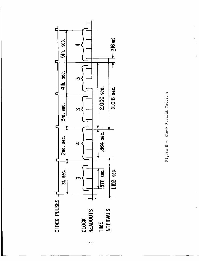
If the data format is carefully examined, it i s soon apparent that
the relationship of the two timing systems forms a predictable pattern.
For example, at 4 KBS it takes .288 sec. to read out one frame, i.e.
the clock register i s interrogated every .288 seconds. If we examine
Figure 8 we see clearly the type of pattern which emerges. In the
first , third, and fourth seconds three readouts occur (in .576 seconds)
and in the second and fifth seconds four readouts occur (in ,864 seconds)
The normal pattern is an alternating 3-4; three identical readouts, then
four, then three, then four, etc. This is occasionally interrupted by
two successive threes, as seen in the third and fourth seconds of
Figure 8. When this occurs the clock readout immediately preceding
(or following) the 3-3 combination i s called a high resolution point
(H.R.P.) because the 1st readout after o r before the 3-3 is within 16
milliseconds of a clock update. At 4 KBS this 3-3 occurs twice each
125 frames and then the entire pattern repeats. If both 3-3 combina-
tions are found, the relationship between the two time systems can be
determined to
seconds apart whereas the associated timing pulses will be 19.000
seconds apart. Similar patterns occur at 16 and 64 KBS which allow
resolution of the two time systems to at least It4 MS. The relationship
between the two time systems is always determined by finding high
resolution points, resulting in a possible e r ro r of *4 MS.
MS because the two 3-3 combinations occur 19.008
Turning our attention to real-time data only, recall that, as the
data from the spacecraft is recorded on analog tape at the ground
station, various time signals a re also recorded. These time signals
25
I
a re decoded in the STARS-1 time decoder (Demmerle, et al., 1964) as
' part of the A/D conversion, assigning U.T. to each frame as it is
digitized. These Universal Times are subsequently corrected (Caughey
and Quann, August 1965) for transmission time delays from 1) WWV to
the ground station, and 2) satellite to ground station. At this juncture
what is known as "time fitting" (Caughey and Quann, August 1965)
occurs. For a particular time interval a series of high resolution
points a re determined from a selected sample of edited real time data.
This results in a series of clock counts and associated universal times
which a re fed as data to a program which uses the least squares tech-
nique to determine a linear relationship between clock count and uni-
versal time. Maximum residuals to these fits are usually less than
20 milliseconds, often considerably less; typical root-mean-square
residuals are on the order of 3-9 milliseconds. The residuals are due
to a combination of several factors: the most obvious are: 1) short
term drift of the spacecraft clock, and 2) inaccuracies (and variability)
of the transmission time from WWV to the ground station. No further
fitting has been attempted, the results of the time fit being "fed back"
into the edit program so that all times on the data received by the
experimenter are derived from the f i t .
Playback data entails a different procedure since the U.T. on the
analog tape is meaningless. Time is assigned to the playback data by
finding a high resolution point and then determining the U.T. from the
fit derived from real time data during the same time period.
2 7
All of the above time correction is performed by the Telemetry
Computation Branch of GSFC before their Decom run, and only the re-
sults a re seen by the experimenter. When we receive the data the time
should be fully corrected in that all transmission times have been ac-
counted for and the relationship between readout time and the data
counting gates should be established to *4 ms. As a cross check, how-
ever, we enter as parameters into the main processor l) the slope of
the applicable time fit and 2) the time of some clock count during the
day --- for each day. These parameters a re sufficient so that given a U.T.
we can easily determine if it lies on the curve computed in the applica-
ble fit. At the start of each data file the program searches for a high
resolution point (H.R.P.) and, if one is found, compares it to the correct
fit. If it differs by more than 26 milliseconds the entire file is con-
sidered suspect. If the data is so bad that we a re unable to determine
a H.R.P. but we are furnished with one on the tape, the one furnished
is compared with the fit, using the same (or more stringent) cri teria
for passing the test. If a H.R.P. is found and we a re furnished with
one on the tape, both a re compared to the f i t . The 26 milli-
seconds was arrived at empirically.
12 milliseconds since their e r r o r is supposed to be -+4 milliseconds
and our H.R.P. determination is accurate to -+8 milliseconds. When
comparing their input H.R.P. to the time f i t the limit should ideally be
4 milliseconds. In practice, for C.S.P. data, the H.R.P. furnished on
the source data tapes a r e rarely over 1 ms. from the time f i t and our
computed H.R.P. are usually within the 12 ms. although a few cases of
differences up to 20 ms. have been found. For real time data the high
Ideally this limit should be
28
resolution points usually fal l between 1 and 20 ms. from the time fit.
We have recently discovered that the 16 KB time checks are usually
within 8 ms. while the 64 KB time checks a re usually between 12 ms.
and 22 ms. We conclude that the 64 KB times a re in error by the time
necessary to read out one frame, i.e. 18 ms. The source of this e r ror
is not yet known except that it is present on the tapes which we receive
from Telemetry Computation Branch.
A time test is also performed for each record within the file before
it is processed except that if a H.R.P. is furnished on the tape no search
is made for one in the data.
Another type of time check is made at the start of each record.
One of the input times in our data is the time of the first bit of the
sequence making up the current data record. Since each data record
covers a fixed period of time, the input time can be compared to a
previous input time. The difference between those times is required
to be equal to the time required for an integral number of records to
occur. The accuracy required in this test is ten milliseconds.
These tests have proved very successful. For example, several
programming errors were discovered in the Edit program of the
Telemetry Computation Branch which resulted in a high (about 25%)
percentage of real time files with bad time. These were rejected im-
mediately by the program. Inaccurate time has not been a major
problem with playback data except in a few instances. In the early
phases of data reduction we were receiving data which contained a time
error which slowly accumulated within a file at a rate of about ten
29
milliseconds per hour of data. This e r ror was detected on those files
whose time span exceeded 1.5 hours, the nature of the e r ro r was deter-
mined, and our programs fixed to eliminate the error.
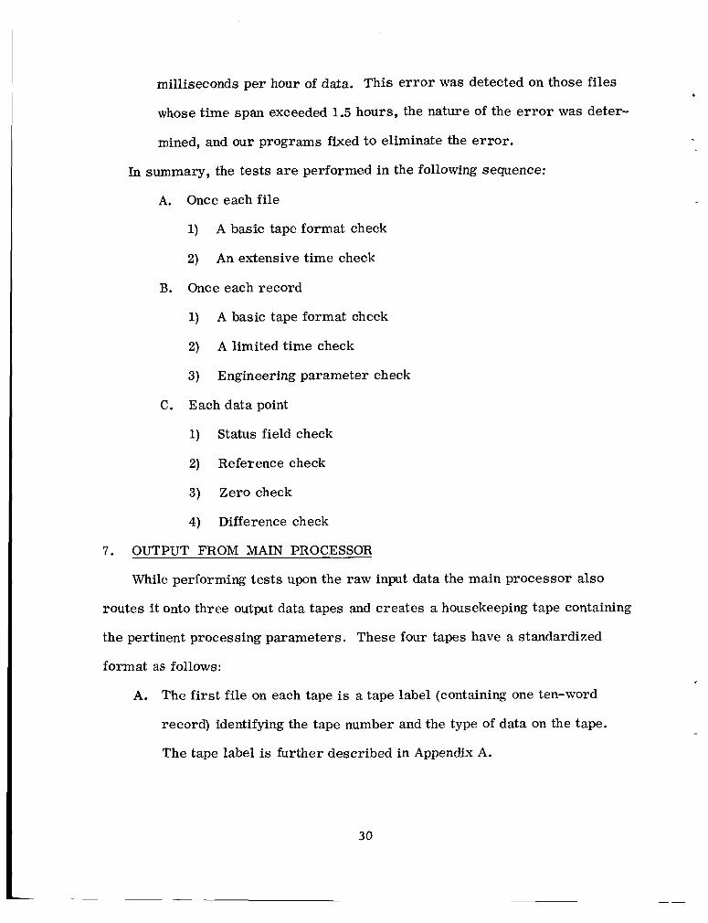
In summary, the tests a re performed in the following sequence:
A. Once each file
1)
2) An extensive time check
A basic tape format check
B. Once each record
1)
2) A limited time check
3) Engineering parameter check
A basic tape format check
C. Each data point
1) Status field check
2) Reference check
3) Zero check
4) Difference check
7. OUTPUT FROM MAIN PROCESSOR
While performing tests upon the raw input data the main processor also
routes it onto three output data tapes and creates a housekeeping tape containing
the pertinent processing parameters. These four tapes have a standardized
format as follows:
A. The first file on each tape is a tape label (containing one ten-word
record) identifying the tape number and the type of data on the tape.
The tape label is further described in Appendix A.
.
30
B. Each successive file is a data file. The first record on each data file,
for all four tape types, is a (15 word) record, called a File Housekeep-
ing, describing the file.
C. All records following the File Housekeeping are data records. These
a re peculiar to the type of tape involved.
Each input file is processed as an entity and, if it results in output of a
particular type, all of that output will be contained in the same file on each
output tape. Thus each input file results in one File Housekeeping record
which is always output onto the Housekeeping tape. If the entire file is suspect
(e.g. erroneous time o r erroneous tape format) the only other output will be to
the tape containing suspect data (called the Garbage tape). If, on the other hand,
some good data results, the File Housekeeping will also be written on the tape
containing engineering information (called the Subcom- Amplitude tape, o r
SATAPE), and the tape containing good data (called the Good Data tape). Since
the File Housekeeping applies to only one input file, all information describing
that input file is placed in the file housekeeping including the date and data type.
For a complete description of the contents of the File Housekeeping see
Appendix A.
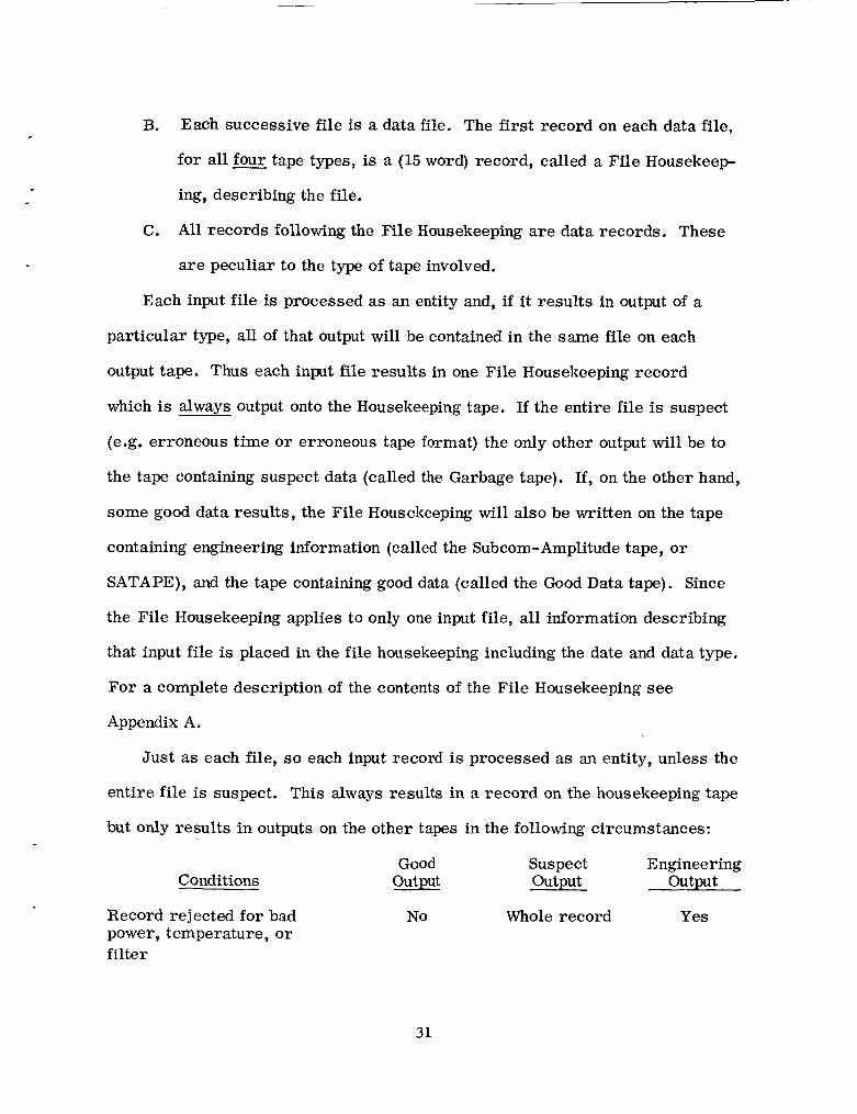
Just as each file, so each input record is processed as an entity, unless the
entire file is suspect. This always results in a record on the housekeeping tape
but only results in outputs on the other tapes in the following circumstances:
Good Suspect Engineering Conditions output Output Output
Record rejected for bad power, temperature, or filter
No Whole record Yes
31
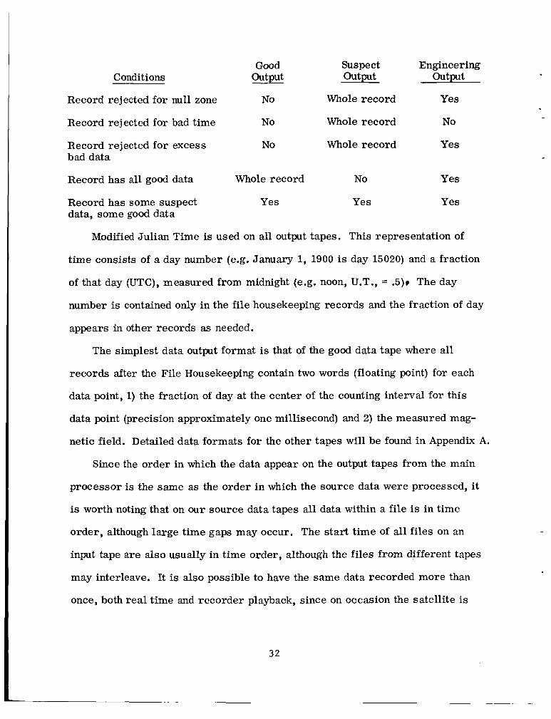
Conditions
Record rejected for null zone
Record rejected for bad time
Record rejected for excess bad data
Record has all good data
Record has some suspect data, some good data
Good Suspect Engineering Output output Output
No Whole record Yes
No Whole record No
No Whole record Yes
Whole record No Yes
Yes Yes Yes
Modified Julian Time is used on all output tapes. This representation of
time consists of a day number (e.g. January 1, 1900 is day 15020) and a fraction
of that day (UTC), measured from midnight (e.g. noon, U.T., = .5)r The day
number is contained only in the file housekeeping records and the fraction of day
appears in other records as needed.
The simplest data output format is that of the good data tape where all
records after the File Housekeeping contain two words (floating point) for each
data point, 1) the fraction of day at the center of the counting interval for this
data point (precision approximately one millisecond) and 2) the measured mag-
netic field. Detailed data formats for the other tapes will be found in Appendix A.
Since the order in which the data appear on the output tapes from the main
processor is the same as the order in which the source data were processed, it
is worth noting that on our source data tapes all data within a file is in time
order, although large time gaps may occur, The start time of all files on an
input tape are also usually in time order, although the files from different tapes
may interleave. It is also possible to have the same data recorded more than
once, both real time and recorder playback, since on occasion the satellite is
32
visible to two (and, rarely three) ground stations simultaneously. This results
in output tapes which a re not completely in time order and which contain re-
dundant data.
8. RECOVERY OF SUSPECT DATA
The checks performed on the data in the main processor may consider data
suspect, and consequently reject it, on one of three levels. If only a few data
points in a record are suspect they may be output to the suspect data tape as
individual points without rejecting the entire source record. If, however, some
data check is failed by too many points o r the record fails an engineering or
time test, the entire record will be output to the suspect data tape. The worst
case is when an entire file is of such anature as to be unprocessable and is
consequently rejected in its entirety. When designing the Main Processor (see
Section 13) it was decided not to mix good and suspect data on the same output
tape. At that time little was known of the types of suspect data which would
arise in practice or of what recovery techniques might be possible. As of this
writing a recovery program has been written and successfully applied to the
command storage playback data from the period 10/14/65 to 10/24/65. The
program was then revised in the light of our experience with the October data
and applied to the data from 10/29/65 to 11/15/65. It is these results which are
reported here.
In considering the recovery problem, the real time data is in a different
class from the playback data because the number of real time data points is
less than 1/5 that obtained from playback data. Since the effort necessary for
the recovery of real time data is about twenty times more per data point than
for playback (due to the multiplicity of readouts for each data point resulting
33
from the higher bit rates), making a recovery effort very costly for the small
amount of data which might be retrieved, we decided to make no effort to re-
cover suspect real time data.
Two criteria determined whether or not we attempted to recover suspect
playback data:
of the data, and 2) is there a reasonable chance of recovering a significant
amount of the chunk.
1) is it in a chunk large enough to be significant for the analysis
A s discussed in Section 6 , suspect data falls into four broad categories:
1. Format or tape read errors rendering the data unprocessable
2. Entire files rejected when the time differs from the time fit
3 . Entire records rejected because
a) power was turned off
b)
c) time is inaccurate
d)
Individual data points rejected becau
a null zone has occurred
the data itself fails a test
4. e the data it elf fails a test.
Approximately 1.2% of the total data set falls into category four. This data is
widely scattered throughout the total data set and no recovery was attempted.
We are unable to cope adequately with data in Category 1; this data is reproc-
essed by the Telemetry Computation Branch after which it goes back through
the main processor.
Some file level time rejections (Category 2) were found to be caused by the
input times being placed in the record preceding the correct record. These
were easily corrected and most of the data successfully recovered. Inaccurate
time on individual records caused only one large block of data to be rejected (as
34
of this writing). This large block was found to be due to a slowly accumulating
time e r ro r (see Section 6 , Time Tests) whose rate of accumulation was found,
the times corrected, and most of the data recovered.
It was found for records being rejected because too many data point failed
the reference or zero tests, that, in most cases, more individual data points
could be rejected before considering the entire record suspect. This procedure
does not unduly increase the number of bad points escaping detection, and it is
these types of suspect data which form the bulk of the data recovered.
The process of recovery proceeds as follows:
A.
B.
C.
D.
Data processing summaries are examined to find where chunks of re-
jected data over 5-10 minutes long have occurred.
If the underlying cause of rejection is not understood (as with most
suspect time) printouts of the original data records a re carefully
examined (by hand) to gain an understanding of the problem.
If there is any doubt as to the recoverability of the data or as to the
quality of the data being recovered, plots of both measured field and
A F (measured field minus theoretical field) a re made and examined
carefully.
Only after the reason for the data being suspect is thoroughly under-
stood and the recoverability is established does the actual recovery
take place. At this time the original housekeeping record (or file) is
flagged, indicating that the. data has been reprocessed, and a new house-
keeping file is added to the housekeeping tape summarizing the results
of the recovery attempt. The recovered good data is organized into
new data files and added to the end of the good data tape applicable to
the period of time into which the data falls.
35
Reprocessing consists of passing the data through the same tests as a re
in the main processor with the rejection levels reset so that most of the
data will no longer be rejected. In addition, the reprocessed data is
selectively plotted to be sure the resulting data is of acceptable quality.
For data from times subsequent to 10/24/65 an additional data check
has been added during reprocessing of suspect data. After all other
tests have been performed on a record (since this is always playback
data, one record is 36.864 seconds of data), an array of measured
minus theoretical field, called A F , (theoretic field computed as de-
scribed in Section 6, iii, b) is formed. A least-squares, linear, f i t is
made to the AF array and the average absolute deviation from the fit is
computed. Any points deviating by more than five times the resulting
average are then rejected. If the resulting average is above .4 gammas
the f i t is repeated, up to five times, unless two successive fits result in
the same average. If after all iterations have been completed the aver-
age is still above 2 gammas, none of the data is accepted.
9. A TIME ORDERED INDEX
When planning and coding the main processor we naively assumed that we
would receive the data in time order and with redundant records removed by the
Telemetry Computation Branch choosing the best of those that overlap. In
practice none of these criteria are completely met. The data is processed in
time order. insofar as is possible but there remain a significant number of over-
lapping and out-of-order files. In fact, some files have time gaps of 2-3 hours
where the data from the gap is contained in a different file. The housekeeping
tape was originally intended to serve not only as a summary of the data
36
processing procedure but also as a handy index, time ordered, to the data. It
was soon apparent that time-ordering the housekeeping tapes and flagging re-
dundant data during the data reduction process would entail a large programming
effort and use large amounts of computer time. At this juncture the concept of
an index tape was invented.
The generation of an index tape occurs in three steps. First, the house-
keeping tape is scanned and, as long as there are no time gaps over five minutes,
one entry is made in the index tape for each file. This includes the following
information:
1)
2)
3) The date
4)
5)
6)
7)
8)
Housekeeping tape and file number
Good data tape and file number
The start and stop fraction of day
The number of records on the housekeeping file
The number of records on the good file
The start and stop record numbers on the housekeeping tape
The start and stop record number on the good data tape
If a time gap (or gaps) of over five minutes occurs, more than one entry per
file will result; thus the data described by an entry will contain no time gaps of
over five minutes. The second step in the process is to order the index entries
by time.
In the third step, redundant data is flagged. This is done by considering
successive entries on the index; we know that the earlier entry begins before
(or at the same time as) the following one. If the times of some entry are com-
pletely contained within the times of a previous entry, the (later) entry is flagged
3 7
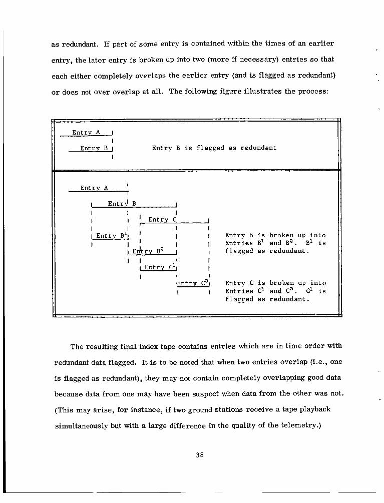
as redundant. If part of some entry is contained within the times of an earlier
entry, the later entry is broken up into two (more if necessary) entries so that
each either completely overlaps the earlier entry (and is flagged as redundant)
o r does not over overlap at all. The following figure illustrates the process:
1
Entry A I I
I Ent ry B I Ent ry B i s f l a g g e d a s redundant
1 1
E n t r y A
I E n t r d B 1 I I I I I I E n t r y C I I I . I I
1
I Ent ry B1[ ' I I Ent ry i s broken up i n t o I I . I I I E n t r i e s B1 and B a . B1 i s
I E r k r v B2 I f l a g g e d as r edundan t . I I I I I
I I I @ t r y Caj Ent ry C i s broken up i n t o I I E n t r i e s C1 and C2 . C1 i s
f l a g g e d a s r edundan t .
I Ent ry C1l I
The resulting final index tape contains entries which are in time order with
redundant data flagged. It is to be noted that when two entries overlap (i.e., one
is flagged as redundant), they may not contain completely overlapping good data
because data from one may have been suspect when data from the other was not.
(This may arise, for instance, if two ground stations receive a tape playback
simultaneously but with a large difference in the quality of the telemetry.)
38
10. DATA FOR ANALYSIS
The end product of any data reduction procedure must be a data set in a
form both suitable and convenient for analysis of that data. We have used the
following criteria for our final data tapes, called Analysis Tapes:
1.
2.
The data should be easily accessible to the FORTRAN programmer.
The data should be in time order, each data point appearing only once
on the tape (i.e., no redundant data).
Only good (non-suspect) data should appear on the tape. 3.
The resulting format is a binary tape generated by IBM 7094 FORTRAN
IOCS and therefore readable by same. It contains no tape label. All records
a re two hundred (200) words in length and each file contains all the (available,
good) data from a particular day. End-of-tape is indicated by two successive
tape marks. Within each file the first record is a label such that the f i rs t word
contains the modified Julian Day number of the data in that file and the second
word contains the day number (MJD) on which the file was generated from the
good data tapes. Both of these words are fixed point and the res t of the words
in the record a re unused.
Each data record contains 100 data points, each in two floating point words,
the first being the fraction of day of the data point and the second, the value of
the magnetic field in gammas. The time system is that described in Section 7.
The final version of the analysis tape is derived in several steps. (See
Figure 7) First, the non-redundant entries on the index tape a re used to retrieve
data from the good data tape in time order with no overlap. This results in a
preliminary version of the analysis tape. Next, the redundant entries on the
index tape a re used to retrieve the data from the good tape which should overlap
39
data already put on the preliminary analysis tape. During this process the re-
dundant data from the good tape is compared, both in time and in magnetic field
value, with its counterpart on the good tape. A summary of the comparison re-
sults is contained in the section on data quality. If any points a re found on the
good data tape which a re not already on the analysis tape they a re set aside in a
scratch tape and then merged with the data on the preliminary tape to form an
intermediate analysis tape.
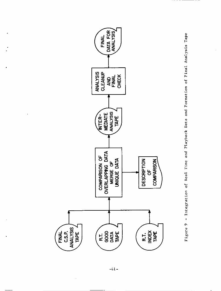
Formation of these analysis tapes utilizes only command storage playback
data. At this stage in the processing we have a C.S.P. analysis tape (the inter-
mediate analysis tape) and an R.T. index and good data tape. (See Figure 9) The
same type of data comparison is then done between the R.T. data and C.S.P. data
as was done between the overlapping C.S.P. data, resulting in a point by point
comparison of equivalent data points and a merging of unique data points into
another intermediate analysis tape.
The final step in the data reduction process is a general clean-up and double
checking of the analysis tape to be released to the data center. A final data test
is performed, called the O F f i t test, to attempt to eliminate any remaining
spurious data and the tape is checked to be sure that the data is indeed in time
order and has no redundant data.
The AF f i t test consists of fitting a linear curve to one record of analysis
data, unless a time gap of over 30 seconds occurs, in which case multiple fits
occur as long as a f i t interval contains six o r more points. In order to achieve
a more sensitive test, the fit is not made to the data itself but rather to the value
of A F (difference between the measured field and a theoretical field) computed
using the GSFC (9/65) coefficients. The rms of the residuals to the fit is then
40
t
a
t
(D C c
w 0
C 0 -rl U m E &I 0 Fr 'F) C m m u m
2 W m P h m d P+
'F) C m
ca
aJ E
w 0
-41 -
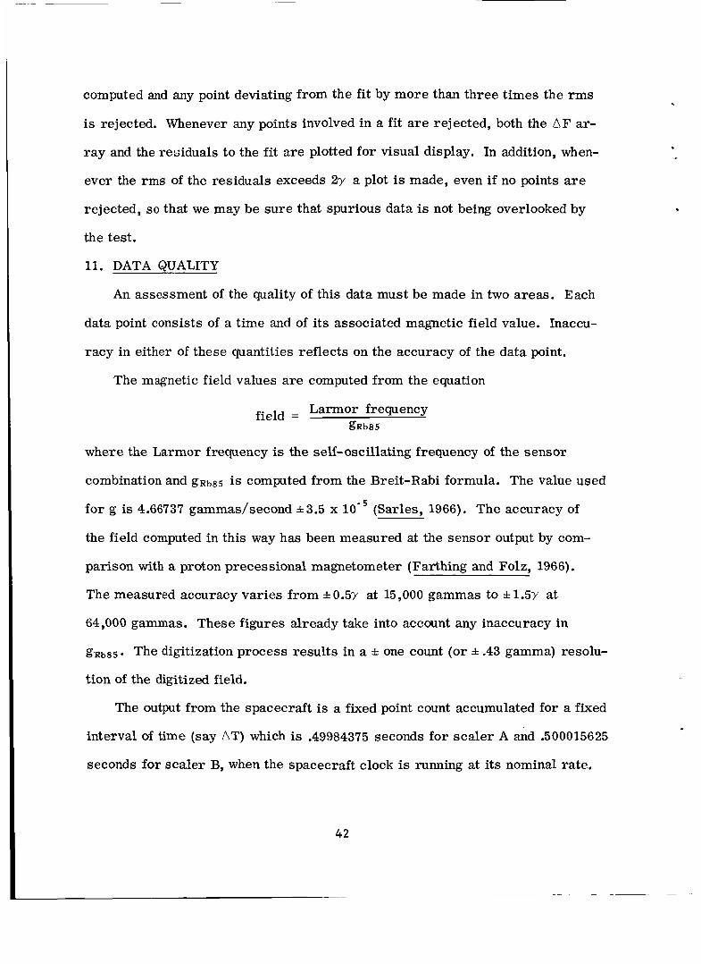
computed and any point deviating from the fit by more than three times the rms
is rejected, Whenever any points involved in a fit a re rejected, both the A F ar-
ray and the residuals to the fit are plotted for visual display. In addition, when-
ever the rms of the residuals exceeds 27 a plot is made, even if no points are
rejected, s o that we may be sure that spurious data is not being overlooked by
the test.
11. DATA QUALITY
An assessment of the quality of this data must be made in two areas. Each
data point consists of a time and of its associated magnetic field value. Inaccu-
racy in either of these quantities reflects on the accuracy of the data point.
The magnetic field values are computed from the equation
Larmor frequency field = gRb85
where the Larmor frequency is the self-oscillating frequency of the sensor
combination and gRb85 is computed from the Breit-Rabi formula. The value used
for g is 4.66737 gammas/second *3.5 x lo-’ (Sarles, 1966). The accuracy of
the field computed in this way has been measured at the sensor output by com-
parison with a proton precessional magnetometer (Farthing and Folz, 1966).
The measured accuracy varies from f 0.5” at 15,000 gammas to f 1.5” at
64,000 gammas. These figures already take into account any inaccuracy in
gRb8s. The digitization process results in a f one count (or f .43 gamma) resolu-
tion of the digitized field.
The output from the spacecraft is a fixed point count accumulated for a fixed
interval of time (say AT) which is .49984375 seconds for scaler A and .500015625
seconds for scaler B, when the spacecraft clock is running at its nominal rate.
42
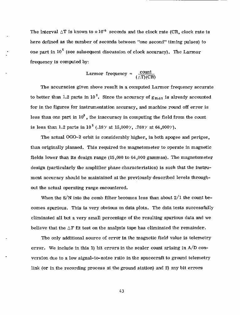
The interval AT is known to *1C6 seconds and the clock rate (CR, clock rate is
here defined as the number of seconds between "one second" timing pulses) to
one part in l o 5 (see subsequent discussion of clock accuracy). The Larmor
frequency is computed by:
The accuracies given above result in a computed Larmor frequency accurate
to better than 1.2 parts in 10'. Since the accuracy of g R b 8 5 is already accounted
for in the figures for instrumentation accuracy, and machine round off error is
less than one part in lo8 , the inaccuracy in computing the field from the count
is less than 1.2 parts in l o 5 (.18Y at 15,00OY, .768Y at 64,OOOY).
The actual OGO-2 orbit is considerably higher, in both apogee and perigee,
than originally planned. This required the magnetometer to operate in magnetic
fields lower than its design range (15,000 to 64,000 gammas). The magnetometer
design (particularly the amplifier phase characteristics) is such that the instru-
ment accuracy should be maintained at the previously described levels through-
out the actual operating range encountered.
When the S/N into the comb filter becomes less than about 2/1 the count be-
comes spurious. This is very obvious on data plots. The data tests successfully
eliminated all but a very small percentage of the resulting spurious data and we
believe that the A F f i t test on the analysis tape has eliminated the remainder.
The only additional source of error in the magnetic field value is telemetry
error. We include in this 1) bit errors in the scaler count arising in A/D con-
version due to a low signal-to-noise ratio in the spacecraft to ground telemetry
link (or in the recording process at the ground station) and 2) any bit errors
43
introduced in our data when being edited and decommed by the Telemetry Com-
putation Branch at GSFC (see Section 4). No evidence of the latter has been
found.
Bit errors can be difficult to detect since an e r ror in the least significant
bit is equivalent to an error of only .42 gammas. We believe that our data
checks are eliminating the vast majority of data containing this type error. All
of the data points at 16 KB and 64 KB have duplicate readouts and over 50% of
the data points at 4 KB have duplicate readouts. It is unlikely that telemetry
noise would effect these duplicate readouts in the same way which means that
the redundant readout test (Section 6, iii, a) should eliminate this problem for
over one-half of the data. For the rest of the data the reference, difference,
and zero checks will eliminate the worst cases and the A F fit test on the analysis
tape should catch the rest.
The best indicators of the quality of the telemetry signal are the amounts of
data rejected by the main processor when it is performing the various data
checks, and the percent of f i l l and noise frames which occur. Table 2 (the
Quality Summary) contains a summary of these indicators for the period 10/14
thru lo/%, 1965. Twelve percent of the C.S.P. data from this period of time
was rejected in the main processor. (This figure does not include a few files
not processed when a preceding file on the source tape had a sufficient number
of tape redundancies to cause processing to cease altogether on that tape.) Over
one-quarter of the data rejected is accounted for by tape redundancies and another
quarter of the rejected data is accounted for by inaccurate time. However, 471
of the 526 records rejected by the time tests were later reprocessed and 466 of
them recovered. The quality summary shows how many records were
44
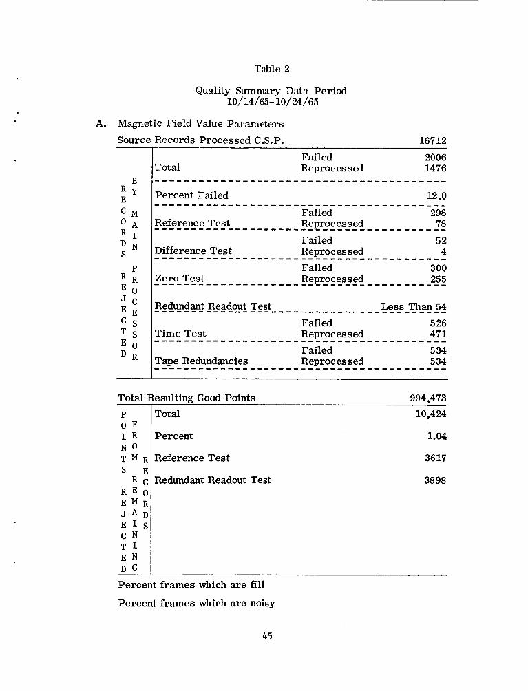
Table 2
Quality Summary Data Period 10/14/65- 10/24/65
A. Magnetic Field Value Parameters
Source Records Processed C.S.P. 16712
Failed 2006 Total Reprocessed 1476
P R R
Total Resulting Good Points 994.473 Tot a1
Percent
Reference Test
Redundant Readout Test
~
10,424
1.04
3617
3898
Percent frames which are fill
Percent frames which are noisy
45
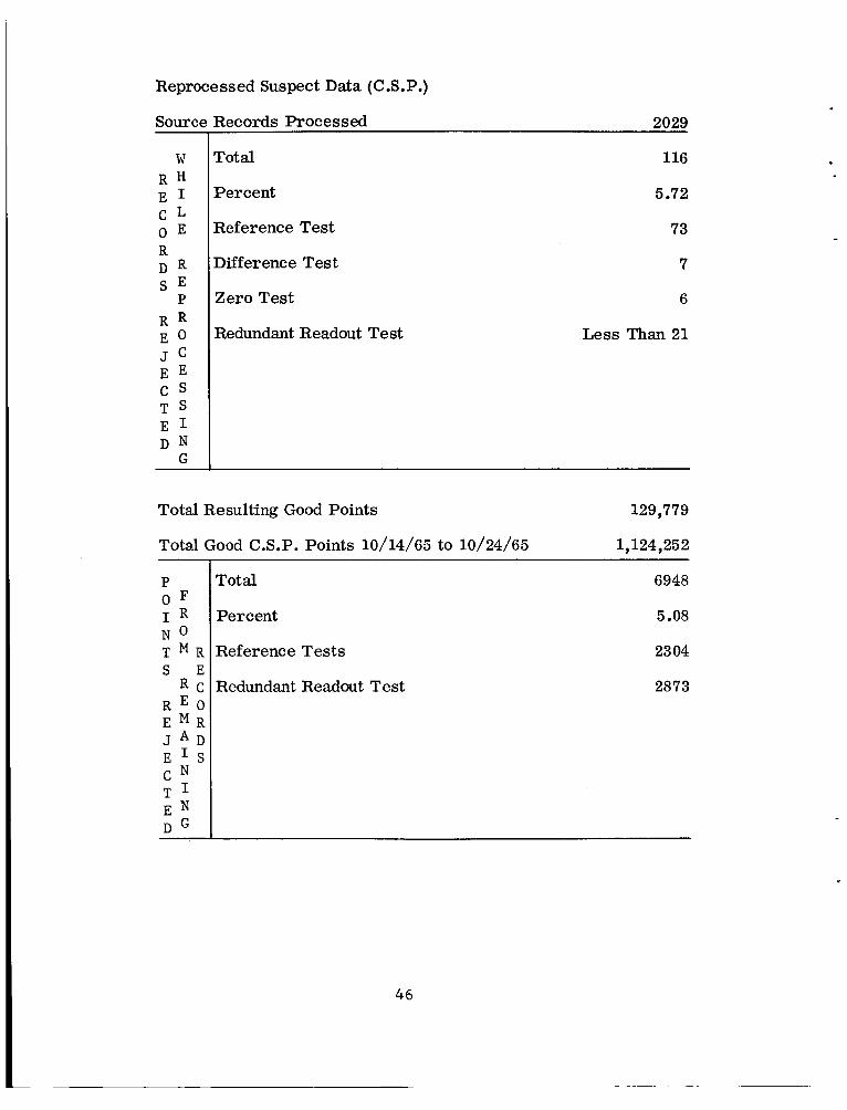
Reprocessed Suspect Data (C.S.P.)
Source Records Processed 2029 I
W R H E 1
Total
Percent
116
5.72
0 E Reference Test 73 c L I R D R
P R R E o J c E E
T S E 1 D N
G
S E
c s
Difference Test
Zero Test
Redundant Readout Test
7
6
Less Than 21
Total Resulting Good Points 129,779
Total Good C.S.P. Points 10/14/65 to 10/24/65 1,124,25 2
P O F I R
T M R
R C
N o
S E
R E O E M R J A D E ' S
T I E N D G
C N
Total
Percent
Reference Tests
Redundant Readout Test
6948
5.08
23 04
2873
46
I
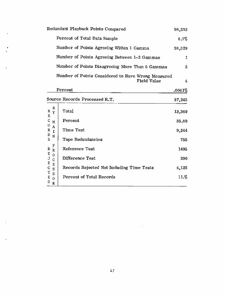
Redundant Playback Points Compared 98,333
8.7% Percent of Total Data Sample
Number of Points Agreeing Within 1 Gamma 98,329
1 Number of Points Agreeing Between 1-2 Gammas
Number of Points Disagreeing More Than 5 Gammas 3
Number of Points Considered to Have Wrong Measured Field Value 4
Percent .0041%
Source Records Processed R.T. 37,245
Total
Percent
Time Test
Tape Redundancies
13,369
35.89
9,244
755
Reference Test 1495
Difference Test 390
Records Rejected Not Including Time Tests 4,125
Percent of Total Records 11.%
47
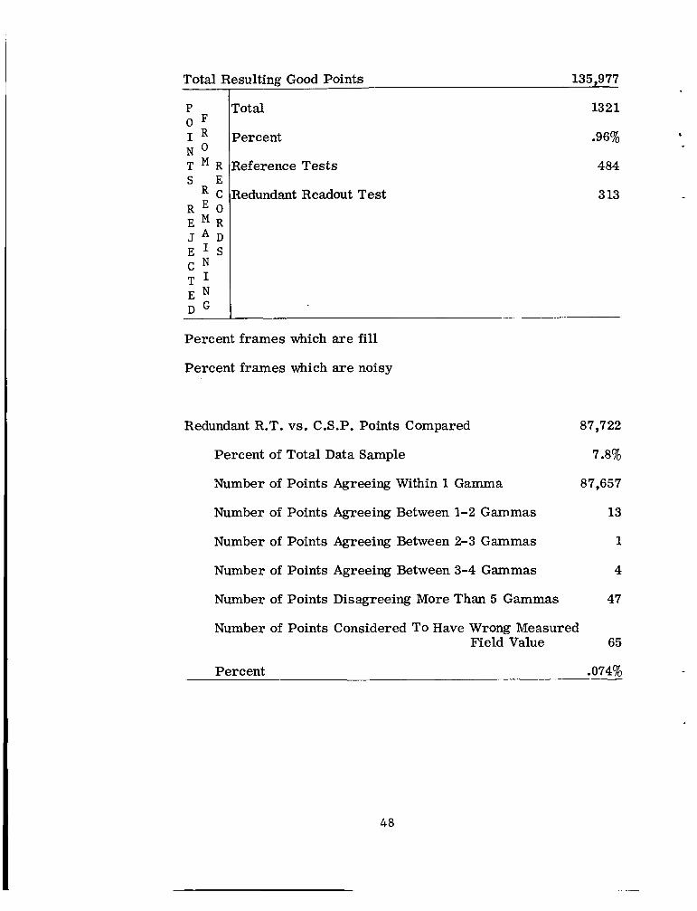
P O F I R N o T M R S E
R E O E M R J A D E ' S
T I E N D G
R C
C N
Total Resulting Good Points 135,977
rotal
Percent
Reference Tests
Redundant Readout Test
1321
36% . 484
3 13
Percent frames which are f i l l
Percent frames which are noisy
Redundant R.T. vs. C.S.P. Points Compared 87,722
Percent of Total Data Sample 7.8%
Number of Points Agreeing Within 1 Gamma 87,657
Number of Points Agreeing Between 1-2 Gammas 13
Number of Points Agreeing Between 2-3 Gammas 1
Number of Points Agreeing Between 3-4 Gammas 4
Number of Points Disagreeing More Than 5 Gammas 47
Number of Points Considered TO Have Wrong Measured Field Value 65
Percent .074%
48
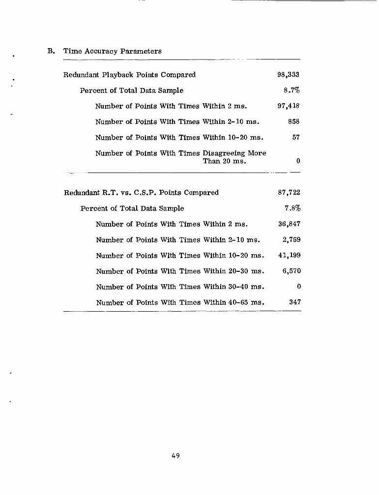
B. Time Accuracy Parameters
Redundant Playback Points Compared 98,333
8.7% Percent of Total Data Sample
Number of Points With Times Within 2 ms.
Number of Points With Times Within 2- 10 ms.
97,418
8 58
Number of Points With Times Within 10-20 ms. 57
Number of Points With Times Disagreeing More Than 20 ms. 0
Redundant R.T. vs. C.S.P. Points Compared
Percent of Total Data Sample
Number of Points With Times Within 2 ms.
Number of Points With Times Within 2-10 ms.
Number of Points With Times Within 10-20 ms.
Number of Points With Times Within 20-30 ms.
Number of Points With Times Within 30-40 ms.
Number of Points With Times Within 40-65 ms.
87,722
7 3%
36,847
2,759
4 1,199
6,570
0
347
49
reprocessed from each type of rejection. The records which are not completely
rejected still contain a certain percentage of suspect data. For this time period
this percentage was 1.04. The table shows this figure along with the number of
points in each of several main rejection categories. Comparable indications a re
available for the reprocessed data. While the statistics for entire records
rejected during reprocessing a re included in the Quality Summary, the numbers
a re not comparable to those from the main processor since the rejection criteria
have been relaxed. The percentage of suspect data from those records not com-
pletely rejected is still a good indicator. For the period 10/14-10/24, 1965, it
was 5.08%, five times the figure from the main processor. The reprocessed
data is, indeed, of substantially lower quality than the good data resulting from
the main processor. This means that a higher p2rcentage of data are likely to
be accepted as good when they are really spurious. A visual inspection of plots
produced by the suspect data reprocessor for the data from 10/14-10/24, 1965,
bears this out. We would estimate from .5 to 1% of the recovered data is spuri-
ous to some degree. These errors are usually less than 107’ but may occasionally
be lOOy or more. These points should be eliminated by the AF f i t test on the
analysis tape.
Because of the high percentage of spurious data placed on the good data tape
during reprocessing of suspect data, the n2w test described in Section 8 has been
added to the suspect data reprocessor. This test reduced the spurious points,
detected by visual inspection of the plots from the reprocessor, to less than 1/20
of one percent when the data from 10/29/65 to 11/15/65 were reprocessed. We
intend adding this test to the main processor in the near future.
50
The statistics from the real time data reveal a startling percentage of en-
t i r e records rejected. This is almost exclusively the result of inaccurate time.
Indeed when the rejections from the time tests a re not taken into account the
percentage rejection is within one percent of the similar figure for C.S.P. data.
The "time problem" will be discussed later in this section. The percentage
suspect data resulting from those records not completely rejected is also very
nearly the same as for C.S.P. We conclude that, aside from the time problem,
the C.S.P. and R.T. data are of comparable quality.
A good indicator of the amount of spurious data finding its way into the good
data tapes is obtained by comparing overlapping data. C.S.P. data overlaps
occur under two circumstances. Occasionally two telemetry stations a re able to
simultaneously receive the same telemetry from the spacecraft. Secondly, each
station usually records the telemetry on two recorders simultaneously. In
either case, i f the Telemetry Computation Branch processes both sources we
will have overlapping data. Another source of data overlap is when RT data and
CSP data a re taken simultaneously. Obviously there is a greater degree of in-
dependence in sources when RT is compared to CSP than when CSP is compared
to CSP.
The statistics from the overlap comparison are given in two parts in the
Quality Summary. First the CSP-CSP overlap and secondly the RT-CSP over-
lap. Both comparisons a re over a statistically significant percentage of the
data and both indicate less than .1% spuriow magnetic field values.
A s of this writing, complete analysis cleanup figures are not available.
Preliminary statistics from test runs of the analysis cleanup program indicate
that about .4% of the data is being removed from the analysis tape. This is not
51
unduly higher than the amount of spurious data found while comparing overlapping
data, and indicates that most of the spurious data a re being removed. A visual
inspection of data plots confirms this conclusion.
Because the times associated with the data a re derived from the time f i t ,
the accuracy of these times depends both upon the accuracy of the f i t itself and
on the accuracy to which the data time matches the time fit.
The time checks in the main processor a re all oriented toward assuring
that the data times match the time fit. These tests assure that i) at the start
of the file the data time matches the time fit to 26 milliseconds, and ii) the time
for each record matches the time at the start of the file to 44 milliseconds. We
are confident that almost all of the times on the data (over 95%) agree with the
time f i t to within 30 milliseconds. The possibility exists, however, that isolated
chunks of data will be up to 70 milliseconds different from the time expected on
the basis of the time fit.
For C.S.P. data after January 25, 1966 and R.T. data after November 19,
1965, the time for each record is compared to the time fit itself. An accuracy
of 26 milliseconds is required. This means that the maximum deviation of data
times from the time fit will be 26 ms.
When comparing overlapping data the times are compared as well as the
field values. The results of these time comparisons are shown in Part B of the
Quality Summary. For C.S.P. overlap with C.S.P. data all times were within
20 milliseconds and most were within 2 milliseconds, For R.T. overlapping
with C.S.P. there is a large group agreeing within 2 milliseconds and another
large group differing between 10 and 20 milliseconds. This unexpected time
difference is due to a constant bias of 18 milliseconds on the 64 K B real time
52
b
data, present on the source tapes received from the Telemetry Computation
Branch. Unfortunately the error was detected too late to correct the problem on
any data before August of 1966.
In spite of this bias all of the comparisons, except one small batch, agreed
to within 30 milliseconds. The small amount of data whose time er ror is about
66 ms, resulted from a small time error in a 64 KB file which went undetected
by our time check and amounts to .4% of the data compared.
We conclude that the bulk of the data in the analysis tapes (that which de-
rives from the C.S.P. data) has times agreeing to within 20 ms. of the time fit.
The remainder of the data agrees to within 30 ms. of the time fit with the ex-
ception of some small amounts which may be off up to 70 ms. Between 4-8% of
the data has a constant bias of 18 ms.
The accuracy of the time f i t is difficult to assess. The Control Equipment
Branch at GSFC (Laios -9 1967), who are responsible for the equipment at the
various ground stations, inform us that the station clocks can be synchronized
to within one millisecond of the received signal from WWV and that the master
oscillators at the stations are stable to better than one part in 10" per day.
This stability implies that once synchronization with WWV was attained many
days would have to pass before the station clock would differ more than a milli-
second o r two from WWV.
The time codes placed on the analog tape (See Section 4) should, therefore,
be accurate to rt2 ms. These time codes a re decoded by the STARS-I time de-
coder (Demmerle, 1964) with a resolution of l ms. and a precision of one ms.
Thus the claimed accuracy of the time into the time f i t program is better than
3 ms. Since the resolution of the clock update is *4 ms. (See discussion of
53
high resolution points, Section 6 , iv), the accuracy of the time f i t data should be
better than m, or better than 5 ms.
The only other inaccuracy in the data into the time f i t should be that of the
short term drift of the satellite clock. This is specified to be one part in l o 6 .
The long term drift of the clock should be accounted for by the time fit .
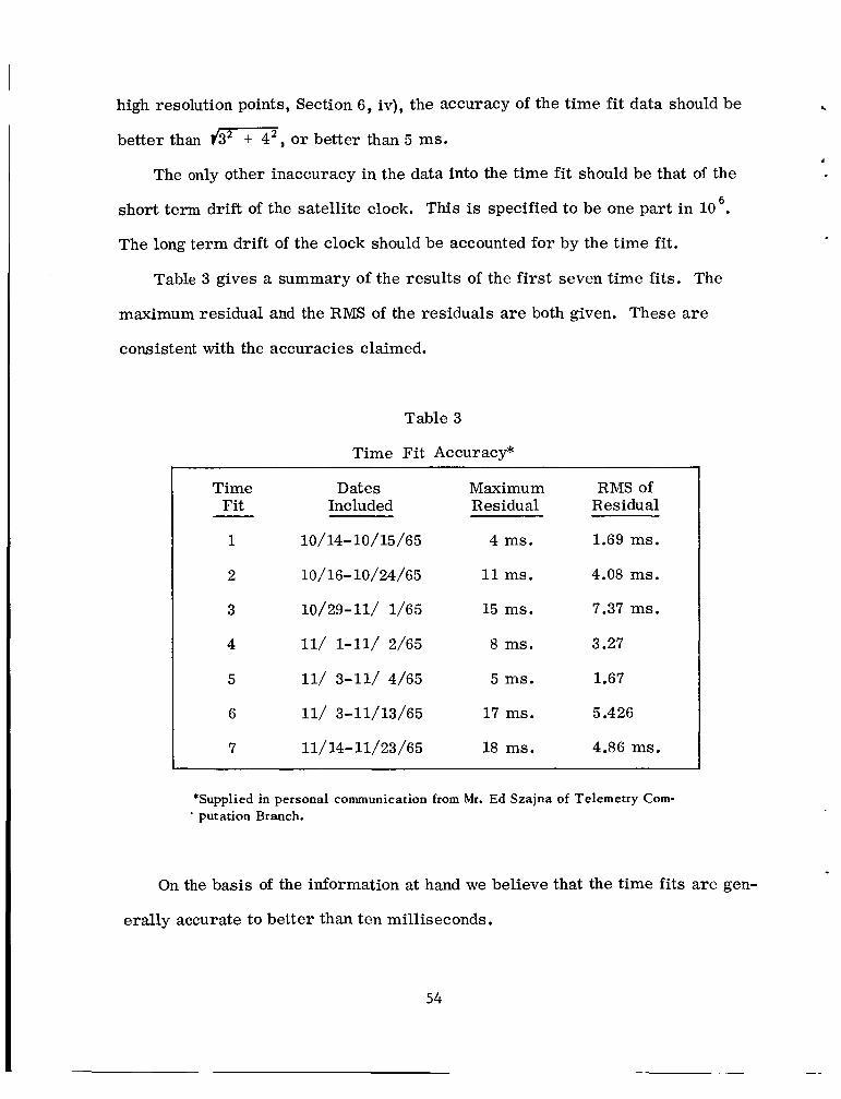
Table 3 gives a summary of the results of the first seven time fits. The
maximum residual and the RMS of the residuals are both given. These a re
consistent with the accuracies claimed.
Table 3
Time Fit Accuracy*
Time Fit
1
2
3
4
5
6
7
Dates Included
~
10/14- 10/15/65
10/16- 10/24/65
10/29-11/ 1/65
11/ 1-11/ 2/65
11/ 3-11/ 4/65
11/ 3-11/13/65
11/14-11/23/65
Maximum Residual
4 ms.
11 ms.
15 ms.
8 ms.
5 ms.
17 ms.
18 ms.
RMS of Res idu a1
1.69 ms.
4.08 ms.
7.37 ms.
3.27
1.67
5.426
4.86 ms.
*Supplied in personal communication from Mr. Ed Szajna of Telemetry Com- ’ putation Branch.
On the basis of the information at hand we believe that the time fits are gen-
erally accurate to better than ten milliseconds.
54
L
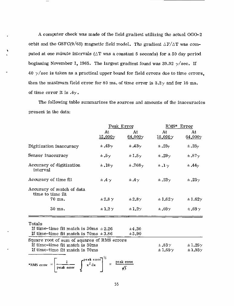
A computer check was made of the field gradient utilizing the actual OGO-2
orbit and the GSFC(9/65) magnetic field model. The gradient AF/AT was com-
puted at one minute intervals (AT was a constant 5 seconds) for a 50 day period
beginning November 1, 1965. The largest gradient found was 39.92 y/sec. If
40 y/sec is taken as a practical upper bound for field errors due to time errors,
then the maximum field e r ror for 8 0 ms. of time error is 3 . 2 ~ and for 10 ms.
of time error it is .4y.
The following table summarizes the sources and amounts of the inaccuracies
present in the data:
Digitization inaccuracy
Sensor inaccuracy
Accuracy of digitization interval
Accuracy of time fit
Accuracy of match of data
70 ms. time to time f i t
30 ms.
Peak Error At At
15.000~ 64.0 OOy
f .43 y f .43y
f.5y f 1 . 5 ~
f .18 y f ,768 y
f .4 y f .4y
f2.8 y f2.8Y
f 1.2 y f 1.2y
RMS* Error At At
15.000y 64. OOOy
f .25y f .25y
f'.29y f .87y
f . 1y -I .44y
f .23y f .23y
f 1.62 y f 1 . 6 2 ~
f .69y f .69 y
Totals If time-time fit match is 30ms f 2.26 If time-time fit match is 70ms f3.86
If time-time f i t match is 30ms
*4.30 f 5.90
Square root of sum of squares of RMS errors f .83y f 1.25 y
If time-time fit match is 70ms
*RMS error =
- peak error
fi 1
peak error
f 1.69 y f 1 . 9 3 ~
55
Taking all of the above error sources into account, both in the field value
and time value, we would (confidently) estimate the data on the final analysis
tape (with the possible exception of a few scattered points) to be better than
2.07, with the probable accuracy better than .83Y at 15,0007 and 1.257 at
64,0007.
12. DATA EXTENT
Figures 10 and I1 show the data coverage from OGO-2. Figure 10 is a plot
giving the geographical distribution of all playback data (both good and suspect)
for the time period 14-24 October, 1965. Altitude is not indicated but limited
altitude inferences may be drawn from the knowledge that perigee is in the
northern hemisphere (perigee varied from approximately 0" latitude to 30" lati-
tude during this period) and occurs at a local time of approximately 5 a.m.
(Langel, 1967).
The distribution of the data as a function of Universal Time is given in
Figure 11. This figure includes both C.S.P. and R.T. data (again both good and
suspect). The date is indicated on the ordinate, one horizontal line applying to
each day, and the Universal Time along the abscissa. Gaps occur where there
is no magnetic field data.
13. PROCEDURES IN DATA PROCESSING
From the very beginning of this effort our goal has been to supply the
analyst with data tapes containing - all of the good data but no spurious data.
This, of course, is a highly idealistic goal. The preceding sections of this
report (particularly Section 11 on Data Quality) should give the reader a fair
idea of our success in meeting our goal.
4
f
56
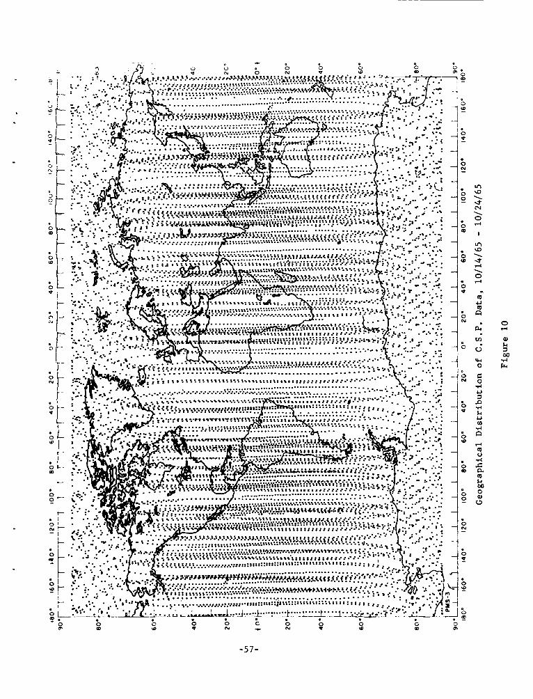
. e . . . . . 3 m
0 0 z s Q W 0 C N t
0 0
0 C 0 Q
0 E
* 0 E
0 9-
. 0 2
. 0 0
. 0 m
. 0 w
. 0 0
. 0 (u
0
::
b 0
0 Q
0 m
0 0
. 0 N -
0 0
0 ?
L z
->I-
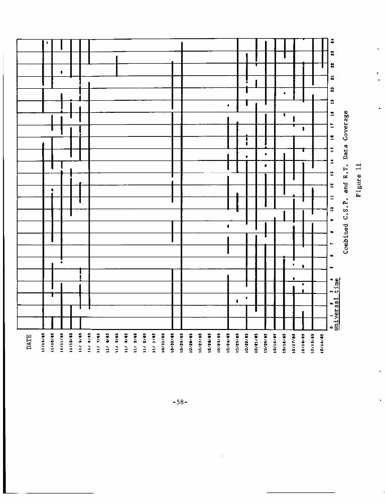
. -
I I -
I
-58-
In this section we briefly describe part of the rationale behind our methods
and some thoughts about how our procedures could be improved, both with exist-
ing computer hardware and with some of the new hardware currently being made
available.
One alternate approach to data processing would be to reformat the original
data into a format convenient to the analyst (including coordinate transforma-
tions, transformations into engineering units, etc.) and then construct an index
to the data for access purposes. This means that the analyst is left to determine
which data is suspect, to time order the data, and to eliminate redundant data.
Another extreme would be for the data processor to eliminate all data which he
(even remotely) suspects may be erroneous and make no attempt at recovery,
thus insuring only good data for analysis. Both of these approaches require a
minimum of programming, but neither approach satisfies our goals.
Because we wish to eliminate all spurious data, we have built extensive
"tests" into our processing programs s o a s to detect any data with a significant
probability of being erroneous. We had no inkling whatsoever, before launch, of
what forms the erroneous data would assume but hoped that the tests would prove
adequate without rejecting data needlessly. Not knowing how successful the
tests were going to be, we decided not to reject any data irretrievably but,
rather, to set it aside together with enough descriptive information to tell us
why it was considered suspect. This led to the "Suspect Data Tape."
We have tried to organize our data in its most useable form, that is, so
that a particular type of data appears in that format from which it may be most
easily accessed when being used in its most important application. The data
usages considered a re described in the following table:
59
Data Usage . Data Type
Suspect
Engineering
Good
Primary Use
Reprocessing and merge with good data
1. Indicate when data may be suspect
2. Evaluation of instrumenta- tion performed
Analysis of earth's mag- netic field
Secondary Uses
Evaluation of experiment instru- mentation and of telemetry digitization and processing procedures.
Correlation with unexplained phenomena during data analysis
Examination to assure accurate measurements.
With the primary usage of the final good data in mind we arrived at the
following criteria for our good data tapes:
1.
2.
3 .
They should be kept separate from the suspect and engineering data.
They should be as free as possible from suspect data.
The data should be grouped into time intervals such that all data from
a particular interval is contained on one and only one good data tape.
The source data comes to us in files, each of which has certain unifying
characteristics, such as data format and ground station at which recorded.
Within each file are sub-units called records, each containing data from one
spacecraft sequence. To maintain quick and ready reference to any portion of
the data, throughout most of the data reduction process, these units of data
organization have been maintained up until the time the analysis tapes are
formed. Thus there is a one to one correspondence between input files and
records and output file and records, except on the analysis tapes. This
60
e
organization enables US to examine data from particular stations, of particular
formats o r from particular tapes and/or runs from the Telemetry Computation
Branch . An alternate approach would have been to simply keep track of the source
tapes, files, and records on which suspect data occurs and go back to these
tapes for reprocessing. The arguments advanced for this are that it would in-
volve fewer overall tapes and that special programs to read the suspect tapes
would not be necessary. However, a typical time period (say 10/14-10/24/65)
to be processed (either for the first time or for reprocessing) will include from
40-80 source tapes. Some suspect data results from each of these tapes, always
including some entire records and sometimes some sizeable chunks. Re-
processing would rarely include less than 20 of these tapes, with bits and pieces
needed from each tape. In contrast, all of the suspect data from such a time
period can be contained on one suspect data tape.
Reprocessing with the main processor would require that the main processor
be able to access individual records on each input tape. On the other hand sub-
routines to access output data tapes (e.g. good data, engineering and housekeep
ing) normally have very flexible access capabilities. We have concluded that by
making our data access routine slightly more flexible (i.e. able to handle addi-
tional formats) and limiting our main processor routines so that they can only
pick-and-choose among files (instead of records also) does not really cost us
any programming effort and gives us far more flexibility in reprocessing sus-
pect data than we would have if we re-ran it through the main processor and, at
the same time, actually reduces the number of tapes necessary to handle during
reprocessing.
61
Another consideration in the problem of reprocessing suspect data is that if
reprocessing is done from the source tapes, all information regarding the
original rejection must be kept on the housekeeping tape, whereas if a new tape
is written flags may be mixed with the data to indicate why the data was con-
sidered suspect. These flags may then be used in reprocessing to help control
program decisions.
The programming effort to reprocess the data for the first ten days after
launch has been less than four man-months above what would have been required
if the suspect data had simply been ignored, The effort to extend reprocessing
to other periods of time will now simply consist of the time to make any pro-
gram changes necessary to cope with new situations not encountered with the
initial ten days data. The resulting program has a large amount of flexibility in
selecting data to be reprocessed; it can process entire files, groups of records,
or individual records. It is capable of plotting all or part of the data reproc-
essed during a run and may easily be modified to change data rejection criteria
from file to file. In operation the major portion of time probably is consumed
in remaking the housekeeping tape (to be discussed shortly) to indicate what has
been reprocessed with what results. This arrangement seems to give highly
satisfactory results.
We expect that the amount of data reprocessed from the suspect data tape
will drastically decrease in the near future. Reprocessing consists of putting
the data to the same tests as in the main processor, with different rejection
criteria, and of developing new tests as needed, under more closely controlled
(and monitored) conditions than is possible in the main processor. The obvious
62
next step is to modify the main processor in accordance with the new proce-
dures. This is being carried out successfully at the present time.
The housekeeping tape has proved invaluable as a detailed record of both
the main processing and suspect data reprocessing. We have often used it when
seeking to determine, in detail, the quality of data at a particular time or on a
particular file and record. It has been used to produce various types of data
summaries including the index tape, plots of data coverage (both spatial and
temporal) and summaries of data quality for given periods of time. While we
feel that this tape has proved very useful, hindsight tells us that it can be vastly
improved. Its initial generation costs very little either in programming effort
or in machine time. However, when reprocessing suspect data the entire house-
keeping tape must be rewritten to indicate that the initially rejected data has
been reprocessed and to describe the results of the reprocessing. This i s a bit
expensive in machine time.
The format of the housekeeping tape has proved more cumbersome and less
useful than originally intended. Substantial amounts of data render it too long to
be used as a rapid index to the other tapes and it contains too much information
for the quick, short, summaries which we have occasionally wanted. For future
efforts we feel that the file housekeeping should be expanded to where a set of
file housekeeping records will serve in place of our index tape. Such a set of
file housekeeping records should also provide a quick summary not only of what
files have been processed but also of the general quality of the results. At the
same time the record housekeeping should be contracted to the point where
sorting the housekeeping tape into time order is no longer a major undertaking.
63
Among the peripheral hardware being made available for the next generation
of computers are the removable "disk pack" and the data cell. Because these
devices are of the "direct access" type they have the potential to make data
access an order of magnitude simpler than tape systems, such as the one de-
scribed in this document. For example, the disk pack should be ideally suited
for containing housekeeping information. The data could still be grouped into
logical "files," one to one with input files. Two advantages a re immediately
obvious:
1. Since records can be updated in place (without disturbing their neigh-
bors; unlike tape), when suspect data is reprocessed it will not be
necessary to re-create the entire housekeeping data set.
Time ordering may be achieved without costly sort techniques by using
proper indexing and chaining techniques for the file level housekeeping.
2.
If the cost/data bit of the data cell can be made reasonable (say no more
than twice that of storing the same data on tape), then the data cell would offer
similar advantages for data storage as the disk pack for housekeeping storage.
14. DISCUSSION AND CONCLUSIONS
To those who have faced the data herein described since long before OGO-2
was launched, the characteristics of the data, even to the most minute detail,
seem very obvious. We hope that a good measure of this knowledge and experi-
ence is contained in the preceding sections. Our confidence in the quality of the
data being released to the NASA Space Science Data Center is very high.
While we feel that others should be able to profit from our efforts in data
processing, one should be aware of some of the unique features of this experi-
ment and this satellite before generalizing from our results to those from other
64
.
satellites and even from our experiment to others in the OGO satellites. This
experiment was probably the simplest in concept on OGG2. It sampled the main
scalar field at roughly equal intervals of one-half second regardless of the bit
rate and format (main comm. or flexible format) and with little concern for the
spacecraft attitude. The most serious problem encountered was that of identi-
fying the data with the appropriate Universal Time to an accuracy consistent
with the instrumentation accuracy.
We should note in retrospect that the OGO series is probably the most com-
plex and flexible satellite observatory ever to achieve any degree of success.
This complexity is multiplied in the low altitude, polar, half of the OGO series
by the complex scheduling problems caused by short (10-15 min) station passes,
and by the power problems caused by rapid cycling through eclipses when the
satellite leaves the twilight meridian. The satellite flexibility and complexity
(particularly the usage of flexible format) is more of a hindrance than a help for
this particular experiment and indeed makes the effort of data reduction many
times greater than for data recorded on a less complex system. This inherent
complexity, coupled with the intermittent operation of the spacecraft and with
the program problems in Telemetry Computation Branch's time correction, has
in fact raised the problems of processing and evaluating the data a good order of
magnitude over that which might have been achieved with a less ambitious
project.
As has been seen some of the system redundancy is helpful in gaining greater
confidence in the recorded results; most is not, The recording in real-time at
the receiving stations of data that are also recorded on board appears to be a
useful aid for cross comparison and for filling gaps in the recorded data. The
65
usefulness of the special purpose system, placed in operation partly as back up
to the main data recording system, has yet to be realized in providing additional
data information. Of course if the main recording system had failed, this docu-
ment would be discussing only the results from the special purpose telemetry.
66
ACKNOWLEDGMENTS
An effort of this magnitude necessarily involves many individuals. The over-
all project is under the direction of Dr. J. C. Cain who has given a great deal of
help in establishing our basic philosophy as well as guiding us in the selection
of data test criteria. Significant direct participation in the programming was
taken by Mr. Dean Wood (then with Aero Geo Astro Corp.), Mr. W. Jungemeyer
and Mr. L. Karleson (then with Computer Sciences Corp.). I must also
acknowledge the valuable advice of Miss S. Hendricks (of GSFC), Mr. L.
McCarter (of New Mexico State University) and Mr. J. Premeaux (of Vitro
Services, Inc.).
67
REFERENCES
Cain, J. C., S. Hendricks, W. E. Daniels, and D. C. Jensen, Computation of the
Main Geomagnetic Field From Spherical Harmonic Expansions, GSFC
Report X-611-64-316, 1964.
Cain, J. C., R. A. Langel, and S. J. Hendricks, First Magnetic Field Results
from the OGO-2 Satellite, GSFC Report X-612-66-305, 1966.
Caughey, Robert T., and John J. Quann, Data Processing Plan for Polar Orbiting
Geophysical Observatory, GSFC Report X-564-65-329, August 1965.
Demmerle, A. M., T. J. Karras, W , H. Stallings, P. J. McCeney, G. W. Nooger,
and E. J. Lenart, Instruction Manual for the Time Decoder of the Satellite
Telemetry Automatic Reduction System (STARS), Data Instrumentation
Development Branch, Data Systems Division, Goddard Space Flight Center,
GSFC Report X-544-64-69, January 1964.
Farthing, W. H., and W. C. Folz, A Rubidium Vapor Magnetometer for Near
Earth Orbiting Spacecraft, GSFC Report X-612-66-575, December 1966.
Glaser , P. F., The Orbiting Geophysical Observatory Communication and Data
Handling Subsystem, Procedures of the 1962 National Telemetering Con-
ference, Volume 2, Paper 3-3.
Laios, S., Personal Communication, April 1967.
Langel, R., A Representation of the Perigee Motion of a Satellite As a Function
of Local Time, GSFC Report X-612-67-34, February 1967.
Ludwig, G. H., The Orbiting Geophysical Observatories, Space Science Reviews,
Vol. II, No. 2, August 1963.
Ludwig, G. H. (editor), OGO Program Bibliography, National Space Science Data
Center, September 30, 1966.
68
Sarles, L. R., Varian Associates, Personal Communication to Mr. Winfield H.
Farthing, October 1966.
I -------- , NASA-GSFC Operations Plan 10-65, Orbiting Geophysical Observatory
OGO-C, GSFC Report X-513-65-346, August 1965.
-------- , The Orbiting Geophysical Observatories, Brochure for Experimenters,
GSFC, December 196 1.
69
APPENDIX A: Tape Formats
The following pages contain a detailed description of the formats of our
more important tapes. These include the analysis tape, housekeeping tape,
subcom-amplitude tape (engineering information), and the good data tape. All
of these, except the analysis tape, begin with a one file, one record, tape label
which is also described. Section 7 of this document should be consulted for
further explan at ion.
70
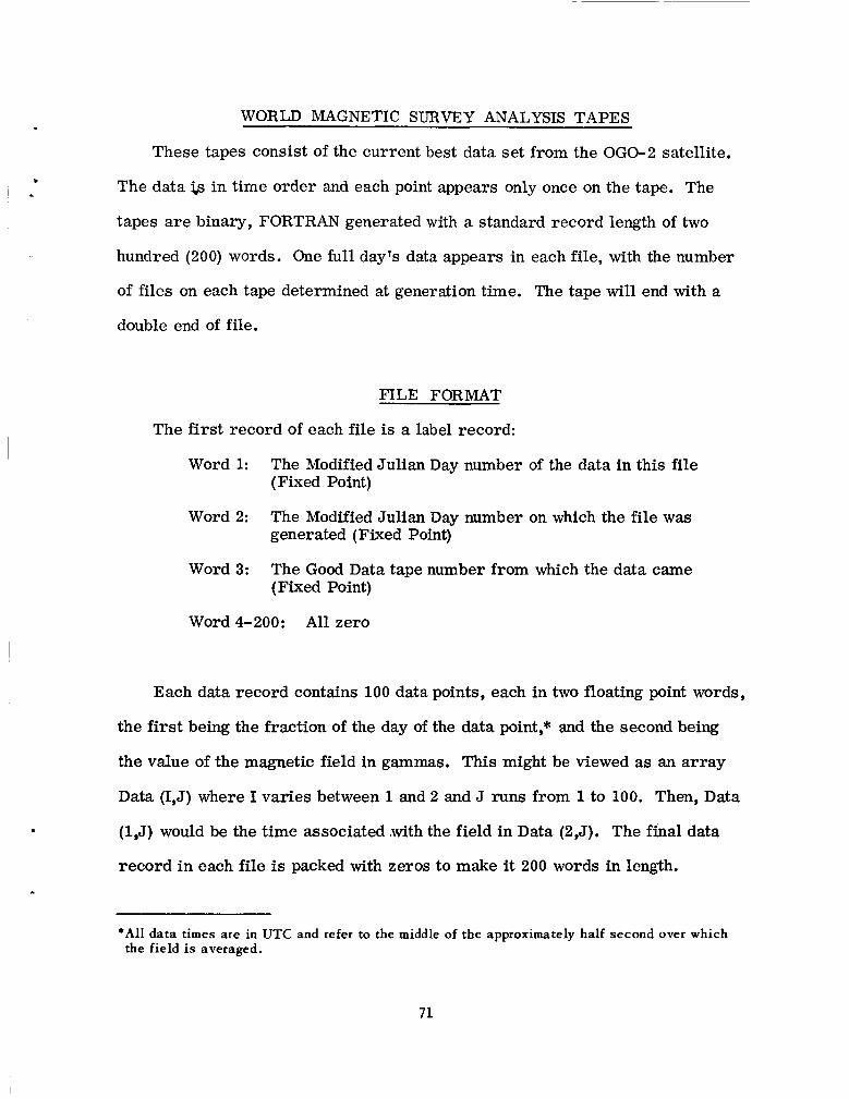
l -
i b
I .
WORLD MAGNETIC SURVEY ANALYSIS TAPES
These tapes consist of the current best data set from the OGO-2 satellite.
The data i,s in time order and each point appears only once on the tape. The
tapes a re binary, FORTRAN generated with a standard record length of two
hundred (200) words. One full day's data appears in each file, with the number
of files on each tape determined at generation time. The tape will end with a
double end of file.
FILE FORMAT
The first record of each file is a label record:
Word 1: The Modified Julian Day number of the data in this file (Fixed Point)
Word 2: The Modified Julian Day number on which the file was generated (Fixed Point)
Word 3: The Good Data tape number from which the data came (Fixed Point)
Word 4-200: All zero
Each data record contains 100 data points, each in two floating point words,
the first being the fraction of the day of the data point,* and the second being
the value of the magnetic field in gammas. This might be viewed as an array
Data (1,J) where I varies between 1 and 2 and J runs from 1 to 100. Then, Data
(1,J) would be the time associated .with the field in Data (2,J). The final data
record in each file is packed with zeros to make it 200 words in length.
"'All data times are in UTC and refer to the middle of the approximately half second over which the field i s averaged.
71
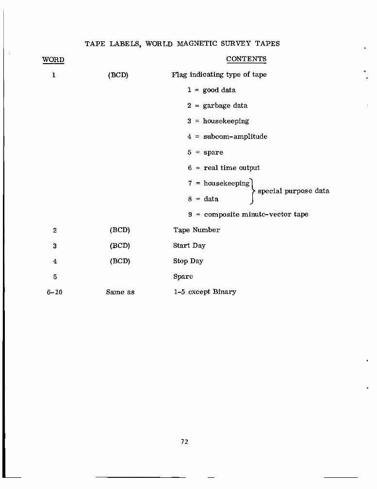
TAPE LABELS, WORLD MAGNETIC SURVEY TAPES
WORD CONTENTS
1 (BCD) Flag indicating type of tape
1 = gooddata
2 = garbage data
3 = housekeeping
4 = subcom-amplitude
5 = spare
2
3
4
5
6- 10 Same as
6 = real time output
7 = housekeeping special purpose data
8 = data 1 9 = composite minute-vector tape
Tape Number
Start Day
Stop Day
Spare
1-5 except Binary
72
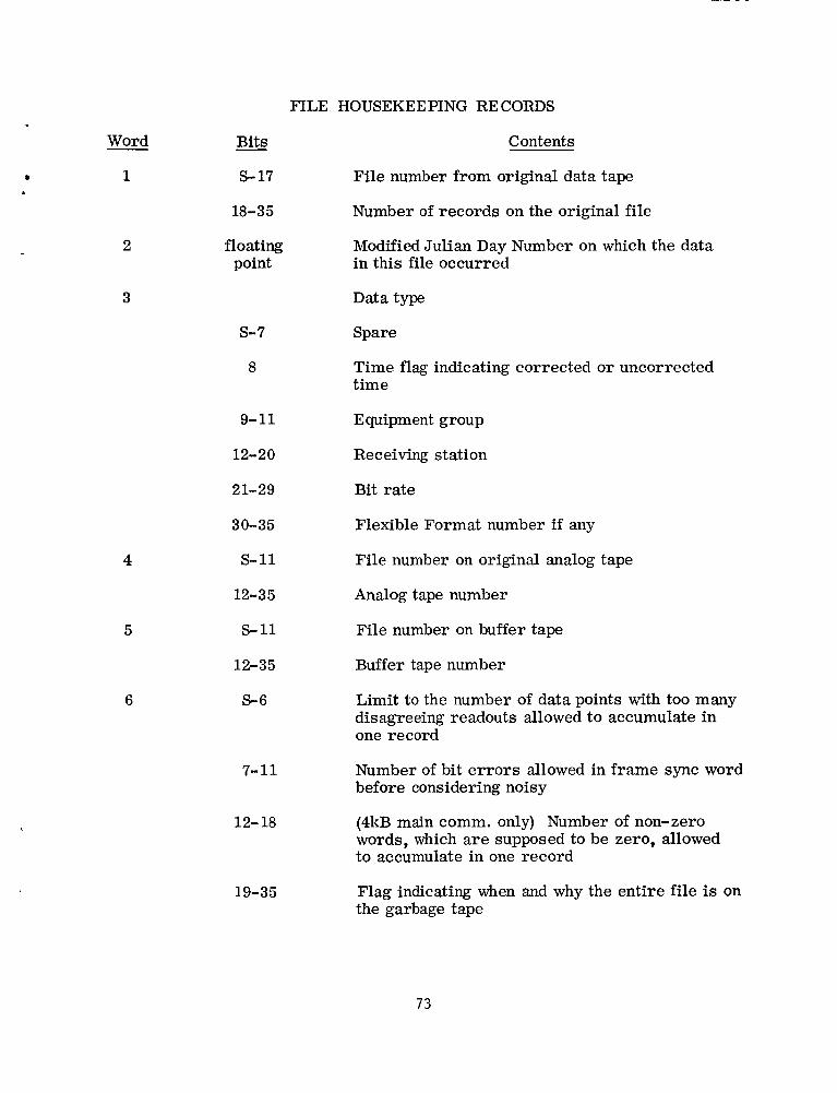
FILE HOUSEKEEPING RECORDS
8
Word
1
2
3
4
Bits
S- 17
-
18-35
floating point
s- 7
8
9- 11
12-20
21-29
30-35
$11
12-35
s- 11
12-35
$6
7-11
12- 18
19-35
Contents
File number from original data tape
Number of records on the original file
Modified Julian Day Number on which the data in this file occurred
Data type
Spare
Time flag indicating corrected or uncorrected time
Equipment group
Receiving station
Bit rate
Flexible Format number if any
File number on original analog tape
Analog tape number
File number on buffer tape
Buffer tape number
Limit to the number of data points with too many disagreeing readouts allowed to accumulate in one record
Number of bit errors allowed in frame sync word before considering noisy
(4kB main comm. only) Number of non-zero words, which a re supposed to be zero, allowed to accumulate in one record
Flag indicating when and why the entire file is on the garbage tape
73
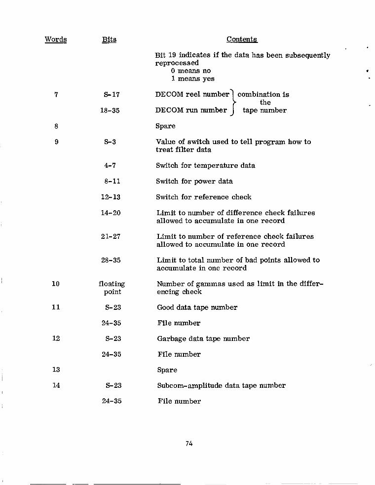
- Bits Contents Words
Bit 19 indicates if the data has been subsequently reprocessed
0 means no 1 means yes
DECOM reel number combination is
DECOM run number tape number
Spare
} the 7 S- 17
18-35
8
9 Value of switch used to tell program how to treat filter data
5-3
4-7
8-11
12- 13
14- 20
Switch for temperature data
Switch for power data
Switch for reference check
Limit to number of difference check failures allowed to accumulate in one record
Limit to number of reference check failures allowed to accumulate in one record
2 1-27
Limit to total number of bad points allowed to accumulate in one record
28-35
10
11
floating point
Number of gammas used as limit in the differ- encing check
S- 23 Good data tape number
24-35 File number
12 S- 23
24-35
Garbage data tape number
File number
13
14
Spare
5-23
24-35
Subcom-amplitude data tape number
File number
74
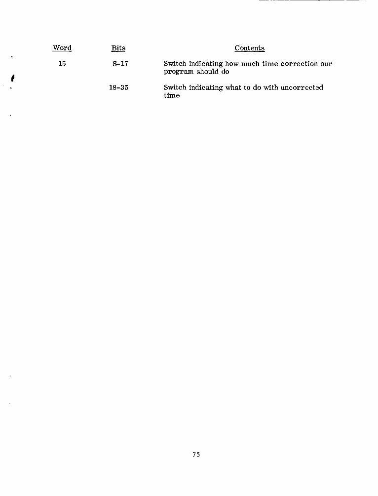
Word
15
- Bits C ont ent s
S- 17 Switch indicating how much time correction our program should do
18-35 Switch indicating what to do with uncorrected time
75
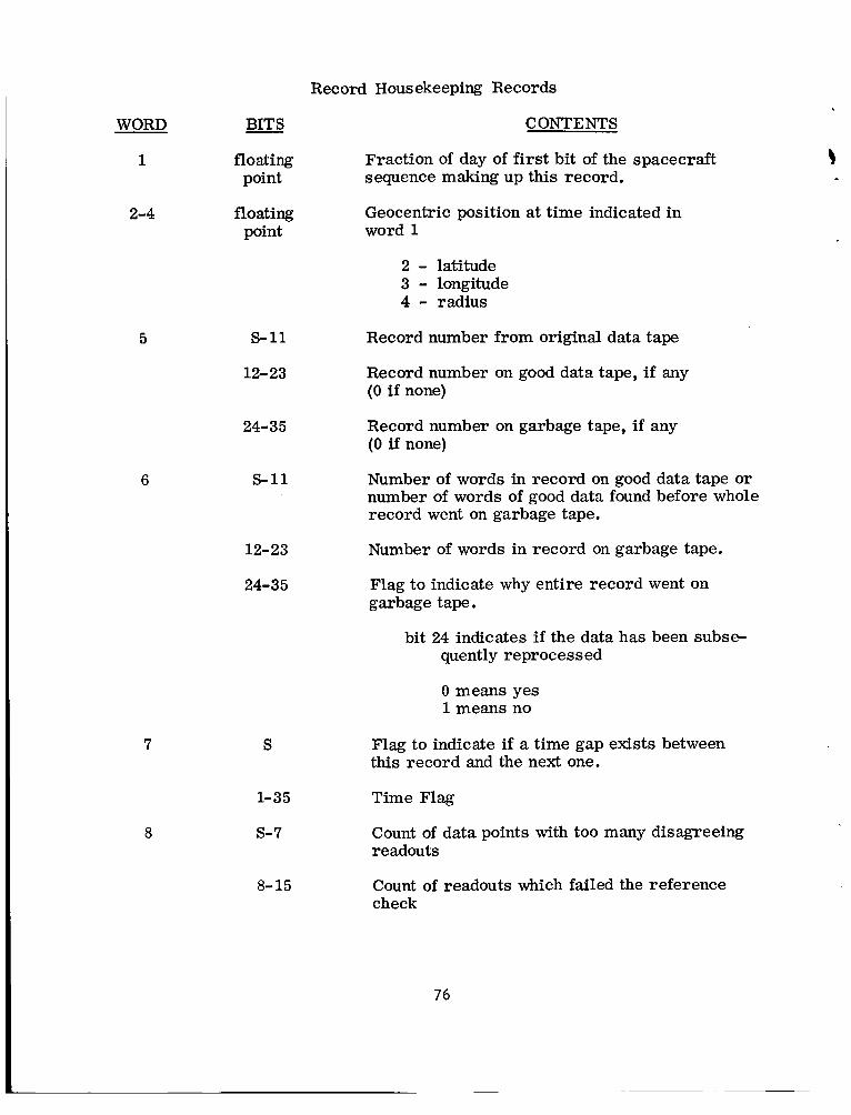
Record Housekeeping Records
WORD
1
2-4
5
6
7
8
BITS CONTENTS
floating point
Fraction of day of first bit of the spacecraft sequence making up this record.
floating Geocentric position at time indicated in point word 1
s- 11 12- 23
24-35
s-11
12-23
24-35
S
1-35
s- 7
8- 15
2 - latitude 3 - longitude 4 - radius
Record number from original data tape
Record number on good data tape, if any (0 i f none)
Record number on garbage tape, if any (0 if none)
Number of words in record on good data tape or number of words of good data found before whole record went on garbage tape.
Number of words in record on garbage tape.
Flag to indicate why entire record went on garbage tape.
bit 24 indicates i f the data has been subse- quently reprocessed
0 means yes 1 means no
Flag to indicate if a time gap exists between this record and the next one.
Time Flag
Count of data points with too many disagreeing readouts
Count of readouts which failed the reference check
76
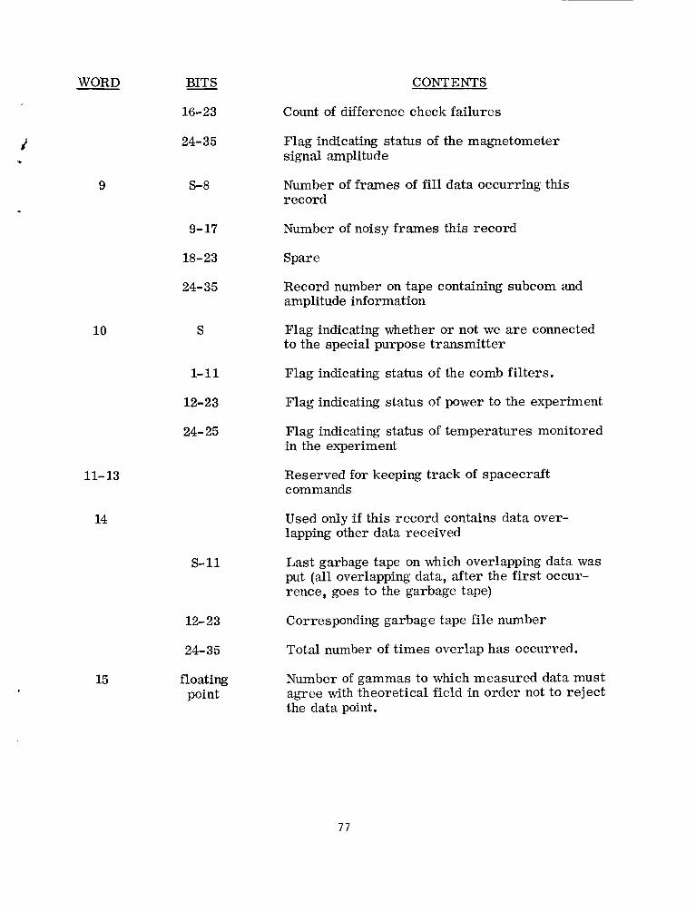
WORD BITS
16-23
24-35
9
10
11- 13
14
15
S-8
9- 17
18-23
24-35
S
1-11
12-23
24- 25
CONTENTS
Count of difference check failures
Flag indicating status of the magnetometer signal amplitude
Number of frames of f i l l data occurring this record
Number of noisy frames this record
Spare
Record number on tape containing subcom and amplitude information
Flag indicating whether or not we are connected to the special purpose transmitter
Flag indicating status of the comb filters.
Flag indicating status of power to the experiment
Flag indicating status of temperatures monitored in the experiment
Reserved for keeping track of spacecraft commands
Used only i f this record contains data over- lapping other data received
s-11 Last garbage tape on which overlapping data was put (all overlapping data, after the first occur- rence, goes to the garbage tape)
12- 23 Corresponding garbage tape file number
24-35 Total number of times overlap has occurred.
floating point
Number of gammas to which measured data must agree with theoretical field in order not to reject the data point.
7 7
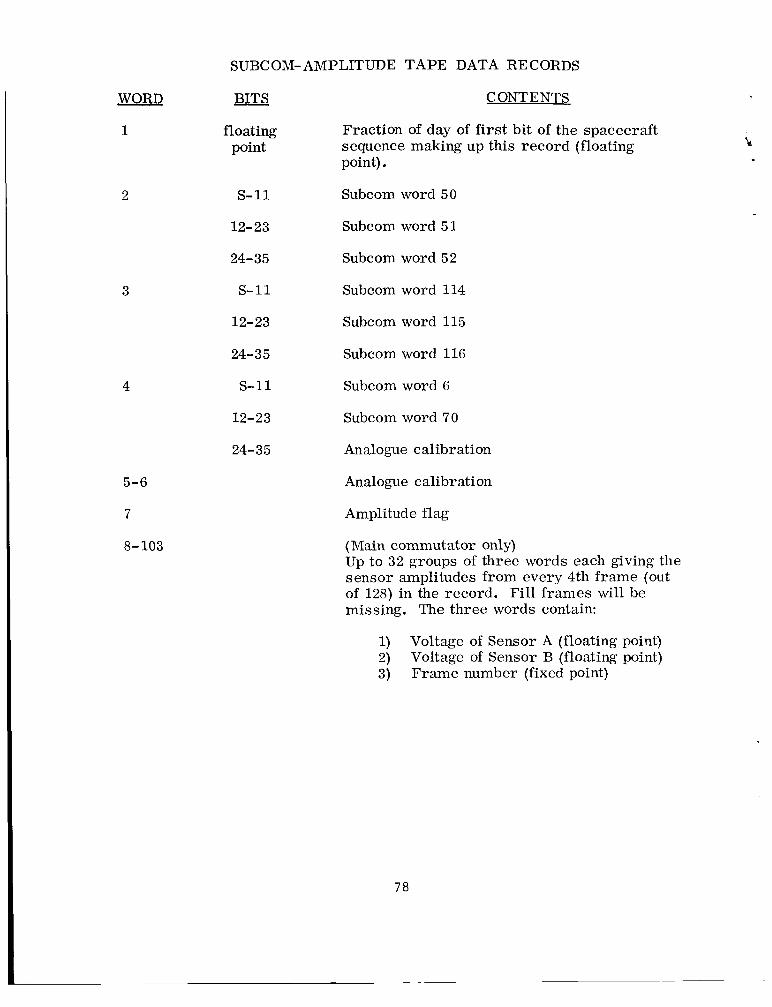
.WORD
1
2
3
4
5-6
7
8- 103
SUBCOM-AMPLITUDE TAPE DATA RECORDS
BITS
floating point
s-11 12-23
24-35
s-11 12-23
24-35
s-11 12-23
24-35
CONTENTS
Fraction of day of first bit of the spacecraft sequence making up this record (floating point).
Subcom word 50
Subcom word 51
Subcom word 52
Subcom word 114
Subcom word 115
Subcom word 116
Subcom word G
Subcom word 70
Analogue calibration
Analogue calibration
Amplitude flag
(Main commutator only) Up to 32 groups of three words each giving the sensor amplitudes from every 4th frame (out of 128) in the record. Fill frames will be missing. The three words contain:
1) 2) 3) Frame number (fixed point)
Voltage of Sensor A (floating point) Voltage of Sensor B (floating point)
78
&
Good Data Tape Data Records
These tapes have variable length records, not exceeding 148 words and
always containing an even number of words.
Two floating point words a re present for each data point, 1) the time, in
fraction of day, at the center of the counting interval for the data point and
2) the field value derived from the count.
7 9