Oklahoma Water Resources Research InstituteAnnual Technical Report

FY 2007

Oklahoma Water Resources Research Institute Annual Technical Report FY 2007 1

Introduction

This year, the Environmental Institute at Oklahoma State University was renamed the Institute for SustainableEnvironments, or ISE (pronounced “ice”). While the mission of the Institute has not changed, the new namereflects the emphasis on sustainability that has been characteristic of the Institute since Dr. Will Focht becamedirector in 2002. ISE continues to promote interdisciplinary environmental research, graduate education, andpublic outreach leading to better understanding, protecting, and sustainably developing the naturalenvironment. The Oklahoma Water Resources Research Institute (OWRRI) is located within the ISE and isresponsible for developing and coordinating water research funding to address the needs of Oklahoma. Toguide it in meeting this objective, the OWRRI has assembled a board of state regulators, policymakers, andother water resource professionals. This board is known as the Water Research Advisory Board (WRAB).

Introduction 1

Research Program Introduction

In 2007, proposals were solicited from all comprehensive universities in Oklahoma. Proposals were receivedfrom Oklahoma State University and the University of Oklahoma. Fourteen proposals were submitted andfrom these three projects were selected for funding for one year each.

− An Assessment of Environmental Flows for Oklahoma (Dr. Bill Fisher, OSU) uses the HydroecologyIntegrity Assessment Process (HIP) developed by the U.S. Geological Survey to assess environmental flowsin Oklahoma's perennial streams.

− Evaluation of Water Use Monitoring by Remote Sensing ET Estimation Methods (Dr. Yang Hong, OU)evaluates and improves remote sensing ET estimation methods and adapts them for use in Oklahoma.

− Decision Support Model for Evaluating Alternative Water Supply Infrastructure Scenarios (Dr. BrianWhitacre, OSU) will develop a step−by−step procedure that rural water systems can follow to assess theirwater supply infrastructure needs and will further assist in planning and locating funding for neededimprovements.

The final technical reports for these projects will be included in the 2008 Annual Report. The three technicalreports included herein are for the projects completed in 2007. All were granted extensions due to delays infunding during 2007, so only interim reports are provided below. Final technical reports will be submitted toOWRRI in the fall of 2008 and included in the 2008 Annual Report.

Research Program Introduction 1

Decision Support Model for Optimal Water Pricing Protocolfor Oklahoma Water Planning: Lake Tennkiller Case Study

Basic Information

Title:Decision Support Model for Optimal Water Pricing Protocol for OklahomaWater Planning: Lake Tennkiller Case Study

Project Number: 2007OK78B

Start Date: 3/1/2007

End Date: 2/28/2008

Funding Source:104B

Congressional District:3

Research Category:Social Sciences

Focus Category:Economics, Surface Water, Water Use

Descriptors:Water Supply, Water Use, Nonmarket Valuation of Water, Rural WaterDistricts

Principal Investigators: Tracy Boyer, Larry Sanders, Arthur Stoecker

Publication

Decision Support Model for Optimal Water Pricing Protocol for Oklahoma Water Planning: Lake Tennkiller Case Study1

Interim Technical Report Decision Support Model for Optimal Water Pricing Protocol for Oklahoma Water Planning: Lake Tenkiller Case Study Tracy Boyer, Arthur Stoecker, and Larry Sanders, Dept. of Agricultural Economics, Oklahoma State University

Objectives The objective of this study has been to develop a water pricing model that could be used

in the state water planning process. The model considers both monetary and opportunity costs in the allocation of surface water between competing uses. The model is being constructed for the Tenkiller Ferry Lake in Sequoia and Cherokee counties. The specific purpose is to develop a water pricing protocol that

(1) internalizes monetary and opportunity costs of water storage, treatment, and delivery systems; and

(2) generates an sustainable supply of water over the 2010-2060 period. Background

The lake dam is located in the Arkansas River Basin on the Illinois River in Sequoyah County. The lake is among the Oklahoma’s 34 major reservoirs that store 13 million acre-feet of water. The structure was federally authorized for flood control and hydroelectric power. Construction was completed by the US Army Corps of Engineers (USACE) in 1953. The lake has 130 miles of shoreline with a mean depth of 51 feet. Capacity is 654,100 acre feet at the normal pool and 1,230,800 at the flood pool (OWRB Fact Sheet). The main beneficial uses of the lake are recreation, flood control, power generation, stream flow maintenance and municipal and industrial use. The need for an economic model that optimizes net benefits from multiple water uses and tracks water balances for Tenkiller and other lakes is illustrated by statements from the U.S. Army Corps of Engineers (USACE) 2001 report on a proposed water treatment and conveyance study (USACE, 2001). According to the 2001 USACE report Lake Tenkiller had water rights of 29,792 acre feet with 14,739 feet allocated. Applications were pending for 172,714 acre feet. The USACE report found the 9,096 acre feet of water rights owned by the participating systems are insufficient to meet demands by the year 2050. The report further pointed out that “..having sufficient water rights does not guarantee a …. system would have enough water to meet projected demands. Water storage must also be considered”

Methodology:

Preliminary model On an annual basis a multiple use model of the lake is to maximize net benefits from market and non-market products. Net Benefits are measured in terms of Consumers’ Surplus + Producers’ Surplus + Net Government Revenue. The model can be stated as Max TNB = Σm ( BMm, BFm, BPm, BRm, BSm) Subject to Afm+1 = Afm + Inm – Rlm – Prm – MIm – Evm Afm < Vmaxm Afm > Vminm Where the value variables are

BMm is the average benefit from municipal and industrial use in month m. BFm is the average flood control benefit in month m, BPm is the average power generation in month m, BRm is the average recreational benefit in month m, and PSm is the average downstream benefit from releases in month m. Where the monthly quantity variables (measured in acre) are: Afm is the volume of water in the lake in month m, Inm is the inflow of water into the lake in month m, Rlm is the amount or water released for reasons other than power generation in month m, Prm is the amount of water released for hydropower in month m, MIm is the amount of water withdrawn for municipal and industrial use in month m, Evm is amount of water lost from evaporation and seepage in month m, and Vmaxm and Vminm are monthly maximum and minimum volumes in month m. The multiperiod model is obtained by expanding the annual model and by linking the end of year volume of the lake to the beginning volume for the next year. Future net-benefits are discounted. Rural Water System Simulation Models A hydraulic simulation model for a water system is a key tool that can be used to assist rural water districts (RWDs) in long term planning. In general, construction of these models can be expensive, time consuming and out of the reach of smaller RWDs. This study takes advantage of the Oklahoma Rural Water Systems GIS (geographical information systems) data set developed by the Oklahoma Water Resources Board (OWRB) which contains pipelines, facilities and general system capacity information. The available GIS files contain data on the length and diameter of each pipeline. The pipeline shape files have been overlaid on USGS 1/3 second elevation files. This step gives provides elevation data at points along the pipelines which is essential for estimation of pumping costs. Software programs have been developed to help with editing the apparently unused data set. Editing problems include missing pipes, mislabeled pipes, duplicate pipes, and duplicate nodes. Once the data files have been edited, input file to EPANET is generated. The simulation model is capable of estimating pressure zones and system performance under various population levels and spatial distributions of that population. The pressure zone data over the area served by a system under alternative population levels can be used to estimate costs for capital investments in pipelines and water treatment facilities. Pipeline files, district boundary files, facility files, and management files have been downloaded, for the water systems below. Burnt Cabin Cherokee County Rural Water District(RWD) #1 Cherokee County RWD #2 (Keys) Cherokee County RWD #3 Cherokee County RWD #7 Cherokee County RWD #8 Cherokee County RWD #13 (Cookson) City of Sallisaw East Central Oklahoma Water Authority Fin and Feather Water Association Lake Tenkiller Harbor Lost City RWD Muskogee County RWD #4 Muskogee County RWD #7 Paradise Hills, Inc. Sequoyah County Water Association Sequoyah County RWSG & SWMD #7 Stick Ross Mountain Water Company Summit Water Tahlequah Public Works Lake Region Electric Development Tenkiller Aqua Park Tenkiller State Park Town of Gore Town of Muldrow Town of Roland

Town of Vian Valuation of Recreational Goods Recreational Value of Lake Tenkiller is being estimated as part of a larger random utility travel cost model for all lakes in Oklahoma. The value or “price” of the trip is the travel cost to a site given its amenities and those of other substitute sites. A survey was distributed (26% return rate) to a random sample (proportional to the population in each county) of 2000 Oklahomans in late summer 2007 to collect information for travel cost and discrete choice models. Estimation of the trips taken as a function of the fee and lake levels is derived from Roberts et al (forthcoming 2008) to be fed into the optimization model outlined above. Preliminary results from the survey were presented at the 2008 Oklahoma Clean Lakes Association annual meeting.

Principal Findings and Significance:

Preliminary modeling for the optimization of water use is complete. However, completion of the rural water systems is ongoing as explained below. Data on recreational use is near completion for use in the model and independent data on recreational value of lakes throughout Oklahoma has been obtained as well. Data on system flows has been gathered and is ready for use in the modeling process. Finally, extension of results of research has met proposed goals, but will continue past the life of the project with the final results as explained below.

Work is continuing to complete development of the more than twenty RWS systems that

could be potentially served by water from Lake Tenkiller. Initial EPANET models have been completed for Cherokee County RWD#3, Tahlequah Public Works, Stick Ross Mountain Water Company.. Experience gained in completing the initial models has led to a better understanding of the problems involved. Software revisions to overcome these problems have been made and will continue to evolve. Data from a survey of RWD’s in the area will be used to improve the models. The EPANET program is used in this study because it is free, publically available, and can be given to cooperating RWDS to serve as a planning tool once the study has been completed.

Recreational values from the preliminary estimates of the discrete choice experiments

show that on average users visit Lake Tenkiller 4.7 times per year and value water quality at $8.75 per trip per increase in one foot of clarity. Lake users of Oklahoma lakes value water clarity, however, on average, they value amenities such as flush toilets and campsites with electricity at a much higher per trip rate. Boat ramps and portable restrooms were not significantly valued. Results from the travel cost model are forthcoming. Extension of Research Results Results from the recreational survey were presented at the Oklahoma Clean Lakes and Water Association meeting in Tulsa, Ok from April 9-11, 2008 to individuals from state agencies, volunteer environmental groups, and academics. An inservice workshop in Kellyville, OK, provided an opportunity for delivery of Lake Tenkiller research findings to OCES professionals from the counties in and around the Lake Tenkiller area. The program included presentations on:

1. Current water rights and law, and the potential for changes as the Comprehensive State Water Plan is underway;

2. The economics of water use in Oklahoma, including the Tenkiller region; 3. A comparison of water rates by selected water district; 4. Lake and river recreation and non-market valuation in the Tenkiller area. These presentations stimulated discussion on competing uses for the region’s water resources, as well as the need for further research and development of extension and outreach programs. As a result, several activities are planned: 1. A survey of the rural water districts in the Tenkiller to determine the factors that affect

water rates; 2. Meetings with the water districts and the public to discuss results of the Boyer, Stoecker,

Sanders research, and the water rates survey results; 3. Development of fact sheets, other educational materials, a website and public meetings to

address the perceived needs of county educators. 4. Further research and extension projects and proposals to follow up on questions this

research indicated a need for further study.

References:

Roberts, David, Tracy Boyer, and Jayson Lusk. 2008. Environmental Preferences Under Uncertainty. Ecological Economics (forthcoming 2008)

Mahasuweerachai, Phumsith. Essays on Recreational Valuations, Ph.D. Dissertation, Edmond Low Library, Oklahoma State University, Expected December, 2008.

Subsurface Transport of Phosphorus to Streams: APotential Source of Phosphorus not Alleviated by BestManagement Practices

Basic Information

Title:Subsurface Transport of Phosphorus to Streams: A Potential Source of Phosphorus notAlleviated by Best Management Practices

Project Number: 2007OK79B

Start Date: 3/1/2007

End Date: 2/28/2008

Funding Source:104B

CongressionalDistrict:

3 &2

Research Category:Ground−water Flow and Transport

Focus Category:Water Quality, Nutrients, Groundwater

Descriptors:Ground Water, Phosphorus, Preferential Flow, Riparian Floodplain, SubsurfaceTransport

PrincipalInvestigators:

Garey Fox, Glenn Brown, Chad Penn

Publication

Fuchs, J.W., G.A. Fox, D.E. Storm, C. Penn, and G.O. Brown. Subsurface transport of phosphorus inriparian floodplains: Influence of preferential flow paths. Journal of Environmental Quality (InReview).

1.

Fuchs, J.W., G.A. Fox, D. Storm, C. Penn, and G.O. Brown. 2008. Subsurface transport ofphosphorus in riparian floodplains: Tracer and phosphorus transport experiments. ASABE Paper No.084614. St. Joseph, Mich.: ASABE.

2.

Subsurface Transport of Phosphorus to Streams: A Potential Source of Phosphorus not Alleviated by Best Management Practices1

FY 2007 Oklahoma Water Resources Research Institute Grant Interim Technical Report

Title:

Subsurface Transport of Phosphorus to Streams: A Potential Source of Phosphorus not Alleviated by Best Management Practices (BMPs)

Garey A. Fox, Ph.D., P.E., Department of Biosystems and Agricultural Engineering, Oklahoma State University;

Daniel E. Storm, Ph.D., Department of Biosystems and Agricultural Engineering, Oklahoma State University;

Chad J. Penn, Ph.D., Department of Plant and Soil Sciences, Oklahoma State University;

Glenn O. Brown, Ph.D., P.E., Department of Biosystems and Agricultural Engineering, Oklahoma State University

TABLE OF CONTENTS

List of Figures ...................................................................................................................... iii List of Tables ....................................................................................................................... iv Summary Table of Student Support………………………………………………………...v Abstract .................................................................................................................................. v I. PROBLEM AND RESEARCH OBJECTIVES ............................................................................... 1

1.1 Subsurface Nutrient Transport Studies ........................................................................ 1 1.2 Hydraulic Conditions Promoting Subsurface Phosphorus Transport .......................... 2 1.3 Objectives ..................................................................................................................... 3

II. METHDOLOGY .................................................................................................................... 3

2.1 Soil Sampling ............................................................................................................... 4 2.2 Tracer and Phosphorus Injection Experiments ............................................................ 6 2.3 Laboratory Column Experiments ................................................................................. 7

III. PRINCIPLE FINDINGS AND SIGNIFICANCE .......................................................................... 9

3.1 Soil Properties .............................................................................................................. 9 3.2 Tracer and Phosphorus Injection Experiments .......................................................... 11 3.3 Laboratory Flow Experiments ................................................................................... 15 4.4 Research Implications ................................................................................................ 18

IV. CONCLUSIONS AND FUTURE WORK ................................................................................ 18 V. ACKNOWLEDGEMENTS ..................................................................................................... 19 VI. REFERENCES ................................................................................................................... 19

ii

LIST OF FIGURES

Figure 1. Field site located approximately 25 km east of Tahlequah, Oklahoma adjacent to the Barren Fork Creek. ........................................................................................................... 3 Figure 2. (a) Location of the trench and piezometers and (b) illustration of piezometers relative to the location of the trench. Photograph was taken from piezometer D looking northeast towards piezometers A and E. ................................................................................ 4 Figure 3. Laboratory flow-through experimental setup. The experimental setup follows that of DeSutter et al. (2006). ................................................................................................. 7 Figure 4. Particle size distribution for gravel subsoil in the riparian floodplain. D10, D30, D50, and D60 are the diameter of soil particles in which 10, 30, 50, and 60%, respectively, of the sample is finer. ............................................................................................................. 9 Figure 5. Laboratory data fit to Langmuir isotherm, where Qo is the mass of phosphorus sorbed per unit soil mass at complete surface coverage and b is the binding energy, for fine soil material (i.e., less than 2.0 mm). The distribution coefficient, Kd, for the .................... 10 Figure 6. (a) Rhodamine WT concentrations for non-preferential flow piezometers located 2-3 m and 7-8 m from trench during experiment 1. (b) Rhodamine WT concentrations in preferential and non-preferential flow piezometers during experiment 1. Note: Concentrations greater than 300 ppb were above detection limit of field fluorometer. ...... 12 Figure 7. Rhodamine WT concentrations in trench (a) compared to non-preferential flow piezometers (b) and (c) and preferential flow piezometers (d), (e), and (f) during experiment 2. ........................................................................................................................ 13 Figure 8. Box plots of background phosphorus (P) concentration in preferential flow versus non-preferential flow piezometers prior to P injection experiment (i.e., experiment 3). 25th and 75th percentiles = boundary of the box; median = line within the box; 10th and 90th percentiles = whiskers above and below the box. ................................................................ 14 Figure 9. Phosphorus concentrations in trench (a) compared to non-preferential flow piezometers (b) and (c) and preferential flow piezometers (d), (e), and (f) during experiment 3. ........................................................................................................................ 15 Figure 10. Phosphorus (P) concentrations detected in outflow (C) versus (a) dimensionless time and (b) mg P added per kg of soil, where Q is the flow rate, Vps is the pore space volume, Cb is the background P concentration released from the soil, Co is the inflow P concentration, and tb

* is the dimensionless breakthrough time. ........................................... 16

iii

LIST OF TABLES

Table 1. Summary of Rhodamine WT and phosphorus (KH2PO4) injection experiments. .. 6

iv

v

ABSTRACT

For phosphorus (P) transport from upland area to surface water systems, the primary transport mechanism is typically considered to be surface runoff with subsurface transport assumed negligible. However, certain local conditions can lead to an environment where subsurface transport may be significant. The objective of this research was to determine the importance of subsurface transport of P along streams characterized by cherty or gravel subsoils. At a field site adjacent to the Barren Fork Creek in northeastern Oklahoma, a trench was installed with the bottom of the trench at the topsoil/alluvial gravel interface. Fifteen piezometers were installed at various locations surrounding the trench in order to monitor flow and transport. In three separate experiments, water was pumped into the trench from the Barren Fork Creek to maintain a constant head. At the same time, a conservative tracer (Rhodamine WT) and/or potassium phosphate solution were injected into the trench at concentrations ranging between 3 and 100 ppm for Rhodamine WT and at 100 ppm for P. Laboratory flow cell experiments were also conducted on soil material less than 2 mm in size to determine the effect that flow velocity had on P sorption. Rhodamine WT and P were detected in some piezometers at equivalent concentrations as measured in the trench, suggesting the presence of preferential flow pathways and heterogeneous interaction between streams and subsurface transport pathways. Phosphorus sorption was minimal along the preferential flow pathways but transport was retarded in non-preferential flow paths. Results from laboratory flow-cell experiments suggested that velocity did have an effect on P sorption of the alluvial subsoil. Therefore, variable sorption occurred between preferential and non-preferential flow pathways in the field. The potential for nutrient transport shown by this alluvial system has implications regarding management of similar riparian floodplain systems.

SUBSURFACE TRANSPORT OF PHOSPHORUS TO STREAMS: A POTENTIAL SOURCE OF PHOSPHORUS NOT ALLEVIATED BY BEST MANAGEMENT

PRACTICES (BMPS)

I. PROBLEM AND RESEARCH OBJECTIVES

The impact of increased nutrient loadings on surface waters has drawn considerable attention in recent years. Polluted drinking water, excessive algal growth, taste and odor issues, and fish kills are only a few of the negative effects that can result from an overload of nutrients. While nitrogen is a concern, phosphorous (P) is generally considered the most limiting nutrient. P is an essential nutrient not only for crops but also for aquatic life. However, excessive soil P concentrations can increase potential P transport to surface waters or leaching into the subsurface. This can have serious negative implications. Daniel et al. (1998) found that concentrations of P critical for terrestrial plant growth were an order of magnitude larger than concentrations at which lake eutrophication may occur.

1.1 Subsurface Nutrient Transport Studies Subsurface P transport is a less studied and understood transport mechanism

compared to transport by overland flow, although numerous studies have reported its occurrence (Turner and Haygarth, 2000; Kleinman et al., 2004; Nelson et al., 2005; Andersen and Kronvang, 2006; Hively et al., 2006). For example, from research on four grassland soils, Turner and Haygarth (2000) documented that subsurface P transfer, primarily in the dissolved form, can occur at concentrations that could cause eutrophication. Kleinman et al. (2004) noted that the P leaching is a significant, but temporally and spatially variable transport pathway. Nelson et al. (2005) indicated that phosphorus leaching and subsurface transport should be considered when assessing long-term risk of P loss from waste-amended soils. Andersen and Krovang (2006) modified a P Index to incorporate potential P transport pathways of tile drains and leaching in Denmark. Hively et al. (2006) considered transport of total dissolved P (TDP) for both baseflow and surface runoff. Other researchers are beginning to emphasize colloidal P transport in the subsurface, as P attaches to small size particles capable of being transported through the soil pore spaces (de Jonge et al., 2004; Heathwaite et al., 2005; Ilg et al., 2005).

The potential for subsurface transport in association with vegetated buffer strips (VBS) along the riparian areas of surface water systems has recently been emphasized. The VBS can be either grass or forested, and act as a zone in which runoff is captured and/or sediment trapped, inhibiting sediment-bound nutrient transport to the stream. However, some studies have shown these VBS systems promote subsurface nutrient loading to streams (Osborne and Kovacic, 1993; Vanek, 1993; Cooper et al., 1995; Polyakov et al., 2005). Polyakov et al. (2005) examined current research regarding riparian buffer systems and their ability to retain nutrients. Their findings suggested that conditions, such as the spatial variability in soil hydraulic conductivity, the presence of preferential flow pathways, and limited storage capacity in the riparian zone’s soil, could subvert the buffer system’s ability and allow for increased nutrient transport. Osborne and Kovacic (1993) showed VBS could actually act like a nutrient source, releasing dissolved

1

and total P into the ground water throughout the year. Another study conducted in Sweden showed that the soil in riparian zones had almost no P retention capacity due to a natural calcium leaching process which started over 3000 years ago (Vanek, 1993). Also, a study by Cooper et al. (1995) showed a high P availability for ground water transport due to saturation of the riparian zone.

There have been several studies conducted in which observation wells were used to monitor the flow of nutrients in groundwater in riparian zones (Vanek, 1993; Carlyle and Hill, 2001; McCarty and Angier, 2001). Vanek (1993) noted groundwater P concentrations taken from 12 wells in a lake riparian zone ranged from 0.4 to 11.0 mg/L with an average of 2.6 mg/L. Carlyle and Hill (2001) monitored the behavior of P in the subsurface in a river riparian zone and suggested that riparian areas can become saturated with P. They noticed higher soluble reactive phosphorus (SRP) concentrations (0.10 to 0.95 mg/L) in areas characterized by having soils with higher hydraulic conductivities buried under the top soils. They suggested that riparian areas might actually be contributing to the release of P because they increase the redox potential. McCarty and Angier (2001) studied preferential flow pathways in riparian floodplains. Their findings showed increased biological activity in these pathways and could lead to reduced conditions, which, in turn, decrease the ability to remove nutrients.

It should be noted that surface runoff usually consists of high flows over a short period of time, whereas subsurface flow is characterized by lower flow rates over long periods of time. The point is that even though surface runoff has shown higher concentrations in many field studies (i.e., Owens and Shipitalo, 2006), low-concentration subsurface flow occurring over a long period of time could still be making a viable contribution to the total nutrient load of a surface water body. The findings mentioned above show that there is a potential for subsurface nutrient transport. Therefore, there is a need for more research devoted to monitoring and understanding subsurface P transport.

1.2 Hydraulic Conditions Promoting Subsurface Phosphorus Transport

As noted earlier, local or regional conditions can lead to conditions where subsurface transport is significant (Andersen and Kronvang, 2006). Areas such as riparian floodplains commonly consist of alluvial deposits possessing hydraulic properties conducive to the subsurface transport of P. Gravel or cherty soils are common throughout the Ozark region of Oklahoma, Arkansas, and Missouri. In eastern Oklahoma, cherty soils adjacent to rivers in the Eucha/Spavinaw basin consist of gravelly silt loam to gravelly loam substrate below a thin layer of organic matter. Sauer and Logsdon (2002) studied the hydraulic properties of some of these cherty soils (Clarksville and Nixa series) and concluded that relatively subtle morphological factors can have a disproportionate impact on water flow in the soils, suggesting the need for further research regarding their hydraulic properties. These soils possess infiltration rates as high as 1.22 to 3.67 m/d according to USDA Soil Surveys. Therefore, the potential for subsurface transport is significant.

2

1.3 Objectives More research pertaining to the role of subsurface P transport is needed, especially

in riparian floodplains. Riparian floodplains commonly consist of alluvial deposits that possess hydraulic properties conducive to subsurface transport. Current best management practices aimed at reducing P load through surface runoff may be ineffective if subsurface flow is a significant transport mechanism and therefore could impact long-term planning of available water supplies. This research attempts to quantify the role that a subsurface alluvial system can have in transporting P in a riparian floodplain. The eventual scientific impact will be to determine if subsurface P transport is important on these landscapes and if so, what impact, if any, are current best management practices having on this P source.

II. METHODOLOGY In order to study the potential for subsurface transport in a riparian floodplain

(Figure 1), a trench-piezometer system was installed in a riparian floodplain (latitude: 35.90o, longitude: -94.84o) approximately 20 m adjacent to the Barren Fork Creek near Tahlequah, OK (Figure 2). The trench system was designed to induce a constant water head and a tracer/P injection source on the subsurface alluvial gravel with subsequent monitoring of flow, tracer, and P transport in the piezometer field. The dimensions of the trench were approximately 0.5 m wide by 2.5 m long by 1.2 m deep. The bottom of the trench was located approximately 25 to 50 cm below the interface between the topsoil and gravel layers. A bracing system consisted of a frame constructed with 5 cm by 13 cm studs and covered with 2 cm plywood. The top and bottom were left open to allow water to infiltrate directly into the gravel layer. Fifteen piezometers were installed at various locations around the trench with the majority of the piezometers located between the trench and the river (Figure 2). The piezometers were approximately 6 m (20 ft) long and were constructed of Schedule 40 PVC. Each consisted of at least a 3 m screened section at the base. The piezometers were installed using a Geoprobe drilling machine.

Figure 1. Field site located approximately 25 km east of Tahlequah, Oklahoma adjacent to the Barren Fork Creek.

3

(a)

(b)

Figure 2. (a) Location of the trench and piezometers and (b) illustration of piezometers relative to the location of the trench. Photograph was taken from piezometer D looking northeast towards piezometers A and E.

2.1 Soil Sampling Samples from the surface of the alluvial gravel were taken when installing the

trench since the unconsolidated gravel was unstable. Although these samples were disturbed, they still provided a representation of the subsoil. The samples taken from the gravel layer were first sieved to determine the particle size distribution for the gravel subsoil. After oven drying the sample, the coarse gravel was first separated out using a stack of five sieves ranging from 25.4 mm to 4.75 mm (No. 4). Next, the smaller particles

4

were sieved using a sieve stack as follows: 4.75 mm (No. 4), 2.0 mm (No. 10), 0.85 mm (No. 20), 0.6 mm (No. 30), 0.425 mm (No. 40), 0.25 mm (No. 60), 0.15 mm (No. 100), and 0 mm (pan).

The particle size distribution was analyzed to determine the D10, D30, D50, and D60 (i.e., diameter of soil particles in which 10, 30, 50, and 60%, respectively, of the sample is finer). Once the particle size was known, the diameters were used with an empirical equation proposed by Alyamani and Sen (1993) to estimate the hydraulic conductivity of the soil:

( )[ ]210500 025.01300 DDIK −+= (1) where K is the hydraulic conductivity in m/d, D50 and D10 are in mm, and I0 is the intercept of the line formed by D50 and D10 with the grain size axis. This estimate for hydraulic conductivity was compared to another estimate obtained using a falling head test (Landon et al., 2001). The falling head test was performed by filling the trench with water until steady state conditions were reached, shutting off water to the trench, and recording water levels over time as the trench drained. Data obtained from the falling head experiment were then used with the Darcy equation to estimate the vertical hydraulic conductivity:

1

0

01

lnHH

ttLKv −

= (2)

where Kv is the vertical hydraulic conductivity of the soil in m/d, L is the sediment interval being tested in m (i.e., 0.25 to 0.50 m for the trench system), and H0 and H1 are the displacement in m of the water at time t0 and t1 respectively.

After sieving the soil sample, particles with a diameter less than 2.0 mm were further analyzed for P sorption. Adsorption isotherms were estimated by adding different levels of P (0, 1, 5, 10, 25, 50, 100, 200, 400, and 800 mg P/L) to 2.0 g soil samples. The samples were shaken for 24 hours using a reciprocating shaker and then centrifuged for 10 minutes at 10,000 rpm. The P in solution was then quantified using ICP-AES analysis. Data were fit to linear (equation 3) and Langmuir (equation 4) isotherms to provide information in regard to the ability of the fine sediment fraction of the alluvial soils to adsorb P from solution:

ede CKq = (3)

e

eOe bC

bCQq

+=

1 (4)

where qe is the mass of P sorbed per unit mass of soil, Ce is the equilibrium, dissolved phase concentration, Kd is the distribution coefficient, and Q0 and b are parameters of the Langmuir isotherm (i.e. Q0 is the mass of P sorbed per unit mass of soil at complete surface coverage and b is the binding energy). An ammonium oxalate extraction was also performed on the fine material to determine the degree of P saturation, which is the ratio of P to the total amount of iron and aluminum (McKeague and Day, 1966; Iyengar et al., 1981; Pote et al., 1996). This procedure dissolved the non-crystalline forms of aluminum and iron in the material, considered to be the main sink for P among acidic soils. Therefore, selective dissolution of these amorphous minerals liberates any P associated with them into solution.

5

2.2 Tracer and Phosphorus Injection Experiments

Two Rhodamine WT tracer and one P (potassium phosphate, KH2PO4) injection experiments were performed to monitor subsurface movement from the trench (Table 1). Prior to the injection, each piezometer and the Barren Fork Creek was sampled and analyzed for background P levels. Also, a water level indicator was used to determine the depth to the water table in each piezometer prior to injection. This would give a representation of the hydraulic gradient in the subsurface. Next, water was pumped from the Barren Fork Creek into the trench at approximately 0.0044 m3/s in order to induce water movement. The steady-state water level in the trench was held as constant as possible at approximately 40 to 60 cm above the bottom of the trench. Water levels in the piezometers surrounding the trench were monitored over time. Pumping continued until the system reached pseudo-steady state conditions, which was verified when the water levels in the piezometers remained constant.

Rhodamine WT or P (KH2PO4) was injected into the trench at a constant rate using a variable rate chemical pump (Table 1). Once the injection began, samples were taken from the piezometers for the duration of the experiment in order to monitor the movement of the Rhodamine WT tracer and KH2PO4. To sample the piezometers, a peristaltic pump was used. In order to obtain water samples at two different depths for experiment 2 and 3, two hoses were run to each of the piezometers. One hose was lowered to a depth 10 cm below the water table, while another was lowered to a depth 1.10 m below the water table.

The samples were placed into small bottles and then put into a refrigerated cooler and transported back to the lab where they were analyzed for Rhodamine WT, P and other cations such as calcium and aluminum. Each sample was analyzed for Rhodamine WT content using a Turner model 111 fluorometer and an Aquaflor handheld fluorometer. Samples were then analyzed for P content using two different methods. The Murphy-Riley (1962) method was used to measure the dissolved inorganic P present in the samples, while an inductively coupled plasma atomic emission spectroscopy (ICP-AES) machine was used to measure the total P present in the solution. Table 1. Summary of Rhodamine WT and phosphorus (KH2PO4) injection experiments.

Experiment No. 1 2 3

Injection Compound

Rhodamine WT

Rhodamine WT

KH2PO4

Concentration (ppm)

100 3 100

Compound Injection Duration (min)

60 90 90

Duration of Water Injection (min)

120 200 200

Average Water Level in Trench (cm)

44

60

60

6

2.3 Laboratory Column Experiments

The fine material (i.e., less than 2.0 mm) obtained from the sieve analysis was also used in laboratory flow-cell experiments (DeSutter et al., 2006) to investigate the P sorption characteristics with respect to the flow velocity. Approximately 5.0 g of the fine material was placed in each of six flow-through cells. This corresponded to a soil depth of approximately 2.3 mm. A Whatman 42 filter was placed at the bottom of each cell to prevent the fine material from passing through the bottom. Each cell had a nozzle at the bottom with a hose running from the nozzle to a peristaltic pump (Figure 3). The pump pulled water with a predetermined P concentration through the cells and fine material at a known flow rate (mL/min). Two different speeds on the peristaltic pump were used to evaluate the effect that flow velocity had on P sorption. The flow rates used averaged 0.4 mL/min for the low flow experiment and 14 mL/min for the high flow experiment. These flow rates correspond to average flow velocities of 1.3 and 46 m/d, respectively.

First, 20 mL of deionized water was pulled through the soil to determine the background P that was removed from the soil. Next, a KH2PO4 solution was injected into each cell at 1.0 ppm and kept at a constant head using a Mariott bottle system (Figure 3). The low flow experiment was run for approximately 8 hours, while the high flow experiment was run for 1 hour. This was done to achieve approximately equal P loads to each system. Samples were taken periodically throughout each experiment. The samples were analyzed in the laboratory for P and Ca using both the Murphy-Riley (1962) method and ICP-AES analysis.

Figure 3. Laboratory flow-through experimental setup. The experimental setup follows that of DeSutter et al. (2006).

7

The solution P concentrations obtained from the ICP-AES analysis were then used to evaluate the effect flow velocity on P sorption. Two scientific perspectives were used to analyze these data. The first method was based on contaminant transport theory and compared the outflow P concentrations from both low flow and high flow velocities over time. The P concentrations determined by ICP-AES analysis were plotted versus a dimensionless injection time, t*, where t* = tQ/Vps, where Q is the inflow rate and Vps is the pore volume. From the curve produced from outflow P concentration versus t*, a breakthrough time, tb

*, was estimated for each of the flow velocity experiments. This was

assumed to be the time at which 50% of the inflow concentration was detected in the outflow solution.

A sorbing contaminant moves through porous media at a retarded flow velocity, as suggested by the following advection-dispersion-retardation equations:

2

2

2

2)(

xc

vxc

vt

cxcD

xcv

tcR

sLs

hL

∂

∂+

∂

∂−=

∂

∂∂∂

+∂∂

−=∂∂

α (5)

where x is the direction along the length of the column, c is the concentration, v is the pore water velocity, is the hydrodynamic dispersion coefficient, )(h

LD Lα is the dispersivity, and is the sorbed contaminant velocity. The sorbed contaminant velocity is simply the

groundwater velocity divided by the retardation factor, R: sv

⎟⎠⎞

⎜⎝⎛+=

ερbdK

R 1 (6)

where ρb is the soil bulk density and ε is porosity. Solutions to equation 5 were given by Ogata and Banks (1961) and Hunt (1978):

( ) ⎟⎟⎠

⎞⎜⎜⎝

⎛ −=

tvtvx

erfcC

txCsL

s

α22, 0 (7)

The data from the flow-through experiments were then used with this equation to inversely estimate andsv Lα by minimizing the sum of squared errors between predicted and observed outflow concentrations (i.e., x = 0.23 cm). With this estimated , the average flow velocity measured during the experiment (v) was used to estimate R and then Kd. The Kd estimated from low-flow and high-flow velocity experiments was compared with the Kd from the batch sorption tests.

sv

Based on the one-dimensional advection-dispersion equations, a ratio relating the breakthrough times and flow velocities was derived assuming the length of the columns were equivalent between flow velocity experiments:

h

l

b

b

l

h

t

tvv

= (8)

where and are the breakthrough times and vh and vl are the velocities for the high flow and low flow tests, respectively. If the ratios differed between experiments, then variable P sorption was occurring and the flow velocity had an effect on the sorption characteristics of the fine (i.e., less than 0.2 mm) material. The flow-cell data were also

lbt hbt

8

analyzed based on the concentrations of P in the outflow as measured by the ICP compared to the total amount of P added to the system. If an equal mass of P was added to each system, the measured P concentrations in the outflows would be approximately equal if flow velocity did not have an effect on sorption. The mass of P added per kilogram of soil (mg P/kg soil) was found by multiplying Q (mL/min) by the inflow P concentration (mg/L) and by the elapsed time of the experiment (min). These data were plotted against the P concentrations (mg/L) detected in the outflow solutions for both flow velocities. If velocity had an effect on sorption, the curve for the lower velocity data set would be lower than the curve for the high velocity data set.

III. PRINCIPLE FINDINGS AND SIGNIFICANCE

3.1 Soil Properties

From the particle size analysis of the gravel subsoil, it was found that roughly 81% of the material by mass was larger than 2.0 mm (Figure 4). This was significant because 2.0 mm is generally the upper limit used when attempting to characterize the sorption properties of a material. In other words, 81% of the gravel subsoil would likely be considered to have negligible sorption capabilities.

Figure 4. Particle size distribution for gravel subsoil in the riparian floodplain. D10, D30, D50, and D60 are the diameter of soil particles in which 10, 30, 50, and 60%, respectively, of the sample is finer.

The particle size distribution was also used to estimate the hydraulic conductivity,

K, of the gravel subsoil. Using a D50 of 13 mm, a D10 of 0.85 mm and I0 equal to 0.4 mm, the K was estimated to be 640 m/d. Estimates for Kv obtained from the falling head test ranged from 140 to 230 m/d. It should be noted that most of the equations used to calculate K and Kv previously focused on soils with much smaller grain sizes (Landon et

9

al., 2001). As indicated in the particle size distribution, the alluvial system tested here had a large percentage of gravels greater than 10 mm in diameter. Although the estimates for K and Kv obtained from the particle size distribution and falling head test may be elevated representations, they still demonstrate how conductive the gravel subsoil was and could be used as an indicator of the potential for rapid water and nutrient transport in the alluvial system.

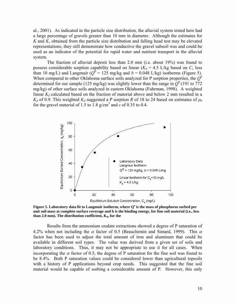
The fraction of alluvial deposit less than 2.0 mm (i.e. about 19%) was found to possess considerable sorption capability based on linear (Kd = 4.5 L/kg based on Ce less than 10 mg/L) and Langmuir (Q0 = 125 mg/kg and b = 0.048 L/kg) isotherms (Figure 5). When compared to other Oklahoma surface soils analyzed for P sorption properties, the Q0 determined for our sample (125 mg/kg) was slightly lower than the range in Q0 (191 to 772 mg/kg) of other surface soils analyzed in eastern Oklahoma (Fuhrman, 1998). A weighted linear Kd calculated based on the fraction of material above and below 2 mm resulted in a Kd of 0.9. This weighted Kd suggested a P sorption R of 18 to 24 based on estimates of ρb for the gravel material of 1.5 to 1.8 g/cm3 and ε of 0.35 to 0.4.

Figure 5. Laboratory data fit to Langmuir isotherm, where Qo is the mass of phosphorus sorbed per unit soil mass at complete surface coverage and b is the binding energy, for fine soil material (i.e., less than 2.0 mm). The distribution coefficient, Kd, for the

Results from the ammonium oxalate extractions showed a degree of P saturation of

4.2% when not including the α factor of 0.5 (Beauchemin and Simard, 1999). This α factor has been used to adjust the total amount of iron and aluminum that could be available in different soil types. The value was derived from a given set of soils and laboratory conditions. Thus, it may not be appropriate to use it for all cases. When incorporating the α factor of 0.5, the degree of P saturation for the fine soil was found to be 8.4%. Both P saturation values could be considered lower than agricultural topsoils with a history of P applications beyond crop needs. This suggested that the fine soil material would be capable of sorbing a considerable amount of P. However, this only

10

pertains to the fine material in the gravel subsoil, which is only about 19% of the entire size fraction.

3.2 Tracer and Phosphorus Injection Experiments

In the first experiment, Rhodamine WT was injected at 100 ppm (Table 1). Samples analyzed from this experiment showed detectable concentrations in all of the piezometers. Concentrations detected in piezometers located 2 to 3 m from the trench (i.e. piezometers A, B, and C) peaked at 36 ppb with peak concentrations occurring approximately 30 min after injection. Detected levels in piezometers located 7 to 8 m from the trench (i.e., piezometers K, L, and M) were generally less than 30 ppb with peak concentrations occurring approximately 50 min after initiation of injection (Figure 6a).

Also, Rhodamine WT concentrations detected in piezometers D, I, and J for the first experiment were much higher than those detected in all other piezometers (Figure 6b). Sample concentrations from these piezometers all exceeded 300 ppb, which was the upper detection limit on the field fluorometer. After dilution in the lab, the concentrations in these wells were found to be close to the injected concentration of 100 ppm. Piezometers D, I, and J were hypothesized to be located in a preferential flow pathway which was more conductive than other subsurface material (Figure 6b).

In the second experiment, Rhodamine WT was injected at approximately 3.0 ppm with the intent of staying within the range of detection for the field fluorometer (Figure 7). Sample analysis showed a pattern similar to the first injection, with detection levels in piezometers D, I, and J approximately equivalent to the injected concentration of 3.0 ppm (Figures 7). However, there was no Rhodamine WT detected in any of the other piezometers. This was hypothesized to be due to the fact that the injected concentration of 3.0 ppm (compared to 100 ppm in the first experiment) was diluted near the detection limit by the time it reached the outer piezometers.

The results from the second Rhodamine WT injection supported the hypothesis that a highly conductive preferential flow pathway existed in the subsoil. The Rhodamine WT concentrations detected in the preferential flow pathway, i.e. Figures 7 (d), (e), and (f) were roughly two orders of magnitude larger than the concentrations detected in the non-preferential flow piezometers, i.e. Figures 7 (b) and (c). This demonstrated the potential for rapid subsurface transport in this alluvial system. These preferential flow pathways in alluvial deposits could represent a direct connectivity with upland nonpoint source pollution sources.

Another trend visible from the Rhodamine WT injections was that samples taken from 10 cm below the water table showed significantly higher concentrations than samples taken 110 cm below the water table for the piezometers considered to be in the preferential flow pathway (Figure 7). These data supported the possibility of layering (i.e., anisotropy) in the subsoil and suggested that the flow is large enough in the preferential flow pathways to inhibit vertical mixing.

Prior to the injection experiments, piezometers were sampled to determine the hydraulic gradient and background P levels. The water levels detected in each piezometer showed minor differences (i.e., less than 1 cm). Therefore, a minimal hydraulic gradient existed which was directed towards the preferential flow pathway. However, during injection, water level readings from two of the piezometers (i.e., D and J) in the

11

preferential flow pathway suggested that water was flowing down the side of the piezometer.

Figure 6. (a) Rhodamine WT concentrations for non-preferential flow piezometers located 2-3 m and 7-8 m from trench during experiment 1. (b) Rhodamine WT concentrations in preferential and non-preferential flow piezometers during experiment 1. Note: Concentrations greater than 300 ppb were above detection limit of field fluorometer.

12

Figure 7. Rhodamine WT concentrations in trench (a) compared to non-preferential flow piezometers (b) and (c) and preferential flow piezometers (d), (e), and (f) during experiment 2.

Background P samples prior to the last injection were grouped according to the

observed piezometer flow response from the Rhodamine WT experiments: (1) preferential flow piezometers versus (2) non-preferential flow piezometers. A statistically significant difference (α = 0.05, p-value = 0.013) was observed between the background P concentration in preferential versus non-preferential flow piezometers (Figure 8). Concentrations of P in the Barren Fork Creek were approximately 1.8 times higher than

13

those observed in the piezometers. The difference between piezometer groupings suggested potential for the preferential flow piezometers to be more directly connected to the stream channel and non-point source loads in the stream.

Figure 8. Box plots of background phosphorus (P) concentration in preferential flow versus non-preferential flow piezometers prior to P injection experiment (i.e., experiment 3). 25th and 75th percentiles = boundary of the box; median = line within the box; 10th and 90th percentiles = whiskers above and below the box.

In the third experiment, KH2PO4 was injected into the trench at a concentration of

100 ppm, as shown in Figure 9. Similar to the Rhodamine WT injections, P concentrations in preferential flow piezometers again mimicked concentrations injected into the trench: Figures 9 (b) and (c). In non-preferential flow piezometers, P was not detected above background concentrations even in piezometers 2 to 3 m from the trench. Although Rhodamine WT was detected in non-preferential flow piezometers 2 to 3 m from the trench at concentrations near 40 ppb, P was not measured above background concentrations (i.e. 40 ppb) in these non-preferential flow piezometers. This result suggested that sorption retarded the movement of P to these non-preferential flow piezometers, and that no significant sorption was observed for piezometers D and J. Two hypotheses were proposed for the lack of sorption that was suggested in piezometers considered to be in the preferential flow pathway: (1) the presence of fewer particles with significant P sorption capability and/or (2) lack of contact time between aqueous and solid phases due to the higher flow velocities. To evaluate the first hypothesis, undisturbed soil cores would be needed from the preferential flow path. However, this was difficult to obtain in the gravel substrate. Therefore, this hypothesis was not evaluated. The second hypothesis was evaluated using flow-cell experiments in the laboratory.

14

Figure 9. Phosphorus concentrations in trench (a) compared to non-preferential flow piezometers (b) and (c) and preferential flow piezometers (d), (e), and (f) during experiment 3.

3.3 Laboratory Flow Experiments Both the contaminant transport and load perspectives suggest that flow velocity had an effect on the sorption capabilities of the system. Figure 10 shows the P concentrations for both velocities plotted versus dimensionless time. Concentrations detected in the outflow solution for the high velocity experiment are approximately 90% of the inflow P

15

concentration after less than 1 min. Therefore, the breakthrough time, tb, for the experiment is less than 1 min. The exact time at which 50% of the sample was detected is not known because the first sample (i.e., at 0.5 min) corresponded to 60% of the inflow concentration. The exponential fit to these data (Figure 10) was used to estimate a tb

* of 2.7, which corresponded to a tb of 0.4 min. For the low flow experiment, the outflow concentration gradually increased with time and reached approximately 75% of the inflow concentration after 8 hrs of injection. The tb determined for the low flow experiment was approximately 155 min, which corresponded to a tb

* of 25.4 (Figure 10).

Figure 10. Phosphorus (P) concentrations detected in outflow (C) versus (a) dimensionless time and (b) mg P added per kg of soil, where Q is the flow rate, Vps is the pore space volume, Cb is the background P concentration released from the soil, Co is the inflow P concentration, and tb

* is the dimensionless breakthrough time.

16

These data suggested that increased P sorption was occurring in the low flow experiment. Specifically, the velocity ratio between the high-flow and low-flow experiments was approximately 36 when using average flow velocities of vh = 46 and vl = 1.3 m/d, respectively. Compared to the ratio of the breakthrough times of approximately 390, additional P sorption was occurring during the low-flow experiment. This could likely be due to the small reaction time between the P and soil surfaces during the high-flow experiment. The flow through experiment data were also analyzed by comparing the total mass of P added to the P concentrations detected in the outflow, as shown in Figure 10b. Variables such as inflow P concentration, mass of P added and mass of soil sample were held constant. The only parameter changed between the two experiments was flow velocity. From Figure 10b, it is noticeable that the outflow P concentrations detected for the low flow experiment were consistently less than the concentrations obtained during the high flow experiment at the same mg of P added per kg of soil. Similar to the contaminant transport analysis, these data also suggest that more P sorption was occurring during low-flow velocity experiments and that flow velocity had an effect on sorption.

This fine (i.e., less than 2.0 mm) material consists of secondary minerals with larger surface areas, such as kaolinite and non-crystalline Al and Fe oxyhydroxides, and is characterized by valence-unsatisfied edge hydroxyl groups. Due to the valency, these edge hydroxyl groups are highly active and account for the majority of P sorption in the material. Although isotherm data on the fine material showed that material had lower sorption properties than other surface soils in Oklahoma, it did suggest that the material was capable of sorbing P. Therefore, the finding that P was sorbing in the low flow experiment is reasonable.

The flow cell experiments suggested that neither variation in fine particle distribution nor P sorption kinetics could be eliminated as factors hypothesized to contribute to the field-observed increased sorption in non-preferential pathways compared to preferential flow pathways. Most likely, a combination of both the presence of fewer fine particles (i.e. soil particles less than 2.0 mm in diameter which possess greater P sorption capability) and the lack of contact time between aqueous and solid phases due to the higher flow velocities in the preferential flow path contributed to the variability in P sorption observations. The Kd estimated from the batch sorption test was 4.5 L/kg. Estimates for Kd obtained from the Ogata and Banks (1961) and Hunt (1978) equations were 11 L/kg and 0.9 L/kg for the low flow and high flow experiments, respectively.

The differences in the Kd values obtained from both the batch sorption isotherm test and the flow-through experiments suggest that nonequilibrium processes were occurring in the system. These processes can be divided into physical and chemical nonequilibrium. Physical non-equilibrium is the result of dissolved P moving into the micropores between the soil particles, resulting in an overestimation of P sorption. Because there was not a large amount of fine clay in the material, the effect of microporosity is likely negligible. Therefore, the differences in the Kd are likely due to a chemical kinetics, meaning that the amount of sorption observed varies due to the time associated with the reaction between dissolved P and the soil surfaces.

17

4.4 Research Implications

This study demonstrated the heterogeneity that existed in the riparian floodplain subsoil can promote significant nutrient transport and confirmed previous research findings by Carlyle and Hill (2001) and McCarty and Angier (2001). Preferential flow pathways may create direct hydraulic connections between nonpoint source loads in the stream and the alluvial gravel subsoil. These direct connections could lead to a transient storage mechanism, where nutrient loads concurrent with large storm events could potentially migrate from the stream into the adjacent floodplain, contaminating the alluvial storage zone. Second, a direct connection may exist between upland sources of P and the streams such that a significant nonpoint source load may not be currently considered in analyzing for the impact of P application and management on such landscapes.

This research has wide reaching implications for how riparian floodplains are managed. Millions of dollars are spent each year to mitigate surface runoff and sediment and nutrient loads. Although these management plans can be effective, this research has shown that subsurface P transport could also be a contributing factor in certain conditions. Because the nutrient load studied here was input directly into the subsurface, the overall subsurface contribution could not be quantified. The next step is determining if similar conditions like this are common and if a direct connection exists between nutrient sources on the surface and the conductive subsurface material.

IV. CONCLUSIONS AND FUTURE WORK

This research demonstrated that subsurface movement of P can be an important transport mechanism, especially in areas such as riparian floodplains with hydraulic conditions conducive to the rapid transport of P. The movement of water and contaminants in riparian floodplains is not homogeneous, and can be impacted by the presence of preferential flow pathways. Concentrations of both Rhodamine WT and P were equivalent at the injection point (i.e., trench) and at preferential flow piezometers located on the southwest side of the trench. However, concentrations of Rhodamine WT and P in non-preferential flow piezometers, some of which were within 2 to 3 m of the trench, did not mimic injected concentrations.

Minimal sorption of P to subsoil material in the preferential flow pathways occurred because of two factors: (1) the presence of fewer fine particles (i.e. soil particles less than 2.0 mm in diameter) and (2) lack of contact time between aqueous and solid phases due to the higher flow velocities. Laboratory flow experiments suggested that the velocity of flow through the subsoil had an effect on P sorption. These findings suggested that high concentrations of P (i.e., concentrations mimicking the injected concentration) detected in the piezometers located in the preferential flow pathway were a result of the greater flow velocity. The velocity, in turn, likely led to a smaller reaction time between the dissolved P and soil surfaces, prohibiting measurable sorption. The lack of P above background concentrations in piezometers outside of the preferential flow pathway may have been a result of the P solution moving much slower through the subsoil and therefore sorbing to the fine material.

18

Because of the quantity of data generated during the field tracer studies, future research is underway to better understand the water quality changes in the alluvial ground water during the injection experiments. Future work is also aimed at investigating the preferential flow pathways in more detail. Electrical resistivity mapping will be used at the field site to attempt to identify and map the preferential flow pathways.

V. ACKNOWLEDGEMENTS This material is based upon work supported by a FY 2007 Oklahoma Water Resources Research Institute and the Oklahoma Water Resources Board grant. The authors acknowledge Dan Butler of the Oklahoma Conservation Commission for providing access to the riparian floodplain property along the Barren Fork Creek.

VI. REFERENCES

Alyamani, M.S., and Z. Sen. 1993. Determination of hydraulic conductivity from complete grain-size distribution curves. Ground Water 31(4):551-555.

Andersen, H.E., and B. Kronvang. 2006. Modifying and evaluating a P index for Denmark. Water Air and Soil Poll. 174(1-4): 341-353.

Beauchemin, S., and R.R. Simard. 1999. Soil phosphorus saturation degree: Review of some indices and their suitability for P management in Quebec, Canada. Can. J. Soil Sci. 79: 615-625.

Carlyle, G.C., and A.R. Hill. 2001. Groundwater phosphate dynamics in a river riparian zone: Effects of hydrologic flow paths, lithology, and redox chemistry. J. Hydrol. 247: 151-168.

Cooper, A.B., C.M Smith, and M.J. Smith. 1995. Effects of riparian set-aside on soil characteristics in an agricultural landscape: Implications for nutrient transport and retention. Agr. Ecosyst. Environ. 55: 61-67.

Daniel, T.C., A.N. Sharpley, and J.L. Lemunyon. 1998. Agricultural phosphorus and eutrophication: A symposium overview. J. Environ. Qual. 27:251-257.

de Jonge, L.W., C. Kjaergaard, and P. Moldrup. 2004. Colloids and Colloid-Facilitated Transport of Contaminants in Soils: An Introduction. Vadose Zone Journal 3: 321-325.

DeSutter, T.M., G.M. Pierzynski, and L.R. Baker. 2006. Flow through and batch methods for determining calcium-magnesium and magnesium-calcium selectivity. Soil Sci. Soc. Am. J. 70:550-554.

Fuhrman, J.K., 1998. Phosphorus sorption and desorption characteristics of Oklahoma soils. M.S. Thesis, Oklahoma State University, Stillwater, OK.

Heathwaite, L., P. Haygarth, R. Matthews, N. Preedy, and P. Butler. 2005. Evaluating colloidal phosphorus delivery to surface waters from diffuse agricultural sources. J. Environ. Qual. 34 (1): 287-298.

Hively, W.D., P. Gerard-Marchant, and T.S. Steenhuis. 2006. Distributed hydrological modeling of total dissolved phosphorus transport in an agricultural landscape II. Dissolved phosphorus transport. Hydrology and Earth System Sciences 10(2): 263-276.

19

20

Hunt, B. 1978. Dispersive sources in uniform ground-water flow. J. Hydraul. Eng.-ASCE 104(HY1): 75-85.

Ilg, K., and M. Kaupenjohann. 2005. Colloidal and dissolved phosphorus in sandy soils as affected by phosphorus saturation. J. Environ. Qual. 34: 926-935.

Iyengar, S.S., L.W. Zelazny, and D.C. Martens. 1981. Effect of photolytic oxalate treatments on soil hydroxyl interlayered vermiculites. Clay. Clay. Miner. 29: 429-434.

Kleinman, P.J.A., B.A. Needelman, A.N. Sharpley, and R.W. McDowell. 2004. Using soil phosphorus profile data to assess phosphorus leaching potential in manured soils. Soil Sci. Soc. Am. J. 67 (1): 215-224.

Landon, M.K., D.L. Rus, and F.E. Harvey. 2001. Comparison of instream methods for measuring hydraulic conductivity in sandy streambeds. Ground Water 39(6): 870-885.

McCarty, G., and J. Angier. 2001. Impact of preferential flow pathways on ability of riparian wetlands to mitigate agricultural pollution. In Preferential Flow: Water Movement and Chemical Transport in the Environment, Proc. 2nd International Symposium. (3-5 January 2001, Honolulu, Hawaii. USA), eds David Bosch and Kevin King., St. Joseph, Michigan: American Society of Agricultural Engineers. pp 53-56.

McKeague, J., and J.H. Day. 1966. Diothionite and oxalate-extractable Fe and Al as aids in differentiating various classes of soils. Can. J. Soil Sci. 46: 13-22.

Murphy, J., and J.R. Riley. 1962. A modified single solution method for the determination of phosphate in natural waters. Anal. Chim. Acta 27: 31-36.

Nelson, N.O., J.E. Parsons, and R.L. Mikkelson. 2005. Field-scale evaluation of phosphorus leaching in acid sandy soils receiving swine waste. J. Environ. Qual. 34(6): 2024-2035.

Ogata, A., and R.B. Banks. 1961. A solution of the differential equation of longitudinal dispersion in porous media. U.S. Geological Survey Prof. Paper 411-A.

Osborne, L.L., and D.A. Kovacic. 1993. Riparian vegetated buffer strips in water-quality restoration and stream management. Freshwater Biol. 29(2): 243-258.

Owens, L.B., and M.J. Shipitalo. 2006. Surface and subsurface phosphorus losses from fertilized pasture systems in Ohio. J. Environ. Qual. 35: 1101-1109.

Polyakov, V., A. Fares, and M. H. Ryder. 2005. Precision riparian buffers for the control of nonpoint source pollutant loading into surface water: A review. Environ. Rev. 13: 129-144.

Pote, D.H., T.C. Daniel, A.N. Sharpley, P.A. Moore, Jr., D.R. Edwards, and D.J. Nichols. 1996. Relating extractable soil phosphorus to phosphorus losses in runoff. Soil Sci. Soc. Am. J. 60: 855-859.

Sauer, T.J., and S.D. Logsdon. 2002. Hydraulic and physical properties of stony soils in a small watershed. Soil Sci. Soc. Am. J. 66:1947–1956.

Turner, B.L., and P.M. Haygarth. 2000. Phosphorus forms and concentrations in leachate under four grassland soil types. Soil Sci. Soc. Am. J. 64 (3): 1090-1099.

Vanek, V. 1993. Transport of groundwater-borne phosphorus to Lake Bysjon, South Sweden. Hydrobiologia 251(1-3): 211-216.

Determination of Fracture Density in the Arbuckle−SimpsonAquifer from Ground Penetrating Radar (GPR) andResistivity Data

Basic Information

Title:Determination of Fracture Density in the Arbuckle−Simpson Aquifer fromGround Penetrating Radar (GPR) and Resistivity Data

Project Number: 2007OK80B

Start Date: 3/1/2007

End Date: 2/28/2008

Funding Source:104B

Congressional District:2, 3 &4

Research Category:Ground−water Flow and Transport

Focus Category:Water Supply, Hydrology, Models

Descriptors:Arbuckle−Simpson Aquifer, Ground Penetrating Radar, Fracture Density,Rock Resistivity

Principal Investigators: Ibrahim Cemen, Todd Halihan, Roger Young

Publication

Halihan, T., 2008. Evaluating Groundwater−Surface Water Interactions Using ERI in theArbuckle−Simpson Aquifer, GSA South−Central Sectional Meeting, Hot Springs, AK, April 2008,Geological Society of America Abstracts with Programs, Vol. 40, No. 3, p. 30.

1.

Determination of Fracture Density in the Arbuckle−Simpson Aquifer from Ground Penetrating Radar (GPR) and Resistivity Data1

INTERIM TECHNICAL REPORT Determination of Fracture Density in the Arbuckle-Simpson Aquifer from Ground

Penetrating Radar (GPR) and Resistivity Data Principal Investigators: Ibrahim Cemen and Todd Halihan, Boone Pickens School of Geology, Oklahoma State

University Roger A. Young, Conoco/Phillips School of Geology, University of Oklahoma Problem and Research Objectives:

The ground water resources of Oklahoma are vital to the economic well being of the state. In order to properly manage these resources, an understanding of the discharge and recharge of aquifers is necessary. Fractures in aquifer rocks affect the flow of water. Therefore, numerical modeling of the fluid flow requires an understanding of the nature of fractures that have a great influence on the discharge and recharge mechanisms.

The Arbuckle-Simpson aquifer of southern Oklahoma is a major source of drinking water for communities in the south-central part of the state. In outcrops, the carbonate units of the Arbuckle-Simpson are highly fractured. The basement rocks underlying the Arbuckle-Simpson aquifer are also highly fractured in outcrop. For example, the granites exposed in the Devil’s Den area near Tishomingo, Oklahoma exhibit extensive fracturing and faulting. The characterization of fractures in the basement is also important for ground water modeling work currently underway at both the Oklahoma Water Resources Board (OWRB) and the United States Geological Survey (USGS). Therefore, mapping fracture density from geophysical data such as Ground Penetrating Radar (GPR) and Resistivity would provide timely information for these modeling studies

Methodology:

We have identified two survey sites to carry out the work proposed here. We have authorization to access both of these sites. The first site is Arbuckle-Simpson Ranch in southern Oklahoma. Dolomite of the Lower Arbuckle Group in this area is extensively fractured in outcrops in this area. The second site is in the Devil’s Den area of Tishomingo, Oklahoma where Precambrian age granite is exposed at the surface. The granite is highly fractured in places and is an excellent site for our work because of the absence of conductive overburden which limits the depth of penetration of GPR signal and electrical current. The granitic environment does present a challenge for drilling holes to plant electrodes in the ground for electrical resistivity work.

The direct current resistivity method is a commonly used surface geophysical technique to map the resistivity (inverse of conductivity) of the shallow subsurface. The variations in observed resistivity depend on many factors including the rock matrix, presence of fluids, salinity, and faults and fractures (Figure 1). Figure 2 shows the azimuthal variation in resistivity in the presence of fractures. In this case, the data was acquired with the Wenner configuration of current and voltage electrodes. Phase 2 of our work will test the feasibility of using the Wenner and other electrode configurations for determining the fracture orientation and density. We will also assess the feasibility of conducting 3-D resistivity surveys during Phase 2 of the project.

The GPR data will be acquired with the equipment owned by Oklahoma State University and the University of Oklahoma. A PulseEkko 100 system is owned by Oklahoma State University. This is a 1000 Volt system with antenna frequency of 200 MHz. The University of of Oklahoma also owns a 450 MHz transmitter-receiver PulseEkko GPR system which should be capable of providing high resolution data. Data processing will be done by a variety of software packages (Win_Ekko, Ekko_view Deluxe, SPW) owned by both Oklahoma State University and the University of Oklahoma. We also have state-of-the-art visualization facilities at Oklahoma State University which should aid in the interpretation of the 3-D GPR volumes. The University of Oklahoma also has a suite of energy industry wave-field processing packages including both licensed software (such as the Kingdom and Hampson-Russell software) and proprietary software for attribute analysis. .The experience of the PIs in attribute analysis of time-series data would be important for extracting useful information from the GPR data for fracture characterization of the Arbuckle-Simpson aquifer. Other relevant software available to this project includes numerous interpretation packages available to OSU and OU. There is also the capability of spectral decomposition analysis at OU for enhanced interpretation of GPR data.

Figure 1: Plot of reflection coefficient as a function of horizontal layer thickness (fracture) within a rock matrix with dielectric properties of Byron Dolomite for 200 MHz GPR signal [From Tsoflias et al., 2001]

Figure 2: Azimuthal dependence of resistivity in the presence of fractures. The long axis of the ellipse drawn around the center point shows the direction of fractures to be approximately N79E. (From Cohen and Rudman, 1995) The resistivity data will be acquired with AGI’s Super Sting multi-channel imaging

system owned by Oklahoma State University. The resistivity system has been used extensively by Todd Halihan and his students to map fractures at several sites in Oklahoma in support of projects at the Oklahoma Water Resources Board. In addition to the field equipment, the Oklahoma State University owns state-of-the-art resistivity inversion and other software tools to process the data.

Principal Findings and Significance: The ERI data is being intergrated with shallow borings, GPR, and seismic data to understand how the methods can be used in conjunction to understand the fracturing of the aquifer.

The ERI data provided good control over the shallow weathering of the aquifer and faulting that occurred in the study sites.

Information Transfer Program Introduction

Activities for the efficient transfer and retrieval of information are an important part of the OWRRI programmandate. The Institute maintains a website on the Internet (http://environ.okstate.edu/owrri) that providesinformation on the OWRRI and supported research, grant opportunities and deadlines, and upcoming events.Abstracts of technical reports and other publications generated by OWRRI projects are updated regularly andare accessible on the website.

The OWRRI produces a quarterly newsletter entitled "The Aquahoman" to disseminate research results andprovide information on upcoming events and grant competitions.

The OWRRI sponsors a water research symposium in the fall of each year at which OWRRI−sponsoredprojects are presented, along with many others. This year's water research symposium was held, for the firsttime, in conjunction with the annual Governor's Water Conference. This significantly increased attendancefrom approximately 130 participants to over 400.

In addition, to keep state water professionals apprised of our work, updates on current−year projects arepresented at the OWRRI's Water Research Advisory Board, which consists of representatives from 24 stateand federal water agencies, as well as non−government organizations. The WRAB is a unique gathering of theState's water agencies, Native American tribes, and water−interested NGOs. As such it has not only become apopular meeting for its members (who report that they have no other opportunity to gather with all of the otherstate's water organizations and agencies), but has also become a popular venue for seeking advice on waterrelated−topics.

Due to the amount of work taken on by the Board, the WRAB now meets once each winter and summer. Inaddition to determining funding priorities for OWRRI's annual research competition and assisting with theselection of funded projects, the WRAB has begun to play a vital role in the state's water planning efforts byproviding feedback and advice regarding the OWRRI's efforts to gather public input about policyrecommendations.

Information Transfer Program Introduction 1

Student Support

Student Support

CategorySection 104 Base

GrantSection 104 NCGP

AwardNIWR−USGS

InternshipSupplemental

AwardsTotal

Undergraduate 3 0 0 0 3

Masters 6 0 0 0 6

Ph.D. 2 0 0 0 2

Post−Doc. 0 0 0 0 0

Total 11 0 0 0 11

Student Support 1

Notable Awards and Achievements

In 2007, OWRRI began its effort to gather public input on policy suggestions for the Oklahoma's update ofthe comprehensive water plan. The OWRRI is under contract with Oklahoma Water Resources Board(OWRB) for this effort and has designed a novel approach for gathering public input. Utilizing the values ofthe public as well as the best expertise available, the goal of this four and a half year process is to develop aplan that enjoys broad support and is well informed. The effort will involve approximately 70 public meetingsacross the state to gather, consolidate, and prioritize citizens' concerns, and then, develop policyrecommendations regarding state water issues.

The first 18 months have been very successful, consisting of 42 Local Input Meetings held throughoutOklahoma in 2007. In this phase, approximately 2500 people participated and made over 2400 comments − byfar the most public involvement in a state water plan in Oklahoma and perhaps the nation.

As part of this planning effort, the OWRB has joined the OWRRI in funding research to address the state'swater planning needs by providing a match to the money granted by the US Geological Survey.

Notable Awards and Achievements 1