ol. 60, no. 1 - uc davis department of economics · ol. 60, no. 1 the economic history review ......
TRANSCRIPT
Vol. 60, N
o. 1T
HE
EC
ON
OM
IC H
ISTO
RY
RE
VIE
WFebruary 2007
CONTENTS
ARTICLESGLEN O’HARA
Towards a new Bradshaw? Economic statistics and the British state in the 1950s and 1960s
E. A. WRIGLEYEnglish county populations in the later eighteenth century
GRAHAM BROWNLOWThe causes and consequences of rent-seeking in Northern Ireland,
1945–72
GREGORY CLARKThe long march of history: Farm wages, population, and economic
growth, England 1209–1869
REVIEW OF PERIODICAL LITERATUREDAVID PRATT, P. R. SCHOFIELD, HENRY FRENCH, PETER KIRBY,
MARK FREEMAN AND JULIAN GREAVES, AND HUGH PEMBERTON
BOOK REVIEWS
This journal is available online at BlackwellSynergy. Visit www.blackwell-synergy.com tosearch the articles and register for table ofcontents e-mail alerts.
VOLUME 60, NO. 1 FEBRUARY 2007
0013-0117(200702)60:1;1-I

Economic History Review
, 60, 1 (2007), pp. 97–135
© Economic History Society 2006. Published by Blackwell Publishing, 9600 Garsington Road, Oxford OX4 2DQ, UK and 350 MainStreet, Malden, MA 02148, USA.
Blackwell Publishing Ltd.Oxford, UK and Malden, USAEHRThe Economic History Review0013-0117Economic History Society 20062007
60
197135Articles
THE LONG MARCH OF HISTORYGREGORY CLARK
The long march of history: Farm wages, population, and economic
growth, England 1209–1869
1
By GREGORY CLARK
SUMMARY
The article forms three series for English farm workers from 1209–1869:nominal day wages, the implied marginal product of a day of farm labour,and the purchasing power of a day’s wage in terms of farm workers’ consump-tion. These series suggest that labour productivity in English agriculture wasalready high in the middle ages. Furthermore, they fit well with one methodof estimating medieval population that suggests a peak English population
c.
1300 of nearly 6 million. Lastly, they imply that both agricultural technologyand the general efficiency of the economy were static from 1250 till 1600.Economic changes were in these years entirely a product of demographicshifts. From 1600 to 1800, technological advance in agriculture provided analternative source of dynamism in the English economy.
he wage and price history of pre-industrial England is uniquely welldocumented. England achieved substantial political stability by 1066.
There was little of the internal strife that proved so destructive of documen-tary history in other countries. In addition, England’s island position andrelative military success protected it from foreign invasion, except for thedepredations of the Scots along the northern border. England further wit-nessed the early development of markets and monetary exchange. In par-ticular, though surviving reports of privately paid wages exist only from1209, the payment of money wages to workers was clearly already wellestablished by that date. A large number of documents with such wages andprices survive from then on in the records of churches, monasteries, col-leges, charities, and government.
These documents have been the basis of many studies of pre-industrialwages and prices. But comparatively few of these studies have focused onthe wages of the majority of workers in England before 1800, those inagriculture. And none of the farm wage studies give a consistent measure
1
The research in this paper was funded by National Science Foundation (NSF) grants SES 91-22191and SES 02-41376. I thank Joyce Burnette and John Munro for their great generosity in sharing dataon wages they assembled from manuscript sources. John Munro also shared with me his entries ofthreshing payments and day wages for the Winchester estates from the Beveridge Archive at LSE.Without their gifts this article would be considerably diminished. Bruce Campbell made extensiveconstructive criticisms.
T
98
GREGORY CLARK
© Economic History Society 2006
Economic History Review
, 60, 1 (2007)
of both nominal and real wages over the long pre-industrial era.
2
It isimpossible to even get an estimate of real farm day wages in 1300 comparedto 1800 using these sources without having to chain together five differentsources.
Assembling the available evidence on farm wages, including both newmanuscript material and unpublished material from the archives of LordBeveridge and David Farmer, this article constructs a consistent series forthe estimated day wages of male farm labourers from 1209 to 1869. Divid-ing nominal wages by an index of the prices of farm output, the article alsoestimates the marginal product of labour (MPL) in agriculture.
3
Thisderivation assumes that cultivators hired labour up to the point where theday wage equalled the value of the extra output gained from an extra dayof labour input. However, the article shows that cultivators did respond tothe cost of labour when making decisions about how much to employ evenfor the medieval period. The article further estimates the purchasing powerof the day wage for the goods bought by farm labourers, which is of coursetheir real wage. The nominal and real wages by year are reported in theappendix.
The second part of the article explores the implications of these series forEnglish economic history. The MPL estimate can be used to get an ideaof output per worker in agriculture over time. They suggest some gains inoutput per worker between 1300 and 1800, but much less than manyauthors estimate.
4
They also suggest that
c.
1450, output per worker inagriculture in England was as high as in 1850.
But the huge swings evident in the MPL suggest that output per workeralone is a poor guide to agricultural efficiency. To say anything, we need toknow the number of workers in agriculture, or failing that overall popula-tion. The article also estimates a decadal series for population in Englandfrom 1200 to 1530. I show the validity of this series by correlating it withthe MPL from 1250–1530. The close match argues strongly in favour ofthis series, and for the conclusion that agricultural efficiency remainedunchanged from 1250 to 1530. With the modest assumption of no efficiencyadvance between the 1520s and 1540s it is also possible to fix the impliedlevel of population for the years before 1530. The suggested peak medievalpopulation is 6 million, at the high end of estimates in the literatureand in line with the views of Postan and, more recently, Richard Smith.
5
The MPL series rejects the more recent revisionism of Bruce Campbelland Ian Blanchard, which suggests a maximum medieval population of
2
Beveridge, ‘Wages’, gives piece rates and day wages by decade for farm workers on the Winchesterestates from 1209–1453, but no cost of living measures. Farmer, ‘Prices and wages’, and ‘Prices andwages, 1350–1500’, gives annual piece rates only for 1209–1474, and a limited cost of living measure.Bowden, ‘Statistical appendix’, gives decadal estimates of day wages from 1450 to 1750, sometimesdrawn only from Oxford and Cambridge, but again with very imperfect cost-of-living measures.
3
The price index is from Clark, ‘Price history’.
4
See, for example, Wrigley, ‘Transition’.
5
Smith, ‘Human resources’, pp. 189–91, Smith, ‘Demographic developments’.
THE LONG MARCH OF HISTORY
99
© Economic History Society 2006
Economic History Review
, 60, 1 (2007)
4–4.5 million.
6
If the index were set to the level of 4 million in 1300, assuggested by Campbell, then it would generate implausible implications forthe years 1500–40. The implied level of population in the 1520s would be1.6 million, which would have to grow to 3 million by the 1540s: a rate of3 per cent per year. At the same time as this unprecedented populationgrowth, agricultural productivity would have to advance substantially justin these years to keep the MPL from falling sharply. A new populationestimate that explicitly incorporates the evidence of the MPL is proposedby decade for the years 1250–1540.
Lastly, the article shows that the MPL and real wage estimates, combinedwith what we know about population, suggest stasis both in agriculturaltechnology and in the general efficiency of the economy from 1250 to atleast 1600. This was followed by a period of efficiency growth that precededthe Industrial Revolution. The only other period before 1800 where theeconomy potentially experienced an efficiency advance is in the earlythirteenth century. The real wage evidence is consistent with the Malthusianmodel of the determination of incomes and population levels for Englandall the way from 1200 to 1800. Living standards were determined by fertilityand mortality rates, and population adjusted to these living standards. Thereis no sign of any secular trend towards higher living standards in the pre-industrial era.
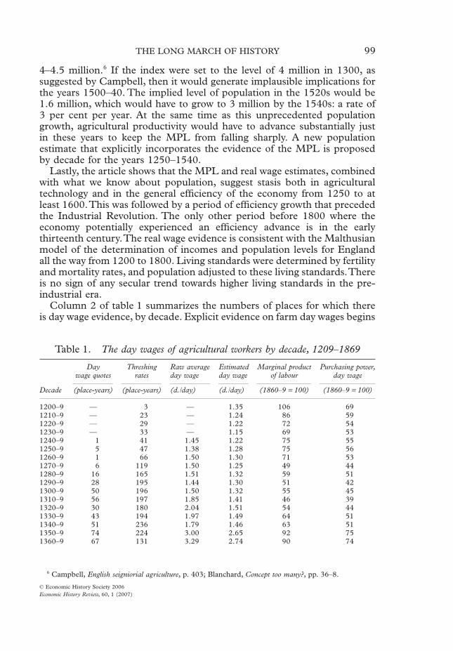
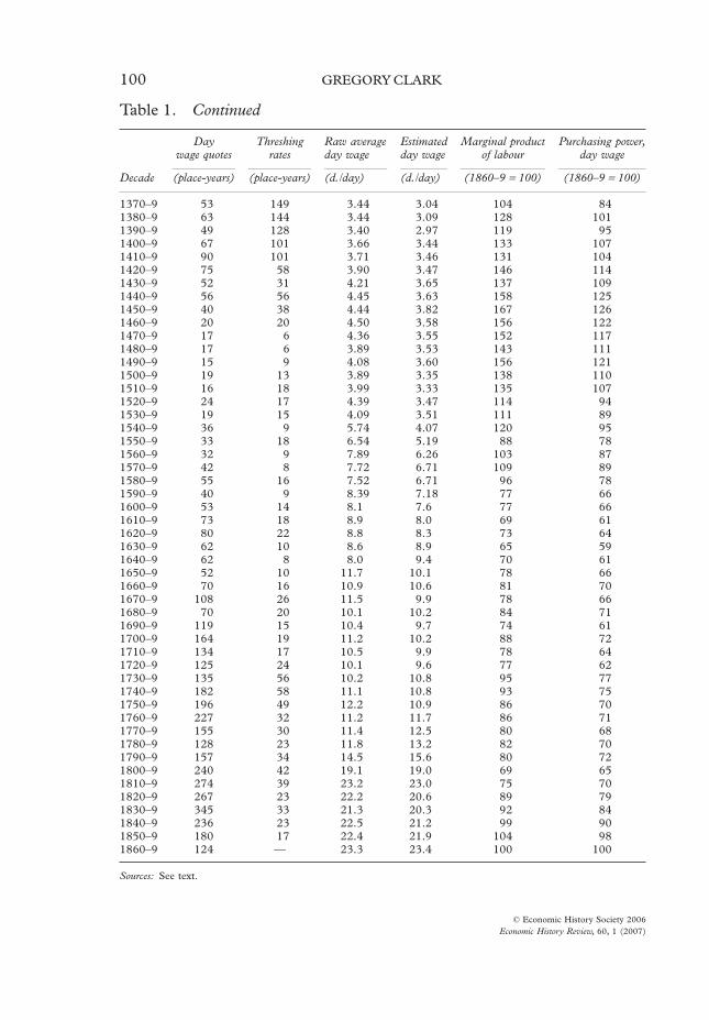
Column 2 of table 1 summarizes the numbers of places for which thereis day wage evidence, by decade. Explicit evidence on farm day wages begins
6
Campbell,
English seigniorial agriculture
, p. 403; Blanchard,
Concept too many?
, pp. 36–8.
Table 1.
The day wages of agricultural workers by decade, 1209–1869
Decade
Daywage quotes
Threshingrates
Raw averageday wage
Estimatedday wage
Marginal productof labour
Purchasing power,day wage
(place-years) (place-years) (d./day) (d./day) (1860–9
=
100) (1860–9
=
100)
1200–9 — 3 — 1.35 106 691210–9 — 23 — 1.24 86 591220–9 — 29 — 1.22 72 541230–9 — 33 — 1.15 69 531240–9 1 41 1.45 1.22 75 551250–9 5 47 1.38 1.28 75 561260–9 1 66 1.50 1.30 71 531270–9 6 119 1.50 1.25 49 441280–9 16 165 1.51 1.32 59 511290–9 28 195 1.44 1.30 51 421300–9 50 196 1.50 1.32 55 451310–9 56 197 1.85 1.41 46 391320–9 30 180 2.04 1.51 54 441330–9 43 194 1.97 1.49 64 511340–9 51 236 1.79 1.46 63 511350–9 74 224 3.00 2.65 92 751360–9 67 131 3.29 2.74 90 74
Sources:
See text.
100
GREGORY CLARK
© Economic History Society 2006
Economic History Review
, 60, 1 (2007)
1370–9 53 149 3.44 3.04 104 841380–9 63 144 3.44 3.09 128 1011390–9 49 128 3.40 2.97 119 951400–9 67 101 3.66 3.44 133 1071410–9 90 101 3.71 3.46 131 1041420–9 75 58 3.90 3.47 146 1141430–9 52 31 4.21 3.65 137 1091440–9 56 56 4.45 3.63 158 1251450–9 40 38 4.44 3.82 167 1261460–9 20 20 4.50 3.58 156 1221470–9 17 6 4.36 3.55 152 1171480–9 17 6 3.89 3.53 143 1111490–9 15 9 4.08 3.60 156 1211500–9 19 13 3.89 3.35 138 1101510–9 16 18 3.99 3.33 135 1071520–9 24 17 4.39 3.47 114 941530–9 19 15 4.09 3.51 111 891540–9 36 9 5.74 4.07 120 951550–9 33 18 6.54 5.19 88 781560–9 32 9 7.89 6.26 103 871570–9 42 8 7.72 6.71 109 891580–9 55 16 7.52 6.71 96 781590–9 40 9 8.39 7.18 77 661600–9 53 14 8.1 7.6 77 661610–9 73 18 8.9 8.0 69 611620–9 80 22 8.8 8.3 73 641630–9 62 10 8.6 8.9 65 591640–9 62 8 8.0 9.4 70 611650–9 52 10 11.7 10.1 78 661660–9 70 16 10.9 10.6 81 701670–9 108 26 11.5 9.9 78 661680–9 70 20 10.1 10.2 84 711690–9 119 15 10.4 9.7 74 611700–9 164 19 11.2 10.2 88 721710–9 134 17 10.5 9.9 78 641720–9 125 24 10.1 9.6 77 621730–9 135 56 10.2 10.8 95 771740–9 182 58 11.1 10.8 93 751750–9 196 49 12.2 10.9 86 701760–9 227 32 11.2 11.7 86 711770–9 155 30 11.4 12.5 80 681780–9 128 23 11.8 13.2 82 701790–9 157 34 14.5 15.6 80 721800–9 240 42 19.1 19.0 69 651810–9 274 39 23.2 23.0 75 701820–9 267 23 22.2 20.6 89 791830–9 345 33 21.3 20.3 92 841840–9 236 23 22.5 21.2 99 901850–9 180 17 22.4 21.9 104 981860–9 124 — 23.3 23.4 100 100
Decade
Daywage quotes
Threshingrates
Raw averageday wage
Estimatedday wage
Marginal productof labour
Purchasing power,day wage
(place-years) (place-years) (d./day) (d./day) (1860–9
=
100) (1860–9
=
100)
Sources:
See text.
Table 1.
Continued
THE LONG MARCH OF HISTORY
101
© Economic History Society 2006
Economic History Review
, 60, 1 (2007)
only in the 1240s, and then on a limited basis. The evidence is also thin for1460–1540. To supplement the day wage evidence, payments per bushel forthreshing grain were used. Such piece-rate payments were more abundantfor the middle ages than day wages. Column 3 of table 1 shows the numbersof places contributing information on threshing payments by decade. Suchthreshing payments are available back to 1209 on some Winchester manors.In the years 1460 to 1540 the threshing evidence, though limited, helps fillout the scant day wage evidence.
To combine these two sources into a day wage estimate, a regressioncombining day wages and threshing piece rate payments is employed. Handthreshing as a task did not change technologically from 1209 to 1850.However, at times when day wages were high relative to grain prices, thethreshing payment per bushel fell relative to the day wage. Assuming pieceand day workers earned the same wage per day, the implied number ofbushels threshed per day thus changed over time. The regression accom-modates this by using the threshing payments only to fill in the wage series,but not determine its long-run level. The only exception is the years before1349, when it is assumed that threshing rates were constant since real wagesvaried by more modest amounts in this interval. Wages were sometimesquoted by season so allowance was made for seasonal differences in wages.The unit of observation was the average payment in a given season of agiven year and place for a particular type of work. Treated this way the35,000 records in the wages database reduced to 19,417 observations.Table 2 shows the composition of the various types of observation in thissample. Direct day wage quotes provide less than half the observations.
The average day wage varied widely by location. In the medieval period,for example, day wages on the Westminster manors of Eybury, Hyde, andKnightsbridge near London were about 28 per cent higher than averagewages on a selection of the Winchester manors. In years where there are
Table 2.
The types of data used in estimating day wages
Type of wage quote Numbers of observations
Day wage: 8,511Winter (October–March) 2,074Summer (April–September) 1,608Harvest 726Hay 616Season unknown 3,675
Threshing payment: 10,521Wheat 2,447Rye 545Barley 2,262Oats 2,024Peas 967Other 2,661
Source:
Wage payment database.

102
GREGORY CLARK
© Economic History Society 2006
Economic History Review
, 60, 1 (2007)
few wage observations sampling error can thus be significant. There werealso regional differences in wage trends, with the north in particular showingmore wage growth over time. In the regression, fixed effects for location areincluded to control for persistently higher wage levels in areas near towns.Time trends for the north, midland, and southwest regions were includedto control for different regional wage trends.
The appendix reports the exact specification of the regression, and thevalues of the major control variables estimated. A comparison of the esti-mated level of this wage series with the broad cross sections of wagesavailable in the years 1767–70 (from Arthur Young), 1832 (from the PoorLaw Report), and 1849–50 and 1859–60 (from the
Gardeners’ Chronicle
and
Agricultural Gazette
) reported in table 3 suggests that it averages 4.7 per centbelow the national farm wage. The reason may be that the benchmarkaverages include allowances for the money value of beer given to workersat work, which the data in this sample generally does not include. The finalnominal wage series was adjusted upwards in all years by 4.9 per cent to fitthese benchmarks. Once that is done the adjusted series fits the benchmarkswell, as table 3 shows. Appendix table A2 records the resulting estimatednational day wage outside hay and harvest by year.
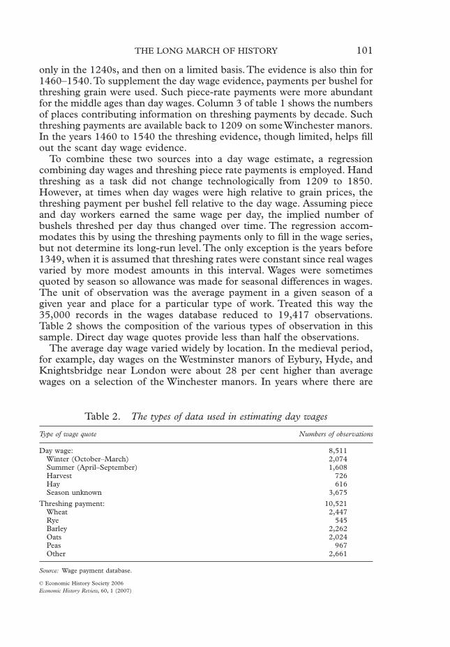
Figure 1 shows the raw average day wage by decade, not controlling forplace or location, compared to the estimated national wage derived fromthe regression. It is noticeable that the national nominal day wage estimatedhere is typically 80–85 per cent of the raw averages before 1700. The sourceof this deviation is twofold. Earlier wages tended to be drawn more heavilyfrom high-wage farms near urbanized locations, such as Hyde, Knights-bridge, and Eybury near London. In contrast, after 1760 the wages comemainly from very rural locations. Before 1700 the wages were drawnheavily from the south, which was then the high wage location. Thus before1700, 59 per cent of observations are from the south east, in contrastto 3 per cent from the north. The regional trends in the regression equationcorrect for this under-representation. Figure 1 also shows that both Bever-idge’s estimate of nominal day wages on a sample of the Winchester estatesbefore 1453 and Bowden’s estimates of day wages from 1450 to 1750 aregenerally too high, though by variable amounts.
Table 3.
Comparison of wages with benchmark estimates
Period Source LocationsAverage day wage
outside harvestWage fromregression
Final wageestimate
1767–70 Young 140 12.0 11.3 11.81832 Poor Law Report 931 20.9 19.9 20.91850
Gardeners’ Chronicle
123 18.6 18.0 18.91860
Gardeners’ Chronicle
70 22.0 21.0 22.0
Source:
See Clark, ‘Farm wages’ for sources on the benchmark estimates.
THE LONG MARCH OF HISTORY
103
© Economic History Society 2006
Economic History Review
, 60, 1 (2007)
One measure of whether the estimation procedure improves the estimateof wages is to compare the variance of the raw wage averages with that ofthe estimated day wage in periods of little trend in nominal wages. For theyears 1250 to 1349 the coefficient of variation of the raw average wages is0.23, and of the estimated day wages 0.08, less than half as large. For 1350to 1549 the coefficient of variation of the raw wage level is 0.19, and forthe estimated wage 0.12. Thus for these early years the estimation procedureremoves a lot of noise from the yearly wage estimates.
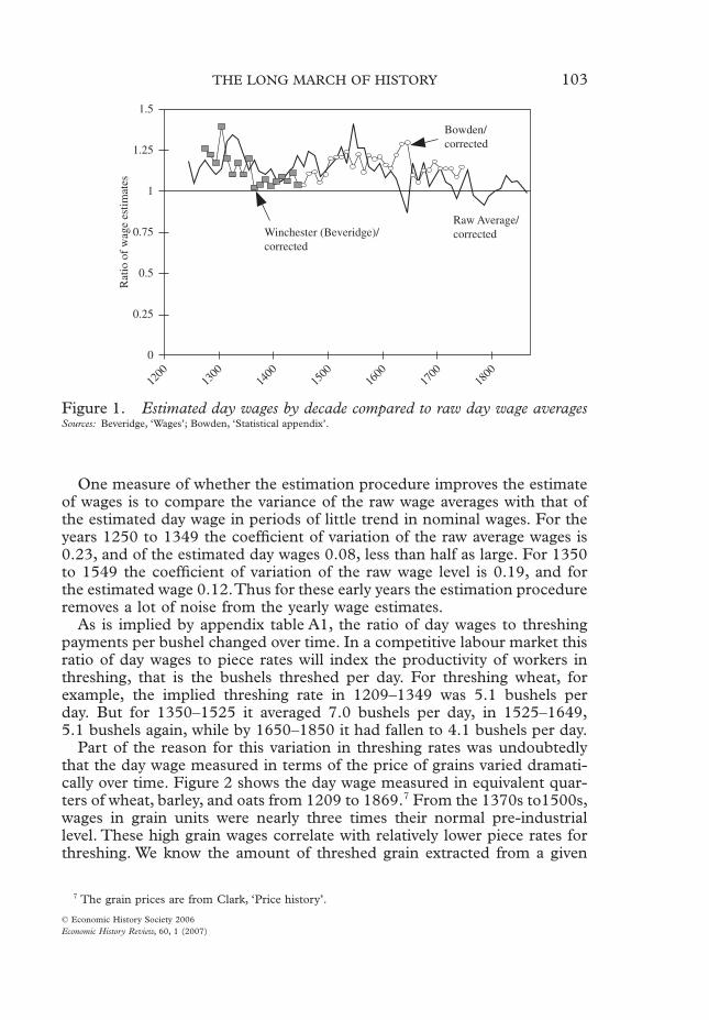
As is implied by appendix table A1, the ratio of day wages to threshingpayments per bushel changed over time. In a competitive labour market thisratio of day wages to piece rates will index the productivity of workers inthreshing, that is the bushels threshed per day. For threshing wheat, forexample, the implied threshing rate in 1209–1349 was 5.1 bushels perday. But for 1350–1525 it averaged 7.0 bushels per day, in 1525–1649,5.1 bushels again, while by 1650–1850 it had fallen to 4.1 bushels per day.
Part of the reason for this variation in threshing rates was undoubtedlythat the day wage measured in terms of the price of grains varied dramati-cally over time. Figure 2 shows the day wage measured in equivalent quar-ters of wheat, barley, and oats from 1209 to 1869.
7
From the 1370s to1500s,wages in grain units were nearly three times their normal pre-industriallevel. These high grain wages correlate with relatively lower piece rates forthreshing. We know the amount of threshed grain extracted from a given
7
The grain prices are from Clark, ‘Price history’.
Figure 1.
Estimated day wages by decade compared to raw day wage averages
Sources:
Beveridge, ‘Wages’; Bowden, ‘Statistical appendix’.
1.5
1.25
1
0.75
Rat
io o
f w
age
estim
ates
0.5
Winchester (Beveridge)/corrected
Raw Average/corrected
Bowden/corrected
0.25
0
1200
1300
1400
1500
1600
1700
1800

104
GREGORY CLARK
© Economic History Society 2006
Economic History Review
, 60, 1 (2007)
quantity of grain in the sheaf increases with longer threshing. When wageswere low it would be profitable to thresh each sheaf longer and extract moreof the grain. But even controlling for this there is still a downwards seculartrend in the implied numbers of bushels threshed controlling for the grainwage. The reason for this secular decline in threshing rates is unclear.Perhaps types of grain were developed which had less easily shed seed thatrequired more threshing to extract from the straw.
8
One implication of the changing threshing rates is that the threshingpayments reported by Lord Beveridge and David Farmer as an index offarm wages in the years 1209–1474 do not serve as a reliable proxy for daywage rates.
9
Threshing payments increased much less between 1350 and1400 than actual measures of day wages. For the years before 1270, whenI mainly rely on threshing payments to estimate day wages, we thus needto make an assumption about what the ratio was in this period. It is assumedfor these years that it was the same as that of 1270–1349. The resultingestimates of real wages suggest they were not too much higher before 1275than they were for 1275–49, and we see above that grain wages are animportant predictor of threshing rates, so this assumption is consistent withthe resulting wage estimates.
8
The gain from this would be less wastage of grain through early dropping of seed in the field.
9
Beveridge, ‘Wages’; Farmer, ‘Prices and wages’.
Figure 2.
Real day wages measured in terms of grain (wheat, barley, oats)
Note:
The wage in grain units is indexed at 100 on average for the years 1860–9.
Source:
The grain prices are from Clark, ‘Price history’.
250
200
150
100
50
0
Farm
wag
e in
bus
hels
of
grai
n
1200
1300
1400
1500
1600
1700
1800

THE LONG MARCH OF HISTORY
105
© Economic History Society 2006
Economic History Review
, 60, 1 (2007)
Having derived nominal wages there are two types of ‘real’ wage that canbe calculated. The first is the cost of labour to the farmer relative to thegoods being produced on the farm. This does not matter to the labourer,but in a labour market where employers seek to maximize profits it willmeasure the marginal product of farm labour (MPL), the amount of extraoutput each day of labour produced on the margin. In such a case
(1)
So
(2)
where
w
is the nominal wage and
p
the price of farm output.
10
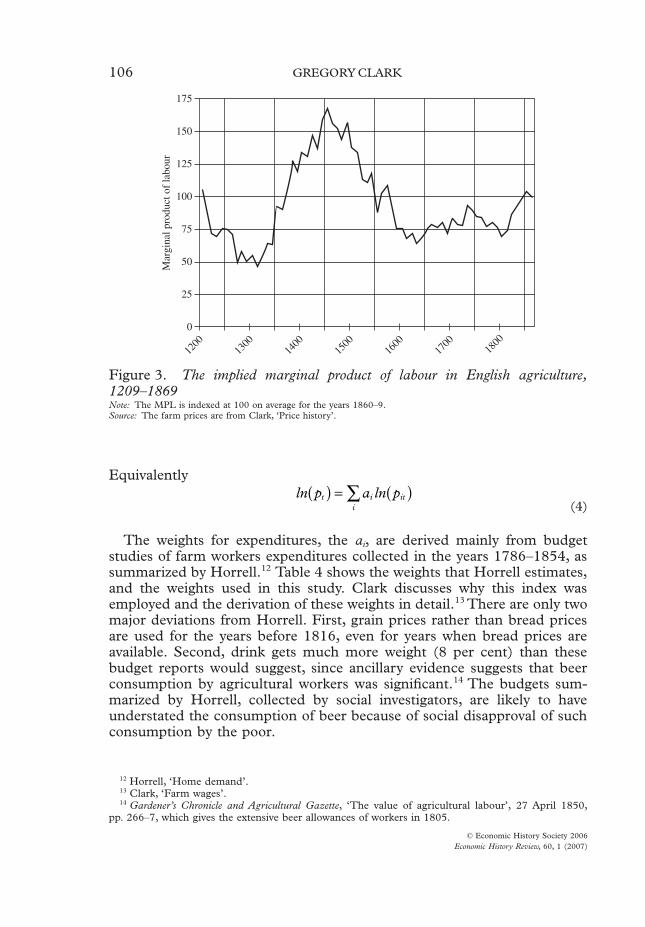
The assumption that medieval cultivators acted in such a way as to meetthis condition may seem fanciful, but after the Black Death when theimplied MPL rose very substantially we see that the implied threshing,reaping, and mowing work rates rose substantially, then declined againwhen the MPL fell. Thus even medieval cultivators seem to have respondedto labour costs in deciding how carefully to have workers perform tasks. Soit is not implausible that the wage divided by product prices will indicatethe MPL even in 1300. The MPL matters for considerations of technologi-cal advance in agriculture. Figure 3 shows an index of the MPL, whichis just nominal wages divided by this output price index, with the years1860–9 set to 100.
11
The second real wage measure is the purchasing power of farm wages forthe workers: the amount the day wage could buy of the goods consumedby farm workers, which included, importantly, candles, soap, shoes, textiles,housing, tea, and sugar produced outside the domestic agricultural sector.This measures the standard of living of farm workers. These two wagemeasures can in principle differ substantially, and do indeed differ for theseyears.
The farm workers’ cost of living index is formed as a geometric index ofthe prices of each component, with expenditure shares used as weights. Itthus assumes constant shares of expenditure on each item as relative priceschange. That is, if
p
it
is the price index for each commodity
i
in year
t
, and
a
i
is the expenditure share of commodity
i
, then the overall price level ineach year,
p
t
is calculated as,
(3)
where
n
is the number of good consumed.
10
Strictly, farmers must be acting as though to maximize profits and must take the wage they face asgiven.
11
The price index is from Clark, ‘Price history’.
w p MPL= ¥
MPLwp
=
p p p p pt ita a a
na
i
i n= =’ 1 21 2 . . . . .
106
GREGORY CLARK
© Economic History Society 2006
Economic History Review
, 60, 1 (2007)
Equivalently
(4)
The weights for expenditures, the ai, are derived mainly from budgetstudies of farm workers expenditures collected in the years 1786–1854, assummarized by Horrell.12 Table 4 shows the weights that Horrell estimates,and the weights used in this study. Clark discusses why this index wasemployed and the derivation of these weights in detail.13 There are only twomajor deviations from Horrell. First, grain prices rather than bread pricesare used for the years before 1816, even for years when bread prices areavailable. Second, drink gets much more weight (8 per cent) than thesebudget reports would suggest, since ancillary evidence suggests that beerconsumption by agricultural workers was significant.14 The budgets sum-marized by Horrell, collected by social investigators, are likely to haveunderstated the consumption of beer because of social disapproval of suchconsumption by the poor.
12 Horrell, ‘Home demand’.13 Clark, ‘Farm wages’.14 Gardener’s Chronicle and Agricultural Gazette, ‘The value of agricultural labour’, 27 April 1850,
pp. 266–7, which gives the extensive beer allowances of workers in 1805.
ln lnp a pt i iti
( ) = ( )Â
Figure 3. The implied marginal product of labour in English agriculture,1209–1869Note: The MPL is indexed at 100 on average for the years 1860–9.Source: The farm prices are from Clark, ‘Price history’.
175
150
125
100
75
50
25
0
Mar
gina
l pro
duct
of
labo
ur
1200
1300
1400
1500
1600
1700
1800

THE LONG MARCH OF HISTORY 107
© Economic History Society 2006Economic History Review, 60, 1 (2007)
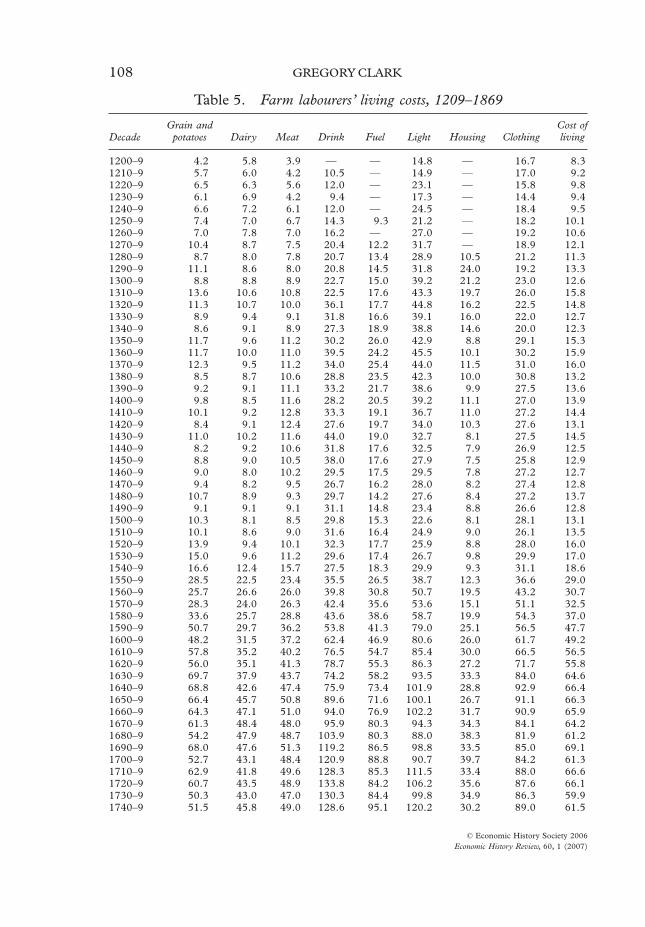
Since, as we shall see, real living standards of farm workers generally laywithin 50 per cent of living standards in 1787–1854, the period that gave usthe budget weights, a fixed set of weights is used throughout. There are 36items in the cost-of-living index, including such exotica as stockings, gloves,and trenchers, which were amalgamated into 12 subcategories: grains andpotato, dairy, meats, sugars, drink, salt, fuel, light, soap, clothing, lodging, andservices, with the weights given to each shown in table 4. Some of items, suchas potatoes and cane sugar (as opposed to honey), only appear later. Table 5reports by decade the values of the more important of these sub-indices, andthe cost of living index as a whole, with 1860–9 set to 100 in each case.15
15 Clark, ‘Price history’ gives the annual prices and the sources of the 16 domestic farmproduced items in the cost of living index: wheat, barley, oats, peas, potatoes, cheese, butter, milk, beef,mutton, pork, bacon, suet, eggs, cider, and firewood. Clark, ‘Condition of the working class’, tab. A4,pp. 1330–32, gives the sources for the other 20 items: fish, beer, tea, sugar, candles, coal gas, soap,coal, charcoal, salt, shoes, gloves, stockings, wool cloth, linen cloth, cotton cloth, housing, trenchers,pewter, and services. Housing here is estimated as the rental cost of housing of standard quality forareas outside London.
Table 4. The percentage of expenditure by category for farm labourers before 1869
Category of expenditure 1787–96 (Horrell) 1840–54 (Horrell) Assumed here
Food and Drink: 77.0 68.6 73.0Bread and flour 40.1 33.5 0.0Wheat 0.0 3.0 40.0Barley 1.0 1.4 3.0Oats and oatmeal 3.6 2.2 2.5Peas — — 2.5Potato 2.0 6.0 4.0Meat 9.2 3.4 10.5Fish 0.0 0.0 0.0Bacon 1.3 2.8 1.0Eggs 0.0 0.0 0.5Milk 4.0 3.2 4.3Cheese 3.5 2.6 2.3Butter 3.9 3.3 5.1Sugar and honey 3.6 3.1 3.0Beer 0.0 0.0 4.7Tea 2.4 2.6 3.3Coffee 0.0 0.0 0.0Salt — — 0.5Other food 1.4 1.6 0.0
Housing 6.0 10.1 6.0Fuel 4.0 4.5 5.0Light — — 3.5Soap — — 0.5Services 0.1 0.7 0.5Tobacco 0.0 1.0 0.0Other (clothing, bed linen) 8.2 11.7 10.0
Source: Horrell, ‘Home demand’, pp. 568–9, 577.
108 GREGORY CLARK
© Economic History Society 2006Economic History Review, 60, 1 (2007)
Table 5. Farm labourers’ living costs, 1209–1869
DecadeGrain and
potatoes Dairy Meat Drink Fuel Light Housing ClothingCost ofliving
1200–9 4.2 5.8 3.9 — — 14.8 — 16.7 8.31210–9 5.7 6.0 4.2 10.5 — 14.9 — 17.0 9.21220–9 6.5 6.3 5.6 12.0 — 23.1 — 15.8 9.81230–9 6.1 6.9 4.2 9.4 — 17.3 — 14.4 9.41240–9 6.6 7.2 6.1 12.0 — 24.5 — 18.4 9.51250–9 7.4 7.0 6.7 14.3 9.3 21.2 — 18.2 10.11260–9 7.0 7.8 7.0 16.2 — 27.0 — 19.2 10.61270–9 10.4 8.7 7.5 20.4 12.2 31.7 — 18.9 12.11280–9 8.7 8.0 7.8 20.7 13.4 28.9 10.5 21.2 11.31290–9 11.1 8.6 8.0 20.8 14.5 31.8 24.0 19.2 13.31300–9 8.8 8.8 8.9 22.7 15.0 39.2 21.2 23.0 12.61310–9 13.6 10.6 10.8 22.5 17.6 43.3 19.7 26.0 15.81320–9 11.3 10.7 10.0 36.1 17.7 44.8 16.2 22.5 14.81330–9 8.9 9.4 9.1 31.8 16.6 39.1 16.0 22.0 12.71340–9 8.6 9.1 8.9 27.3 18.9 38.8 14.6 20.0 12.31350–9 11.7 9.6 11.2 30.2 26.0 42.9 8.8 29.1 15.31360–9 11.7 10.0 11.0 39.5 24.2 45.5 10.1 30.2 15.91370–9 12.3 9.5 11.2 34.0 25.4 44.0 11.5 31.0 16.01380–9 8.5 8.7 10.6 28.8 23.5 42.3 10.0 30.8 13.21390–9 9.2 9.1 11.1 33.2 21.7 38.6 9.9 27.5 13.61400–9 9.8 8.5 11.6 28.2 20.5 39.2 11.1 27.0 13.91410–9 10.1 9.2 12.8 33.3 19.1 36.7 11.0 27.2 14.41420–9 8.4 9.1 12.4 27.6 19.7 34.0 10.3 27.6 13.11430–9 11.0 10.2 11.6 44.0 19.0 32.7 8.1 27.5 14.51440–9 8.2 9.2 10.6 31.8 17.6 32.5 7.9 26.9 12.51450–9 8.8 9.0 10.5 38.0 17.6 27.9 7.5 25.8 12.91460–9 9.0 8.0 10.2 29.5 17.5 29.5 7.8 27.2 12.71470–9 9.4 8.2 9.5 26.7 16.2 28.0 8.2 27.4 12.81480–9 10.7 8.9 9.3 29.7 14.2 27.6 8.4 27.2 13.71490–9 9.1 9.1 9.1 31.1 14.8 23.4 8.8 26.6 12.81500–9 10.3 8.1 8.5 29.8 15.3 22.6 8.1 28.1 13.11510–9 10.1 8.6 9.0 31.6 16.4 24.9 9.0 26.1 13.51520–9 13.9 9.4 10.1 32.3 17.7 25.9 8.8 28.0 16.01530–9 15.0 9.6 11.2 29.6 17.4 26.7 9.8 29.9 17.01540–9 16.6 12.4 15.7 27.5 18.3 29.9 9.3 31.1 18.61550–9 28.5 22.5 23.4 35.5 26.5 38.7 12.3 36.6 29.01560–9 25.7 26.6 26.0 39.8 30.8 50.7 19.5 43.2 30.71570–9 28.3 24.0 26.3 42.4 35.6 53.6 15.1 51.1 32.51580–9 33.6 25.7 28.8 43.6 38.6 58.7 19.9 54.3 37.01590–9 50.7 29.7 36.2 53.8 41.3 79.0 25.1 56.5 47.71600–9 48.2 31.5 37.2 62.4 46.9 80.6 26.0 61.7 49.21610–9 57.8 35.2 40.2 76.5 54.7 85.4 30.0 66.5 56.51620–9 56.0 35.1 41.3 78.7 55.3 86.3 27.2 71.7 55.81630–9 69.7 37.9 43.7 74.2 58.2 93.5 33.3 84.0 64.61640–9 68.8 42.6 47.4 75.9 73.4 101.9 28.8 92.9 66.41650–9 66.4 45.7 50.8 89.6 71.6 100.1 26.7 91.1 66.31660–9 64.3 47.1 51.0 94.0 76.9 102.2 31.7 90.9 65.91670–9 61.3 48.4 48.0 95.9 80.3 94.3 34.3 84.1 64.21680–9 54.2 47.9 48.7 103.9 80.3 88.0 38.3 81.9 61.21690–9 68.0 47.6 51.3 119.2 86.5 98.8 33.5 85.0 69.11700–9 52.7 43.1 48.4 120.9 88.8 90.7 39.7 84.2 61.31710–9 62.9 41.8 49.6 128.3 85.3 111.5 33.4 88.0 66.61720–9 60.7 43.5 48.9 133.8 84.2 106.2 35.6 87.6 66.11730–9 50.3 43.0 47.0 130.3 84.4 99.8 34.9 86.3 59.91740–9 51.5 45.8 49.0 128.6 95.1 120.2 30.2 89.0 61.5
Note: The index for each commodity and overall is set to 100 for 1860–9.
THE LONG MARCH OF HISTORY 109
© Economic History Society 2006Economic History Review, 60, 1 (2007)
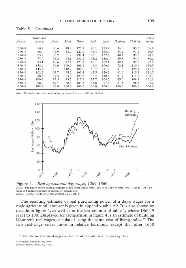
The resulting estimate of real purchasing power of a day’s wages for amale agricultural labourer is given in appendix table A2. It is also shown bydecade in figure 4, as well as in the last column of table 1, where 1860–9is set to 100. Displayed for comparison in figure 4 is an estimate of buildinglabourer’s real wages calculated using the same cost of living index.16 Thetwo real-wage series move in relative harmony, except that after 1650
16 The labourers’ nominal wages are from Clark, ‘Condition of the working class’.
1750–9 60.2 46.6 49.8 125.9 96.1 115.9 34.0 93.5 66.81760–9 66.0 47.9 54.2 127.9 96.4 125.0 34.7 97.2 70.91770–9 75.2 55.2 61.9 137.4 103.1 132.4 40.4 95.3 78.71780–9 77.0 57.3 64.1 132.2 103.2 138.4 39.5 94.9 80.21790–9 93.1 68.6 77.1 123.9 116.1 152.1 49.4 97.2 92.91800–9 133.4 96.9 109.9 161.1 146.4 196.6 72.1 110.9 126.51810–9 145.4 118.1 118.2 180.0 158.7 211.2 91.6 122.1 141.21820–9 102.7 103.7 95.5 163.4 142.5 129.3 91.9 115.7 111.51830–9 98.6 97.5 83.4 129.7 132.4 110.4 91.7 111.5 103.31840–9 100.9 95.3 83.5 115.9 117.7 104.5 85.0 108.8 101.11850–9 98.0 87.7 88.4 104.3 103.6 97.8 87.5 96.5 96.21860–9 100.0 100.0 100.0 100.0 100.0 100.0 100.0 100.0 100.0
DecadeGrain and
potatoes Dairy Meat Drink Fuel Light Housing ClothingCost ofliving
Note: The index for each commodity and overall is set to 100 for 1860–9.
Table 5. Continued
Figure 4. Real agricultural day wages, 1209–1869Notes: The figure shows decadal averages of real farm wages from 1200–9 to 1860–9, with 1860–9 set to 100. The wage of building labourers is shown for comparison.Source: Clark, ‘Condition of the working class’, tab. 1.
160
140
120
100
80
60
40
20
0
Rea
l wag
e (1
860s
= 1
00)
1200
1300
1400
1500
1600
1700
1800
Farm labourers
Buildinglabourers
110 GREGORY CLARK
© Economic History Society 2006Economic History Review, 60, 1 (2007)
building wages gained steadily relative to those of farm labourers. Indeed,in the earlier years, such as 1400–1500, farm labourers often earned morethan building labourers. By the nineteenth century, farm labourers earnedonly 78 per cent of the wages of building labourers. Thus the premium ofthe building workers, many more of whom were located in towns, was inthe order of 25 per cent or less over this long interval. Given higher housing,food, and fuel costs in towns, the differences in standards of living wereeven smaller than this.
Since the gap between farm and building wages increases somewhat overtime, we see that there is no sign of any better integration of the labourmarket by the nineteenth century than there was in the thirteenth century.There is certainly no sign of a ‘dual’ labour market in pre-industrial Englandsuch as has been posited for modern pre-industrial economies.
Farm workers had the lowest real wages in the recorded history ofEngland around 1300. Indeed, the worst year on record is 1316, when realday wages were just 29 per cent of their average level in the 1860s. Thesecond worst year, at 32 per cent, was 1317, explaining the Great Famineof these years. But 1310–11 and 1322–23 also saw successive years of realwages at 36 per cent or below of the 1860s. Thus 1310–23 saw six of theseven worst years of real wages in recorded history, 1296 being the seventhyear. Wages from 1290–1319 averaged one-third less than those in the nextlow point in wage history, in the early seventeenth century. By the 1760sand the eve of the Industrial Revolution, real day wages had increased byabout 70 per cent from the pre-Black Death trough.
England had one of the most efficient agricultures in the world by 1850.Indeed it was the high labour productivity of English agriculture, in part,that allowed the share of labour employed in agriculture to fall so much inthe Industrial Revolution era. But there has been continued debate aboutwhen, and how, output per worker increased. Some have favoured theIndustrial Revolution era, others the seventeenth century, and yet othershave argued that high output per worker was achieved by the later middleages. Thus, at one extreme, Eona Karakacili recently presented data froma medieval estate implying that output per man-day in arable agriculturebefore the Black Death ‘either surpassed or met the literature’s best esti-mates for English workers until 1800’ and was respectable even by thestandards of 1850.17 At another extreme, recently E. A. Wrigley adducedevidence based on overall yields per acre and the presumed numbers ofworkers per acre that suggest output per worker in 1800 was 3–4 times thatin 1300.18
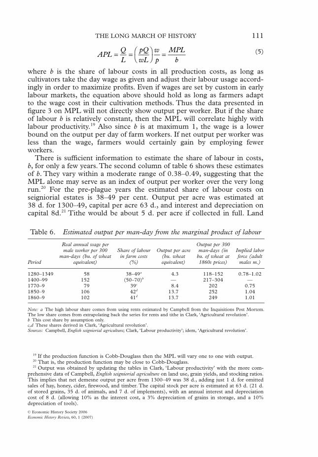
The MPL series derived above casts new light on this issue. Output perman-day, the average product of labour (APL), is connected to the MPL,by the simple formula
17 Karakacili, ‘Agrarian labour productivity’, p. 24.18 Wrigley, ‘Transition’, p. 31. Clark, ‘Labour productivity’, earlier made a similar estimate. For an
estimate intermediate between these and Karakacili, see Allen, ‘Economic structure’.
THE LONG MARCH OF HISTORY 111
© Economic History Society 2006Economic History Review, 60, 1 (2007)
(5)
where b is the share of labour costs in all production costs, as long ascultivators take the day wage as given and adjust their labour usage accord-ingly in order to maximize profits. Even if wages are set by custom in earlylabour markets, the equation above should hold as long as farmers adaptto the wage cost in their cultivation methods. Thus the data presented infigure 3 on MPL will not directly show output per worker. But if the shareof labour b is relatively constant, then the MPL will correlate highly withlabour productivity.19 Also since b is at maximum 1, the wage is a lowerbound on the output per day of farm workers. If net output per worker wasless than the wage, farmers would certainly gain by employing fewerworkers.
There is sufficient information to estimate the share of labour in costs,b, for only a few years. The second column of table 6 shows these estimatesof b. They vary within a moderate range of 0.38–0.49, suggesting that theMPL alone may serve as an index of output per worker over the very longrun.20 For the pre-plague years the estimated share of labour costs onseigniorial estates is 38–49 per cent. Output per acre was estimated at38 d. for 1300–49, capital per acre 63 d., and interest and depreciation oncapital 8d.21 Tithe would be about 5 d. per acre if collected in full. Land
19 If the production function is Cobb-Douglass then the MPL will vary one to one with output.20 That is, the production function may be close to Cobb-Douglass.21 Output was obtained by updating the tables in Clark, ‘Labour productivity’ with the more com-
prehensive data of Campbell, English seigniorial agriculture on land use, grain yields, and stocking ratios.This implies that net demesne output per acre from 1300–49 was 38 d., adding just 1 d. for omittedsales of hay, honey, cider, firewood, and timber. The capital stock per acre is estimated at 63 d. (21 d.of stored grains, 35 d. of animals, and 7 d. of implements), with an annual interest and depreciationcost of 8 d. (allowing 10% as the interest cost, a 3% depreciation of grains in storage, and a 10%depreciation of tools).
APLQL
pQwL
wp
MPLb
= = ÊË
ˆ¯ =
Table 6. Estimated output per man-day from the marginal product of labour
Period
Real annual wage permale worker per 300
man-days (bu. of wheatequivalent)
Share of labourin farm costs
(%)
Output per acre(bu. wheatequivalent)
Output per 300man-days (in
bu. of wheat at1860s prices)
Implied laborforce (adultmales m.)
1280–1349 58 38–49a 4.3 118–152 0.78–1.021400–99 152 (50–70)b — 217–304 —1770–9 79 39c 8.4 202 0.751850–9 106 42d 13.7 252 1.041860–9 102 41d 13.7 249 1.01
Note: a The high labour share comes from using rents estimated by Campbell from the Inquisitions Post Mortem.The low share comes from extrapolating back the series for rents and tithe in Clark, ‘Agricultural revolution’.b This cost share by assumption only.c,d These shares derived in Clark, ‘Agricultural revolution’.Sources: Campbell, English seigniorial agriculture; Clark, ‘Labour productivity’; idem, ‘Agricultural revolution’.

112 GREGORY CLARK
© Economic History Society 2006Economic History Review, 60, 1 (2007)
rents can be estimated in two ways. Based on the Inquisitions Post Mortem,which probably understate values, rents per acre averaged 6 d. or less,producing a joint rent and tithe share of 29 per cent, and a labour share of49 per cent.22 An alternative estimate, extrapolating back the rent series withfresh data for the years before, suggests a higher value for rent and tithe of15.5 d. per acre, and a labour share of only 38 per cent.23
Applying these share estimates to the MPL gives the new, more optimis-tic, estimate of labour productivity c.1300 shown in table 6. The gains from1300 to 1800 were only 33–70 per cent. But these estimates suggest thatthere was no reasonable share of labour in costs that would make medievallabour productivity as high as in the 1770s, as Karakacili argues, given thesubstantially lower MPL in 1300 than in 1770. This still means, however,that agricultural output per worker in pre-plague England was as high as inmost European countries, such as France or Ireland, in the mid-nineteenthcentury.24
Are these new estimates feasible, and why do they not match the earlierestimates of Clark, and the recent ones of Wrigley? The first check is againstthe implied productivity of labour on specific tasks given by piece rates forthreshing grains, mowing grass, and reaping wheat. As Clark pointed out,it is puzzling that the task specific estimates of labour productivity for themajor tasks in agriculture, which absorbed 40–50 per cent of all male labourinputs, showed little gains between 1300 and 1800 or even 1850–60.25
Table 7, for example, shows estimated (net) output per worker inthreshing wheat, reaping wheat, and mowing meadow in 1300–49,1400–49, 1768–71, 1794–1806, 1850, and 1860. In threshing labour pro-ductivity declines between 1300 and 1770–1860, in reaping it gains byabout 70 per cent, and in mowing by about 80 per cent. Aggregating acrossthese tasks, there was no more than a 25 per cent gain in labour productivity.
22 This estimate assumes that arable rented at 4.7 d. per acre on average, and pasture and meadowat 12 d. per acre. See Campbell, English seigniorial agriculture.
23 Clark, ‘Agricultural revolution’.24 Clark, ‘Labour productivity’, p. 213, gives estimates for these other countries c.1850.25 Clark, ‘Labour productivity’, pp. 221–31.
Table 7. Task-specific labour productivities
PeriodThreshing Wheat
(bu./day)Reaping Wheat – net
output (bu./day)Mowing Meadow
(acre/day)
1300–49 5.1 4.5 0.511400–49 7.3 6.2 0.681768–71 4.2 7.9 0.941794–1806 4.3 8.6 1.021850 3.9 7.6 0.861860 — 7.9 0.83
Source: Clark, ‘Labour productivity’, and the text.
THE LONG MARCH OF HISTORY 113
© Economic History Society 2006Economic History Review, 60, 1 (2007)
Nothing here supports substantial gains, everything supports limited labourproductivity gains.
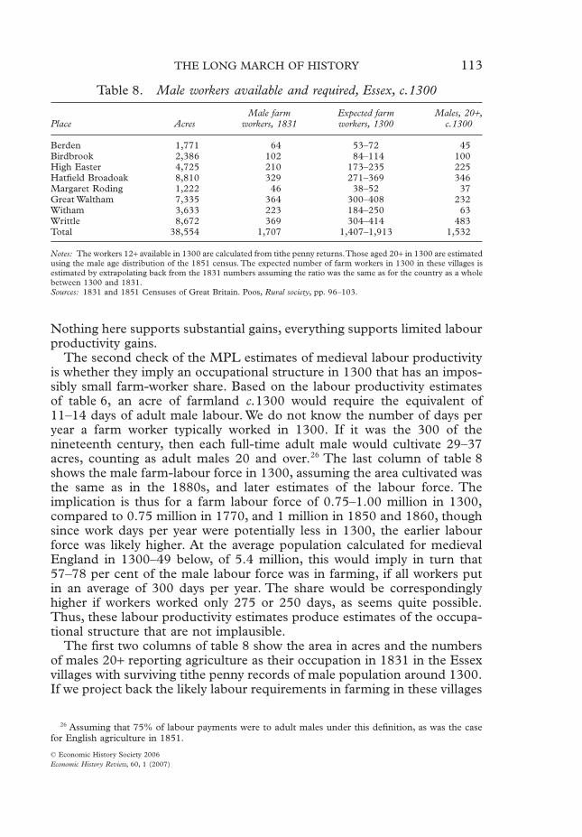
The second check of the MPL estimates of medieval labour productivityis whether they imply an occupational structure in 1300 that has an impos-sibly small farm-worker share. Based on the labour productivity estimatesof table 6, an acre of farmland c.1300 would require the equivalent of11–14 days of adult male labour. We do not know the number of days peryear a farm worker typically worked in 1300. If it was the 300 of thenineteenth century, then each full-time adult male would cultivate 29–37acres, counting as adult males 20 and over.26 The last column of table 8shows the male farm-labour force in 1300, assuming the area cultivated wasthe same as in the 1880s, and later estimates of the labour force. Theimplication is thus for a farm labour force of 0.75–1.00 million in 1300,compared to 0.75 million in 1770, and 1 million in 1850 and 1860, thoughsince work days per year were potentially less in 1300, the earlier labourforce was likely higher. At the average population calculated for medievalEngland in 1300–49 below, of 5.4 million, this would imply in turn that57–78 per cent of the male labour force was in farming, if all workers putin an average of 300 days per year. The share would be correspondinglyhigher if workers worked only 275 or 250 days, as seems quite possible.Thus, these labour productivity estimates produce estimates of the occupa-tional structure that are not implausible.
The first two columns of table 8 show the area in acres and the numbersof males 20+ reporting agriculture as their occupation in 1831 in the Essexvillages with surviving tithe penny records of male population around 1300.If we project back the likely labour requirements in farming in these villages
26 Assuming that 75% of labour payments were to adult males under this definition, as was the casefor English agriculture in 1851.
Table 8. Male workers available and required, Essex, c.1300
Place AcresMale farm
workers, 1831Expected farmworkers, 1300
Males, 20+,c.1300
Berden 1,771 64 53–72 45Birdbrook 2,386 102 84–114 100High Easter 4,725 210 173–235 225Hatfield Broadoak 8,810 329 271–369 346Margaret Roding 1,222 46 38–52 37Great Waltham 7,335 364 300–408 232Witham 3,633 223 184–250 63Writtle 8,672 369 304–414 483Total 38,554 1,707 1,407–1,913 1,532
Notes: The workers 12+ available in 1300 are calculated from tithe penny returns. Those aged 20+ in 1300 are estimatedusing the male age distribution of the 1851 census. The expected number of farm workers in 1300 in these villages isestimated by extrapolating back from the 1831 numbers assuming the ratio was the same as for the country as a wholebetween 1300 and 1831.Sources: 1831 and 1851 Censuses of Great Britain. Poos, Rural society, pp. 96–103.
114 GREGORY CLARK
© Economic History Society 2006Economic History Review, 60, 1 (2007)
in 1300, based on the estimated sizes of the farm labour force nationally in1300 and 1831, we get the numbers in the next column. These are thenumbers of farm labourers we would expect to see in these communities in1300, based on our labour productivity estimate. The final column showsthe numbers of 20+ age males available based on the work of Larry Pooson the tithing penny records. As can be seen, even at the high labourproductivities posited for 1300, the expected farm labour requirement of1,407–1,913 males would absorb nearly the entire male population of thesevillages of 1,532. Again, the new labour productivity estimates are plausible.
Lastly, if these new medieval labour productivity estimates seem plausible,why do Wrigley and Clark (earlier) produce much lower estimates? Wrigleyestimates about the same numbers of farm workers in medieval England asis estimated here.27 But he has a low estimate of total output because hefollows Campbell in assuming only 6.7 million sown acres out of a totalcultivable area in England of 26.5 million acres.28 This generates a lowestimate of output per worker. When we discuss population below we shallsee that the assumption of only 6.7 million sown acres is too low. Clarkestimates workers per sown acre from estimates of households per sown acreas with Kosminsky’s analysis of the Hundred Rolls of 1279–80.29 The totalnumber of acres per worker is calculated in this way as 11–15, which generatesthe low labour productivity estimates. But these estimates are less securethan the MPL estimates and the output per acre estimates used above, sincethey involve many ancillary assumptions: the average size of the household,the proportion employed in agriculture, the ratio of sown to all acres.
A remaining puzzle is why, if labour productivity was comparatively highin medieval England, were urbanization rates so low, at less than 5 per cent?The lack of urbanization, indeed, is a feature that Wrigley takes as support-ing low labour productivity c.1300.30 For if agricultural labour productivitywas high, so that each farm worker can feed many non-farm workers, thenso also should the share of workers in non-agricultural occupations havebeen high. And these workers, not being attached to the land, typicallylocate in towns and cities. The significant gains in urbanization in Englandbetween 1300 and 1800, from 3 per cent to 20 per cent, seemingly suggestmuch greater farm labour productivity by the latter years. This puzzle is infact greater for 1450 than for 1300. For by 1450 there is no possibility thatlabour productivity could have been any less than in 1770 or 1800. Astable 6 reveals, farm workers’ day wages then were alone three quarters ofoutput per worker in 1770. Why did the undoubted rise in output per workerafter the plague not lead to a significant gain in urbanization?
The measure of urbanization used above, however, is the proportion ofthe population in towns of 10,000 or more. Dyer has argued that if all towns
27 Wrigley, ’Transition’.28 Campbell, English seigniorial agriculture.29 Clark, ‘Labour productivity’.30 Wrigley, ‘Urban growth’, p. 71.
THE LONG MARCH OF HISTORY 115
© Economic History Society 2006Economic History Review, 60, 1 (2007)
are included then 15–20 per cent of England was urbanized in 1300.31 Hethus argues that England had an unusual urban structure, with many moresmall urban locations. This might be created, for example, by Englandhaving an unusual degree of security from organized violence in the middleages, so that security as a motive for larger urban agglomerations was absent.Thus overall there seems no compelling reason to reject the MPL estimatesof figure 3 as offering a guide to likely output per worker in agriculture overthe long run.
Below I estimate population in medieval England using the MPL to proxyfor population. To do this I need one further assumption to hold. This isthat the agricultural wage tended to clear the labour market, and at least toan approximation balanced labour supplies with labour demands. Inparticular, wages cannot be set by some customary standard. Many scholarsof the middle ages will be sceptical of this assumption.32 Since this isimportant for what follows, let us consider nominal wages in the years1280–1440, where wage quotes are plentiful, and ask whether the evidenceof these years supports or contradicts the assumption that wages adjustedto match demand and supply of labour.
If nominal wages moved up and down regularly in these years, therewould be no question of their flexibility. However, there were long periodsin which nominal wages were stable, 1270–1315 for example, and very fewperiods in which nominal wages fell. The stability of nominal wages overlong periods does not in itself imply that markets failed to work. Labourdemand and supply might just have happened to be in balance at thosenominal wages for long periods. But their stability makes it harder to beconfident that a relatively free labour market indeed operated.
The presence of sudden population losses in the medieval years causedby plague, as in 1348–9, and famine, as in 1316–17, however, allows oneto check whether wages rapidly responded to changes in supplies as wewould expect in a competitive market, or whether wages failed to adjust, oradjusted slowly, since nominal wages were governed strongly by custom.
Sudden losses of population should create an immediate increase innominal wages if labour markets were competitive, for two reasons. The firstis that the population decline would reduce real output, Y. As long as themoney supply (M) and the velocity of circulation of money (V ) is unaffectedby the population loss, then since
the price level P would have increased.33 Nominal wages would have toproportionately increase to maintain real wages. But since the demographic
31 Dyer, Everyday life, p. 302.32 John Munro, for one, has argued strongly against such an assumption, viewing building workers’
wages as having adjusted slowly to economic conditions. Munro, ‘Wage stickiness’; idem, ‘Postan’.33 Not all prices need rise since there would be important changes in relative prices after a demographic
shock, with farm output becoming relatively cheaper and manufactured output becoming moreexpensive.
MV PY=
116 GREGORY CLARK
© Economic History Society 2006Economic History Review, 60, 1 (2007)
decline makes labour scarce relative to land and capital, real wages shouldrise in a competitive market, causing further upward movement of nominalwages. Thus, any sudden fall in population should immediately increasemoney wages.
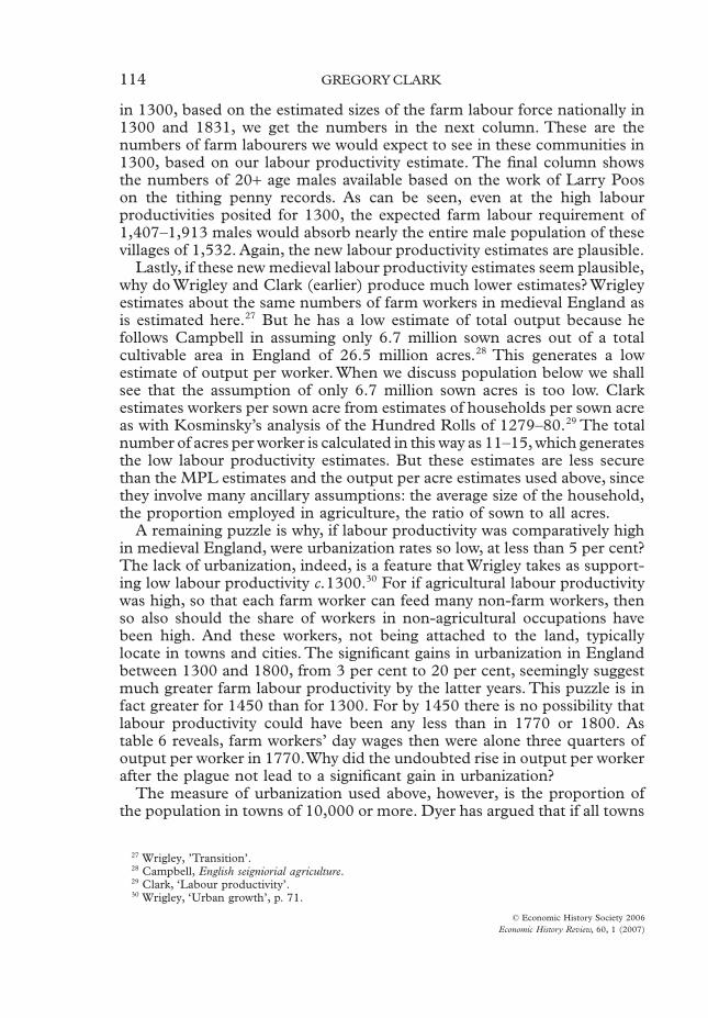
Figure 5, which shows the estimated nominal wage in each year for1280–1440, attempts to detect whether demographic shocks led to suddenadjustments of nominal wages for the years where we have the best wagemeasures. Even with a lot of data, there is still a sampling error in the wageestimate for any year, so that the line is not as smooth as the true averagewage series would be. But the movement of the series is characterized by anumber of relatively abrupt wage changes followed by long periods ofstability. These breaks, which are all statistically highly significant, so thatthey cannot be attributed to chance, are also shown in figure 5. Theyoccurred around 1316, 1350, 1352, 1364, 1372, 1389, 1399, and 1424.
The experience in both 1316 and 1350 is suggestive that wages werecertainly flexible upwards and by the degree we would expect in a com-petitive market. In 1316 nominal wages rose to a new level, 14 per centabove the pre-famine level. This is consistent with the widespread notionthat population losses in the famine of 1315–7 were in the order of 10 percent. The immediate effect of the Black Death in 1348–9 was a rise in wagesof 101 per cent by 1350, a rise that began in 1349. Clearly nominal wageswere again highly responsive to this shock, and with a magnitude that isconsistent with the typical estimate of a 25–40 per cent population loss.
Figure 5. Changes in the nominal wage series, 1280–1440Notes: The breaks in the series seem to come in 1316, 1350, 1352, 1364, 1372, 1389, 1399, and 1424.Source: See text.
Nom
inal
wag
es, 1
280-
1440
1440
1420
1400
1380
1360
1340
1320
1300
1280
0
0.5
1
1.51316
1364
13501372
1389
13991424
2
2.5
3
3.5
4
THE LONG MARCH OF HISTORY 117
© Economic History Society 2006Economic History Review, 60, 1 (2007)
Interestingly, though, the wage level fell back by about 14 per centbetween 1351 and 1352. The Statute of Labourers of 1351, whichtheoretically fixed wages at pre-plague levels, may thus have depressedreported wages below their market clearing levels, at least for a few years,though the effect was clearly modest, even in the short run. The statuteexplicitly, for example, called for payments for threshing wheat to be nomore than 2.5 d. per quarter. Of 20 manors reporting wheat threshingpayments in 1352 or 1353, only five had rates sanctioned by the Statute.Even if the Statute repressed reported wages it does not imply that the wagespaid were really below the market clearing rate, for there were many waysof making side payments to workers through food and other gifts to bringup low nominal wages to the market rate. So the Statute may well have hadan effect only on the form of wages, not on the total wage paymentsthemselves. But it does suggest that at least in the 1350s reported wagesmay well understate market rates. Over time we can assume that distortionsin reported wages stemming from the Statute diminished gradually.
After 1352 there were four years in which the data suggest a relativelyrapid upward movement in wages to a new level: 1364, 1372, 1399, and1424. These correspond loosely, but not precisely, to later reported plagueepidemics, and many reported plague episodes in these years have no effecton wages. Thus national plague outbreaks are reported for 1361–2, 1369,1375, 1379–83, 1390–1, 1399–1400, 1405–6, 1411–12, 1420–3, 1426–9,1433–5, and 1438–9.34 We have little idea of the relative severity of thesevarious plague outbreaks, so the nominal wage behaviour in response tothese may just reflect their comparative impacts on population. But thecoordinated upwards movement of nominal wages across a range of loca-tions in short periods does suggest that wages were again flexible upwardsin response to labour market shocks.
The decline in wages around 1389 might seemingly prove that nominalwages were also flexible downwards. But the cause is a little mysterious.Population cannot grow suddenly, to cause a sudden nominal wage decline.There can be rapid contractions in the nominal money supply, which would,in a competitive market, lead to a drop in nominal wages. But we have noindependent evidence of such a contraction in 1389.
Thus the verdict on medieval labour markets is that wages certainlydisplay upward flexibility. That they were downwardly flexible is less easyto demonstrate since on only two occasions in the years 1270–1450 didwages clearly decline. The decline in 1352 may well have been due to theStatute of Labourers, so there is only one decline attributable to marketforces. Also, the Statute of Labourers may have depressed reported wagesbelow market clearing wages in the 1350s, so that in this decade reportedwages were too low, though most likely by 14 per cent or less. In the years1320–50 the money supply in England seems to have declined signifi-
34 See Gottfried, Black Death; Shrewsbury, Bubonic plague.
118 GREGORY CLARK
© Economic History Society 2006Economic History Review, 60, 1 (2007)
cantly.35 In response, average prices fell also, but nominal wages did notdecline. Thus real wages rose. Below I attribute that to a decline in popu-lation from 1320–49, but if nominal wages were inflexible downwards, thesemovements in the money base will produce, for some periods, misleadingimplications about the likely population of England. But in periods such as1350–1430, with persistent upward movement of nominal wages, the wagecan be assumed to reflect labour supply and demand.
II
Huge swings in the MPL are evident over time in figure 3. The MPL variesfrom 85 per cent of the level of the 1860s before 1270, to only about halfthe level in 1270–1329, to 150 per cent of the level in the fifteenth century.The earlier movements are inversely related to estimated population levels.Thus we get little idea about agricultural efficiency gains from looking atoutput per worker alone, or the MPL, unless we also have measures ofearlier populations.
Unfortunately, English population before 1540, when parish registerestimates become available, is uncertain. Population estimates for 1300–15,when the medieval population is believed to have been at its maximum,have ranged from 4 million to 6.5 million. Bruce Campbell recently pro-nounced in favour of a maximum medieval population of 4–4.25 million in1300–49, based on estimates of the total food output in England. Butothers, such as Richard Smith, relying on the extent of populationlosses in the handful of communities for which we have evidence for theyears 1300–1500, have estimated a much bigger maximum population of6 to 6.5 million people.36
Figure 3 shows that in 1600–19, when population averaged 4.6 million,the MPL was nearly 50 per cent higher than in 1300. If England in 1300had a population of only 4 million, then there were substantial agriculturalefficiency gains between 1300 and 1600. If, however, the population in 1300was 6 million, then it is possible that there were no efficiency gains over thislong interval of 300 years.
Below, population trends for the medieval period for the years 1200–1530are estimated from the records of 21 medieval communities. When wecompare this population trend to the MPL series for the years 1250–1530,the two series correlate highly. This suggests these ‘micro’ population esti-mates are correctly capturing the general population trend, and that agri-cultural technology was static in these years. To get a long-run estimate ofpopulation levels in England we still need to fix the level of population atsome point before 1530. By making the modest assumption of no changein agricultural technology between the end of the ‘micro’ level populationevidence in the 1520s and the start of national population estimates in the
35 Allen, ‘Volume of the English currency’.36 Campbell, English seigniorial agriculture, pp. 403–5; Smith, ‘Human resources’, pp. 189–91.

THE LONG MARCH OF HISTORY 119
© Economic History Society 2006Economic History Review, 60, 1 (2007)
1540s, we can fix earlier populations using the MPL. With just this assump-tion of the MPL, national population levels of the 1540s to 1610s andcommunity level estimates for 1250–1529 all fit together, and imply a statictechnology from 1250 to at least 1600.
Evidence for population trends in communities in the medieval periodcomes in two main forms. The first type of estimate, favoured byRaftis and his ‘Toronto School’, is the numbers of individualsappearing on manor court rolls. Such estimates were made by Raftis andothers for Brigstock, Broughton, Forncett, Godmanchester, Halesowen,Hollywell-cum-Needhamworth, Iver, and Warboys.37 The second type ofestimate is based on the totals of tithing penny payments by males aged 12and above. Such a series was derived for Taunton from 1209–1330 byTitow.38 Poos more recently tabulated these payments for a group of 13Essex manors from the 1270s to the 1590s.39 Both these methods havetheir partisans, and there have been debates about the validity of the firstapproach.40 The court rolls clearly omit some individuals. But as long asthey show accurately relative population sizes in the same community overtime they will be good indicators of demographic trends. But the results interms of population trends in the years 1270–1469, when the data aremost plentiful, are not wildly dissimilar. Thus, I have combined the indi-vidual estimates by decade for these 21 communities into a common pop-ulation trend for the medieval period from the 1200s to the 1520s using aregression of the form
(6)
Nit is the population of community i in decade t. LOCI is a set of 21 indicatorvariables, which are 1 for observations from community i, 0 otherwise. DECt
is a similar set of 33 indicator variables for each decade. The estimation isterminated in the 1520s, even though there is some community evidenceafter that, because it is for such a small number of people as to be of littleevidentiary value.
This specification thus assumes a common population trend across thesecommunities, estimated by the bt coefficients. The regression weights obser-vations by average community size to allow larger populations to have acorrespondingly larger weight. The resulting estimate of the medievalpopulation trend is shown in table 9, column 2, with population in1310–9 set to 100. Also shown in columns 3 and 4 are the numbers of
37 Bennett, Women, pp. 13, 224; Britton, Community of the vill, p. 138; Davenport, Economic develop-ment; De Windt, Land and people; Raftis, Warboys; idem, Small town; Razi, Life, marriage and death.
38 Titow, ‘Some evidence’. Hatcher gives a range of possible population estimates for this interval thatruns from about 4.25 million to 6.25 million. See Hatcher, Plague, fig. 1, p. 71.
39 Poos, Rural society pp. 96–103.40 See for example, Poos and Smith, ‘Legal windows’; Razi, ‘Demographic transparency’; Razi,
‘Manorial court rolls’.
ln N a LOC b DEC eit i ii
t t itt
( ) = + +Â Â
120 GREGORY CLARK
© Economic History Society 2006Economic History Review, 60, 1 (2007)
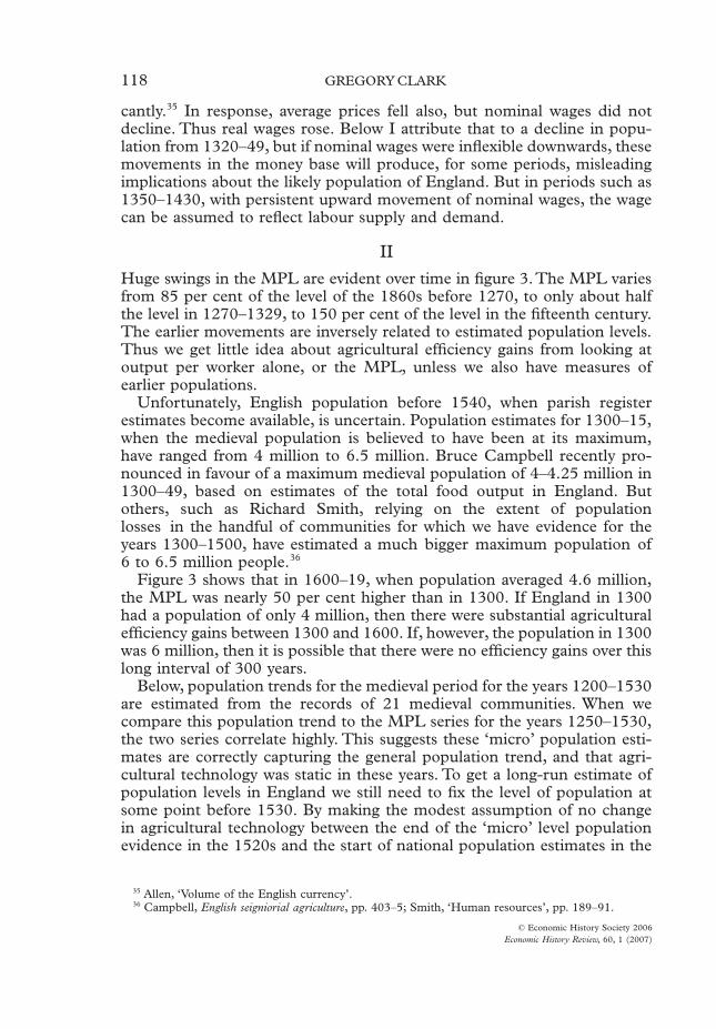
communities with population estimates in each decade and the total numberof persons reported.
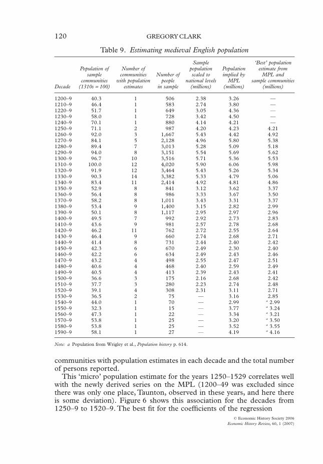
This ‘micro’ population estimate for the years 1250–1529 correlates wellwith the newly derived series on the MPL (1200–49 was excluded sincethere was only one place, Taunton, observed in these years, and here thereis some deviation). Figure 6 shows this association for the decades from1250–9 to 1520–9. The best fit for the coefficients of the regression
Table 9. Estimating medieval English population
Decade
Population ofsample
communities(1310s = 100)
Number ofcommunities
with populationestimates
Number ofpeople
in sample
Samplepopulationscaled to
national levels(millions)
Populationimplied by
MPL(millions)
‘Best’ populationestimate from
MPL andsample communities
(millions)
1200–9 40.3 1 506 2.38 3.26 —1210–9 46.4 1 583 2.74 3.80 —1220–9 51.7 1 649 3.05 4.36 —1230–9 58.0 1 728 3.42 4.50 —1240–9 70.1 1 880 4.14 4.21 —1250–9 71.1 2 987 4.20 4.23 4.211260–9 92.0 3 1,667 5.43 4.42 4.921270–9 84.1 5 2,128 4.96 5.80 5.381280–9 89.4 7 3,013 5.28 5.09 5.181290–9 94.0 8 3,151 5.54 5.69 5.621300–9 96.7 10 3,516 5.71 5.36 5.531310–9 100.0 12 4,020 5.90 6.06 5.981320–9 91.9 12 3,464 5.43 5.26 5.341330–9 90.3 14 3,382 5.33 4.79 5.061340–9 83.4 11 2,414 4.92 4.81 4.861350–9 52.9 8 841 3.12 3.62 3.371360–9 56.4 8 986 3.33 3.67 3.501370–9 58.2 8 1,011 3.43 3.31 3.371380–9 53.4 9 1,400 3.15 2.82 2.991390–9 50.1 8 1,117 2.95 2.97 2.961400–9 49.5 7 992 2.92 2.73 2.831410–9 43.6 9 981 2.57 2.78 2.681420–9 46.2 11 762 2.72 2.55 2.641430–9 46.4 9 660 2.74 2.68 2.711440–9 41.4 8 731 2.44 2.40 2.421450–9 42.3 6 670 2.49 2.30 2.401460–9 42.2 6 634 2.49 2.43 2.461470–9 43.2 4 498 2.55 2.47 2.511480–9 40.6 4 468 2.40 2.59 2.491490–9 40.5 4 413 2.39 2.43 2.411500–9 36.6 3 175 2.16 2.68 2.421510–9 37.7 3 280 2.23 2.74 2.481520–9 39.1 4 308 2.31 3.11 2.711530–9 36.5 2 75 — 3.16 2.851540–9 44.0 1 70 — 2.99 a 2.991550–9 32.3 1 15 — 3.77 a 3.241560–9 47.3 1 22 — 3.34 a 3.211570–9 53.8 1 25 — 3.20 a 3.501580–9 53.8 1 25 — 3.52 a 3.551590–9 58.1 1 27 — 4.19 a 4.16
Note: a Population from Wrigley et al., Population history p. 614.
THE LONG MARCH OF HISTORY 121
© Economic History Society 2006Economic History Review, 60, 1 (2007)
(7)
is
(8)
R2 = 0.93n = 28
where again the estimate is weighted, this time by the number of commu-nities involved in the the population estimates. There is no sign of anyupwards trend in MPL at a given population. Thus if we add a time trendto equation (7), T measured in decades from the 1250s, the estimatebecomes
(9)
The time trend is quantitatively and statistically insignificant. Thus, basedon the evidence of community trends, the agricultural technology of theyears 1250–1529 was static, with population alone determining MPL andoutput per worker.
ln lnMPL a b N et t t( ) = + ( ) +
ln . . ln
. .
MPL Nt t( ) = - ( )( ) ( )9 593 1 231
0 274 0 066
ln . . ln .
. . .
MPL N Tt t( ) = - ( ) -( ) ( ) ( )9 694 1 252 0 001
0 784 0 167 0 008
Figure 6. The marginal product of labour versus population, 1250–1529Note: The fitted curve uses a weighted regression, weighting on the number of people recorded in each decade.Source: Tabs. 1 and 9.
200
175
150
125
100
75
Mar
gina
l pro
duct
of
labo
ur
50
25
00 20 40 60
Sample population
1350s
1450s
1310s
80 100
120

122 GREGORY CLARK
© Economic History Society 2006Economic History Review, 60, 1 (2007)
This nice fit between the population trend estimated and the MPL doesnot prove that the population trend estimated is correct. But it does showthat these population estimates can provide a parsimonious explanation ofthe movements in the MPL over these years. Occam’s Razor tells us toprefer simple explanations over complex ones, and here we see a simple fitbetween two completely independently derived series.
A very similar association between population and the marginal productof labour is also found from the 1540s to 1610s, years when the parishrecords first yield national population estimates. Estimating the coefficientsof equation (7) for the decades from the 1540s to the 1610s, now measuringpopulation, Nt, in millions, we get as the best fit
(10)
R2 = 0.82n = 8
Note that the estimated proportionate effect of population on the marginalproduct of labour, measured by the coefficient on ln(Nt), is very similar tothe previous estimate. It suggests that again in 1540–1619 agriculturalefficiency was static.
The correlation between population and the marginal product of labourin both periods suggests that we can use the MPL in farming as a way offixing the average level of the population before 1530. Because the ‘micro’estimates of population trends in the medieval period and the nationalestimates do not overlap, the assumption that is crucial to this estimate isthat the efficiency of production in English agriculture was unchanged fromthe 1520s to the 1540s. This does not seem a particularly strong assumption.
To estimate national population levels before 1540 in millions with theaid of the marginal product of labour in agriculture, we can first estimatethe coefficients of the regression
(11)
for the decades of the 1250s to the 1520s, and the 1540s to the 1610s,where IND1250–1529 is 1 for the decades from the 1250s to the 1520s, and 0otherwise. Population, here the dependent variable, is measured as an indexbefore 1530, and in millions after that. The coefficient b in the regressionis a scaling factor that converts the population before 1530, measured as anindex, into millions. The connection between shifts in the marginal productof labour and population changes is assumed to be the same throughoutthe years before 1600. The fitted values for this regression are
(12)
R2 = 0.996n = 36
ln . . ln
. .
MPL Nt t( ) = - ( )( ) ( )5 908 1 078
0 274 0 209
ln lnN a bIND c MPL et t t( ) = + + ( ) +-1250 1529
ln . . . ln
. . .
N IND MPLt t( ) = + - ( )( ) ( ) ( )
-4 703 2 830 0 755
0 178 0 030 0 0391250 1529

THE LONG MARCH OF HISTORY 123
© Economic History Society 2006Economic History Review, 60, 1 (2007)
If the estimate is done allowing a different coefficient on the log of popu-lation from the 1540s to 1610s, the two coefficients do not differ quantita-tively or statistically.41
Column 5 of table 9 shows the national population totals implied by thesample of medieval communities with population estimates using this scal-ing procedure. We can also estimate the population in each decade beforethe 1540s from the marginal product of labour in agriculture using thecoefficients of the above expression. These estimates are shown in table 9,column 6. The final column of the table shows a ‘best’ estimate of popula-tion for the decades before 1540, which is just the average of the estimatesfrom the sample of communities and from the MPL.
Figure 7 shows this ‘best’ estimate, as well as the underlying estimatesfrom the sample communities, and from the marginal product of labour.All this suggests that with a very small amount of interpolation we caninterpret the years before 1600 as being ones where the technology wasstatic and the MPL was determined solely by population. In the decadesbefore 1240 there is a deviation between the direct population trend andthe MPL trend. This might be either technological advance in these years,or just problems with the data since the population trend in these years isbased on estimated population in one town only (Taunton), and the MPLdata is weakest here also.
On the ‘best’ estimate, population is estimated to have peaked just below6.0 million in the years 1310–16, just before the Great Famine of 1316–17.
41 This regression was again fitted weighting the earlier observations by the number of people in thepopulation.
Figure 7. Estimated medieval English populationSource: Tab. 9.
7
6
5
4
3
2
1N - community estimates N - ‘best estimate’
N - Wrigley et al
Onset ofPlague
N - MPL
0
Est
imat
ed p
opul
atio
n (m
illio
ns)
1200
1300
1400
1500
1600

124 GREGORY CLARK
© Economic History Society 2006Economic History Review, 60, 1 (2007)
The low point of population was in 1440–1520, when it is estimatedat 2.45 million.42 The famine of 1316–17 is estimated to have reducedpopulation by 11 per cent. The onset of the Black Death in 1348–9 is impliedto have carried away 31 per cent of the population. It is interesting to notethat in the two decades after the plague, at the time when there is someindication wages may have been underreported, the population estimatedfrom wages is larger than that estimated from the sample communities.
A high for pre-plague population of as much as 6 million has been rejectedby Campbell and others on the grounds that agriculture then had insuffi-cient yields to have supported this number of people.43 However, a closereading of the Campbell argument shows that it is based on one assumptionfor which there is very little support—that is that the total arable acreage inEngland c.1300 must have been at maximum 10.5 million acres, comparedto a total cultivated area in England in the 1880s of 26.5 million acres.44
Yet the Inquisitions Post Mortem suggest income from arable land was fully61 per cent of all landlords’ income.45 Given that meadow, pasture, andeven woodland, on average had a higher assessed value per acre than arable,this implies that the total cultivated area in England in 1300 was less than17.3 million acres. What was preventing the use for agriculture of the9.2 million acres later cultivated?
Some undoubtedly lay as waste, undrained, unreclaimed, and with min-imal output. Some lay in unimproved forest or Royal Forests. But thesefactors will not account for more than 10 to 20 per cent of land in cultivationin the 1880s. The amount of land that lay as common waste in England asearly as 1600 was extremely small, being definitely less than 5 per cent ofthe area of cultivated land in the nineteenth century.46 Most of this land layat sea level, or at altitudes greater than 250 metres. Given the absence ofpopulation pressures on land for most of the period 1350–1600, the extentof waste enclosure between 1300 and 1600 was presumably small. Wildforest lands, as opposed to the managed forest counted in the InquisitionsPost Mortem, in 1300 must have accounted for much less than 10 per centof the area later cultivated. So overall, it is hard to imagine more than4 million of acres in England in 1300 being waste, unimproved forest, orRoyal Forest, leaving at least 5.2 million acres unaccounted for under theCampbell story.
If that land was actually in use and cultivated in 1300, so that thecultivated area in 1300 was 85 per cent of that in the 1880s, then withCampbell’s estimates of grain output per acre and consumption per personthere would be a grain supply in 1300 to feed 5.75 million people, which
42 Since the Great Famine of 1316–17 produced a likely sharp decline in population, I use the years1310–16 before the famine for the 1310s, and 1318–29 after the famine for the 1320s.
43 Campbell, English seigniorial agriculture, pp. 386–410.44 Ibid., pp. 289–90. Wrigley, ‘Transition’, adopts this assumption from Campbell.45 Campbell, English seigniorial agriculture, pp. 66.46 Clark and Clark, ‘Common rights’.
THE LONG MARCH OF HISTORY 125
© Economic History Society 2006Economic History Review, 60, 1 (2007)
is the population estimated above for England around 1300 in table 9 above.Thus the MPL estimates above provide estimates of output per worker andof population totals, which are both feasible given what we know of medievalyields and land resources.
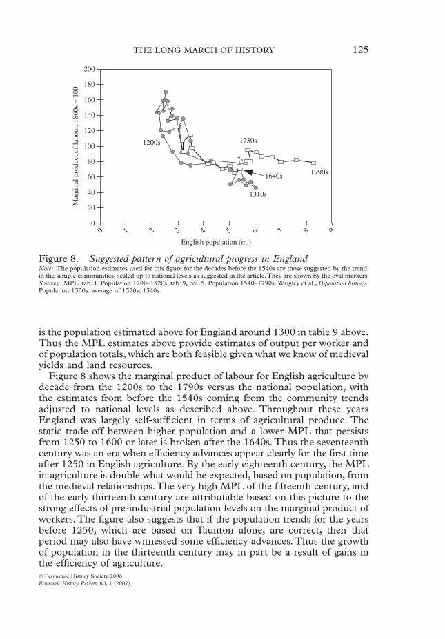
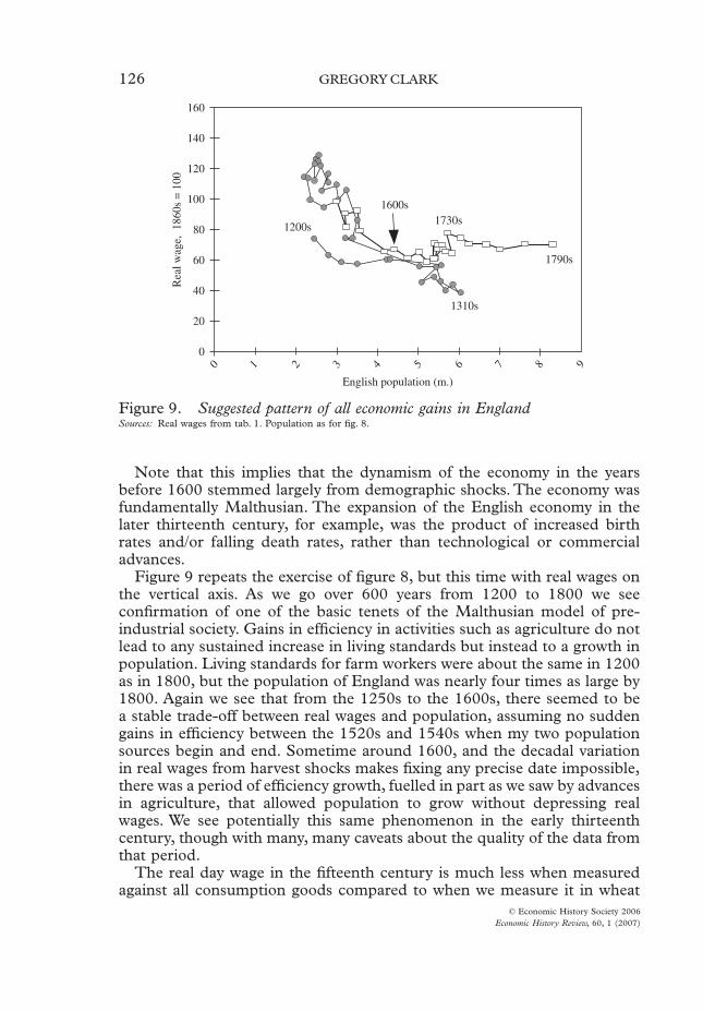
Figure 8 shows the marginal product of labour for English agriculture bydecade from the 1200s to the 1790s versus the national population, withthe estimates from before the 1540s coming from the community trendsadjusted to national levels as described above. Throughout these yearsEngland was largely self-sufficient in terms of agricultural produce. Thestatic trade-off between higher population and a lower MPL that persistsfrom 1250 to 1600 or later is broken after the 1640s. Thus the seventeenthcentury was an era when efficiency advances appear clearly for the first timeafter 1250 in English agriculture. By the early eighteenth century, the MPLin agriculture is double what would be expected, based on population, fromthe medieval relationships. The very high MPL of the fifteenth century, andof the early thirteenth century are attributable based on this picture to thestrong effects of pre-industrial population levels on the marginal product ofworkers. The figure also suggests that if the population trends for the yearsbefore 1250, which are based on Taunton alone, are correct, then thatperiod may also have witnessed some efficiency advances. Thus the growthof population in the thirteenth century may in part be a result of gains inthe efficiency of agriculture.
Figure 8. Suggested pattern of agricultural progress in EnglandNote: The population estimates used for this figure for the decades before the 1540s are those suggested by the trend in the sample communities, scaled up to national levels as suggested in the article. They are shown by the oval markers.Sources: MPL: tab. 1. Population 1200–1520s: tab. 9, col. 5. Population 1540–1790s: Wrigley et al., Population history. Population 1530s: average of 1520s, 1540s.
Mar
gina
l pro
duct
of
labo
ur, 1
860s
= 1
00
0
20
40
60
80
100
120
140
160
180
200
9876
1310s
1790s1640s
1730s1200s
54
English population (m.)
3210
126 GREGORY CLARK
© Economic History Society 2006Economic History Review, 60, 1 (2007)
Note that this implies that the dynamism of the economy in the yearsbefore 1600 stemmed largely from demographic shocks. The economy wasfundamentally Malthusian. The expansion of the English economy in thelater thirteenth century, for example, was the product of increased birthrates and/or falling death rates, rather than technological or commercialadvances.
Figure 9 repeats the exercise of figure 8, but this time with real wages onthe vertical axis. As we go over 600 years from 1200 to 1800 we seeconfirmation of one of the basic tenets of the Malthusian model of pre-industrial society. Gains in efficiency in activities such as agriculture do notlead to any sustained increase in living standards but instead to a growth inpopulation. Living standards for farm workers were about the same in 1200as in 1800, but the population of England was nearly four times as large by1800. Again we see that from the 1250s to the 1600s, there seemed to bea stable trade-off between real wages and population, assuming no suddengains in efficiency between the 1520s and 1540s when my two populationsources begin and end. Sometime around 1600, and the decadal variationin real wages from harvest shocks makes fixing any precise date impossible,there was a period of efficiency growth, fuelled in part as we saw by advancesin agriculture, that allowed population to grow without depressing realwages. We see potentially this same phenomenon in the early thirteenthcentury, though with many, many caveats about the quality of the data fromthat period.
The real day wage in the fifteenth century is much less when measuredagainst all consumption goods compared to when we measure it in wheat
Figure 9. Suggested pattern of all economic gains in EnglandSources: Real wages from tab. 1. Population as for fig. 8.
Rea
l wag
e, 1
860s
= 1
00
98765
English population (m.)
432100
20
40
60
1200s
1600s1730s
1310s
1790s
80
100
120
140
160

THE LONG MARCH OF HISTORY 127
© Economic History Society 2006Economic History Review, 60, 1 (2007)
only, or even in all agricultural output. But it still was about 15 per centabove the farm day wages of the 1860s at the end of the Industrial Revolution.Thus under the right conditions material living standards in pre-industrialEurope could be very high. The Malthusian world was not necessarily onewhere people were pressed to the limits of physical subsistence.
III
This article shows, that using day wages, we can build a picture of Englishagricultural history that presents an internally consistent picture of the realwage, the MPL, output per farm worker, national population, the shareemployed in agriculture, and agricultural efficiency in general, from 1200to 1869. The only major feature of early England that this picture cannotincorporate is the low urbanization share. But as noted, Dyer argues thislow apparent urbanization share may stem from England having a town-sizedistribution unusually weighted towards small towns. The picture is one ofa static agricultural technology before 1600, but a technology that producedrelatively high output per worker even in 1300, and that supporting asubstantial population in the years before 1349.
University of California, Davis
Date submitted 8 March 2005Revised version submitted 24 August 2005Accepted 3 December 2005
DOI: 10.1111/j.1468-0289.2006.00358.x
Footnote referencesAllen, M. R., ‘The volume of the English currency, 1158–1470’, Economic History Review, 2nd ser., LIV
(2001), pp. 595–611.Allen, R. C., ‘Economic structure and agricultural productivity in Europe, 1300–1800’, European Review
of Economic History, 3 (2000), pp. 1–25.Bennett, J. M., Women in the medieval English countryside: gender and household in Brigstock before the plague
(1987).Beveridge, W., ‘Wages in the Winchester manors’, Economic History Review, VII (1936), pp. 22–43.Beveridge, W., Prices and wages in England, vol. 1: the Mercantilist era (1939).Blanchard, I. S. W., The middle ages: a concept too many? (1996).Bowden, P. J., ‘Statistical appendix’, in Joan Thirsk, ed., The agrarian history of England and Wales,
Vol. IV (1967), pp. 814–70.Bowden, P. J., ‘Statistical appendix’, in Joan Thirsk, ed., The agrarian history of England and Wales,
Vol. V.II (1985), pp. 827–902.Britton, E., The community of the vill (1977).Campbell, B. M. S., English seigniorial agriculture, 1250–1450 (2000).Clark, G., ‘Labour productivity in English agriculture, 1300–1860’, in B. M. S. Campbell, and
M. Overton, eds., Agricultural productivity in the European past (1991), pp. 211–35.Clark, G., ‘Yields per acre in English agriculture 1266–1860: evidence from payments to labour’,
Economic History Review 2nd ser. XLIV (1991), pp. 445–60.Clark, G., ‘Farm wages and living standards in the industrial revolution: England, 1670–1850’, Economic
History Review, 2nd ser. LIV (2001), pp. 477–505.

128 GREGORY CLARK
© Economic History Society 2006Economic History Review, 60, 1 (2007)
Clark, G., ‘The agricultural revolution and the industrial revolution, 1500–1912’, Working paper, Universityof California, Davis (2002).
Clark, G., ‘The price history of English agriculture, 1209–1914’, Research in Economic History, 22(2004), pp. 41–120.
Clark, G., ‘The condition of the working-class in England, 1209–2004’, Journal of Political Economy,113 (2005) 1307–40.
Clark, G. and Clark, A., ‘Common rights in land in England, 1475–1839’, Journal of Economic History,LXI (2001), pp. 1009–36.
Davenport, F. G., The economic development of a Norfolk manor, 1086–1565 (1906).DeWindt, E. B., Land and people in Holywell-cum-Needingworth (1972).Dyer, C. C., Everyday life in medieval England (1994).Farmer, D. L., ‘Prices and wages’, in H. E. Hallam, ed., The agrarian history of England and Wales, vol.
II, 1042–1350 (1988), pp. 716–817.Farmer, D. L., ‘Prices and wages, 1350–1500’, in E. Miller, ed., The agrarian history of England and
Wales, vol. III, 1348–1500 (1991), pp. 431–525.Gottfried, R. S., The Black Death: natural and human disaster in medieval Europe (1983).Hatcher, J., Plague, population, and the English economy, 1348–1530 (1977).Horrell, S., ‘Home demand and British industrialization’, Journal of Economic History, 56 (1996),
pp. 561–604.Karakacili, E., ‘English agrarian labour productivity rates before the Black Death: a case study’, Journal
of Economic History, 64 (2004), pp. 24–60.Munro, J., ‘Postan, population, and prices in late-medieval England and Flanders’, Working paper, Depart-
ment of Economics, University of Toronto (2002).Munro, J., ‘Wage stickiness, monetary changes, and real incomes in late-medieval England and the Low
Countries: did money matter?’, Research in Economic History, 21 (2001), pp. 185–297.Poos, L. R., A rural society after the black Death: Essex, 1350–1525 (1991).Poos, L. R. and Smith, R. M., ‘ “Legal windows onto historical population?” Recent research
on demography and the manor court in medieval England,’ Law and History Review, 2 (1984),pp. 128–52.
Raftis, J. A., Warboys: two hundred years in the life of an English mediaeval village (1974).Raftis, J. A., A small town in late medieval England: Godmanchester, 1278–1400 (1982).Razi, Z., Life, marriage and death in a medieval parish: economy, society and demography in Halesowen,
1270–1400 (1980).Razi, Z., ‘The demographic transparency of manorial court rolls,’ Law and History Review, 5 (1987),
pp. 89–98.Razi, Z., ‘Manorial court rolls and local population: an East Anglian case study,’ Economic History
Review, 2nd ser., XLIX (1996), pp. 758–63.Shrewsbury, J. F. D., A history of bubonic plague in the British Isles (1970).Smith, R. M., ‘Human resources’, in G. Astill and A. Grant, eds., The countryside of medieval England
(1988).Titow, J. Z., ‘Some evidence of thirteenth-century population growth’, Economic History Review, 2nd ser.,
XIV (1961), pp. 218–23.Wrigley, E. A., ‘Urban growth and agricultural change: England and the Continent in the early modern
period’, Journal of Interdisciplinary History, 25 (1985), pp. 683–728.Wrigley, E. A., ‘The transition to an advanced organic economy: half a millennium of English agricul-
ture’, manuscript, Cambridge University (2005).Wrigley, E. A., Davies, R. S., Oeppen, J. E., and Schofield, R. S., English population history from family
reconstitution, 1580–1837 (1997).
THE LONG MARCH OF HISTORY 129
© Economic History Society 2006Economic History Review, 60, 1 (2007)
APPENDIX: Estimating day wages in a regression frameworkThe basic model of wages that was fitted to the data is
The dependent variable is the logarithm of wage payments. Nominal day wagesincreased by 15–20 fold over the years 1209–1869. By using the logarithm of wagesthe various controls on the right-hand side of the equation, such as for location,have the same proportional influence on wages across all years.
LOCi is an indicator variable, 1 when the observation is from parish i, 0 otherwise.t indexes the year. Dt is 1 in year t, 0 otherwise. DSEASj is an indicator for theseason of the year the wage payment comes from. In addition to the five basiccategories (winter, summer, hay, harvest, and unknown) an indicator was includedfor harvest wages drawn from counties where by 1866 70 per cent or more of landwas in arable cultivation. The harvest wage premium in such areas tended to bemuch greater. DTYPEk is a set of 21 indicator variables for the type of wagepayment. The first was a regular day wage, and the other 20 were for payments forthreshing different grains (such as wheat, rye, barley, and oats) or combinations ofgrains. The threshing payments are mainly those for threshing wheat, barley, andoats.
To allow for variations in the ratio of the payment for threshing a bushel of grainto the day wage over time, a set of 21 indicators DTHl was added. This allowed theratio of threshing payments to day wages to vary from that of the pre-plague years1209–1349, which was used as the base period. The other periods were each25-year interval starting in 1350, ending with the 26-year interval 1825–50. Some-times threshing payments were combined with those for winnowing the grain. Theindicator DWIN was set to 1 in these cases, 0 otherwise. To control for differencesin regional wage movements, a separate regional indicator was included for thenorth, midlands, and south west for the periods 1209–1499, 1500–99, 1600–99,1700–49, 1750–99, 1800–49, 1850–69. There were not sufficient observations offarm wages in the north before 1500 to estimate this indicator for 1209–1499.Instead the relative wages of building workers in the north versus the south east for1209–1499 were used to estimate this value. Clark, ‘Condition of the working class’describes how these wage estimates were derived.
Table A1 shows the estimated values of the more important control variables,their standard errors, and t-values. In the last column is shown the importance ofthe control in terms of its percentage effect on the wage level, where applicable.Table A2 records the estimated national day wage by year outside hay and harvest,once the raw series was adjusted.
ln Wage a LOC b D c DSEAS
d DTYPE f DTH gDWIN h DPER DREG e
it i i t t j jjti
k k l l mn m n itnmlk
( ) = + +
+ + + + +
ÂÂÂÂÂÂÂ

130 GREGORY CLARK
© Economic History Society 2006Economic History Review, 60, 1 (2007)
Table A1. The values of the control coefficients in the wage regression
VariableCoefficientestimate
Standarderror T-value
Percentageeffect
SUMMER 0.04 0.006 6.3** +4HARVEST—Pasture Ares 0.34 0.012 29.4** +41HARVEST—Grain Area 0.59 0.013 45.0** +81HAY 0.28 0.009 29.3** +32UNKNOWN SEASON 0.08 0.006 12.1** +8THRESH WHEAT (QU), 1209–1349 0.45 0.014 33.0 —THRESH RYE (QU), 1209–1349 0.41 0.016 26.4 —THRESH BARLEY (QU), 1209–1349 0.00 0.014 0.1 —THRESH OATS (QU), 1209–1349 −0.35 0.014 −25.3 —DWINNOW 0.11 0.008 14.0 11DTHRESH1350–1374 −0.28 0.020 −14.1 −24DTHRESH1375–1399 −0.32 0.021 −15.2 −27DTHRESH1400–1424 −0.35 0.020 −17.1 −30DTHRESH1425–1449 −0.35 0.024 −14.4 −30DTHRESH1450–1474 −0.38 0.034 −11.1 −32DTHRESH1475–1499 −0.41 0.065 −6.3 −34DTHRESH1500–1524 −0.29 0.052 −5.7 −25DTHRESH1525–1549 −0.11 0.042 −2.5 −10DTHRESH1550–1574 −0.04 0.041 −0.9 −4DTHRESH1575–1599 0.01 0.041 0.3 1DTHRESH1600–1624 0.02 0.033 0.7 2DTHRESH1625–1649 0.07 0.037 1.8 7DTHRESH1650–1674 0.25 0.030 8.3 29DTHRESH1675–1699 0.19 0.029 6.7 21DTHRESH1700–1724 0.18 0.027 6.8 20DTHRESH1725–1749 0.19 0.021 9.1 21DTHRESH1750–1774 0.21 0.023 9.1 23DTHRESH1775–1799 0.28 0.022 12.7 33DTHRESH1800–1824 0.24 0.020 12.2 27DTHRESH1825–1850 0.11 0.021 5.3 12
Notes: ** significantly different from 0 at the 1% level.* significantly different from 0 at the 5% level.
Table A2: Nominal and Real Wages by Year, 1209–1869
YearNominal
wageRealwage Year
Nominalwage
Realwage Year
Nominalwage
Realwage
1209 1.36 70 1430 3.69 101 1650 9.78 521210 1431 3.58 116 1651 10.45 601211 1.15 53 1432 3.60 126 1652 9.29 581212 1.18 60 1433 3.77 108 1653 9.81 661213 1434 3.61 117 1654 9.97 791214 1.41 73 1435 3.69 121 1655 9.38 751215 1436 3.66 116 1656 12.32 851216 1.25 59 1437 3.47 111 1657 9.13 591217 1438 4.10 99 1658 10.75 651218 1.13 49 1439 3.66 80 1659 9.29 531219 1.36 60 1440 3.77 106 1660 9.65 591220 1.20 58 1441 3.63 141 1661 9.04 521221 1.28 54 1442 3.59 133 1662 9.91 541222 1443 3.66 129 1663 11.28 71
THE LONG MARCH OF HISTORY 131
© Economic History Society 2006Economic History Review, 60, 1 (2007)
1223 1444 3.71 133 1664 13.39 841224 1.29 64 1445 3.64 138 1665 9.61 651225 1.25 50 1446 3.71 123 1666 11.49 811226 1.24 51 1447 3.54 111 1667 10.46 771227 1.12 46 1448 3.67 123 1668 10.17 741228 1449 3.70 121 1669 9.48 651229 1450 3.74 122 1670 9.97 681230 1451 4.36 135 1671 9.75 671231 1452 3.87 124 1672 9.83 701232 1.13 49 1453 3.69 117 1673 9.92 661233 1.19 54 1454 3.86 128 1674 9.54 561234 1455 3.71 133 1675 10.10 621235 1456 3.69 129 1676 10.22 741236 1.15 56 1457 3.76 132 1677 9.33 641237 1.18 52 1458 3.78 121 1678 9.93 651238 1459 4.12 127 1679 9.24 601239 1460 3.58 111 1680 9.82 671240 1461 3.64 104 1681 10.44 681241 1462 3.75 109 1682 9.58 641242 1463 3.58 135 1683 9.86 671243 1464 3.70 145 1684 9.83 651244 1465 3.73 140 1685 9.88 621245 1.17 61 1466 3.66 131 1686 10.99 781246 1.24 57 1467 3.43 117 1687 8.77 641247 1.24 48 1468 3.58 116 1688 9.50 731248 1.22 1469 3.48 114 1689 10.17 801249 1.27 56 1470 3.59 114 1690 9.42 711250 1.13 1471 3.18 97 1691 9.42 721251 1.48 66 1472 4.25 139 1692 9.82 641252 1.25 54 1473 3.34 117 1693 9.36 551253 1.26 50 1474 3.78 139 1694 10.05 601254 1.32 66 1475 1695 9.41 601255 1.28 61 1476 1696 9.89 561256 1477 4.05 137 1697 9.19 521257 1.31 49 1478 3.34 105 1698 9.57 511258 1.26 45 1479 3.12 96 1699 9.64 551259 1480 3.06 101 1700 9.56 611260 1481 3.27 106 1701 9.66 681261 1.32 1482 3.26 91 1702 10.06 721262 1.73 70 1483 4.77 124 1703 10.06 761263 1.28 51 1484 3.65 106 1704 9.85 681264 1.17 47 1485 3.94 132 1705 9.52 711265 1.26 51 1486 3.66 123 1706 9.87 741266 1.22 50 1487 4.22 137 1707 9.80 741267 1488 2.95 98 1708 10.03 691268 1.23 53 1489 2.92 93 1709 9.23 511269 1.26 48 1490 2.76 88 1710 9.29 491270 1.20 45 1491 2.51 78 1711 9.76 581271 1.24 42 1492 5.40 174 1712 9.78 631272 1.21 40 1493 1713 9.72 621273 1.28 48 1494 3.86 133 1714 10.16 621274 1.29 44 1495 3.57 131 1715 10.20 701275 1.29 42 1496 3.68 138 1716 10.13 661276 1.34 47 1497 3.24 100 1717 10.49 691277 1.24 40 1498 3.69 122 1718 10.23 71
YearNominal
wageRealwage Year
Nominalwage
Realwage Year
Nominalwage
Realwage
Table A2. Continued
132 GREGORY CLARK
© Economic History Society 2006Economic History Review, 60, 1 (2007)
1278 1.22 45 1499 3.96 125 1719 9.75 701279 1.30 50 1500 3.19 113 1720 10.11 661280 1.40 47 1501 3.36 99 1721 9.83 671281 1.36 50 1502 3.30 94 1722 9.38 661282 1.32 43 1503 3.82 118 1723 10.50 731283 1.31 43 1504 3.33 103 1724 9.56 661284 1.44 49 1505 3.07 100 1725 9.23 591285 1.37 56 1506 3.38 114 1726 9.63 601286 1.28 47 1507 3.38 112 1727 9.97 641287 1.32 54 1508 3.33 109 1728 9.85 551288 1.27 65 1509 3.26 133 1729 9.98 581289 1.24 57 1510 3.44 133 1730 10.67 721290 1.26 46 1511 3.44 127 1731 10.66 771291 1.38 44 1512 3.39 109 1732 10.50 821292 1.33 46 1513 3.00 82 1733 10.87 831293 1.29 43 1514 3.24 100 1734 10.50 741294 1.35 39 1515 3.03 95 1735 10.73 721295 1.32 36 1516 3.59 105 1736 10.94 741296 1.29 37 1517 3.17 109 1737 10.88 761297 1.28 45 1518 3.37 100 1738 10.87 781298 1.28 40 1519 3.51 102 1739 10.72 751299 1.30 41 1520 4.14 110 1740 10.15 611300 1.40 44 1521 3.70 91 1741 10.45 611301 1.38 46 1522 3.51 97 1742 10.55 721302 1.34 46 1523 3.70 104 1743 10.43 791303 1.32 48 1524 3.82 108 1744 10.37 821304 1.39 54 1525 3.01 92 1745 10.45 791305 1.35 45 1526 3.10 100 1746 10.63 741306 1.25 43 1527 3.03 87 1747 10.51 751307 1.24 44 1528 3.35 65 1748 10.92 751308 1.31 43 1529 3.22 81 1749 10.92 751309 1.28 37 1530 4.21 102 1750 10.67 741310 1.41 36 1531 3.60 87 1751 10.63 711311 1.33 35 1532 3.22 78 1752 10.80 691312 1.33 43 1533 3.61 85 1753 10.77 701313 1.35 44 1534 4.23 116 1754 10.93 721314 1.35 42 1535 2.89 71 1755 10.98 751315 1.37 39 1536 2.23 54 1756 10.45 661316 1.47 29 1537 4.19 102 1757 11.01 591317 1.60 32 1538 3.51 95 1758 10.97 641318 1.54 42 1539 3.34 91 1759 11.01 731319 1.43 53 1540 4.01 108 1760 11.47 801320 1.61 52 1541 4.36 108 1761 11.25 771321 1.51 44 1542 4.20 109 1762 11.20 721322 1.62 35 1543 4.04 100 1763 11.09 681323 1.48 36 1544 4.11 95 1764 11.03 661324 1.49 43 1545 3.61 72 1765 11.34 651325 1.52 41 1546 3.88 69 1766 11.53 661326 1.45 46 1547 4.24 104 1767 12.86 671327 1.44 53 1548 4.00 97 1768 11.47 621328 1.56 51 1549 4.14 81 1769 11.45 681329 1.51 44 1550 5.46 82 1770 11.53 691330 1.53 44 1551 4.72 66 1771 12.03 651331 1.45 38 1552 5.27 82 1772 12.07 621332 1.50 41 1553 5.20 93 1773 11.71 60
YearNominal
wageRealwage Year
Nominalwage
Realwage Year
Nominalwage
Realwage
Table A2. Continued
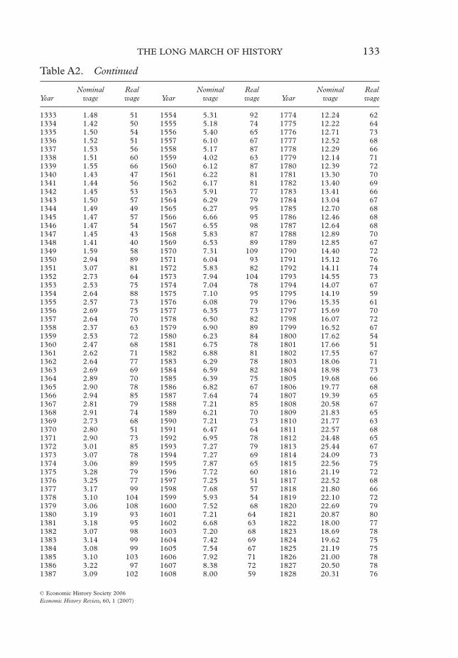
THE LONG MARCH OF HISTORY 133
© Economic History Society 2006Economic History Review, 60, 1 (2007)
1333 1.48 51 1554 5.31 92 1774 12.24 621334 1.42 50 1555 5.18 74 1775 12.22 641335 1.50 54 1556 5.40 65 1776 12.71 731336 1.52 51 1557 6.10 67 1777 12.52 681337 1.53 56 1558 5.17 87 1778 12.29 661338 1.51 60 1559 4.02 63 1779 12.14 711339 1.55 66 1560 6.12 87 1780 12.39 721340 1.43 47 1561 6.22 81 1781 13.30 701341 1.44 56 1562 6.17 81 1782 13.40 691342 1.45 53 1563 5.91 77 1783 13.41 661343 1.50 57 1564 6.29 79 1784 13.04 671344 1.49 49 1565 6.27 95 1785 12.70 681345 1.47 57 1566 6.66 95 1786 12.46 681346 1.47 54 1567 6.55 98 1787 12.64 681347 1.45 43 1568 5.83 87 1788 12.89 701348 1.41 40 1569 6.53 89 1789 12.85 671349 1.59 58 1570 7.31 109 1790 14.40 721350 2.94 89 1571 6.04 93 1791 15.12 761351 3.07 81 1572 5.83 82 1792 14.11 741352 2.73 64 1573 7.94 104 1793 14.55 731353 2.53 75 1574 7.04 78 1794 14.07 671354 2.64 88 1575 7.10 95 1795 14.19 591355 2.57 73 1576 6.08 79 1796 15.35 611356 2.69 75 1577 6.35 73 1797 15.69 701357 2.64 70 1578 6.50 82 1798 16.07 721358 2.37 63 1579 6.90 89 1799 16.52 671359 2.53 72 1580 6.23 84 1800 17.62 541360 2.47 68 1581 6.75 78 1801 17.66 511361 2.62 71 1582 6.88 81 1802 17.55 671362 2.64 77 1583 6.29 78 1803 18.06 711363 2.69 69 1584 6.59 82 1804 18.98 731364 2.89 70 1585 6.39 75 1805 19.68 661365 2.90 78 1586 6.82 67 1806 19.77 681366 2.94 85 1587 7.64 74 1807 19.39 651367 2.81 79 1588 7.21 85 1808 20.58 671368 2.91 74 1589 6.21 70 1809 21.83 651369 2.73 68 1590 7.21 73 1810 21.77 631370 2.80 51 1591 6.47 64 1811 22.57 681371 2.90 73 1592 6.95 78 1812 24.48 651372 3.01 85 1593 7.27 79 1813 25.44 671373 3.07 78 1594 7.27 69 1814 24.09 731374 3.06 89 1595 7.87 65 1815 22.56 751375 3.28 79 1596 7.72 60 1816 21.19 721376 3.25 77 1597 7.25 51 1817 22.52 681377 3.17 99 1598 7.68 57 1818 21.80 661378 3.10 104 1599 5.93 54 1819 22.10 721379 3.06 108 1600 7.52 68 1820 22.69 791380 3.19 93 1601 7.21 64 1821 20.87 801381 3.18 95 1602 6.68 63 1822 18.00 771382 3.07 98 1603 7.20 68 1823 18.69 781383 3.14 99 1604 7.42 69 1824 19.62 751384 3.08 99 1605 7.54 67 1825 21.19 751385 3.10 103 1606 7.92 71 1826 21.00 781386 3.22 97 1607 8.38 72 1827 20.50 781387 3.09 102 1608 8.00 59 1828 20.31 76
YearNominal
wageRealwage Year
Nominalwage
Realwage Year
Nominalwage
Realwage
Table A2. Continued

134 GREGORY CLARK
© Economic History Society 2006Economic History Review, 60, 1 (2007)
Sources of the farm wage database47
Barmby, James. Memorials of St Gile’s, Durham. Publications of the Surtees Society, Vol. 95 (1896).Bedford Record Office. Chester, 938. Boteler, TW 800, 802, 805, 809.Berkshire Record Office. Buscot, D/ELV E68.Beveridge Collection, Robbins Library, London School of Economics. Battle Abbey (Boxes H6, H8, W4),
Brooke, Isle of Wight (I11), Croyland (Oakington) (W4), Delisle Accounts (W2), Eton (I19), Exeter
1388 3.18 114 1609 6.89 50 1829 20.59 801389 2.97 112 1610 8.22 67 1830 20.02 771390 2.91 86 1611 8.37 67 1831 21.30 821391 3.13 79 1612 7.90 60 1832 20.87 871392 2.59 82 1613 7.26 52 1833 20.43 881393 2.92 109 1614 8.33 61 1834 19.69 881394 2.79 98 1615 7.14 53 1835 19.08 891395 3.01 104 1616 7.76 57 1836 19.30 841396 3.08 106 1617 8.16 59 1837 20.19 821397 3.21 91 1618 7.86 58 1838 20.39 811398 2.95 87 1619 8.05 64 1839 21.20 771399 3.42 106 1620 7.77 66 1840 21.51 811400 3.40 102 1621 7.99 66 1841 21.65 841401 3.47 98 1622 7.54 53 1842 21.48 891402 3.50 88 1623 8.20 59 1843 20.55 961403 3.50 101 1624 7.49 56 1844 20.76 941404 3.53 118 1625 8.25 61 1845 20.83 931405 3.41 117 1626 8.62 62 1846 21.07 881406 3.46 126 1627 8.36 66 1847 21.89 801407 3.50 121 1628 8.84 70 1848 21.43 951408 3.53 107 1629 8.82 68 1849 20.50 951409 3.44 97 1630 8.14 53 1850 18.91 941410 3.54 87 1631 8.91 54 1851 19.03 981411 3.49 100 1632 8.41 56 1852 19.59 1001412 3.49 112 1633 8.83 61 1853 20.88 931413 3.49 116 1634 8.39 59 1854 23.45 941414 3.58 121 1635 8.77 59 1855 23.89 911415 3.61 119 1636 9.84 66 1856 24.31 951416 3.39 95 1637 8.54 56 1857 23.40 961417 3.44 90 1638 8.90 54 1858 22.89 1041418 3.32 98 1639 9.25 63 1859 23.76 1091419 3.59 104 1640 9.24 68 1860 21.97 911420 3.12 102 1641 9.52 64 1861 22.68 941421 3.53 107 1642 9.55 70 1862 23.36 971422 3.41 112 1643 9.14 64 1863 22.49 1021423 3.34 118 1644 8.79 61 1864 22.30 1061424 3.70 127 1645 8.73 61 1865 22.68 1041425 3.65 117 1646 8.90 59 1866 23.96 1001426 3.64 122 1647 9.80 56 1867 25.04 981427 3.49 120 1648 9.56 49 1868 25.73 1021428 3.69 129 1649 9.30 49 1869 24.72 1061429 3.52 95
47 To save space only references to manuscript sources not found in Clark, ‘Farm wages’, are givenhere.
YearNominal
wageRealwage Year
Nominalwage
Realwage Year
Nominalwage
Realwage
Table A2. Continued
THE LONG MARCH OF HISTORY 135
© Economic History Society 2006Economic History Review, 60, 1 (2007)
Accounts (W5), Hinderclay (G14), Pelham Papers (H12), Penshurst (W2, W7), Stowe Papers (H2),St Bartholomew’s Hospital, Sandwich (E9), Trinity College, Cambridge (W2), Winchester College(W2), Westminster Abbey (P9–10, X10).
Buckingham Record Office. Chester, D/C/4/5.Cumbria Record Office (Carlisle). Curwen, D/LONS. Pennington D/PENN/202.Essex Record Office. Petre, D/DP/A18–21, A47, A54–55.Farmer Collection, Library, University of Saskatchewan. Winchester (Ashmansworth, Downton,
Ebbesbourne, Farnham, Harwell, High Clere, Ivinghoe, Meon, Meon Church, Overton, Witney, WestWycombe, Wolvesey, Woodhay), Westminster (Ashford, Birdbrook, Eybury, Halliford, Hyde, Islip,Knightsbridge, Oakham), Queen’s College (Gussage, Werrore and Corsham), Bircham, Claret, Deer-hurst, Farley, Hinderclay, Maldon, Pershore, Redgrave, III.B.45, III.B.48.
Fussell, G. E., ed., Robert Loder’s farm accounts, 1610–1620 (Camden Third Ser., 53, 1936).Gloucester Record Office. D 1571/A12–A45.Hampshire Record Office. Shipway, 2M37/341, 343.Harland, J., ed., The house and farm accounts of the Shuttleworths of Gawthorpe Hall. Parts 1 and 2.
Chetham Society, 35 and 41 (1956).Hertford Record Office. Radcliffe, D/ER E97, E110, E115.Kent Record Office. Sackville, U269/A49/2–3, U269/A60–1. Tylden, U593/A7, A10.Lodge, Eleanor. 1927. The Account Book of a Kentish Estate, 1616–1704. London: British Academy,
Records of Social and Economic History, Vol. 6.Norfolk Record Office. Lukin, WKC 5/229, 233, 250. Stimpson, MC 561/44, 49. Tompson, MC 561/42,
47.Northampton Record Office. Dryden, D(CA) 305. Fitzwilliam Misc. Vol. 189.Northumberland Record Office (Newcastle). Swinburne, ZSW, 227, 228/2.Nottinghamshire Record Office. Cullen, DD 1571/11. Dunston, DDN 213/5–7, 11–13. Ward, DDSJ 36.
Webb Edge, DDE 1/5, 12, DDE 3/24, DDE 28/2.Owen, A. E. B., The Medieval Lindsey Marsh: Select Documents. Lincoln Record Society Publications,
Vol. 85 (1996).Postles, D., Stubbington Manorial Accounts (manuscript) (2003).Reading University Library. GLO 1/2/1. Micro. P262. SAL 5/1/1. Buckingham, BUC 11/1/11. Pyrford
Green Farm. SUR 2/1/1.Records of the Borough of Nottingham. 1885 1889. Vol III (1485–1547), Vol. IV (1547–1625).Ritchie, N., ‘Labour Conditions in Essex in the Reign of Richard II’, Econ. Hist. Rev., 4 (1934).Thorold Rogers, J. E., A history of agriculture and prices in England: vol. 2 (1866).Thorold Rogers, J. E., A history of agriculture and prices in England: vol. 3 (1888).Thorold Rogers, J. E., A history of agriculture and prices in England: vol. 6 (1888).Shropshire Record Office. Apley Park. 5586/5/17/22–36.Somerset Record Office. Dunster Castle. DD/L 1/5/16–17.Surrey Record Office (Guildford). More-Molyneux, LM 1087/1/8.Yorkshire Record Office (Sheepscar). Robinson/Weddell, NH 2187.
Vol. 60, N
o. 1T
HE
EC
ON
OM
IC H
ISTO
RY
RE
VIE
WFebruary 2007
CONTENTS
ARTICLESGLEN O’HARA
Towards a new Bradshaw? Economic statistics and the British state in the 1950s and 1960s
E. A. WRIGLEYEnglish county populations in the later eighteenth century
GRAHAM BROWNLOWThe causes and consequences of rent-seeking in Northern Ireland,
1945–72
GREGORY CLARKThe long march of history: Farm wages, population, and economic
growth, England 1209–1869
REVIEW OF PERIODICAL LITERATUREDAVID PRATT, P. R. SCHOFIELD, HENRY FRENCH, PETER KIRBY,
MARK FREEMAN AND JULIAN GREAVES, AND HUGH PEMBERTON
BOOK REVIEWS
This journal is available online at BlackwellSynergy. Visit www.blackwell-synergy.com tosearch the articles and register for table ofcontents e-mail alerts.
VOLUME 60, NO. 1 FEBRUARY 2007
0013-0117(200702)60:1;1-I