olivier blanchard may 12, 2007 - mit opencourseware · olivier blanchard may 12, 2007 nr. 1 cite...

14.452. Topic 9. Monetary policy. Notes.

Olivier Blanchard

May 12, 2007

Nr. 1 Cite as: Olivier Blanchard, course materials for 14.452 Macroeconomic Theory II, Spring 2007. MIT OpenCourseWare (http://ocw.mit.edu/), Massachusetts Institute of Technology. Downloaded on [DD Month YYYY].

Look at three issues:

Time consistency. The inflation bias. •

The trade-off between inflation and activity. •

Implementation and Taylor rules. •

Other issues, not touched:

Disinflation. Optimal speed. •

Liquidity traps. The non negativity constraint for interest rates.•

Exchange rates. Should they matter only through their effect on activity • and inflation?


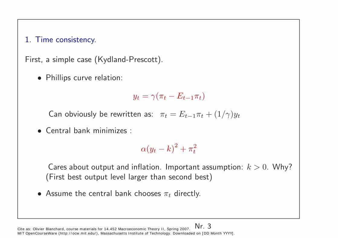
1. Time consistency.

First, a simple case (Kydland-Prescott).

Phillips curve relation: •

yt = γ(πt − Et−1πt)

Can obviously be rewritten as: πt = Et−1πt + (1/γ)yt

Central bank minimizes :•

α(yt − k)2 + πt 2

Cares about output and inflation. Important assumption: k > 0. Why? (First best output level larger than second best)

• Assume the central bank chooses πt directly.


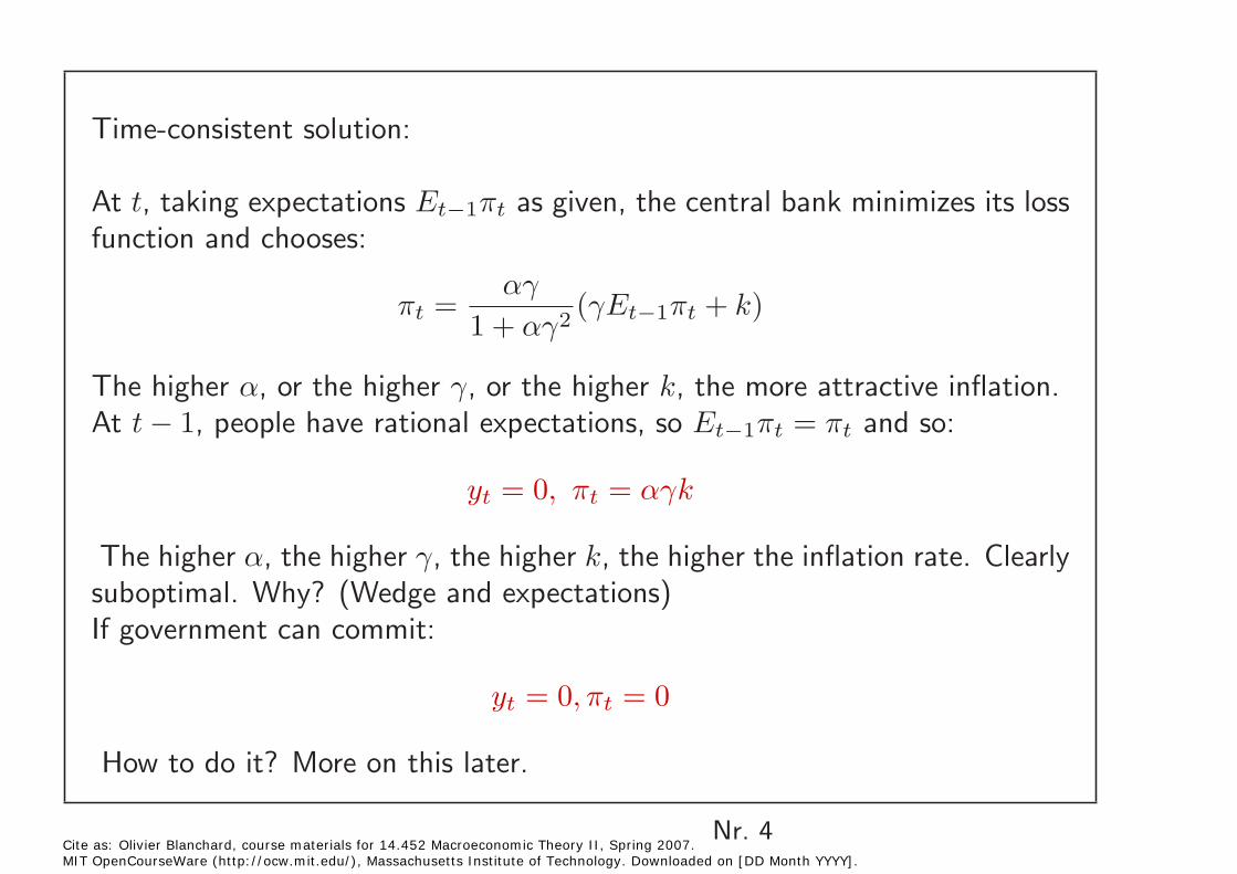
Time-consistent solution:

At t, taking expectations Et−1πt as given, the central bank minimizes its loss function and chooses:

αγ πt = (γEt−1πt + k)

1 + αγ2

The higher α, or the higher γ, or the higher k, the more attractive inflation. At t − 1, people have rational expectations, so Et−1πt = πt and so:

yt = 0, πt = αγk

The higher α, the higher γ, the higher k, the higher the inflation rate. Clearly suboptimal. Why? (Wedge and expectations) If government can commit:

yt = 0, πt = 0

How to do it? More on this later.


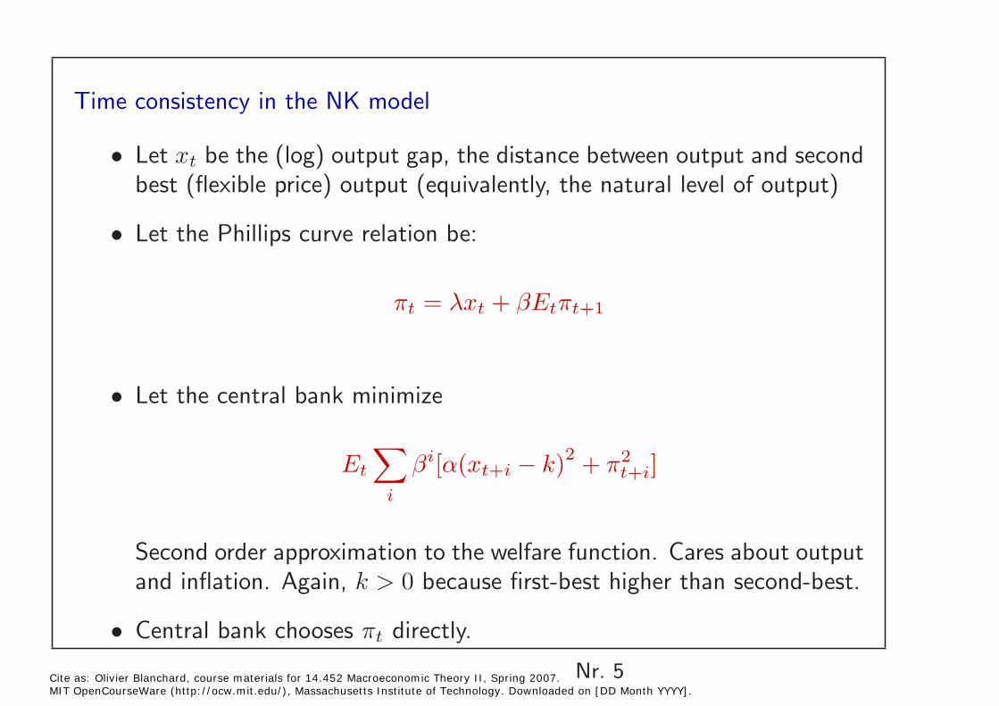
Time consistency in the NK model

Let xt be the (log) output gap, the distance between output and second • best (flexible price) output (equivalently, the natural level of output)

Let the Phillips curve relation be: •

πt = λxt + βEtπt+1

Let the central bank minimize •

� βi[α(xt+i − k)2 + π2 ]Et t+i

i

Second order approximation to the welfare function. Cares about outputand inflation. Again, k > 0 because first-best higher than second-best.

• Central bank chooses πt directly.


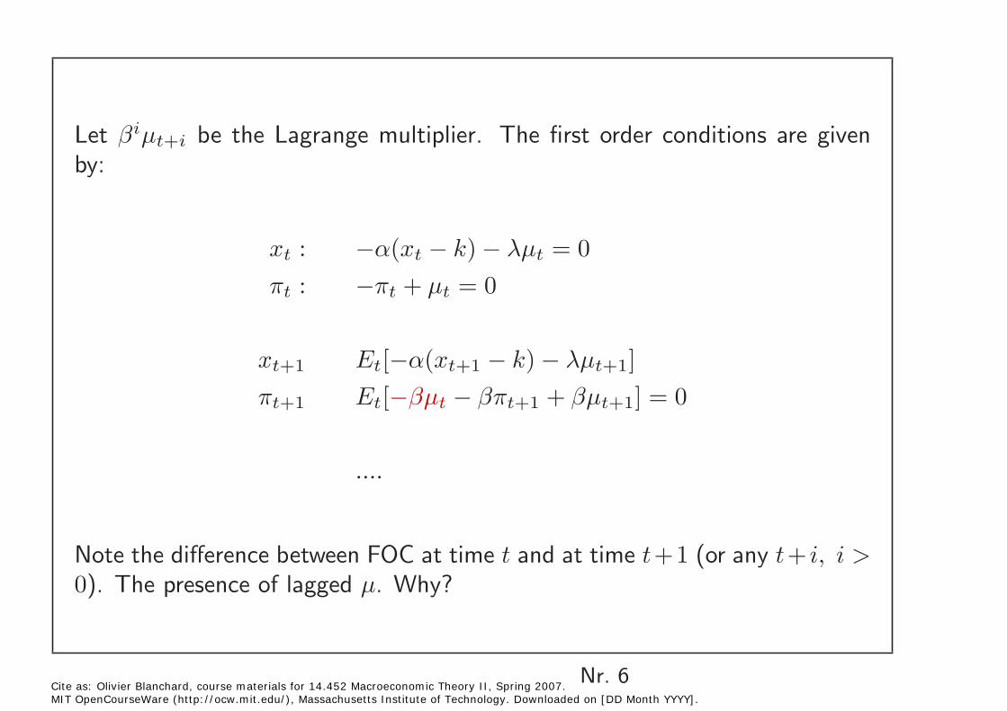
Let βiµt+i be the Lagrange multiplier. The first order conditions are given by:

xt : −α(xt − k) − λµt = 0

πt : −πt + µt = 0

xt+1 Et[−α(xt+1 − k) − λµt+1] πt+1 Et[−βµt − βπt+1 + βµt+1] = 0

....

Note the difference between FOC at time t and at time t +1 (or any t + i, i > 0). The presence of lagged µ. Why?


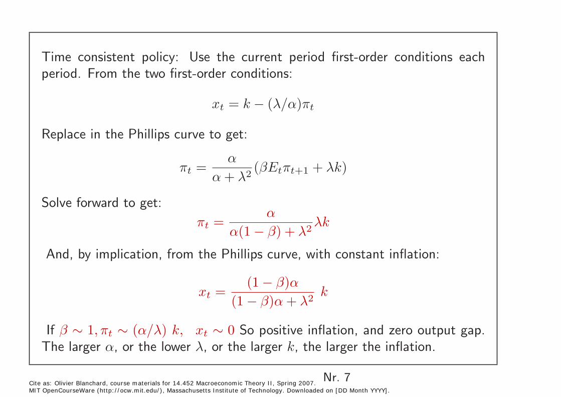
Time consistent policy: Use the current period first-order conditions each period. From the two first-order conditions:

xt = k − (λ/α)πt

Replace in the Phillips curve to get:

α πt = (βEtπt+1 + λk)

α + λ2

Solve forward to get: α

πt = λk α(1 − β) + λ2

And, by implication, from the Phillips curve, with constant inflation:

(1 − β)α xt = k

(1 − β)α + λ2

If β ∼ 1, πt ∼ (α/λ) k, xt ∼ 0 So positive inflation, and zero output gap. The larger α, or the lower λ, or the larger k, the larger the inflation.


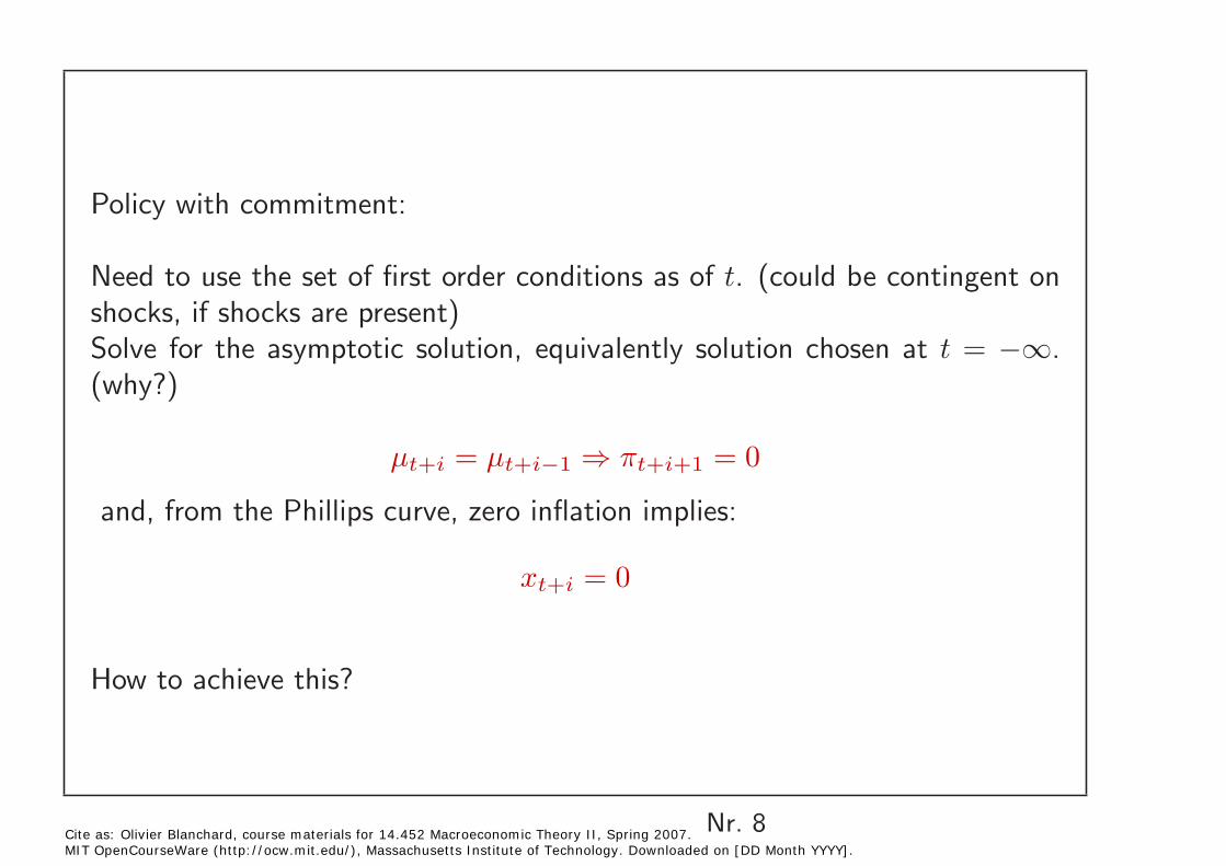
Policy with commitment:

Need to use the set of first order conditions as of t. (could be contingent onshocks, if shocks are present)Solve for the asymptotic solution, equivalently solution chosen at t =−∞. (why?)

µt+i = µt+i−1 πt+i+1 = 0 ⇒

and, from the Phillips curve, zero inflation implies:

xt+i = 0

How to achieve this?


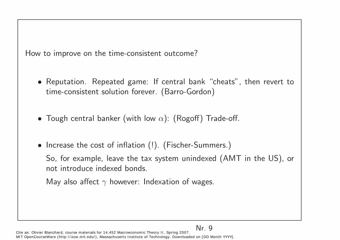
How to improve on the time-consistent outcome?

Reputation. Repeated game: If central bank “cheats”, then revert to • time-consistent solution forever. (Barro-Gordon)

Tough central banker (with low α): (Rogoff) Trade-off.•

Increase the cost of inflation (!). (Fischer-Summers.) •

So, for example, leave the tax system unindexed (AMT in the US), ornot introduce indexed bonds.

May also affect γ however: Indexation of wages.


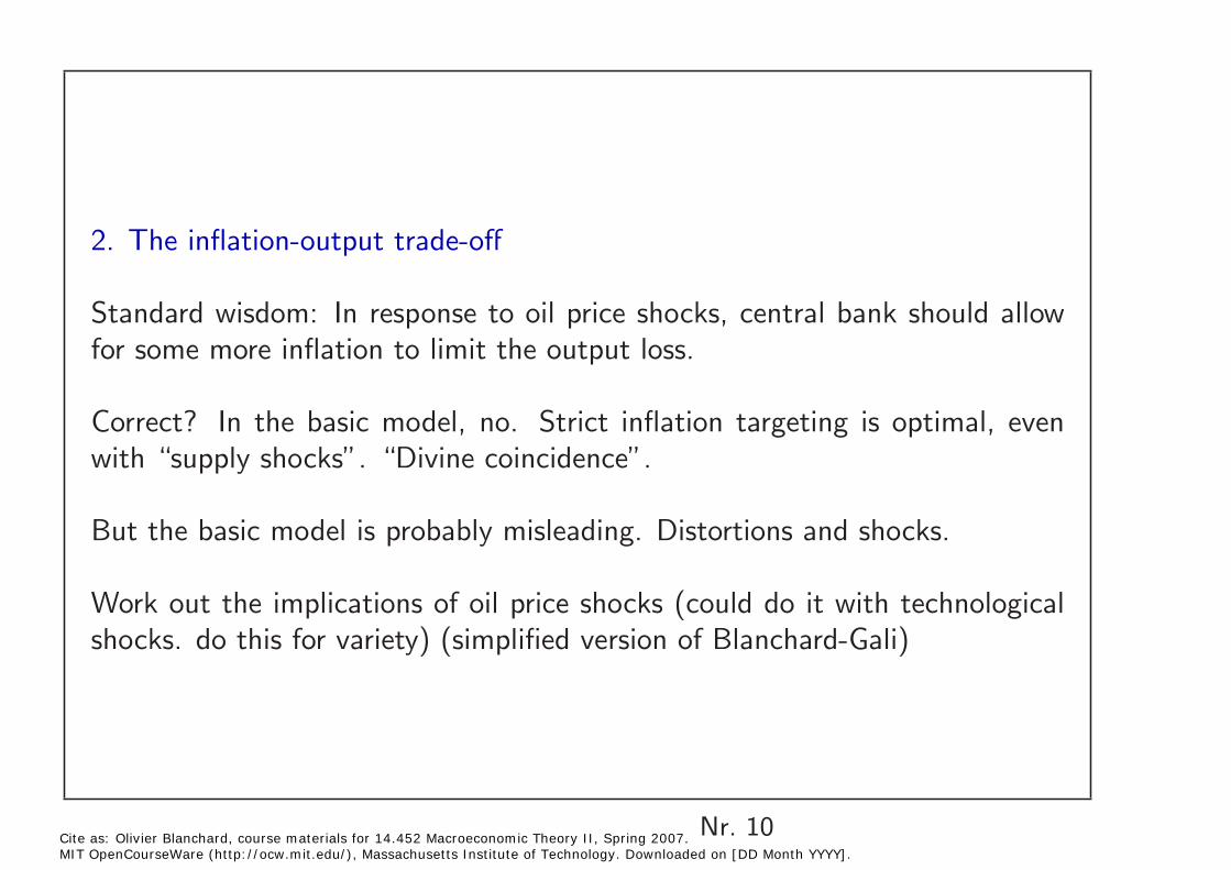
2. The inflation-output trade-off

Standard wisdom: In response to oil price shocks, central bank should allow for some more inflation to limit the output loss.

Correct? In the basic model, no. Strict inflation targeting is optimal, even with “supply shocks”. “Divine coincidence”.

But the basic model is probably misleading. Distortions and shocks.

Work out the implications of oil price shocks (could do it with technological shocks. do this for variety) (simplified version of Blanchard-Gali)


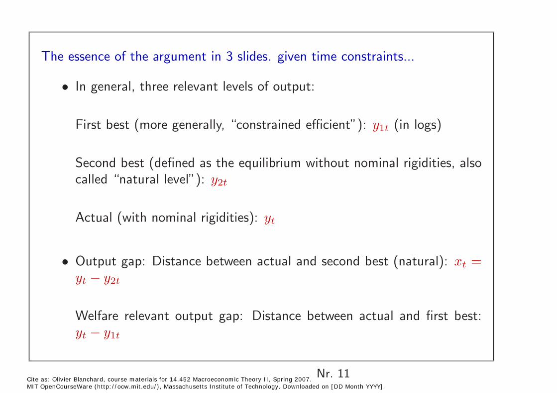
The essence of the argument in 3 slides. given time constraints...

In general, three relevant levels of output: •

First best (more generally, “constrained efficient”): y1t (in logs)

Second best (defined as the equilibrium without nominal rigidities, also called “natural level”): y2t

Actual (with nominal rigidities): yt

Output gap: Distance between actual and second best (natural): xt = • yt − y2t

Welfare relevant output gap: Distance between actual and first best: yt − y1t


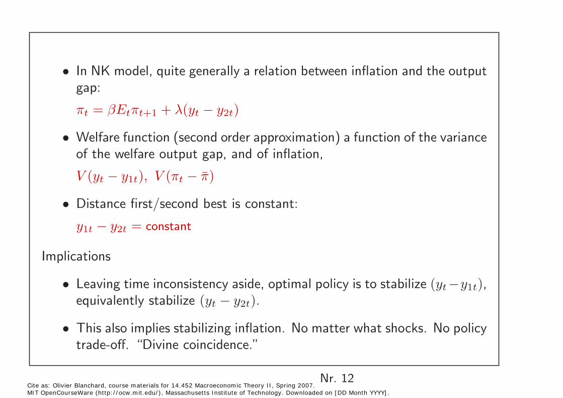
In NK model, quite generally a relation between inflation and the output • gap:

πt = βEtπt+1 + λ(yt − y2t)

Welfare function (second order approximation) a function of the variance • of the welfare output gap, and of inflation,

V (yt − y1t), V (πt − π̄)

Distance first/second best is constant: •

y1t − y2t = constant

Implications

Leaving time inconsistency aside, optimal policy is to stabilize (yt −y1t),• equivalently stabilize (yt − y2t).

This also implies stabilizing inflation. No matter what shocks. No policy• trade-off. “Divine coincidence.”


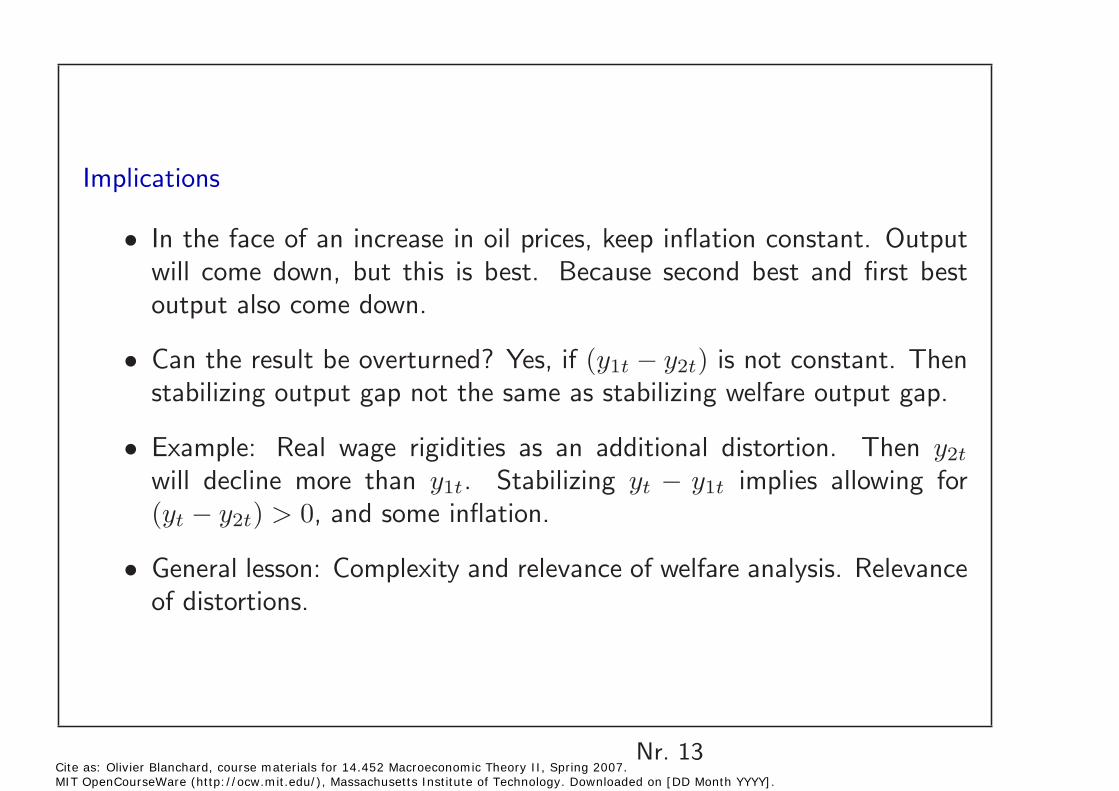
Implications

In the face of an increase in oil prices, keep inflation constant. Output • will come down, but this is best. Because second best and first best output also come down.

Can the result be overturned? Yes, if (y1t − y2t) is not constant. Then • stabilizing output gap not the same as stabilizing welfare output gap.

• Example: Real wage rigidities as an additional distortion. Then y2t

will decline more than y1t. Stabilizing yt − y1t implies allowing for (yt − y2t) > 0, and some inflation.

General lesson: Complexity and relevance of welfare analysis. Relevance • of distortions.


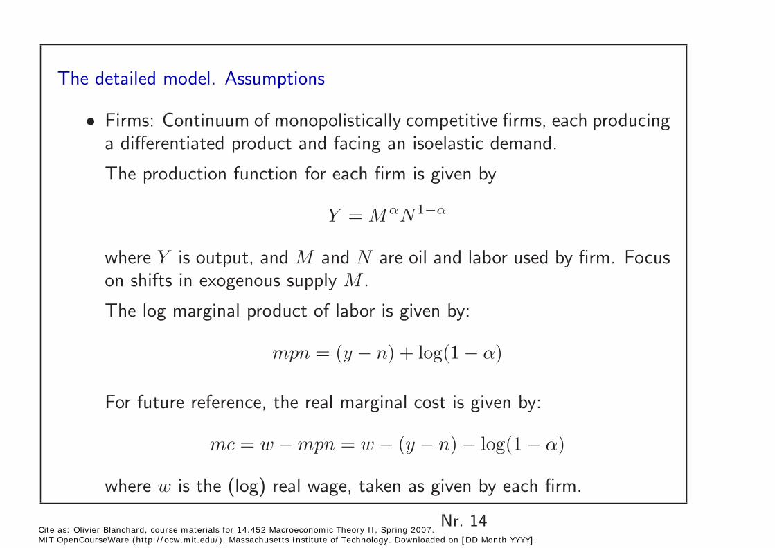
The detailed model. Assumptions

Firms: Continuum of monopolistically competitive firms, each producing • a differentiated product and facing an isoelastic demand.

The production function for each firm is given by

Y = MαN1−α

where Y is output, and M and N are oil and labor used by firm. Focuson shifts in exogenous supply M .

The log marginal product of labor is given by:

mpn = (y − n) + log(1 − α)

For future reference, the real marginal cost is given by:

mc = w − mpn = w − (y − n) − log(1 − α)

where w is the (log) real wage, taken as given by each firm.


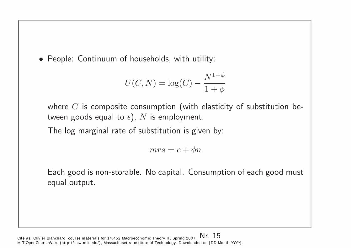
People: Continuum of households, with utility: •

N1+φ

U(C, N) = log(C) − 1 + φ

where C is composite consumption (with elasticity of substitution between goods equal to �), N is employment.

The log marginal rate of substitution is given by:

mrs = c + φn

Each good is non-storable. No capital. Consumption of each good must equal output.

Cite as: Olivier Blanchard, course materials for 14.452 Macroeconomic Theory II, Spring 2007. Nr. 15 MIT OpenCourseWare (http://ocw.mit.edu/), Massachusetts Institute of Technology. Downloaded on [DD Month YYYY].

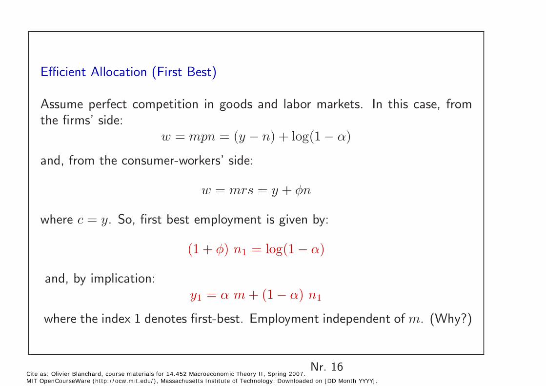
Efficient Allocation (First Best)

Assume perfect competition in goods and labor markets. In this case, from the firms’ side:

w = mpn = (y − n) + log(1 − α)

and, from the consumer-workers’ side:

w = mrs = y + φn

where c = y. So, first best employment is given by:

(1 + φ) n1 = log(1 − α)

and, by implication: y1 = α m + (1 − α) n1

where the index 1 denotes first-best. Employment independent of m. (Why?)


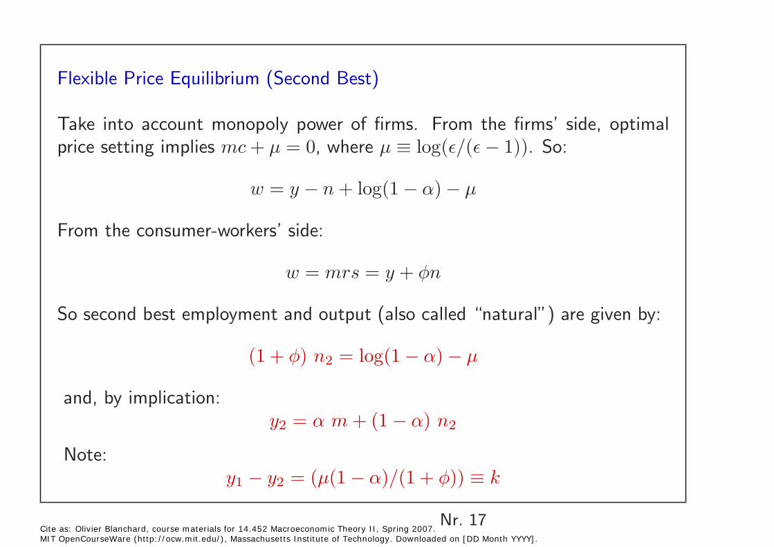
Flexible Price Equilibrium (Second Best)

Take into account monopoly power of firms. From the firms’ side, optimal price setting implies mc + µ = 0, where µ ≡ log(�/(� − 1)). So:

w = y − n + log(1 − α) − µ

From the consumer-workers’ side:

w = mrs = y + φn

So second best employment and output (also called “natural”) are given by:

(1 + φ) n2 = log(1 − α) − µ

and, by implication: y2 = α m + (1 − α) n2

Note: y1 − y2 = (µ(1 − α)/(1 + φ)) ≡ k


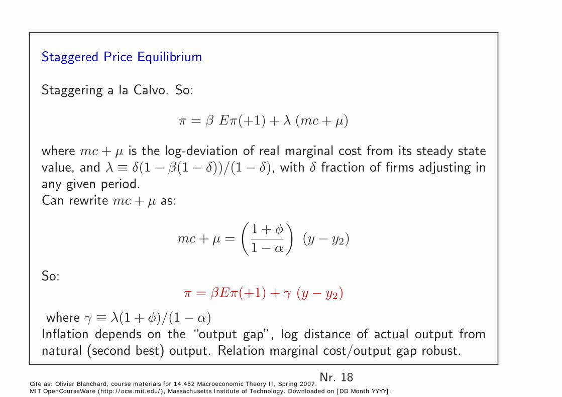
Staggered Price Equilibrium

Staggering a la Calvo. So:

π = β Eπ(+1) + λ (mc + µ)

where mc + µ is the log-deviation of real marginal cost from its steady statevalue, and λ ≡ δ(1 − β(1 − δ))/(1 − δ), with δ fraction of firms adjusting inany given period.Can rewrite mc + µ as:

� 1 + φ

�

mc + µ = 1 − α

(y − y2)

So: π = βEπ(+1) + γ (y − y2)

where γ ≡ λ(1 + φ)/(1 − α) Inflation depends on the “output gap”, log distance of actual output from natural (second best) output. Relation marginal cost/output gap robust.


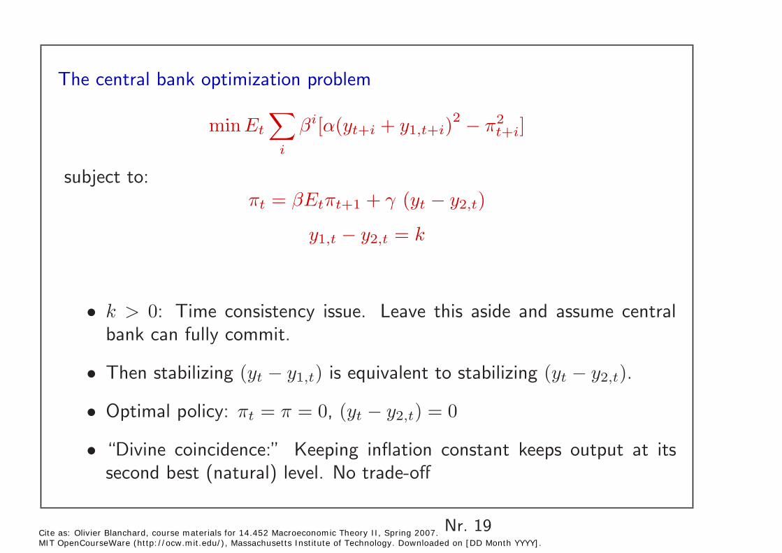
The central bank optimization problem

min Et

� βi[α(yt+i + y1,t+i)

2 − π2 ]t+i

i

subject to: πt = βEtπt+1 + γ (yt − y2,t)

y1,t − y2,t = k

k > 0: Time consistency issue. Leave this aside and assume central • bank can fully commit.

Then stabilizing (yt − y1,t) is equivalent to stabilizing (yt − y2,t).•

Optimal policy: πt = π = 0, (yt − y2,t) = 0 •

• “Divine coincidence:” Keeping inflation constant keeps output at its second best (natural) level. No trade-off


Implications

Even under “supply shocks”, such as an increase in the price of oil (a • decrease in the endowment of oil here). Why?

Output goes down, but so should it. First best also goes down.•

Fairly dramatic result: The central bank can focus just on inflation. It • will have the right implications for activity.

Seems too strong. Even central banks do not follow this principle, and• allow for some more inflation for some time.

Plausible ways out? Something missing from the model?•


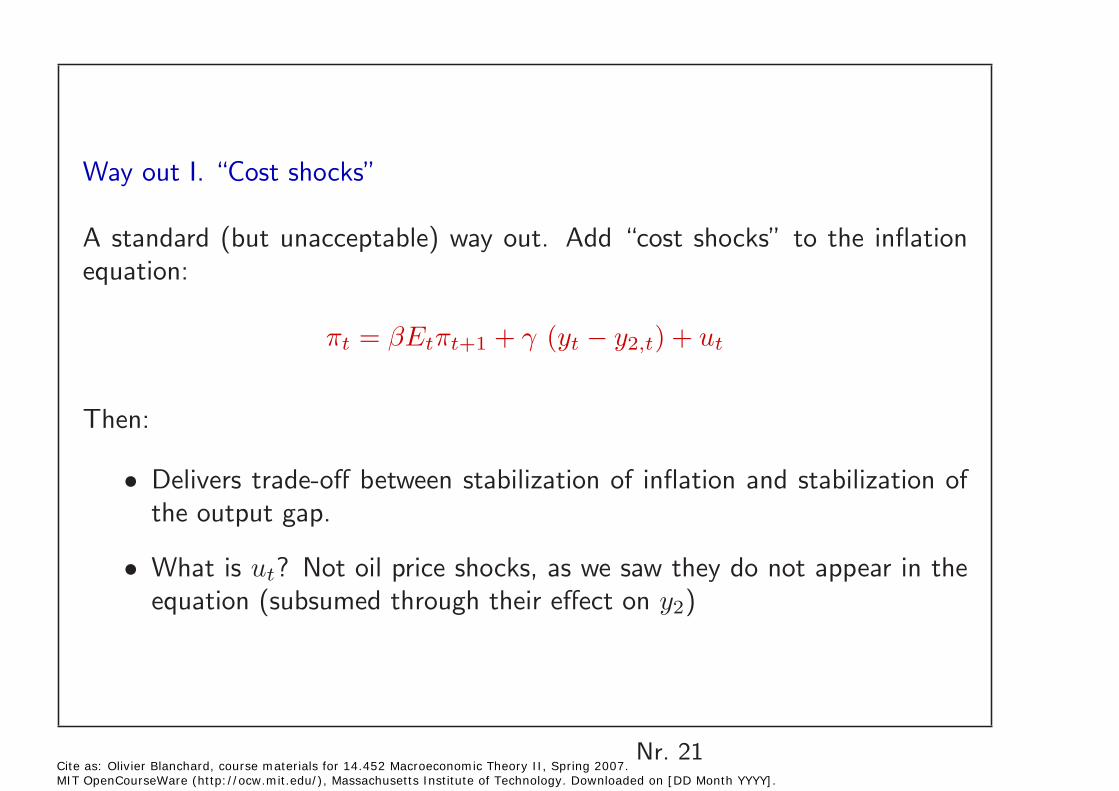
Way out I. “Cost shocks”

A standard (but unacceptable) way out. Add “cost shocks” to the inflation equation:

πt = βEtπt+1 + γ (yt − y2,t) + ut

Then:

Delivers trade-off between stabilization of inflation and stabilization of • the output gap.

What is ut? Not oil price shocks, as we saw they do not appear in the• equation (subsumed through their effect on y2)


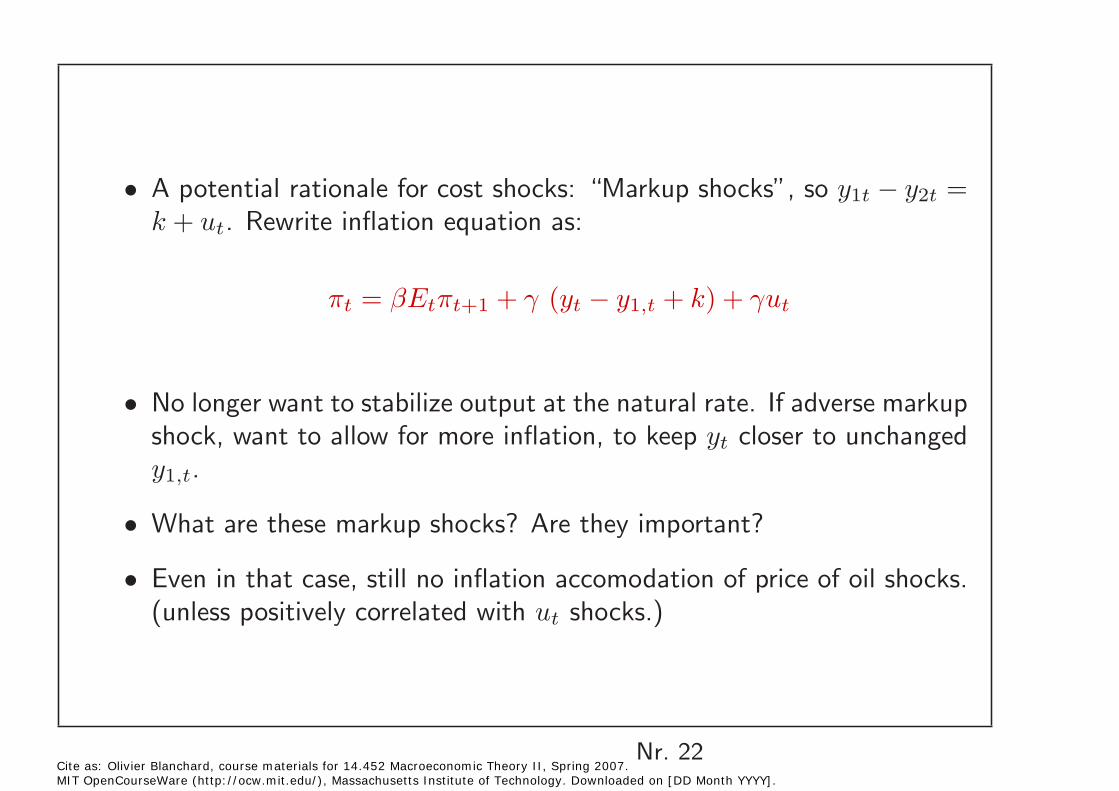
A potential rationale for cost shocks: “Markup shocks”, so y1t − y2t = • k + ut. Rewrite inflation equation as:

πt = βEtπt+1 + γ (yt − y1,t + k) + γut

No longer want to stabilize output at the natural rate. If adverse markup • shock, want to allow for more inflation, to keep yt closer to unchanged y1,t.

What are these markup shocks? Are they important? •

Even in that case, still no inflation accomodation of price of oil shocks. • (unless positively correlated with ut shocks.)


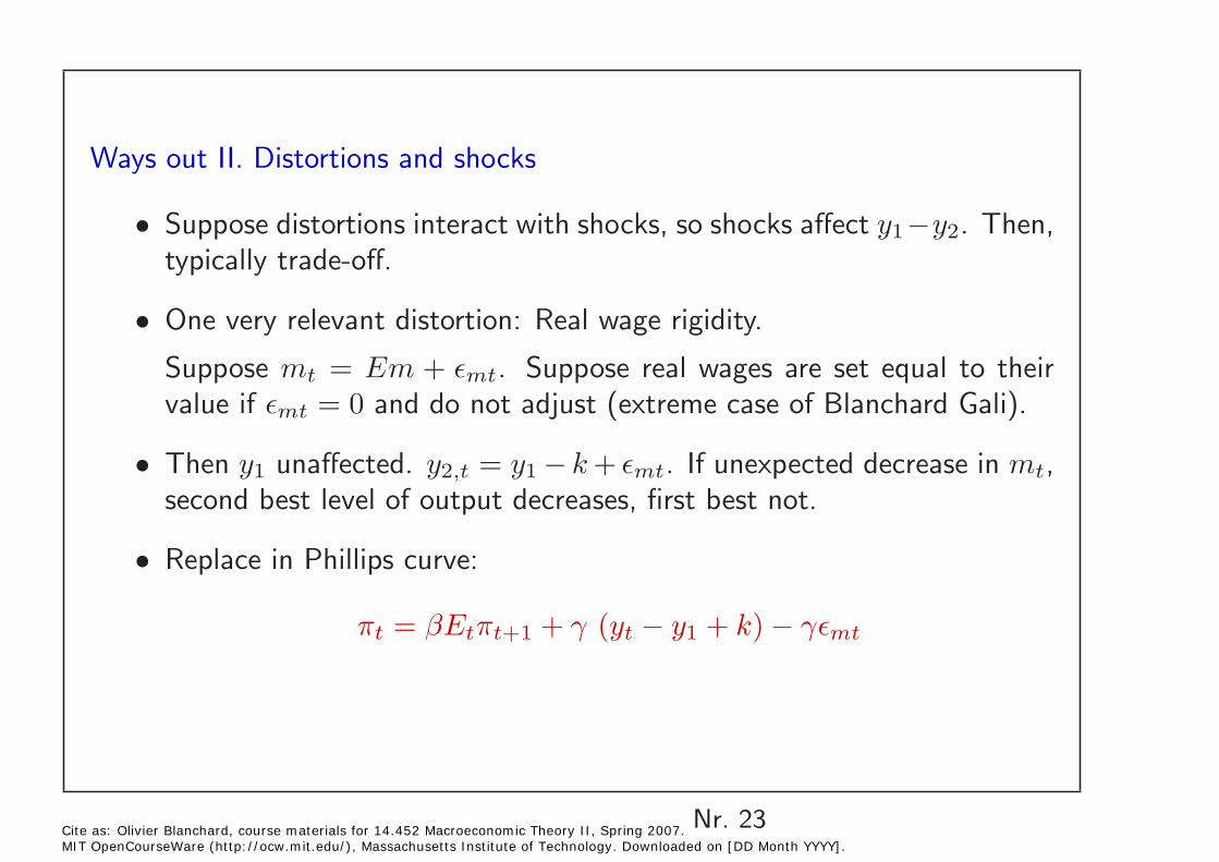
Ways out II. Distortions and shocks

Suppose distortions interact with shocks, so shocks affect y1 −y2. Then,• typically trade-off.

One very relevant distortion: Real wage rigidity.•

Suppose mt = Em + �mt. Suppose real wages are set equal to their value if �mt = 0 and do not adjust (extreme case of Blanchard Gali).

• Then y1 unaffected. y2,t = y1 − k + �mt. If unexpected decrease in mt, second best level of output decreases, first best not.

Replace in Phillips curve: •

πt = βEtπt+1 + γ (yt − y1 + k) − γ�mt


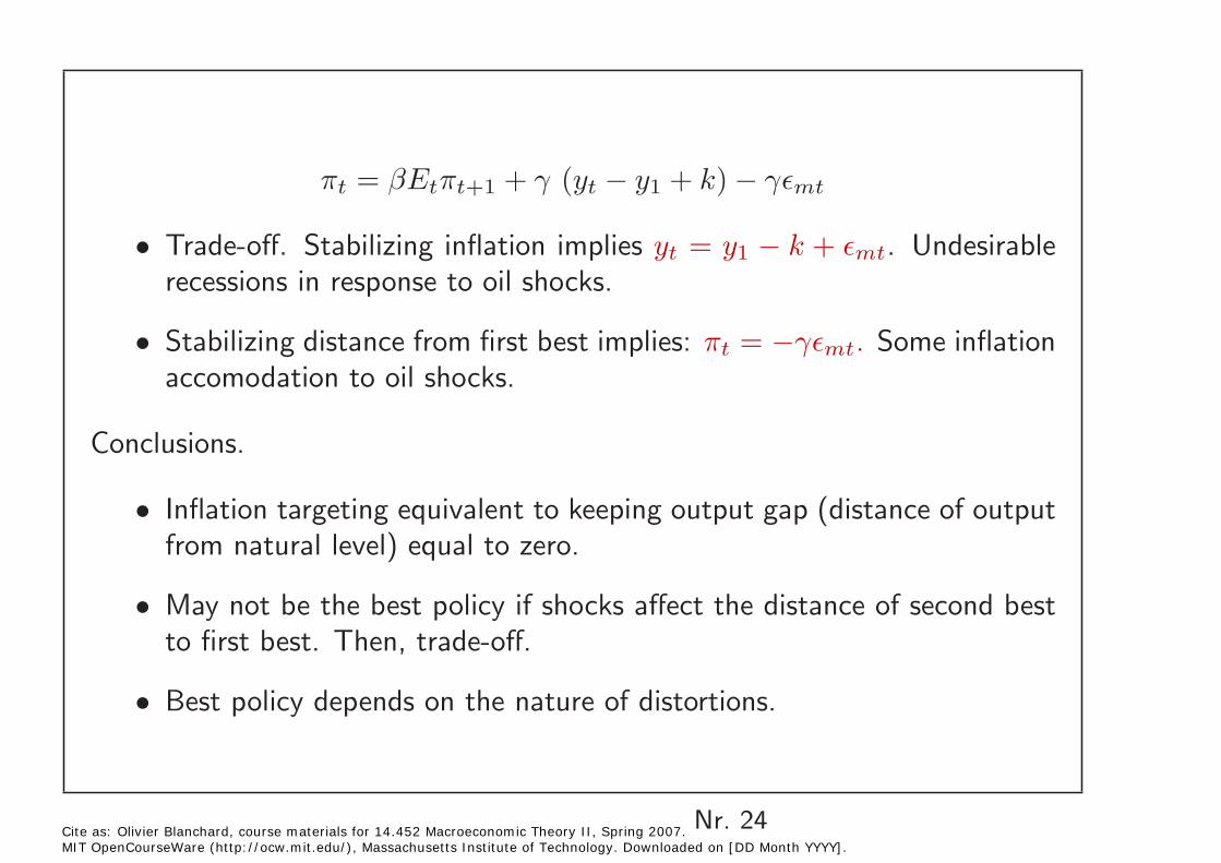
πt = βEtπt+1 + γ (yt − y1 + k) − γ�mt

• Trade-off. Stabilizing inflation implies yt = y1 − k + �mt. Undesirable recessions in response to oil shocks.

• Stabilizing distance from first best implies: πt = −γ�mt. Some inflation accomodation to oil shocks.

Conclusions.

Inflation targeting equivalent to keeping output gap (distance of output • from natural level) equal to zero.

May not be the best policy if shocks affect the distance of second best• to first best. Then, trade-off.

Best policy depends on the nature of distortions.•


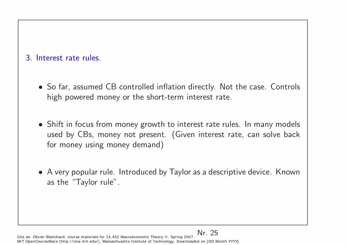
3. Interest rate rules.

So far, assumed CB controlled inflation directly. Not the case. Controls • high powered money or the short-term interest rate.

Shift in focus from money growth to interest rate rules. In many models• used by CBs, money not present. (Given interest rate, can solve back for money using money demand)

A very popular rule. Introduced by Taylor as a descriptive device. Known • as the “Taylor rule”.


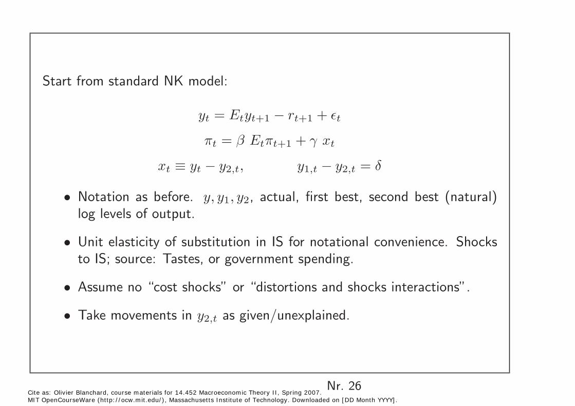
Start from standard NK model:

yt = Etyt+1 − rt+1 + �t

πt = β Etπt+1 + γ xt

xt ≡ yt − y2,t, y1,t − y2,t = δ

• Notation as before. y, y1, y2, actual, first best, second best (natural) log levels of output.

Unit elasticity of substitution in IS for notational convenience. Shocks • to IS; source: Tastes, or government spending.

Assume no “cost shocks” or “distortions and shocks interactions”.•

Take movements in y2,t as given/unexplained. •


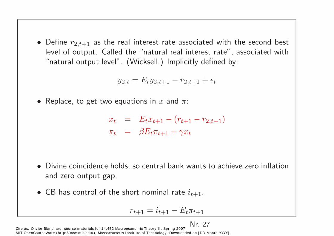
Define r2,t+1 as the real interest rate associated with the second best • level of output. Called the “natural real interest rate”, associated with “natural output level”. (Wicksell.) Implicitly defined by:

y2,t = Ety2,t+1 − r2,t+1 + �t

Replace, to get two equations in x and π:•

xt = Etxt+1 − (rt+1 − r2,t+1) πt = βEtπt+1 + γxt

Divine coincidence holds, so central bank wants to achieve zero inflation • and zero output gap.

CB has control of the short nominal rate it+1.•

rt+1 = it+1 − Etπt+1


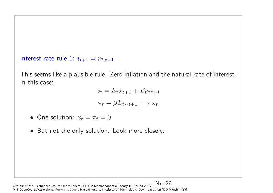
Interest rate rule 1: it+1 = r2,t+1

This seems like a plausible rule. Zero inflation and the natural rate of interest. In this case:

xt = Etxt+1 + Etπt+1

πt = βEtπt+1 + γ xt

One solution: xt = πt = 0 •

But not the only solution. Look more closely: •


Write down the system in matrix form:

1 1 0xt Etxt+1

= + γ γ + β kxtπt Etπt+1

Roots of the matrix A:

λ1λ2 = β, λ1 + λ2 = 1 + γ + β

For uniqueness, the matrix should have both roots inside the circle. If γ ≥ 0, one root is outside. An infinity of converging solutions.

Interpretation: Lack of a nominal anchor.


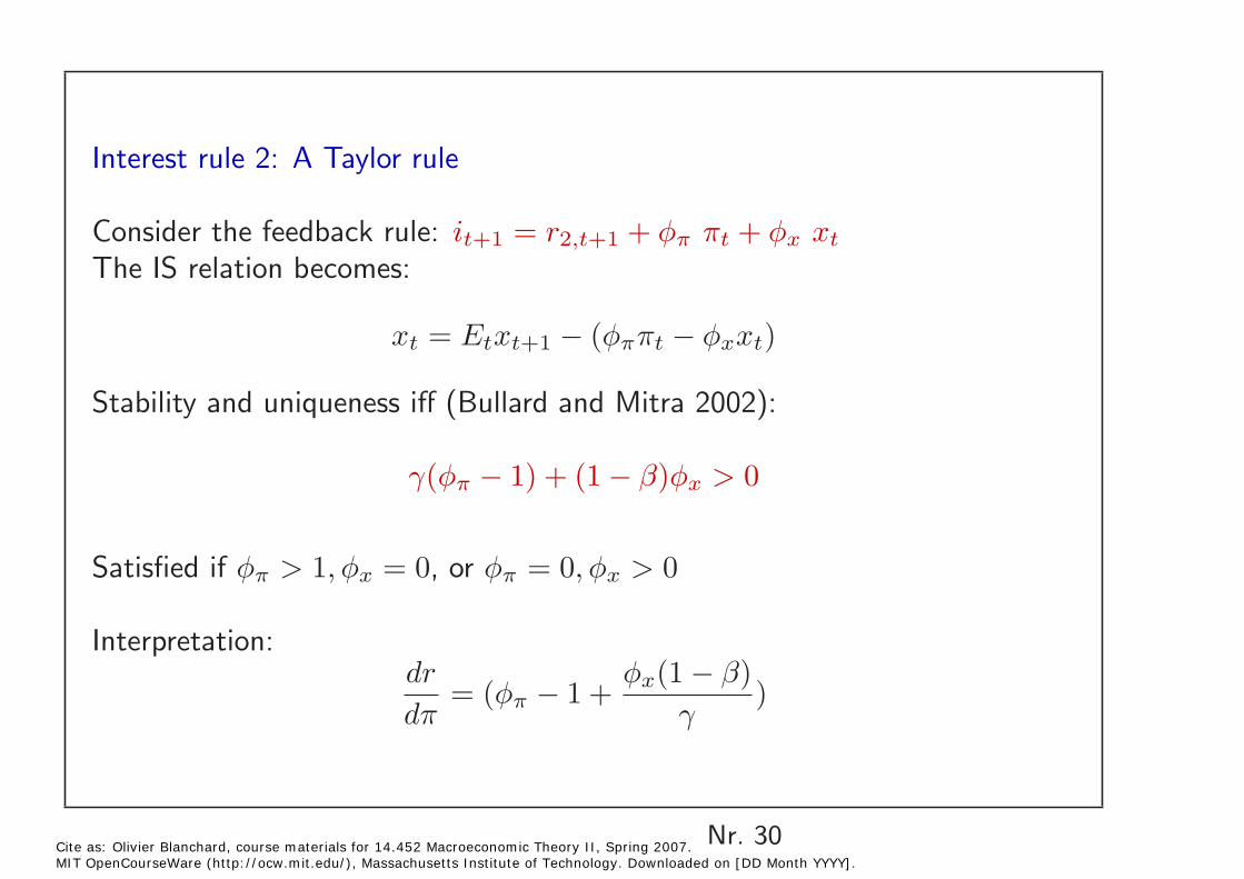
Interest rule 2: A Taylor rule

Consider the feedback rule: it+1 = r2,t+1 + φπ πt + φx xt

The IS relation becomes:

xt = Etxt+1 − (φππt − φxxt)

Stability and uniqueness iff (Bullard and Mitra 2002):

γ(φπ − 1) + (1 − β)φx > 0

Satisfied if φπ > 1, φx = 0, or φπ = 0, φx > 0

Interpretation: dr

= (φπ − 1 + φx(1 − β)

)dπ γ


Implications and extensions

• Optimal rule? Within the model, choose φπ = ∞. Why not?

Observability of r2,t+1. If not, then how good is a Taylor rule, with r̄2• replacing r2,t+1 ?

Robustness to different shocks, lag structures? Gali simulations. 2002.•


olivier blanchard may 12, 2007 - mit opencourseware · olivier blanchard may 12, 2007 nr. 1 cite...

Documents