ols-stata9

8/2/2019 OLS-Stata9

http://slidepdf.com/reader/full/ols-stata9 1/11

Using Stata 9 and Higher for OLS Regression –

Using Stata 9 & Higher for OLS Regression

Introduction . Stata is a popular alternative to SPSS, especially for more advanced statisticaltechniques. This handout shows you how Stata can be used for OLS regression. It assumesknowledge of the statistical concepts that are presented. Several other Stata commands (e.g.

logit , ologit ) often have the same general format and many of the same options.

Rather than specify all options at once, like you do in SPSS, in Stata you often give a series of commands. In some ways, this is more tedious, but it also gives you flexibility in that you don’thave to rerun the entire analysis if you think of something else you want. As the Stata 9 User’sGuide says (p. 43 ) “The user -interface model is type a little, get a little, etc. so that the user isalways in control.”

For the most part, I find that either Stata or SPSS can give me the results I want, but there are sometasks that can be done more easily in one program than the other. For example, I personally preferto do most of my database manipulation in SPSS and then convert the file to Stata, but that is partly

because I am much more familiar with the SPSS commands than their Stata counterparts.Conversely, Stata’s statistical commands are generally far more logical and consistent (andsometimes more powerful) than their SPSS counterparts. Luckily, with the separate Stat Transferprogram, it is very easy to convert SPSS files to Stata and vice-versa.

Get the data. First, open the previously saved data set. (Stata, of course, also has means forentering, editing and otherwise managing data.) You can give the directory and file name, or evenaccess a file that is on the web. For example,

. use http://www.nd.edu/~rwilliam/stats1/statafiles/reg01.dta, clear

Descriptive statistics. There are various ways to get descriptive statistics in Stata. Since you areusing different commands, you want to be careful that you are analyzing the same data throughout,e.g. missing data could change the cases that get analyzed. The correlate command below useslistwise deletion of missing data, which is the same as what the regress command does, i.e. acase is deleted if it is missing data on any of the variables in the analysis.

. correlate income educ jobexp race, means

(obs=20)

Variable | Mean Std. Dev. Min Max-------------+----------------------------------------------------

income | 24.415 9.788354 5 48.3

educ | 12.05 4.477723 2 21jobexp | 12.65 5.460625 1 21race | .5 .5129892 0 1

| income educ jobexp race-------------+------------------------------------

income | 1.0000educ | 0.8457 1.0000

jobexp | 0.2677 -0.1069 1.0000race | -0.5676 -0.7447 0.2161 1.0000

8/2/2019 OLS-Stata9



Regression . Use the regress command for OLS regression (you can abbreviate it as reg ).Specify the DV first followed by the IVs. By default, Stata will report the unstandardized (metric)coefficients.

. regress income educ jobexp race

Source | SS df MS Number of obs = 20-------------+------------------------------ F( 3, 16) = 29.16

Model | 1538.92019 3 512.973396 Prob > F = 0.0000Residual | 281.505287 16 17.5940804 R-squared = 0.8454

-------------+------------------------------ Adj R-squared = 0.8164Total | 1820.42548 19 95.8118671 Root MSE = 4.1945

------------------------------------------------------------------------------income | Coef. Std. Err. t P>|t| [95% Conf. Interval]

-------------+----------------------------------------------------------------educ | 1.981124 .3231024 6.13 0.000 1.296178 2.66607

jobexp | .6419622 .1811106 3.54 0.003 .2580248 1.0259race | .5707931 2.871949 0.20 0.845 -5.517466 6.659052

_cons | -7.863763 5.369166 -1.46 0.162 -19.24589 3.518362------------------------------------------------------------------------------

Confidence Interval. If you want to change the confidence interval, use the level parameter:

. regress income educ jobexp race, level(99)



-------------+------------------------------ Adj R-squared = 0.8164

Total | 1820.42548 19 95.8118671 Root MSE = 4.1945


-------------+----------------------------------------------------------------educ | 1.981124 .3231024 6.13 0.000 1.037413 2.924835

jobexp | .6419622 .1811106 3.54 0.003 .1129776 1.170947race | .5707931 2.871949 0.20 0.845 -7.817542 8.959128

_cons | -7.863763 5.369166 -1.46 0.162 -23.54593 7.8184------------------------------------------------------------------------------

As an alternative, you could use the set level command before regress :

. set level 99


8/2/2019 OLS-Stata9



Standardized coefficients. To get the standardized coefficients, add the beta parameter:

. regress income educ jobexp race, beta


Model | 1538.92019 3 512.973396 Prob > F = 0.0000Residual | 281.505287 16 17.5940804 R-squared = 0.8454-------------+------------------------------ Adj R-squared = 0.8164

Total | 1820.42548 19 95.8118671 Root MSE = 4.1945

------------------------------------------------------------------------------income | Coef. Std. Err. t P>|t| Beta

-------------+----------------------------------------------------------------educ | 1.981124 .3231024 6.13 0.000 .9062733

jobexp | .6419622 .1811106 3.54 0.003 .3581312race | .5707931 2.871949 0.20 0.845 .0299142

_cons | -7.863763 5.369166 -1.46 0.162 .------------------------------------------------------------------------------

NOTE: The listcoef command from Long and Freese’s spost9 package of routines (typefindit spost9 from within Stata) provides alternative ways of standardizing coefficients.

Incidentally, you do not have to repeat the entire command when you change a parameter (indeed,if the data set is large, you don’t want to repeat the entire command, because then Stata will redo allthe calculations.) The last three regressions could have been executed via the commands


. regress, level(99)

. regress, beta

Also, if you just type regress Stata will “replay” (print out again) your earlier results. VIF & Tolerances. Use the vif command to get the variance inflation factors (VIFs) and thetolerances (1/VIF). vif is one of many post-estimation commands. You run it AFTER running aregression. It uses information Stata has stored internally.

. vif

Variable | VIF 1/VIF-------------+----------------------

race | 2.34 0.426622educ | 2.26 0.442403

jobexp | 1.06 0.946761

-------------+----------------------Mean VIF | 1.89

NOTE: vif only works after regress, which is unfortunate because the information it offers can beuseful with many other commands, e.g. logit . Phil Ender’s collin command gives moreinformation and can be used with estimation commands besides regress , e.g.

. collin educ jobexp race if !missing(income)

8/2/2019 OLS-Stata9



Hypothesis testing. Stata has some very nice hypothesis testing procedures; indeed I think it hassome big advantages over SPSS here. Again, these are post-estimation commands; you run theregression first and then do the hypothesis tests. To test whether the effects of educ and/or jobexpdiffer from zero (i.e. to test β1 = β 2 = 0), use the test command:

. test educ jobexp

( 1) educ = 0( 2) jobexp = 0

F( 2, 16) = 27.07Prob > F = 0.0000

The test command does what is known as a Wald test. In this case, it gives the same result as anincremental F test.

If you want to test whether the effects of educ and jobexp are equal, i.e. β 1 = β 2,

. test educ=jobexp

( 1) educ - jobexp = 0

F( 1, 16) = 12.21Prob > F = 0.0030

If you want to see what the coefficients of the constrained model are, add the coef parameter:

. test educ=jobexp, coef

( 1) educ - jobexp = 0

F( 1, 16) = 12.21Prob > F = 0.0030

Constrained coefficients

------------------------------------------------------------------------------| Coef. Std. Err. z P>|z| [95% Conf. Interval]

-------------+----------------------------------------------------------------educ | .9852105 .1521516 6.48 0.000 .6869989 1.283422

jobexp | .9852105 .1521516 6.48 0.000 .6869989 1.283422race | -6.692116 1.981712 -3.38 0.001 -10.5762 -2.808031

_cons | 3.426358 4.287976 0.80 0.424 -4.977921 11.83064------------------------------------------------------------------------------

The testparm and cnsreg commands can also be used to achieve the same results. Stata alsohas other commands (e.g. testnl ) that can be used to test even more complicated hypotheses.

8/2/2019 OLS-Stata9



Nested models. Alternatively, the nestreg command will compute incremental F-tests. (If you are stuck with Stata 8, Paul Bern’s hireg command performs a similar function.) Thenestreg command is particularly handy if you are estimating a series/hierarchy of models andwant to see the regression results for each one. To again test whether the effects of educ and/or

jobexp differ fr om zero (i.e. to test β 1 = β 2 = 0), the nestreg command would be

. nestreg: regress income (race) (educ jobexp)

Block 1: race




------------------------------------------------------------------------------

income | Coef. Std. Err. t P>|t| [95% Conf. Interval]-------------+----------------------------------------------------------------race | -10.83 3.702823 -2.92 0.009 -18.60934 -3.050657

_cons | 29.83 2.618291 11.39 0.000 24.32917 35.33083------------------------------------------------------------------------------

Block 2: educ jobexp





-------------+----------------------------------------------------------------race | .5707931 2.871949 0.20 0.845 -5.517466 6.659052educ | 1.981124 .3231024 6.13 0.000 1.296178 2.66607

jobexp | .6419622 .1811106 3.54 0.003 .2580248 1.0259_cons | -7.863763 5.369166 -1.46 0.162 -19.24589 3.518362

------------------------------------------------------------------------------

+-------------------------------------------------------------+| | Block Residual Change |

| Block | F df df Pr > F R2 in R2 ||-------+-----------------------------------------------------|| 1 | 8.55 1 18 0.0090 0.3221 || 2 | 27.07 2 16 0.0000 0.8454 0.5232 |+-------------------------------------------------------------+

nestreg works with several other commands (e.g. logit ) and has additional options (e.g.lrtable , store ) that can be very useful.

8/2/2019 OLS-Stata9



Partial and SemiPartial Correlations. There is a separate Stata routine, pcorr , which gives thepartial correlations but, prior to Stata 11, did not give the semipartials. I wrote a routine, pcorr2 ,which gives both the partial and semipartial correlations. The pcorr command in Stata 11 took some of my code from pcorr2 and now gives very similar output.

. pcorr2 income educ jobexp race

(obs=20)

Partial and Semipartial correlations of income with

Variable | Partial SemiP Partial^2 SemiP^2 Sig.-------------+------------------------------------------------------------

educ | 0.8375 0.6028 0.7015 0.3634 0.000jobexp | 0.6632 0.3485 0.4399 0.1214 0.003

race | 0.0496 0.0195 0.0025 0.0004 0.845

Stepwise Regression. The sw prefix lets you do stepwise regression and can be used with manycommands besides regress . Here is how to do backwards stepwise regression. Use the pr (probability for removal) parameter to specify how significant the coefficient must be to avoidremoval. Note that SPSS is better if you need more detailed step by step results.

. sw, pr(.05): regress income educ jobexp race

begin with full modelp = 0.8450 >= 0.0500 removing race

Source | SS df MS Number of obs = 20

-------------+------------------------------ F( 2, 17) = 46.33Model | 1538.22521 2 769.112605 Prob > F = 0.0000Residual | 282.200265 17 16.6000156 R-squared = 0.8450



-------------+----------------------------------------------------------------educ | 1.933393 .2099494 9.21 0.000 1.324911 2.541875

jobexp | .6493654 .1721589 3.77 0.002 .150409 1.148322_cons | -7.096855 3.626412 -1.96 0.067 -17.60703 3.413322

------------------------------------------------------------------------------

8/2/2019 OLS-Stata9



To do forward stepwise instead, use the pe (probability for entry) parameter to specify the level of significance for entering the model.

. sw, pe(.05): regress income educ jobexp racebegin with empty model

p = 0.0000 < 0.0500 adding educp = 0.0015 < 0.0500 adding jobexp





-------------+----------------------------------------------------------------educ | 1.933393 .2099494 9.21 0.000 1.324911 2.541875

jobexp | .6493654 .1721589 3.77 0.002 .150409 1.148322_cons | -7.096855 3.626412 -1.96 0.067 -17.60703 3.413322------------------------------------------------------------------------------

Sample Selection. In SPSS, you can use Select If or Filter commands to control whichcases get analyzed. Stata also has a variety of means for handling sample selection. One of themost common ways is the use of the if parameter on commands. So if, for example, we onlywanted to analyze whites, we could type

. reg income educ jobexp if race==0

Source | SS df MS Number of obs = 10-------------+------------------------------ F( 2, 7) = 18.39Model | 526.810224 2 263.405112 Prob > F = 0.0016

Residual | 100.250763 7 14.3215375 R-squared = 0.8401-------------+------------------------------ Adj R-squared = 0.7944

Total | 627.060987 9 69.673443 Root MSE = 3.7844


-------------+----------------------------------------------------------------educ | 2.459518 .5265393 4.67 0.002 1.21445 3.704585

jobexp | .5314947 .2216794 2.40 0.048 .0073062 1.055683_cons | -13.91281 7.827619 -1.78 0.119 -32.42219 4.596569

------------------------------------------------------------------------------

8/2/2019 OLS-Stata9



Separate Models for Groups. Or, suppose we wanted to estimate separate models for blacks andwhites. In SPSS, we could use the Split File command. In Stata, we can use the by command (data must be sorted first if they aren’t sorted already ):

. sort race

. by race: reg income educ jobexp

_______________________________________________________________________________-> race = white




------------------------------------------------------------------------------

income | Coef. Std. Err. t P>|t| [95% Conf. Interval]-------------+----------------------------------------------------------------educ | 2.459518 .5265393 4.67 0.002 1.21445 3.704585

jobexp | .5314947 .2216794 2.40 0.048 .0073062 1.055683_cons | -13.91281 7.827619 -1.78 0.119 -32.42219 4.596569

------------------------------------------------------------------------------

_______________________________________________________________________________-> race = black





-------------+----------------------------------------------------------------educ | 1.788485 .4541661 3.94 0.006 .7145528 2.862417

jobexp | .7074115 .3237189 2.19 0.065 -.058062 1.472885_cons | -6.500947 6.406053 -1.01 0.344 -21.64886 8.646961

------------------------------------------------------------------------------

As an alternative, rather than using separate sort and by commands, you could use bysort :

. bysort race: reg income educ jobexp

Analyzing Means, Correlations and Standard Deviations in Stata. Sometimes you mightwant to replicate or modify a published analysis. You don’t have the original data, but the author shave published their means, correlations and standard deviations. SPSS lets you input and analyzethese directly. In Stata, you must first create a pseudo-replication (my term, explained in amoment) of the original data. You use Stata’s corr2data command for this.

8/2/2019 OLS-Stata9



For example, in their classic 1985 pape r, “ Ability grouping and contextual determinants of educational expec tations in Israel,” Shavit and Williams examined the effect of ethnicity and othervariables on the achievement of Israeli school children. There are two main ethnic groups in Israel:the Ashkenazim - of European birth or extraction - and the Sephardim, most of whose families

immigrated to Israel during the early fifties from North Africa, Iraq, and other Mid-easterncountries. Their variables included:X1 - Ethnicity (SPHRD) - a dummy variable coded 1 if the respondent or both his parents

were born in an Asian or North African country, 0 otherwiseX2 - Parental Education (PARED) - A scale which ranges from a low of 0 to a high of 1.697X3 - Scholastic Aptitude (APTD) - A composite score based on seven achievement tests.Y - Grades (GRADES) - Respondent's grade-point average during the first trimester of

eighth grade. This scale ranges from a low of 4 to a high of 10.

Shavit and Williams’ published analysis included the following information for students who wereability grouped in their classes.

De scr iptive Statistics

.44000 .50000 10609

.82000 .46000 106096.46000 2.11000 106097.12000 1.42000 10609

SephardimParental Education ScaleScholastic AptitudeGrade Point Average

MeanStd.

Deviation N

Correlations

1.000 -.590 -.460 -.260-.590 1.000 .530 .330-.460 .530 1.000 .720-.260 .330 .720 1.000

SephardimParental Education ScaleScholastic AptitudeGrade Point Average

Pearson CorrelationSephardim

ParentalEducation

ScaleScholasticAptitude

GradePoint

Average

To create a pseudo-replication of this data in Stata, we do the following. (I find that entering thedata is most easily done via the input matrix by hand submenu of Data ).

. * First, input the means, sds, and correlations

. matrix input Mean = (.44,.82,6.46,7.12)

. matrix input SD = (.5,.46,2.11,1.42)

. matrix input Corr = (1.00,-.59,-.46,-.26\-.59,1.00,.53,.33\-

.46,.53,1.00,.72\-.26,.33,.72,1.00)

. * Now use corr2data to create a pseudo-simulation of the data

. corr2data sphrd pared aptd grades, n(10609) means(Mean) corr(Corr) sds(SD)(obs 10609)

8/2/2019 OLS-Stata9



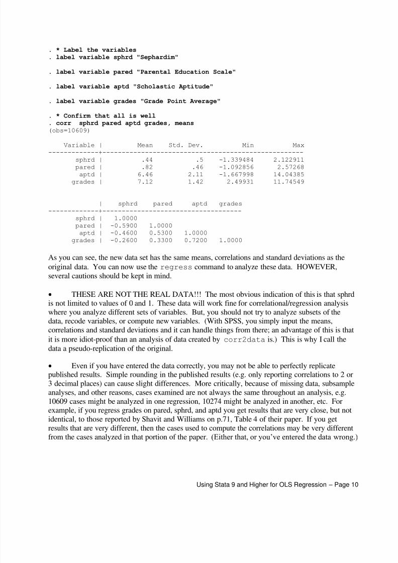
. * Label the variables

. label variable sphrd "Sephardim"

. label variable pared "Parental Education Scale"

. label variable aptd "Scholastic Aptitude"

. label variable grades "Grade Point Average"

. * Confirm that all is well

. corr sphrd pared aptd grades, means(obs=10609)

Variable | Mean Std. Dev. Min Max-------------+----------------------------------------------------

sphrd | .44 .5 -1.339484 2.122911pared | .82 .46 -1.092856 2.57268

aptd | 6.46 2.11 -1.667998 14.04385grades | 7.12 1.42 2.49931 11.74549

| sphrd pared aptd grades-------------+------------------------------------

sphrd | 1.0000pared | -0.5900 1.0000

aptd | -0.4600 0.5300 1.0000grades | -0.2600 0.3300 0.7200 1.0000

As you can see, the new data set has the same means, correlations and standard deviations as theoriginal data. You can now use the regress command to analyze these data. HOWEVER,several cautions should be kept in mind.

THESE ARE NOT THE REAL DATA!!! The most obvious indication of this is that sphrdis not limited to values of 0 and 1. These data will work fine for correlational/regression analysiswhere you analyze different sets of variables. But, you should not try to analyze subsets of thedata, recode variables, or compute new variables. (With SPSS, you simply input the means,correlations and standard deviations and it can handle things from there; an advantage of this is thatit is more idiot-proof than an analysis of data created by corr2data is.) This is why I call thedata a pseudo-replication of the original.

Even if you have entered the data correctly, you may not be able to perfectly replicatepublished results. Simple rounding in the published results (e.g. only reporting correlations to 2 or3 decimal places) can cause slight differences. More critically, because of missing data, subsample

analyses, and other reasons, cases examined are not always the same throughout an analysis, e.g.10609 cases might be analyzed in one regression, 10274 might be analyzed in another, etc. Forexample, if you regress grades on pared, sphrd, and aptd you get results that are very close, but notidentical, to those reported by Shavit and Williams on p.71, Table 4 of their paper. If you getresults that are very different, then the cases used to compute the correlations may be very differentfrom the cases analyzed in that portion of the paper. (Either that, or you’ve entered the data wrong.)

8/2/2019 OLS-Stata9



Adding to Stata. SPSS is pretty much a closed- ended program. If it doesn’t have what you wantalready built-in, you are out of luck. With Stata, however, it is possible to write your own routineswhich add to the functionality of the program. Further, many such routines are publicly availableand can be easily installed on your machine. I’ve often found that something that SPSS had andStata did not could be added to Stata. For example, Stata does NOT have a built-in command for

computing semipartial correlations. To see if such a routine exists, from within Stata you can typefindit semipartial

The findit command will give you listings of programs that have the keyword semipartialassociated with them. It will also give you FAQs and Stata help associated with the term. Amongthe things that will pop up is my very own pcorr2 , which is an enhanced version of Stata’spcorr command in that it computes both partial and semipartial correlations ( pcorr only doespartial correlations). Usually a routine includes a brief description and you can view its help file.Sometimes routines are part of a package of related routines and you install the entire package.Once you have found a routine that sounds like what you want, you can easily install it. You can

also easily uninstall if you decide you do not want it.

A couple of cautions:

User written routines are not officially supported by Stata. Indeed, it is entirely possiblethat such a routine has bugs or gives incorrect results, at least under certain conditions. Most of theroutines I have installed seem to work fine, but I have found a few problems. You might want todouble-check results against SPSS or published findings. If a command works on one machine but not another, it is probably because that command

is not installed on both machines. For example, if the pcorr2 command was not working, typefindit pcorr2 and then install it on your machine. (A possible complication is that you may

find newer and older versions of the same command, and you may even find two differentcommands with the same name. So, check to make sure you are getting what you think you aregetting. If you ever write your own routine, I suggest you try something like findit myprog tomake sure somebody isn’t already using the name you had in mind.)

Other Comments.

Unlike SPSS, Stata is picky about case, e.g. findit pcorr2 works, Findit pcorr2 does not. Income , income and INCOME would all be different variable names. Stata 8 added a menu-structure that made it more SPSS-like. This can be very handy for

commands you are not familiar with. For commands I know, however, I generally find it easier justto type the command in directly. Although not as essential as they used to be, I find it helpful to install the StataQuest

routines. If not already installed, type findit quest7 and install quest1, quest2 and quest3.Then, from within Stata, the command quest on will activate a Stataquest submenu underthe User menu that has various helpful features. There are various other options for the regress command and several other post-

estimation commands that can be useful. See my notes for graduate statistics II.

ols-stata9

Documents