omi ozone profile retrievals - · acpd 9, 22693–22738, 2009 omi ozone proﬁle retrievals x. liu...

ACPD9, 22693–22738, 2009

OMI ozone profileretrievals

X. Liu et al.

Title Page

Abstract Introduction

Conclusions References

Tables Figures

J I

J I

Back Close

Full Screen / Esc

Printer-friendly Version

Interactive Discussion

Atmos. Chem. Phys. Discuss., 9, 22693–22738, 2009www.atmos-chem-phys-discuss.net/9/22693/2009/© Author(s) 2009. This work is distributed underthe Creative Commons Attribution 3.0 License.

AtmosphericChemistry

and PhysicsDiscussions

This discussion paper is/has been under review for the journal Atmospheric Chemistryand Physics (ACP). Please refer to the corresponding final paper in ACP if available.

Ozone profile retrievals from the OzoneMonitoring Instrument

X. Liu1,2,3, P. K. Bhartia3, K. Chance2, R. J. D. Spurr4, and T. P. Kurosu2

1Goddard Earth Sciences and Technology Center, University of Maryland, Baltimore County,Baltimore, Maryland, USA2Harvard-Smithsonian Center for Astrophysics, Cambridge, Massachusetts, USA3NASA Goddard Space Flight Center, Greenbelt, Maryland, USA4RT Solutions Inc., Cambridge, Massachusetts, USA

Received: 18 August 2009 – Accepted: 3 October 2009 – Published: 27 October 2009

Correspondence to: X. Liu ([email protected])

Published by Copernicus Publications on behalf of the European Geosciences Union.

22693

http://www.atmos-chem-phys-discuss.net

http://www.atmos-chem-phys-discuss.net/9/22693/2009/acpd-9-22693-2009-print.pdf

http://www.atmos-chem-phys-discuss.net/9/22693/2009/acpd-9-22693-2009-discussion.html

http://creativecommons.org/licenses/by/3.0/

ACPD9, 22693–22738, 2009


X. Liu et al.

Title Page



Tables Figures

J I

J I

Back Close

Full Screen / Esc



Abstract

Ozone profiles from the surface to about 60 km are retrieved from Ozone MonitoringInstrument (OMI) ultraviolet radiances using the optimal estimation technique. OMIprovides daily ozone profiles for the entire sunlit portion of the earth at a horizontalresolution of 13 km×48 km for the nadir position. The retrieved profiles have sufficient5

accuracy in the troposphere to see ozone perturbations caused by convection, biomassburning and anthropogenic pollution, and to track their spatiotemporal transport. How-ever, to achieve such accuracy it has been necessary to calibrate OMI radiances care-fully (using two days of Aura/Microwave Limb Sounder data taken in the tropics). Theretrieved profiles contain ∼6–7 degrees of freedom for signal, with 5–7 in the strato-10

sphere and 0–1.5 in the troposphere. Vertical resolution varies from 7–11 km in thestratosphere to 10–14 km in the troposphere. Retrieval precisions range from 1% inthe middle stratosphere to 10% in the lower stratosphere and troposphere. Solutionerrors (i.e., root sum square of precisions and smoothing errors) vary from 1–6% inthe middle stratosphere to 6–35% in the troposphere, and are dominated by smooth-15

ing errors. Total, stratospheric, and tropospheric ozone columns can be retrieved withsolution errors typically in the few Dobson unit range at solar zenith angles less than80◦.

1 Introduction

Total ozone column and ozone profiles have been retrieved since 1970 from about20

a dozen Backscattered Ultraviolet (BUV) instruments that have flown on NASA andNOAA satellites. These instruments measure at 12 discrete 1 nm wide wavelengthbands in the 250–340 nm range, providing vertical information from the ozone densitypeak (20–25 km) to ∼50 km plus the ozone column down to the surface/cloud altitude(Bhartia et al., 1996). Chance et al. (1991, 1997) showed that it may be possible to ex-25

tend the ozone profile information to lower altitudes, including the troposphere, by using

22694





ACPD9, 22693–22738, 2009


X. Liu et al.

Title Page



Tables Figures

J I

J I

Back Close

Full Screen / Esc



high spectral resolution (<0.5 nm) hyperspectral (contiguous in wavelength) data frominstruments like the Global Ozone Monitoring Experiment (GOME). Over the years,several groups, have developed physically based retrieval algorithms to retrieve ozoneprofiles from GOME radiances (Munro et al., 1998; Hoogen et al., 1999; Hasekampand Landgraf, 2001; van der A et al., 2002; Liu et al., 2005). Meijer et al. (2006) evalu-5

ated ozone profiles retrieved from these algorithms and concluded that though ozoneprofiles can be retrieved from GOME with better information content in the lower strato-sphere than that from Solar Backscatter Ultraviolet (SBUV) instruments, they were notable to demonstrate robust determination of tropospheric ozone.

We have found that in order to derive tropospheric ozone profile it is necessary to per-10

form accurate wavelength and radiometric calibrations and to use an accurate forwardmodel. By making these improvements we demonstrated that valuable troposphericozone information can be retrieved from GOME (Liu et al., 2005, 2006a, 2006b). Inaddition, by using the daily National Center for Environmental Prediction (NCEP) re-analysis tropopause fields we were able to estimate the Stratospheric Ozone Column15

(SOC) and Tropospheric Ozone Column (TOC), in addition to the Total OZone column(TOZ).

The NASA Earth Observing System (EOS) Aura satellite was launched on 15 July2004 into a 705-km sun-synchronous polar orbit with a 98.2◦ inclination and an equator-crossing time (ascending node) of ∼13:45 (Schoeberl et al., 2006). It carries four20

instruments, including the Ozone Monitoring Instrument (OMI), to make comprehen-sive measurements of stratospheric and tropospheric composition. OMI is a Dutch-Finnish built nadir-viewing pushbroom UV/visible instrument that measures backscat-tered radiances in three channels covering the 270–500 nm wavelength range (UV-1:270–310 nm, UV-2: 310–365 nm, visible: 350–500 nm) at spectral resolution of 0.42–25

0.63 nm (Levelt et al., 2006). OMI has a very wide field-of-view (114◦) with a cross-trackswath width of 2600 km. Measurements across the track are binned into 60 positionsfor the UV-2 and visible channels and into 30 positions for the UV-1 channel (larger binsdue to weaker signals). This results in daily global coverage with a spatial resolution of

22695





ACPD9, 22693–22738, 2009


X. Liu et al.

Title Page



Tables Figures

J I

J I

Back Close

Full Screen / Esc



13 km×24 km (along×across track) at nadir position for UV-2 and visible channels and13 km×48 km for the UV-1 channel.

Since OMI measurements are similar to GOME, except for the large swath width andmuch improved spatial resolution, we apply a modified GOME algorithm to OMI data.It should be noted that there is an operational OMI ozone profile algorithm (van Oss5

et al., 2001) developed at the Royal Netherlands Meteorological Institute. The overallalgorithm is similar to our algorithm; it also uses the optimal estimation technique toretrieve ozone profile from radiances in the spectral region 270–330 nm. But it differssignificantly from our algorithm in the implementation (e.g., using different radiomet-ric calibration, a priori covariance matrix, radiative transfer model, retrieved variables,10

vertical grid).We will present the retrieval algorithm and validation of the retrievals in four papers.

The present paper describes the retrieval algorithm and its key characteristics (e.g.,vertical resolution, random-noise and smoothing errors). In the second paper, we willvalidate the retrievals against the Microwave Limb Sounder (MLS) on Aura to demon-15

strate that stratospheric ozone profiles can be retrieved accurately from OMI, and SOCcan be retrieved from OMI with solution errors comparable to or smaller than thosefrom MLS. MLS is the first limb-viewing instrument to provide accurate estimates ofSOC, for it is less affected by ice clouds than the visible and IR instruments. In thethird paper, we will validate the retrieved ozone profiles and partial ozone columns in20

the troposphere against ozonesonde observations. Finally, the fourth paper will focuson comparison of TOZ retrievals with those from the two OMI operational TOZ algo-rithms. We expect our algorithm to perform better at large solar zenith angles since weaccount for the effects of ozone profiles while the operational TOZ algorithms assumeclimatological profiles.25

The present paper is organized as follows: The retrieval algorithm is described inSect. 2. Section 3 discusses the retrieval characterization of OMI retrievals. Since thecapability to measure boundary layer ozone from satellites is important for future airquality missions, in Sect. 4 we discuss future strategies for improving these retrievals.

22696





ACPD9, 22693–22738, 2009


X. Liu et al.

Title Page



Tables Figures

J I

J I

Back Close

Full Screen / Esc



Section 5 compares OMI retrieval characteristics with those of SBUV and GOME re-trievals. Section 6 shows examples of OMI retrievals with a focus on troposphericozone.

2 OMI ozone profile retrieval algorithm

Our retrieval algorithm, initially developed for GOME (Liu et al., 2005), is based on the5

optimal estimation technique (Rodgers, 2000). It simultaneously and iteratively mini-mizes the differences between observed and simulated radiance spectra and betweenretrieved (X) and a priori (Xa) state vectors, constrained by measurement error co-variance matrix (Sy ) and a priori covariance matrix (Sa). The cost function χ2 to beminimized can be written:10

χ2 =

∥∥∥∥S− 1

2y {Ki (Xi+1 − Xi ) − [Y − R(X i )]}

∥∥∥∥2

2+

∥∥∥∥S− 1

2a (X i+1 − Xa)

∥∥∥∥2

2. (1)

X i+1 and X i are the current and previous state vectors, respectively. They consist ofozone column density in a number of atmospheric layers and other auxiliary param-eters (which will be described later in this section). Y is the measurement vector, inour case the logarithm of the sun-normalized radiances. R is the forward model and15

the R(X i ) are the logarithm of sun-normalized radiances simulated with X i . Ki is theFrechet derivative or weighting function matrix, defined as ∂R/∂X i . The a posteriorisolution is given as:

X i+1 = X i +(

KTi S−1

y Ki + S−1a

)−1{KTi S−1

y [Y − R(X i )] − S−1a (X i − Xa)

}. (2)

The main keys to successful retrievals are accurate calibration and simulation of the20

measurements. This is especially critical for tropospheric ozone retrievals since sep-aration of stratospheric and tropospheric O3 requires better than 0.2–0.3% accuracyin measuring and modeling the radiances in the Huggins band (310–340 nm) (Munroet al., 1998).

22697





ACPD9, 22693–22738, 2009


X. Liu et al.

Title Page



Tables Figures

J I

J I

Back Close

Full Screen / Esc



For GOME, we performed several radiometric and wavelength calibrations to dealwith calibration issues in the spectral region of our interest (Liu et al., 2005). We de-rived wavelength-dependent slit widths for convolution of high-resolution spectroscopicdata and corrected wavelength-dependent wavelength shifts. We performed an under-sampling correction to the spectral sampling in GOME. Due to the relative intensity5

offset between GOME band 1 (<312 nm) and GOME band 2 (>312 nm) and differentdegrees of degradation, we fitted a wavelength-dependent correction in band 1 con-strained by the measurements from band 2. Finally, we optimized the fitting windows(290–307 nm, 326–339 nm) and avoided spectral regions with significant calibrationproblems; the spectral region 307–325 nm is significantly affected by inadequate polar-10

ization correction to GOME radiances and variable slit widths, and wavelengths below290 nm contain large measurement errors. To accurately simulate the measurements,we used the LInearized Discrete Ordinate Radiative Transfer model (LIDORT) (Spurr,2002) with a look-up table to correct for large radiance errors due to the neglect ofpolarization in the radiance calculation, and we modeled the Ring effect directly using15

a single scattering model (Sioris and Evans, 2000). We also improved the forwardmodel inputs of temperature, surface pressure, surface albedo, clouds, and aerosols.With these improvements in GOME calibrations and forward model calculations, thefitting residuals in the Huggins bands were reduced to ∼0.2% (Liu et al., 2005), andlater to ∼0.1% with a further set of improvements (Liu et al., 2007).20

We have adapted our GOME algorithm to process OMI version 3 level 1b data. Sincethe OMI instrument differs from GOME in many important ways: GOME optics is polar-ization sensitive, OMI uses a depolarizer; GOME mechanically scans and measuresradiances from cross-track pixels using the same detector elements, OMI images thecross-track pixels onto different detector elements; OMI has much wider swath than25

GOME (Dobber et al., 2006; Levelt et al., 2006), they present somewhat different cal-ibration and forward model challenges. The version of LIDORT used in the GOMEalgorithm includes a pseudo-spherical correction for the solar beam, but not for theline of sight direction. Failure to account for the Earth’s curvature can lead to radiance

22698





ACPD9, 22693–22738, 2009


X. Liu et al.

Title Page



Tables Figures

J I

J I

Back Close

Full Screen / Esc



errors of 5–10% for viewing zenith angles in the range 55–70◦ (Spurr, 2004). In ad-dition, the previously used look-up table for polarization correction is not accurate forlarge viewing zenith angles. Therefore, we now use the most recent version of VectorLIDORT (VLIDORT) (Spurr, 2006) and use a different approach to perform polarizationcorrection. Modifications with respect to calibration and radiative transfer simulations5

are described in detail in the following paragraphs.Because OMI uses a polarization scrambler to depolarize the measurement signal,

and the instrumental slit function only exhibits small spectral variation, OMI radiancesover 307–325 nm are much easier to model than GOME radiances. Therefore, wechoose a different fitting window for OMI, 270–310 nm from UV-1 and 310–330 nm10

from UV-2. Due to difference in spatial resolutions between UV-1 and UV-2, two UV-2 spectra are co-added to match the UV-1 spatial resolution, and therefore retrievalsare done at the UV-1 spatial resolution. To speed up the retrievals and reduce themeasurement noise, we co-add 5 adjacent spectral pixels in UV-1 (2 for UV-2). Sincethere is no significant natural variation in the solar irradiance at the OMI wavelengths,15

and individual irradiance spectra measured by OMI have both short-term noise andseasonally varying errors, we use the mean solar irradiances derived from three yearsof OMI data (2005–2007) to normalize the earthshine radiances except that they areadjusted for Sun-Earth distances. To account properly for OMI instrumental slit func-tions, we derive the slit widths from the solar irradiance spectrum separately for each20

channel by cross-correlating the OMI irradiance spectrum to a high-resolution solar ir-radiance reference spectrum (Caspar and Chance, 1997; Chance, 1998), assuminga Gaussian slit function in the convolution. OMI level 1b radiances include in-flightwavelength calibration, so we do not need to correct wavelength registration beforethe retrievals; we only fit two radiance/irradiance shift parameters (one for each chan-25

nel) in the retrievals to account for residual wavelength registration errors. Comparedto GOME, OMI spectral sampling is significantly improved, especially UV-2 (Chanceet al., 2005). The undersampling correction implemented in GOME only has negligibleeffects on both fitting residuals and retrievals, so this correction is not used in the OMI

22699





ACPD9, 22693–22738, 2009


X. Liu et al.

Title Page



Tables Figures

J I

J I

Back Close

Full Screen / Esc



algorithm. The OMI instrument has been very stable through 2008, with degradationof ∼2% in UV-1 and ∼1% UV-2. We do not fit a wavelength-dependent correction theUV-1 channel to account for varying intensity offsets between the two channels. In fact,doing so reduces the ozone information.

OMI uses a 2-D CCD detector array, where each cross-track position uses a dif-5

ferent row of detectors. All the operational level-2 products have shown across-track-dependent biases due to limited pre-launch calibration as a function of detector po-sition. Our preliminary retrievals indicate both wavelength and cross-track positiondependent errors in our fitting window. To investigate the quality of OMI radiomet-ric calibration and perform necessary corrections to OMI radiances, we simulate OMI10

radiances and compare them with the observed radiances. The MLS instrument onthe Aura satellite measures ozone profiles down to 215 hPa with vertical resolution of∼3 km. Its ozone products have been extensively validated (Jiang et al., 2007; Froide-vaux et al., 2008; Livesey et al., 2008). Thus, MLS provides an excellent source ofozone to check the OMI calibration. In the simulation, we use zonal mean v2.2 MLS15

ozone profiles for pressure <215 hPa, and climatological ozone profiles from McPeterset al. (2007) fore pressure >215 hPa. We examine the average differences betweensimulated and observed radiances over the tropics, where there is less spatiotemporalvariability in ozone.

Figure 1 shows the mean radiance differences in the spectral range 270–350 nm20

for different UV-1 cross-track positions, derived from clear-sky conditions on 11 July2006. The overall features do not vary from day to day. The differences typically varyfrom −6%–7% and are up to ∼10% in 300–310 nm for the first and last cross-trackpositions. There are significant wavelength and cross-track dependences, and thereare discontinuities of 3–9% at 310 nm between UV-1 and UV-2. Some of the spikes25

around 280 and 285 nm are partly due to emission from Mg+ and Mg in the ionosphere(Joiner and Aikin, 1996), which is not included in our forward model simulation. Thereare some high frequency structures between 300–310 nm that cannot be explainedeither by errors in wavelength calibration or possible errors in MLS ozone profiles used

22700





ACPD9, 22693–22738, 2009


X. Liu et al.

Title Page



Tables Figures

J I

J I

Back Close

Full Screen / Esc



in our simulation. The smaller differences at longer wavelengths are related to smallerrors in our cloud correction algorithm.

Although forward model parameter errors in the simulation (e.g., errors in MLS andclimatological ozone) can contribute to some of the differences shown in Fig. 1, thepresence of consistent overall features for a number of time periods indicates the ex-5

istence of calibration problems in OMI level 1b data. The radiances at shorter wave-lengths should not depend on cloudiness. However, we find that these differences in-crease with increasing cloudiness, suggesting the existence of straylight errors in UV-1and at the shorter UV-2 wavelengths. Since we cannot derive good tropospheric ozonein presence of these errors, we apply a first-order correction to OMI radiances using10

the average percent difference between measured and simulated radiances derivedfrom 2 days of MLS data in the tropics. This so-called “soft” (also called vicarious) cali-bration is applied independent of time and latitude, so our retrievals are still affected byresidual straylight errors that very likely vary seasonally and latitudinally. These errorsare still under investigation.15

We use the VLIDORT model to calculate radiances and weighting functions (Spurr,2006, 2008). The model implements the complete vector discrete ordinate solutionwith full linearization facility (analytic weighting functions), deals with attenuation of so-lar and line-of-sight paths in a curved atmosphere, and includes an exact treatmentof the single scatter computation. VLIDORT can be run in scalar-mode only (without20

polarization), which is faster by almost an order of magnitude than a vector calcula-tion. For OMI retrievals, we adopt the following procedure to optimize radiative transfercalculations.

We perform both scalar-only and full-polarization calculations at ∼10 selected wave-lengths and derive polarization corrections at these wavelengths. Next, we perform25

scalar-only calculations at all other wavelengths, and then interpolate the polarizationcorrections. The radiance calculation time for the retrieval spectral window is thenfaster by a factor of ∼6 than that achieved using VLIDORT in full-polarization mode atall wavelengths; accuracy is maintained to better than 0.1%.

22701





ACPD9, 22693–22738, 2009


X. Liu et al.

Title Page



Tables Figures

J I

J I

Back Close

Full Screen / Esc



The radiance calculation is made for a Rayleigh atmosphere (no aerosols) with Lam-bertian reflectance assumed for the surface and for clouds (treated as reflecting bound-aries). For GOME, we used climatological aerosols in the retrievals (Liu et al., 2005).For OMI, we decided to switch this option off because the use of wavelength-dependentsurface albedo can partly account for the presence of aerosols just like the use of cli-5

matological aerosols. In contrast to the situation with the GOME retrieval algorithm,trace gases other than ozone are not modeled and retrieved. This only slightly affectsretrievals except for volcanic eruption conditions. Retrievals of SO2 and BrO will beadded later, since there is adequate spectral information in our fitting window for thesetrace gases. High-resolution ozone cross sections (Brion et al., 1993), convolved with10

fitted OMI slit functions and weighted with a high-resolution solar reference spectrum,are used in the simulation to reduce the computation time. For radiative transfer abovea reflecting cloud boundary, we take the cloud-top pressure from the OMI O2-O2 al-gorithm (Acarreta et al., 2004). The monthly mean cloud climatology derived fromOMI Raman cloud products (Joiner and Vasilkov, 2006) is used to fill in where cloud-15

top pressure is not available from the O2-O2 algorithm. An initialized cloud fractionis determined from a single wavelength around 347 nm (degraded to 1.1 nm spectralresolution), based on surface albedo taken from an improved TOMS-derived database(O. Torres, personal communication, 2008). The cloud fraction is then retrieved as anauxiliary parameter. To account for the temperature dependence of ozone absorption,20

we use daily temperature profiles from NCEP reanalysis data (Kalnay et al., 1996).Due to the much higher spatial resolution of OMI compared with NCEP data, we donot use the NCEP surface pressure; instead, surface pressure is derived from the to-pographical altitude of the OMI pixel by assuming a standard sea level pressure of1 atm.25

Our state vector contains partial ozone column density (in DU, 1 DU=2.69×1016 molecules cm3) in 24 layers. The 25-level vertical pressure grid is set initially at

Pi=2−i/2 atm for i=0,23 and with the top of the atmosphere set for P24. This pressuregrid is then modified by the surface pressure and daily NCEP thermal tropopause pres-

22702





ACPD9, 22693–22738, 2009


X. Liu et al.

Title Page



Tables Figures

J I

J I

Back Close

Full Screen / Esc



sure. Each layer is thus approximately 2.5-km thick, except for the top layer. There are4 to 7 layers in the troposphere, depending on the tropopause height. There are sev-eral different definitions of tropopause, and which tropopause to use for defining TOCis controversial (Liu et al., 2006b; Stajner et al., 2008). We note, however, that the pri-mary purpose of using daily data of tropopause pressure from NCEP is to derive TOC5

and SOC. For the retrieval of ozone profiles, it is unnecessary to use a tropopause.TOC and SOC can be re-calculated from our retrievals through interpolation if accu-rate knowledge of the tropopause is available.

In addition to the 24 ozone values, our state vector also contains wavelength-dependent surface albedo (constant surface albedo for UV-1 and first-order polynomial10

for UV-2), scaling parameters for the Ring effect (1 parameter for each channel), radi-ance/irradiance wavelength shifts (1 parameter for each channel), wavelength shiftsbetween radiance and ozone cross sections (first-order polynomial for each chan-nel), cloud fraction, and scaling parameters for mean fitting residuals (1 parameterfor each channel). To constrain the retrievals, we use climatological mean ozone pro-15

files and their standard deviations derived from 15 yr of ozonesonde and StratosphericAerosol and Gas Experiment (SAGE) as a priori, which varies with latitude and month(McPeters et al., 2007). A correlation length of 6 km is used to construct the off-diagonalterms of the a priori covariance matrix. We use OMI random-noise errors from thelevel 1b data as measurement errors. However, fitting residuals (∼0.45% in UV-1 and20

∼0.07% in UV-2 on average) for successful retrievals are typically half the size of themeasurement random-noise errors. This suggests that those errors in OMI data areoverestimated. Due to performance considerations (use of the on-line radiative transfercalculations and the large OMI data volume), we currently limit the retrievals to regionsof high scientific interest and pixels collocated with other correlative ground-based or25

satellite measurements.

22703





ACPD9, 22693–22738, 2009


X. Liu et al.

Title Page



Tables Figures

J I

J I

Back Close

Full Screen / Esc



3 Retrieval characterization

The Averaging Kernels (AK) matrix A, whose i th row Ai j (j=1, n, where n is the numberof layers) describes about how the retrieved profile in a particular layer i is affected bychanges in the true profile XT in all layers, characterizes the retrieval sensitivity andvertical resolution of the retrieved profile. Though it can be calculated by perturbation5

analysis for any type of retrieval algorithm, the optimal estimation retrieval techniqueprovides a closed-form solution for A (Rodgers, 2000):

A =∂X∂XT

= (KTS−1y K + S−1

a )−1KTS−1y K = SKTS−1

y K = GK , (3)

where S is the solution error covariance matrix, and G is the matrix of contribution func-tions. The diagonal elements of A, known as Degrees of Freedom for Signal (DFS),10

describe the number of useful independent pieces of information available at each layerfrom the measurements. The trace of A is the total DFS for the retrieval. Similarly, thesum of the diagonal elements in the troposphere (stratosphere) is the tropospheric(stratospheric) DFS. The AKs for TOZ, SOC, and TOZ can be derived from A by sum-ming up the rows of A in all, stratospheric, and tropospheric layers, respectively. To15

avoid confusion, we will call those AKs as Column Averaging Kernels (CAK) or Ac.The TOZ CAK represents the fraction of actual ozone columns deviating from the cli-matology at individual layers that can be retrieved in the entire profile. Therefore, it isessentially the same quantity as the Retrieval Efficiency (RE) (Hudson et al., 1995),an important concept for TOZ retrievals because it indicates what fraction of ozone20

in the lower troposphere or boundary layer can be captured in the retrieved TOZ. Itshould be noted that though AK and these derived quantities are mainly determined bythe inherent physics (i.e., K), they do depend on the measurement errors, atmosphericvariability, and the correlation length.

Retrieval error is another important quantity characterizing the quality of the re-25

trievals. It consists of random and systematic errors from measurements and forwardmodel simulations, and smoothing errors, which occur because the vertical resolution

22704





ACPD9, 22693–22738, 2009


X. Liu et al.

Title Page



Tables Figures

J I

J I

Back Close

Full Screen / Esc



of the retrieved profile is coarser than the thickness of the layer in which the profile isreported (It should be noted that though the use of coarser layers in the state vectorwould reduce the smoothing errors, it increases the forward model errors. Our choiceof ∼2.5 km thick layer is a compromise between the two). The random-noise error co-variance matrix Sn and smoothing error covariance matrix Ss can be directly estimated5

from the retrievals (Rodgers, 2000):

Sn = GSyGT (4)

Ss = (A − I)Sa(A − I)T (5)

The sum of Sn and Ss is S as seen in Eq. (3). The square root of diagonal elementsof the Sn, Ss, and S are the random-noise errors (i.e., precisions), smoothing errors,10

and solution errors, respectively. The solution errors are the root sum square of therandom-noise and the smoothing errors. Corresponding errors in TOZ, SOC, and TOCcan be easily calculated from the matrices by adding up errors at individual layersand removing correlated errors among different layers, so those integrated errors areusually smaller than the sum of errors at individual layers. Errors contributed from15

each layer to the overall TOZ, SOC, and TOC smoothing errors, i.e., the Column ErrorContribution Function (CECF) Ec, can be derived similar to Eq. (5) as:

Ec = (Ac − Ic)Xae (6)

where Xae is the a priori error, Ic refers to the idealized CAK. For TOZ, the values ofIc are 1 at each layer; for SOC/TOC, the values are 1 in the stratosphere/troposphere,20

but 0 in the troposphere/stratosphere.Generally, the solution errors are dominated by the smoothing errors. With regard

to errors due to forward model and forward model parameter assumptions, we havefound from GOME that these errors are generally small compared to the smoothingerrors (Liu et al., 2005), so they will not be discussed here. Systematic measurement25

errors are the most difficult to evaluate; this is largely due to lack of full understanding

22705





ACPD9, 22693–22738, 2009


X. Liu et al.

Title Page



Tables Figures

J I

J I

Back Close

Full Screen / Esc



of the OMI instrument calibration. We will determine systematic measurement errorsremaining after soft calibration, by means of intercomparison with other correlativemeasurements.

Figure 2a shows one orbit of retrieved ozone profiles on 11 July 2006. This orbitoverpasses the Eastern Pacific Ocean, goes through Alaska and extends to the Arctic5

sea. Figure 2b shows the fitted effective cloud fraction and zero-order surface albedo inUV-2, and the used effective cloud-top pressure corresponding to the retrievals. Somelow/middle level clouds (with effective cloud fraction >0.5) are located around 10◦ N and50◦ N. Surface albedo in the UV is normally 5–8% over the ocean and 2–4% over land(Herman and Celarier, 1997); the fitted albedo shows elevated values at 10◦ N–40◦ N10

due to sun glint, at 70◦ N–85◦ N due to sea ice in the Arctic sea, and sometimes overcloudy areas, probably due to inadequate cloud modeling. Ozone number densitiesare highest in the pressure range 20–75 hPa (20–27 km) depending on the latitude,and closely follow the tropopause (white line). Low ozone in the tropical troposphereis transported to the middle and upper troposphere at Northern middle-latitudes (e.g.,15

30◦ N–45◦ N) with the ridge of subtropical upper tropospheric fronts (Hudson et al.,2003). High tropospheric ozone at 28◦ N and 50◦ N is likely caused by the transportof stratospheric ozone in a folding event (mainly located at 50◦ N but with one of itstongues extending to 28◦ N; this can be seen clearly in the TOZ map, not shown here).

Figures 3 and 4 show the retrieval characterization corresponding to the retrievals20

in Fig. 2, including DFS, random-noise errors, smoothing, and solution errors at eachlayer (the top layer from 0.35 hPa to the top of the atmosphere is not shown due toits broad extent) as well as in TOZ, SOC, and TOC. Profile AKs, CAKs and CECFs ofTOZ, SOC, and TOC, for the three clear-sky retrievals indicated as 1, 2, 3 in Figs. 2aand 3a are shown in Figs. 5–7. Because ozone values vary by more than two orders25

of magnitude at different layers, the AKs in Fig. 5 have been normalized by the actualozone variability (i.e., a priori error). Table 1 summarizes the average vertical resolutionin terms of full width at half maximum and solution errors vs. altitude for three SZA bins(SZA<30◦, 30◦<SZA<60◦, 60◦<SZA<80◦), and Table 2 summarizes the average total,

22706





ACPD9, 22693–22738, 2009


X. Liu et al.

Title Page



Tables Figures

J I

J I

Back Close

Full Screen / Esc



stratospheric and tropospheric DFS and solution errors in TOZ, SOC, and TOC. Theoverestimate of measurement errors in OMI level 1b data has been corrected in allthese figures and tables; this correction increases mean total DFS by 0.75 (0–1.2) andtropospheric DFS by 0.15 (0–0.3) and slightly reduces retrieval errors.

Figure 3a shows the DFS at each layer. In the stratosphere, the DFS is generally5

highest over the pressure range 1–30 hPa (25–45 km). There is a second maximumaround the tropopause for about 50◦ N–80◦ N. There is little tropospheric informationfor 60◦ S–35◦ S due to limited photon penetration into the troposphere as a result ofhigh SZA and low surface albedo conditions. Under other clear-sky conditions, theDFS generally peaks in the 500–700 hPa layer. Sometimes, DFS can peak in the first10

layer when there are low-level clouds or snow/ice surfaces. The relatively weak verticalinformation in the tropical upper troposphere is because SZA is low, ozone column inthe stratosphere is small, and multiple scattering generally peaks at lower altitudes.However, the RE for this altitude range is almost 1, since ozone in this altitude rangecan be well captured in the ozone profile, but will be retrieved at a broad altitude range.15

The total DFS value is ∼6–7.3, with values of 5–6.7 in the stratosphere and 0–1.5in the troposphere (Fig. 4a, Table 2). Stratospheric DFS usually increases at highSZA due to the longer photon path length that increases the vertical discrimination ofozone at higher altitudes. Tropospheric DFS decreases quickly at SZA larger than 60◦

for the same reason (reduced photon penetration to lower altitudes). At 35◦ S–45◦ N,20

tropospheric DFS is not adversely affected by the existence of low-level clouds and issometimes enhanced, because clouds enhance ozone sensitivity above them, as wellas shielding information below them.

From the examples shown in Fig. 5a–c, we can see that AKs are well defined andozone profiles are well resolved in the stratosphere. The average vertical resolution25

is about 7–11 km over the pressure range 1.5–100 hPa or 15–45 km (Table 1). In thetroposphere, some AKs are not well defined due to inadequate sensitivity (Fig. 5a) andmost AK peak altitudes are not coincident with their nominal altitude values. Wherethe AKs are defined (peak altitudes are within 6 km of nominal altitudes), the average

22707





ACPD9, 22693–22738, 2009


X. Liu et al.

Title Page



Tables Figures

J I

J I

Back Close

Full Screen / Esc



vertical resolution is 10–14 km (Table 1).The REs or TOZ AKs (blue lines in Fig. 6) are generally ∼1 above the first layer ex-

cept for ∼60◦ S–40◦ S due to little information (e.g., Fig. 6a) or regions with high-levelclouds; the oscillations around 1 arise from the assumed a priori covariance matrix.The RE in the first layer (centered at ∼850 hPa) is generally ∼0.4–0.7 for most of the5

tropical and mid-latitude summer clear-sky conditions (e.g., Fig. 6b–c), and the cor-responding effective photon penetration depth is 800–900 hPa for these conditions.When there are low-level clouds or snow/ice surfaces (e.g., 70◦ N–80◦ N), the RE in thefirst layer can be greater than 0.9.

When there is little tropospheric information, the TOC CAK centers around zero and10

SOC CAK is almost the same as the TOZ CAK (Fig. 6a). Under other conditions, theSOC (green lines) and TOC (red lines) CAKs in Fig. 6b,c peak in the stratosphere andtroposphere, respectively, as expected. But both show significant sensitivity from theother part of the atmosphere, especially in the lower stratosphere and upper tropo-sphere, and both show larger stratospheric oscillations than the TOZ CAK. This seems15

to indicate large smoothing errors in the retrieved SOC and TOC and the difficulty inseparating TOC from SOC. However, it should be noted that the smoothing processoperates on the difference in layer ozone column amount (in DU) between actual anda priori ozone profiles (as indicated by the a priori error in Fig. 7) instead of the actualprofile itself. Figure 7 shows that the errors contributed from each layer arising from20

imperfect CAKs are very small in the middle and upper stratosphere (<0.5 DU) and aregenerally within 2 DU in the lower stratosphere and troposphere. If we assume thaterrors at individual layers are random an uncorrelated, then the errors in TOZ, SOC,and TOC are the root sum squares of the errors at individual layers. Those integratederrors are very small, 1.4 DU, 2.3 DU, 2.3 DU in TOZ, SOC, and TOC, respectively for25

Fig. 7b. The positive correlation between adjacent layers in the assumed a priori co-variance matrix may slightly reduce those integrated errors; the smoothing errors inTOZ, SOC, and TOC are 1.6, 2.1, and 1.8 DU, respectively for Fig. 7b.

22708





ACPD9, 22693–22738, 2009


X. Liu et al.

Title Page



Tables Figures

J I

J I

Back Close

Full Screen / Esc



Figure 3b–d shows the random-noise, smoothing, and solution errors at each layer.The random-noise errors are typically 0.5–2% in the major part of the stratosphere(0.4–76 hPa). They increase to as much as 10% in the lower stratosphere and tropo-sphere (and occasionally to ∼16%, e.g., in the upper troposphere and lower strato-sphere for 60◦ S–50◦ S due to low ozone information). The smoothing errors are gen-5

erally much larger than random-noise errors, dominating the solution errors, especiallyover altitude regions with weak ozone information. The solution errors (also shown inTable 1) are typically within 1–6% in the middle and upper stratosphere (1–50 hPa), in-creasing to 10% (occasionally to 17%) for pressure <1 hPa. In the lower stratosphereand troposphere, they are generally within 6–35% but sometimes as high as 50% for10

60◦ S–50◦ S due to low ozone information and relatively large climatological variability;the average errors are 8–25% as shown in Table 1.

Figure 4b–d shows corresponding random-noise, smoothing, and solution errors inTOZ, SOC, and TOC. Although these errors vary with many factors including SZA, TOZ,the vertical distribution of ozone, cloud, and surface albedo, the overall errors are quite15

small except for high SZA>80◦, where the errors increase quickly with the increase ofhigh solar zenith angles. At SZA<80◦, the random-noise errors are within 2 DU for TOZand SOC and within 3 DU for TOC; the solution errors are within 3.5 DU for TOZ andSOC and within 5 DU for TOC. As shown in Table 2, the average solution errors are 1–2 DU in TOZ, 2–3 DU in SOC, and 2–5 DU in TOC for different SZA ranges. Note that20

those very small errors (<0.5 DU) in TOZ at 70◦ N–80◦ N are due to highly reflectingsnow/ice surfaces.

4 Retrieval interferences and further algorithm improvements

The previous section shows that current OMI retrievals effectively exhibit full sensitivityto ozone down to the 800–900 hPa range or the upper part of the boundary layer. It25

should be noted that sensitivity to boundary layer ozone has not been fully exploitedfrom OMI measurements due to retrieval interferences with other ancillary parameters,

22709





ACPD9, 22693–22738, 2009


X. Liu et al.

Title Page



Tables Figures

J I

J I

Back Close

Full Screen / Esc



especially the wavelength-dependent surface albedo parameters. In our retrievals, OMIradiances are inadequately calibrated. In addition, aerosols, clouds, and surface pres-sure are either not accurately known or are not modeled in the retrievals. So we use thewavelength-dependent surface albedo terms as tuning parameters to account for theseeffects. However, the limited ozone information for the boundary layer partly originates5

from the broad variation of ozone absorption with wavelength, which in turn correlateswith signatures from aerosols and surface albedo. Thus, fitted wavelength-dependentsurface albedo parameters are cross-correlated with ozone parameters, reducing thesensitivity to ozone.

The thin lines in Fig. 4a show the DFS values without interferences from other non-10

ozone parameters. These values would increase by 0.4–0.7 at 40◦ S–80◦ N and thetropospheric DFS would increase by 0.2–0.6, mainly from the first layer (0.1–0.35 fromthe first layer). For most retrievals at 30◦ S–80◦ N, DFS values in the first layer wouldbe comparable or larger than those in the second layer. AKs in the troposphere wouldbe better defined and the vertical resolution would be improved.15

Figure 5d–f shows the same AKs as those in Fig. 5a–c except without interferences.We can see significant improvement in the first layer and in the troposphere overall forthe second and third examples. The vertical resolution in the troposphere would beimproved from 10–14 km to 5–12 km; the RE (thin lines in Fig. 6) would increase to0.7–0.8 for the first layer, and the effective photon penetration depth would be 920–20

950 hPa, almost down to the surface. In addition, the oscillations in TOZ, SOC andTOC AKs would be slightly reduced, and retrieval errors would also be reduced.

The effects of interferences suggest that in order to further improve retrievals, espe-cially those in the boundary layer, we need 1) to obtain better instrument calibration,2) to use other auxiliary information as accurately as possible, and 3) improve the accu-25

racy of the forward model parameters. Further improvements of the retrieval algorithmfor OMI could include the addition of longer wavelengths to derive aerosol informa-tion, the simulation of radiances at a higher spectral resolution before convolution withinstrumental slit functions, the modeling of the bi-directional reflectance distribution

22710





ACPD9, 22693–22738, 2009


X. Liu et al.

Title Page



Tables Figures

J I

J I

Back Close

Full Screen / Esc



functions for the surface (including sun-glint), and the treatment of clouds as scatteringlayers as opposed to Lambertian reflecting boundaries.

Even if we can significantly reduce the retrieval interferences and improve the sen-sitivity to boundary layer ozone, the lack of adequate vertical information cannot suffi-ciently separate boundary layer ozone from free tropospheric ozone from UV radiance5

measurements alone. Combining UV radiance measurements with polarization mea-surements in the UV (Hasekamp and Landgraf, 2002), and radiance measurementsin the Chappuis bands (Chance et al., 1997) and thermal IR (Worden et al., 2007),are likely necessary to improve ozone retrievals in the boundary layer or at the surface.The keys to these combined retrievals are to calibrate different measurements in a con-10

sistent manner and to establish spectroscopic databases that are relatively consistentamong different spectral regions.

5 Comparison of retrieval characteristics between OMI, GOME, and SBUV

Because ozone profiles have been previously measured from SBUV-like (i.e. from BUV)and GOME measurement since 1970 and 1995, respectively, it is important to under-15

stand the differences in retrieval characteristics (e.g., vertical resolution and retrievalerrors) among these measurements. To minimize the effects of factors such as a pri-ori covariance matrix, viewing geometry, ozone fields, and retrieval parameters on thecomparison, we modify the OMI level 1b data to SBUV and GOME-like measurementsand perform retrievals from the same orbit in Fig. 2. To represent SBUV retrievals, we20

convolve OMI measurements to the SBUV spectral resolution (1.13-nm FWHM) andinterpolate convolved data to SBUV wavelengths (except for 255.5 nm, not measuredin OMI). A measurement error of 1% is assumed at each wavelength following theSBUV operational algorithm (Bhartia et al., 1996); the use of 1% error is to account forthe scene change during the course of a sequential scan of all the wavelengths. To25

represent GOME retrievals, we use OMI data in the same spectral regions as our pre-vious GOME retrieval algorithm (290–307 nm, 325–340 nm). We use the same a priori

22711





ACPD9, 22693–22738, 2009


X. Liu et al.

Title Page



Tables Figures

J I

J I

Back Close

Full Screen / Esc



covariance matrix and retrieval parameters for all these three retrievals. Tables 3 and 4show similar comparisons as Tables 1 and 2 but for these three retrievals at SZA be-tween 30–60◦.

For GOME retrievals, the total DFS is smaller by 1.7 mainly in the stratosphere be-cause of not using measurements below 290 nm. Corresponding, vertical resolution is5

significantly coarser than OMI’s resolution in the stratosphere and upper stratosphere(13–14 km over 3–100 hPa). The tropospheric DFS is only slightly smaller. The solu-tion errors are larger by 0.5–2% (from 1–6% to 2–8%) at each layer and are slightlylarger for TOZ, SOC, and SOC.

For SBUV retrievals, most of the tropospheric DFS (<0.5) is lost and the strato-10

spheric DFS is reduced by 2 due to the use of only 11 discrete wavelengths and a largemeasurement error. The vertical resolution is 10–14 km over the pressure range 1.5–26 hPa (25–45 km). The vertical resolution in the lower stratosphere and troposphereis 20–25 km, confirming the fact that ozone column below 25 km can still be well de-rived from the SBUV measurements (Bhartia et al., 1996). The solution errors increase15

by 1–3% (from 1–6% to 3–7%) in the stratosphere and by 5–10% in the troposphere;errors in TOZ, SOC, and TOZ are more than doubled compared to OMI retrievals. Notethat the vertical resolution of 10–14 km above ozone density peak is significantly largerthat estimated from the operational algorithm (6–8 km). This is primarily due to theuse of a different a priori covariance matrix; an a priori error of 50% is used at each20

layer to better capture the ozone trend in the operational algorithm, which increasesthe stratospheric DFS by 1.5.

6 Examples of retrievals

Figure 8 shows global maps of TOZ, SOC, TOC, and cloud fraction on 26 August2006. Figure 9 shows longitudinal cross sections of ozone below 100 hPa at 10.◦ S25

and 35.5◦ N, interpolated to fine vertical grids and converted to volume mixing ratio.Large values of TOZ and SOC at middle latitudes generally correspond to regions of

22712





ACPD9, 22693–22738, 2009


X. Liu et al.

Title Page



Tables Figures

J I

J I

Back Close

Full Screen / Esc



tropopause folding, i.e., with large tropopause pressure (white contours on TOZ andSOC maps). TOC in the tropics shows typical wave-1 pattern, with low TOC over re-gions of strong convection (e.g., the Pacific Ocean) and high ozone over the SouthAtlantic due to complex coupling between biomass burning, lightning NOx, and dy-namic transport processes (Thompson et al., 2000; Martin et al., 2002; Edwards et al.,5

2003; Sauvage et al., 2006, 2007). The longitudinal cross section of ozone profilesat 10.5◦ S in Fig. 9a shows enhanced ozone of 60–90 ppbv in the middle troposphereof South Atlantic, also moderately high ozone of 60 ppbv around Indonesia due to theearly stage of the 2006 El Nino event (Logan et al., 2008), as well as low ozone of20–40 ppbv throughout the troposphere of the Pacific Ocean.10

Zonal bands of high TOC are found at middle latitudes (25◦ N–55◦ N, 20◦ S–40◦ S)in both hemispheres. Particularly in the northern middle latitudes, enhanced TOC re-gions are located over central and eastern US and its outflow area, the west coast ofEurope, the Mediterranean, the middle East, East Asia and its outflow regions. Thesehigh ozone features are not caused by retrieval artifacts associated with clouds since15

they do not always correspond to high cloudiness (Fig. 8d). Some of these ozoneenhancements will reflect the transport of industrial pollution from the continents; thishave been shown from many modeling studies (Parrish et al., 1993; Lelieveld et al.,2002; Liu et al., 2003; Duncan and Bey, 2004; Auvray and Bey, 2005; Li et al., 2005;Cooper et al., 2007). Some of these features could also be caused by stratospheric20

intrusions (Cooper et al., 2004a, 2005). For example, Fig. 9b shows the transportof high ozone from the stratosphere to the middle troposphere at 150◦ W, associatedwith a tropopause folding as seen from the NCEP tropopause. Due to limited verticalresolution and the fact that pollution plumes from continental outflows often mix withstratospheric air masses (Cooper et al., 2004a, 2005), it is difficult to identify the ori-25

gins of these high ozone features from OMI retrievals alone. It is necessary to useother in-situ observations, model simulations, and meteorological fields to assist withthe interpretation of OMI retrievals. It is likely that high ozone in the southern middlelatitudes is due to stratospheric intrusion as well as the lifting of ozone precursors from

22713





ACPD9, 22693–22738, 2009


X. Liu et al.

Title Page



Tables Figures

J I

J I

Back Close

Full Screen / Esc



biomass burning to the upper troposphere.There is large spatial variability at middle latitudes, with a mixture of high ozone fea-

tures with low ozone features due in part to frequent transport of tropical marine air tomiddle and high latitudes as can be seen from Fig. 8c and Fig. 9b (e.g., 180◦ W, 140◦ W,50◦ W, 40◦ E, 140◦ E, 160◦ E). Figure 9b shows the transport of low ozone tropical air to5

the upper troposphere at 120◦ W.TOC at high latitudes is generally low partly due to lower tropopause except over

Antarctica, where high TOC is because the NCEP tropopause is too high (<150 hPa).The low TOC over the Himalayas, Greenland, Andes, and Rocky mountains is due tohigh terrain; when converted to mean mixing ratio, the values are similar to or slightly10

higher than those in surrounding areas.The high spatial resolution and daily global coverage of OMI observations make our

retrievals especially suitable for tracking the spatiotemporal evolution of ozone featurescaused by chemical and dynamic processes, such as the long-range transport of pol-lution, stratospheric folding events, and transport of low-ozone tropical marine air to15

higher latitudes. Figure 10 shows mean tropospheric ozone mixing ratio as well aslongitudinal cross sections of ozone profiles below 100 hPa at 31.5◦ N and 41.5◦ N overthe North Pacific during an event of transpacific transport of pollution on 5–9 May 2006.This event has been well studied by Zhang et al. (2008); the Asia pollution plume islifted by a southeastward moving front and is rapidly transported in westerly winds20

across the Pacific.OMI retrievals (Fig. 10a) clearly illustrate the progression of this transport event, con-

sistent with Atmospheric Infrared Sounder (AIRS) observations and GEOS-Chem sim-ulations of CO (Fig. 7 of Zhang et al., 2008). The high-ozone stream over the westcoast of the US that does not associate with high AIRS CO is not caused by the trans-25

port of Asian pollution but by a stratospheric folding event, the spatiotemporal evolutionof which can also be clearly seen from Fig. 10a,b. The cross sections also clearlyindicate significant stratospheric influences even in regions of transport, although theretrievals are likely overestimated due to smoothing errors that in turn arise from in-

22714





ACPD9, 22693–22738, 2009


X. Liu et al.

Title Page



Tables Figures

J I

J I

Back Close

Full Screen / Esc



adequate vertical resolution. The coexistence of stratospheric intrusion with transportof pollution is consistent with the findings of Cooper et al. (2004a, 2004b) that strato-spheric air masses often mix with pollution plumes in regions of continental outflow. Inthe above example, on 9 May, part of the pollution plume reached the west coast ofthe US. Aircraft observations near 138◦ W, 42◦ N show ozone of 50 ppbv in the lower5

troposphere (0–2.5 km) and 60–80 ppbv (3.5–10 km) in the middle troposphere, andillustrate the decomposition of peroxyacetylinitrate (PAN) and the production of ozone(Fig. 9 of Zhang et al., 2008). OMI ozone profiles over this region are quite consis-tent with aircraft observations of ozone (Fig. 10c). Another distinct feature from thisevent is the transport of low-ozone tropical air with the southeastward moving front.10

Despite coarse vertical resolution, OMI retrievals clearly track horizontal, vertical, andtemporal transport of these features. Sometimes low ozone is transported to the uppertroposphere, above relatively higher ozone.

7 Summary

We have applied our ozone profile retrieval algorithm, originally developed for the15

Global Ozone Monitoring Experiment (GOME), to the Ozone Monitoring Instrument(OMI) data. Because OMI instrument characteristics are dissimilar, we use a differentstrategy to deal with radiometric calibration. The OMI retrievals also use an improvedradiative transfer model. To check the radiometric calibration of OMI, we compare ra-diances simulated with zonal mean Microwave Limb Sounder (MLS) ozone profiles in20

the tropics with OMI observations. OMI UV radiances show significant across-trackand wavelength dependent biases (typically –6–7%) as well as discontinuities of 3–9%at 310 nm between UV-1 and UV-2 channels. A first-order correction is derived by av-eraging two days’ radiance differences, and applied independent of space and time toOMI radiances priori to the retrievals. From corrected OMI radiances (270–330 nm),25

we retrieve partial ozone columns at 24 approximately 2.5-km layers between the sur-face and ∼60 km using the optimal estimation technique. Total, stratospheric, and

22715





ACPD9, 22693–22738, 2009


X. Liu et al.

Title Page



Tables Figures

J I

J I

Back Close

Full Screen / Esc



tropospheric ozone column (TOZ, SOC, TOC) are directly integrated from the retrievedprofiles.

There are 6–7.3 degrees of freedom for signal in the retrievals with 5–6.7 in thestratosphere and up to 1.5 in the troposphere. In the stratosphere, ozone informationgenerally peaks between 1–30 hPa with vertical resolution of 7–11 km. In the trop-5

ics and mid-latitude summer, tropospheric information generally peaks between 500–700 hPa with vertical resolution of 10–14 km, and the retrievals are effectively sensitiveto ozone down to ∼800–900 hPa. The random-noise errors (i.e., precisions) are typi-cally 0.5–2% in the middle stratosphere, 3–5% in the upper stratosphere and increaseto as much as 10% in the lower stratosphere and troposphere. The solution errors,10

i.e., root sum square of both random-noise and smoothing errors, are dominated bysmoothing errors; they are generally 1–6% in the middle stratosphere, up to 10% in theupper stratosphere, and 6–35% in the troposphere. TOZ, SOC, and TOC can be accu-rately retrieved. Under solar zenith angles less than 80◦, the precisions are generallywithin 2–3 DU, and the solution errors are within 3–5 DU.15

We present several examples of retrievals with an emphasis on tropospheric ozone,although there is much more information in the stratosphere than in the troposphere.OMI retrievals are capable of capturing tropospheric ozone signals due to convection,biomass burning, anthropogenic pollution, transport of pollution, transport of low ozonetropical air to the middle and upper troposphere of middle and high latitudes, and strato-20

spheric intrusions. Despite coarse vertical resolution, OMI’s high spatial resolution anddaily global coverage make our retrievals suitable for tracking the spatiotemporal evo-lutions of tropospheric ozone features caused by chemical and dynamic processes.

Due to the vertical distribution of ozone information spanning both the strato-sphere and the troposphere, high retrieval precision, accurate estimates of TOZ, SOC25

and TOC, and OMI’s spatial resolution and coverage, OMI ozone profiles constitutea unique and useful dataset to study the distribution of ozone in the troposphere andthe stratosphere. This dataset complements ozone measurements from the other threeinstruments on the Aura satellite: High Resolution Dynamics Limb Sounder (HIRDLS)

22716





ACPD9, 22693–22738, 2009


X. Liu et al.

Title Page



Tables Figures

J I

J I

Back Close

Full Screen / Esc



and MLS measure ozone profiles at higher vertical resolutions of 1 and 3 km, respec-tively, but only in the stratosphere and upper troposphere and with limited spatial cov-erage; TES focuses on measuring tropospheric ozone with up to two pieces of infor-mation in the troposphere, but also with limited spatial coverage.

Retrieving ozone in the boundary layer or even at the surface is of great interest for air5

quality monitoring. However, due to interferences from other retrieval parameters, wecannot yet retrieve all the boundary layer ozone information available in OMI radiancespectra. To further improve the retrievals, we need to continue the improvement ofinstrumental calibration and perform more accurate radiative transfer simulations. Dueto the extensive on-line radiative transfer calculations and large volume of OMI data, it10

is currently challenging to make retrievals available over the entire OMI period. We willcontinue to optimize radiative transfer calculations and use more computer resourcesto speed up the retrievals and make the OMI data record available to the scientificcommunity in the near future.

Acknowledgements. This study was supported by the NASA Atmospheric Composition Pro-15

gram (NNG06GH99G), the New Investigator Program in Earth Science (NNX08AN98G), andthe Smithsonian Institution. The Dutch-Finnish OMI instrument is part of the NASA EOS Aurasatellite payload. The OMI Project is managed by NIVR and KNMI in the Netherlands. Weacknowledge the OMI International Science Team and MLS science team for providing satel-lite data used in this study. NCEP Reanalysis data are provided by NOAA/OAR/ESRL PSD,20

Boulder, CO, USA, from their Web site at http://www.cdc.noaa.gov. We also thank J. Joiner,S. Taylor, and G. Jaross for discussions on OMI radiance calibration.

References

Acarreta, J. R., De Haan, J. F., and Stammes, P.: Cloud pressure retrieval using the O2-O2absorption band at 477 nm, J. Geophys. Res., 109, D05204, doi:10.1029/2003JD003915,25

2004.Auvray, M. and Bey, I.: Long-range transport to Europe: seasonal variations and implications for

22717





http://www.cdc.noaa.gov

ACPD9, 22693–22738, 2009


X. Liu et al.

Title Page



Tables Figures

J I

J I

Back Close

Full Screen / Esc



the European ozone budget, J. Geophys. Res., 110, D11303, doi:10.1029/2004JD005503,2005.

Bhartia, P. K., McPeters, R. D., Mateer, C. L., Flynn, L. E., and Wellemeyer, C.: Algorithm for theestimation of vertical ozone profiles from the backscattered ultraviolet technique, J. Geophys.Res., 101, 18793–18806, 1996.5

Brion, J., Chakir, A., Daumont, D., and Malicet, J.: High-resolution laboratory absorption crosssection of O3. Temperature effect, Chem. Phys. Lett., 213, 610–512, 1993.

Caspar, C. and Chance, K.: GOME wavelength calibration using solar and atmospheric spectra,Third ERS Symposium on Space at the Service of our Environment, Florence, Italy, 14–21March, 609–614, 1997.10

Chance, K.: Analysis of BrO measurements from the Global Ozone Monitoring Experiment,Geophys. Res. Lett., 25, 3335–3338, 1998.

Chance, K., Kurosu, T. P., and Sioris, C. E.: Undersampling correction for array detector-basedsatellite, Appl. Opt., 44, 1296–1304, 2005.

Chance, K. V., Burrows, J. P., and Schneider, W.: Retrieval and molecule sensitivity studies for15

the Global Ozone Monitoring Experiment and the SCanning Imaging Absorption spectroMe-ter for Atmospheric CHartographY, P. Soc. Photo-Opt. Ins., 1491, 151–165, 1991.

Chance, K. V., Burrows, J. P., Perner, D., and Schneider, W.: Satellite measurements of atmo-spheric ozone profiles, including tropospheric ozone, from ultraviolet/visible measurementsin the nadir geometry: a potential method to retrieve tropospheric ozone, J. Quant. Spec-20

trosc. Ra., 57, 467–476, 1997.Cooper, O., Forster, C., Parrish, D., Dunlea, E., Hubler, G., Fehsenfeld, F., Holloway, J., Olt-

mans, S., Johnson, B., Wimmers, A., and Horowitz, L.: On the life cycle of a stratospheric in-trusion and its dispersion into polluted warm conveyor belts, J. Geophys. Res., 109, D23S09,doi:10.1029/2003JD004006, 2004a.25

Cooper, O. R., Forster, C., Parrish, D., Trainer, M., Dunlea, E., Ryerson, T., Hubler, G., Fehsen-feld, F., Nicks, D., Holloway, J., de Gouw, J., Warneke, C., Roberts, J. M., Flocke, F., andMoody, J.: A case study of transpacific warm conveyor belt transport: influence of merg-ing airstreams on trace gas import to North America, J. Geophys. Res., 109, D23S08,doi:10.1029/2003JD003624, 2004b.30

Cooper, O. R., Stohl, A., Hubler, G., Hsie, E. Y., Parrish, D. D., Tuck, A. F., Kiladis, G. N.,Oltmans, S. J., Johnson, B. J., Shapiro, M., Moody, J. L., and Lefohn, A. S.: Direct transportof midlatitude stratospheric ozone into the lower troposphere and marine boundary layer

22718





ACPD9, 22693–22738, 2009


X. Liu et al.

Title Page



Tables Figures

J I

J I

Back Close

Full Screen / Esc



of the tropical Pacific Ocean, J. Geophys. Res., 110, D23310, doi:10.1029/2005JD005783,2005.

Cooper, O. R., Trainer, M., Thompson, A. M., Oltmans, S. J., Tarasick, D. W., Witte, J. C.,Stohl, A., Eckhardt, S., Lelieveld, J., Newchurch, M. J., Johnson, B. J., Portmann, R. W.,Kalnajs, L., Dubey, M. K., Leblanc, T., McDermid, I. S., Forbes, G., Wolfe, D., Carey-Smith, T.,5

Morris, G. A., Lefer, B., Rappengluck, B., Joseph, E., Schmidlin, F., Meagher, J., Fehsen-feld, F. C., Keating, T. J., Van Curen, R. A., and Minschwaner, K.: Evidence for a recurringeastern North America upper tropospheric ozone maximum during summer, J. Geophys.Res., 112, D23304, doi:10.1029/2007JD008710, 2007.

Dobber, M. R., Dirksen, R. J., Levelt, P. F., van den Oord, G. H. J., Voors, R. H. M., Kleipool, Q.,10

Jaross, G., Kowalewski, M., Hilsenrath, E., Leppelmeier, G. W., de Vries, J., Dierssen, W.,and Rozemeijer, N. C.: Ozone Monitoring Instrument calibration, IEEE T. Geosci. Remote,44, 1209–1238, 2006.

Duncan, B. N. and Bey, I.: A modeling study of the export pathways of pollution from Eu-rope: seasonal and interannual variations (1987–1997), J. Geophys. Res., 109, D08301,15

doi:10.1029/2003JD004079, 2004.Edwards, D. P., Lamarque, J.-F., Attie, J.-L., Emmons, L. K., Richter, A., Cammas, J.-P.,

Gille, J. C., Francis, G. L., Deeter, M. N., Warner, J., Ziskin, D. C., Lyjak, L. V., Drum-mond, J. R., and Burrows, J. P.: Tropospheric ozone over the tropical Atlantic: a satelliteperspective, J. Geophys. Res., 108, 4237, doi:10.1029/2002JD002927, 2003.20

Froidevaux, L., Jiang, Y. B., Lambert, A., Livesey, N. J., Read, W. G., Waters, J. W., Brow-ell, E. V., Hair, J. W., Avery, M. A., McGee, T. J., Twigg, L. W., Sumnicht, G. K., Jucks, K. W.,Margitan, J. J., Sen, B., Stachnik, R. A., Toon, G. C., Bernath, P. F., Boone, C. D.,Walker, K. A., Filipiak, M. J., Harwood, R. S., Fuller, R. A., Manney, G. L., Schwartz, M. J.,Daffer, W. H., Drouin, B. J., Cofield, R. E., Cuddy, D. T., Jarnot, R. F., Knosp, B. W., Pe-25

run, V. S., Snyder, W. V., Stek, P. C., Thurstans, R. P., and Wagner, P. A.: Validation ofAura Microwave Limb Sounder stratospheric ozone measurements, J. Geophys. Res., 113,D15S20, doi:10.1029/2007JD008771, 2008.

Hasekamp, O. P. and Landgraf, J.: Ozone profile retrieval from backscattered ultraviolet radi-ances: the inverse problem solved by regularization, J. Geophys. Res., 106, 8077–8088,30

2001.Hasekamp, O. P. and Landgraf, J.: Tropospheric ozone information from satellite-based polar-

ization measurements, J. Geophys. Res., 107, 4326, doi:10.1029/2001JD001346, 2002.

22719





ACPD9, 22693–22738, 2009


X. Liu et al.

Title Page



Tables Figures

J I

J I

Back Close

Full Screen / Esc



Herman, J. R. and Celarier, E. A.: Earth surface reflectivity climatology at 340–380 nm fromTOMS data, J. Geophys. Res., 102, 28003–28011, 1997.

Hoogen, R., Rozanov, V. V., and Burrows, J. P.: Ozone profiles from GOME satellite data:algorithm description and first validation, J. Geophys. Res., 104, 8263–8280, 1999.

Hudson, R. D., Kim, J.-H., and Thompson, A. M.: On the derivation of tropospheric column5

from radiances measured by the Total Ozone Mapping Spectrometer, J. Geophys. Res.,100, 11137–11145, 1995.

Hudson, R. D., Frolov, A. D., Andrade, M. F., and Follette, M. B.: The total ozone field separatedinto meteorological regimes. Part I: defining the regimes, J. Atmos. Sci., 60, 1669–1677,2003.10

Jiang, Y. B., Froidevaux, L., Lambert, A., Livesey, N. J., Read, W. G., Waters, J. W., Bo-jkov, B., Leblanc, T., McDermid, I. S., Godin-Beekmann, S., Filipiak, M. J., Harwood, R. S.,Fuller, R. A., Daffer, W. H., Drouin, B. J., Cofield, R. E., Cuddy, D. T., Jarnot, R. F.,Knosp, B. W., Perun, V. S., Schwartz, M. J., Snyder, W. V., Stek, P. C., Thurstans, R. P.,Wagner, P. A., Allaart, M., Andersen, S. B., Bodeker, G., Calpini, B., Claude, H., Coet-15

zee, G., Davies, J., De Backer, H., Dier, H., Fujiwara, M., Johnson, B., Kelder, H., Leme, N. P.,Konig-Langlo, G., Kyro, E., Laneve, G., Fook, L. S., Merrill, J., Morris, G., Newchurch, M.,Oltmans, S., Parrondos, M. C., Posny, F., Schmidlin, F., Skrivankova, P., Stubi, R., Tara-sick, D., Thompson, A., Thouret, V., Viatte, P., Vomel, H., von Der Gathen, P., Yela, M., andZablocki, G.: Validation of Aura Microwave Limb Sounder Ozone by ozonesonde and lidar20

measurements, J. Geophys. Res., 112, D24S34, doi:10.1029/2007JD008776, 2007.Joiner, J. and Aikin, A. C.: Temporal and spatial variations in upper atmospheric Mg, J. Geo-

phys. Res., 101, 5239–5250, 1996.Joiner, J. and Vasilkov, A. P.: First results from the OMI rotational raman scattering cloud pres-

sure algorithm, IEEE T. Geosci. Remote, 44, 1272–1282, 2006.25

Kalnay, E., Kanamitsu, M., Kistler, R., Collins, W., Deaven, D., Gandin, L., Iredell, M., Saha, S.,White, G., Woollen, J., Zhu, Y., Chelliah, M., Ebisuzaki, W., Higgins, W., Janowiak, J.,Mo, K. C., Ropelewski, C., Wang, J., Leetmaa, A., Reynolds, R., Jenne, R., and Joseph, D.:The NCEP/NCAR 40-year reanalysis project, B. Am. Meteorol. Soc., 77, 437–471, 1996.

Lelieveld, J., Berresheim, H., Bormann, S., Crutzen, P. J., Dentener, F. J., Fischer, H.,30

Feichter, J., Flatau, P. J., Heland, J., Holzinger, R., Kormann, R., Lawrence, M. G.,Levin, Z., Markowicz, K. M., Mihalopoulos, N., Minikin, A., Ramanathan, V., de Reus, M.,Roelofs, G. J., Scheeren, H. A., Scaire, J., Schlager, H., Schultz, M., Siegmund, P., Steil, B.,

22720





ACPD9, 22693–22738, 2009


X. Liu et al.

Title Page



Tables Figures

J I

J I

Back Close

Full Screen / Esc



Stephanou, E. G., Stier, P., Traub, M., Warneke, C., Williams, J., and Ziereis, H.: Global airpollution crossroads over the Mediterranean, Science, 298, 794–798, 2002.

Levelt, P. F., van den Oord, G. H. J., Dobber, M. R., Malkki, A., Visser, H., de Vries, J.,Stammes, P., Lundell, J. O. V., and Saari, H.: The Ozone Monitoring Instrument, IEEE T.Geosci. Remote, 44, 1093–1101, 2006.5

Li, Q., Jacob, D., Park, R., Wang, Y., Heald, C., Hudman, R., Yantosca, R., Martin, R., andEvans, M.: North American pollution outflow and the trapping of convectively lifted pollutionby upper-level anticyclone, J. Geophys. Res., 110, D10301, doi:10.1029/2004JD005039,2005.

Liu, H., Jacob, D. J., Bey, I., Yantosca, R. M., Duncan, B. N., and Sachse, G. W.: Transport10

pathways for Asian pollution outflow over the Pacific: interannual and seasonal variations,J. Geophys. Res., 108, 8786, doi:10.1029/2002JD003102, 2003.

Liu, X., Chance, K., Sioris, C. E., Spurr, R. J. D., Kurosu, T. P., Martin, R. V., andNewchurch, M. J.: Ozone profile and tropospheric ozone retrievals from Global Ozone Mon-itoring Experiment: algorithm description and validation, J. Geophys. Res., 110, D20307,15

doi:10.1029/2005JD006240, 2005.Liu, X., Chance, K., Sioris, C. E., Kurosu, T. P., and Newchurch, M. J.: Intercompari-

son of GOME, ozonesonde, and SAGE-II measurements of ozone: demonstration of theneed to homogenize available ozonesonde datasets, J. Geophys. Res., 101, D114305,doi:10.1029/2005JD006718, 2006a.20

Liu, X., Chance, K., Sioris, C. E., Kurosu, T. P., Spurr, R. J. D., Martin, R. V., Fu, T. M.,Logan, J. A., Jacob, D. J., Palmer, P. I., Newchurch, M. J., Megretskaia, I., and Chat-field, R. B.: First directly retrieved global distribution of tropospheric column ozone fromGOME: comparison with the GEOS-CHEM model, J. Geophys. Res., 111, D02308,doi:10.1029/2005JD006564, 2006b.25

Liu, X., Chance, K., Sioris, C. E., and Kurosu, T. P.: Impact of using different ozone crosssections on ozone profile retrievals from Global Ozone Monitoring Experiment (GOME) ul-traviolet measurements, Atmos. Chem. Phys., 7, 3571–3578, 2007,http://www.atmos-chem-phys.net/7/3571/2007/.

Livesey, N. J., Filipiak, M. J., Froidevaux, L., Read, W. G., Lambert, A., Santee, M. L.,30

Jiang, J. H., Pumphrey, H. C., Waters, J. W., Cofield, R. E., Cuddy, D. T., Daffer, W. H.,Drouin, B. J., Fuller, R. A., Jarnot, R. F., Jiang, Y. B., Knosp, B. W., Li, Q. B., Perun, V. S.,Schwartz, M. J., Snyder, W. V., Stek, P. C., Thurstans, R. P., Wagner, P. A., Avery, M., Brow-

22721





http://www.atmos-chem-phys.net/7/3571/2007/

ACPD9, 22693–22738, 2009


X. Liu et al.

Title Page



Tables Figures

J I

J I

Back Close

Full Screen / Esc



ell, E. V., Cammas, J. P., Christensen, L. E., Diskin, G. S., Gao, R. S., Jost, H. J., Loewen-stein, M., Lopez, J. D., Nedelec, P., Osterman, G. B., Sachse, G. W., and Webster, C. R.: Val-idation of Aura Microwave Limb Sounder O3 and CO observations in the upper troposphereand lower stratosphere, J. Geophys. Res., 113, D15S02, doi:10.1029/2007JD008805, 2008.

Logan, J. A., Megretskaia, I., Nassar, R., Murray, L. T., Zhang, L., Bowman, K. W., Wor-5

den, H. M., and Luo, M.: Effects of the 2006 El Nino on tropospheric composition as re-vealed by data from the Tropospheric Emission Spectrometer (TES), Geophys. Res. Lett.,35, L03816, doi:10.1029/2007GL031698, 2008.

Martin, R. V., Jacob, D. J., Logan, J. A., Bey, I., Yantosca, R. M., Staudt, A. C., Li, Q.,Fiore, A. M., Duncan, B. N., Liu, H., Ginoux, P., and Thouret, V.: Interpretation of TOMS10

observations of tropical tropospheric ozone with a global model and in-situ observations,J. Geophys. Res., 107, 4351, doi:10.1029/2001JD001480, 2002.

McPeters, R. D., Labow, G. J., and Logan, J. A.: Ozone climatological profiles for satelliteretrieval algorithms, J. Geophys. Res., 112, D05308, doi:10.1029/2005JD006823, 2007.

Meijer, Y. J., Swart, D. P. J., Baier, F., Bhartia, P. K., Bodeker, G. E., Casadio, S., Chance, K.,15

Del Frate, F., Erbertseder, T., Felder, M. D., Flynn, L. E., Godin-Beekmann, S., Hansen, G.,Hasekamp, O. P., Kaifel, A., Kelder, H. M., Kerridge, B. J., Lambert, J. C., Landgraf, J.,Latter, B., Liu, X., McDermid, I. S., Pachepsky, Y., Rozanov, V., Siddans, R., Tellmann, S.,van der A, R. J., van Oss, R. F., Weber, M., and Zehner, C.: Evaluation of Global OzoneMonitoring Experiment (GOME) ozone profiles from nine different algorithms, J. Geophys.20

Res., 111, D21306, doi:10.1029/2005JD006778, 2006.Munro, R., Siddans, R., Reburn, W. J., and Kerridge, B.: Direct measurement of tropospheric

ozone from space, Nature, 392, 168–171, 1998.Parrish, D. D., Holloway, J. S., Trainer, M., Murphy, P. C., Forbes, G. L., and Fehsenfeld, F. C.:

Export of North American ozone pollution to the North Atlantic Ocean, Science, 258, 1436–25

1439, 1993.Rodgers, C. D.: Inverse Methods For Atmospheric Sounding: Theory and Practice, World Sci-

entific Publishing, Singapore, 2000.Sauvage, B., Thouret, V., Thompson, A. M., Witte, J. C., Cammas, J. P., Nedelec, P.,

and Athier, G.: Enhanced view of the “tropical Atlantic ozone paradox” and “zonal wave30

one” from the in situ MOZAIC and SHADOZ data, J. Geophys. Res., 111, D01301,doi:10.1029/2005JD006241, 2006.

Sauvage, B., Martin, R. V., van Donkelaar, A., and Ziemke, J. R.: Quantification of the factors

22722





ACPD9, 22693–22738, 2009


X. Liu et al.

Title Page



Tables Figures

J I

J I

Back Close

Full Screen / Esc



controlling tropical tropospheric ozone and the South Atlantic maximum, J. Geophys. Res.,112, D11309, doi:10.1029/2006JD008008, 2007.

Schoeberl, M. R., Douglass, A. R., Hilsenrath, E., Bhartia, P. K., Beer, R., Waters, J. W., Gun-son, M. R., Froidevaux, L., Gille, J. C., Barnett, J. J., Levelt, P. F., and de Cola, P.: Overviewof the EOS Aura Mission, IEEE T. Geosci. Remote, 44, 1066–1074, 2006.5

Sioris, C. E. and Evans, W. F. J.: Impact of rotational Raman scattering in the O2 A band,Geophys. Res. Lett., 27, 4085–4088, 2000.

Spurr, R. J. D.: Simultaneous derivation of intensities and weighting functions in a generalpseudo-spherical discrete ordinate radiative transfer treatment, J. Quant. Spectrosc. Ra.,75, 129–175, 2002.10

Spurr, R. J. D.: LIDORT V2PLUS: a comprehensive radiative transfer package for UV/VIS/NIRnadir remote sensing, Society of Photo-Optical Instrumentation Engineers (SPIE) Confer-ence Series, 1 Feb 2004, 89–100, 2004.

Spurr, R. J. D.: VLIDORT: a linearized pseudo-spherical vector discrete ordinate radiativetransfer code for forward model and retrieval studies in multilayer multiple scattering media,15

J. Quant. Spectrosc. Ra., 102, 316–342, 2006.Spurr, R. J. D.: Linearized pseudo-spherical scalar and vector discrete ordinate radiative trans-

fer models for use in remote sensing retrieval problems, in: Light Scattering Reviews, editedby: Kokhanovsky, A., Springer, New York, 2008.

Stajner, I., Wargan, K., Pawson, S., Hayashi, H., Chang, L.-P., Hudman, R. C., Froidevaux, L.,20

Livesey, N., Levelt, P. F., Thompson, A. M., Tarasick, D. W., Stubi, R., Andersen, S. B.,Yela, M., Konig-Langlo, G., Schmidlin, F. J., and Witte, J. C.: Assimilated ozone from EOS-Aura: evaluation of the tropopause region and tropospheric columns, J. Geophys. Res., 113,D16S32, doi:10.1029/2007JD008863, 2008.

Thompson, A. M., Doddridge, B. G., Witte, J. C., Hudson, R. D., Luke, W. T., Johnson, J. E.,25

Johnson, B. J., Oltmans, S. J., and Weller, R.: A tropical Atlantic paradox: shipboard andsatellite views of a tropospheric ozone maximum and wave-one in January–February 1999,Geophys. Res. Lett., 27, 3317–3320, 2000.

van der A, R. J., van Oss, R. F., Piters, A. J. M., Fortuin, J. P. F., Meijer, Y. J., andKelder, H. M.: Ozone profile retrieval from recalibrated GOME data, J. Geophys. Res., 107,30

4239, doi:10.1029/2001JD000696, 2002.van Oss, R. F., Voors, R. H. M., and Spurr, R. J. D.: Ozone Profile Algorithm, in: OMI Algorithm

Theoretical Basis Document, Volume II: OMI Ozone Products, edited by: Bhartia, P. K.,

22723





ACPD9, 22693–22738, 2009


X. Liu et al.

Title Page



Tables Figures

J I

J I

Back Close

Full Screen / Esc



Greenbelt, MD, 51–73, 2001.Worden, J., Liu, X., Bowman, K., Chance, K., Beer, R., Eldering, A., Gunson, M., and Wor-

den, H. M.: Improved tropospheric ozone profile retrievals using OMI and TES radiances,Geophys. Res. Lett., 34, L01809, doi:10.1029/2006GL027806, 2007.

Zhang, L., Jacob, D. J., Boersma, K. F., Jaffe, D. A., Olson, J. R., Bowman, K. W., Worden, J. R.,5

Thompson, A. M., Avery, M. A., Cohen, R. C., Dibb, J. E., Flock, F. M., Fuelberg, H. E., Huey,L. G., McMillan, W. W., Singh, H. B., and Weinheimer, A. J.: Transpacific transport of ozonepollution and the effect of recent Asian emission increases on air quality in North America:an integrated analysis using satellite, aircraft, ozonesonde, and surface observations, Atmos.Chem. Phys., 8, 6117–6136, 2008,10

http://www.atmos-chem-phys.net/8/6117/2008/.

22724





http://www.atmos-chem-phys.net/8/6117/2008/

ACPD9, 22693–22738, 2009


X. Liu et al.

Title Page



Tables Figures

J I

J I

Back Close

Full Screen / Esc



Table 1. Average vertical resolution in terms of Full Width at Half Maximum (FWHM) andrelative solution errors at different altitudes for three solar zenith angles bins (all-sky conditions)for the orbit of retrievals in Fig. 2. The solution errors are defined relative to the a priori profiles.

Altitude (km)/ FWHM (km) Solution errors (%)∼pressure (hPa) <30◦ 30–60◦ 60–80◦ <30◦ 30–60◦ 60–80◦

52.5/0.6 11.8 12.8 12.1 4.6 5.8 9.547.5/1.2 17.5 14.5 11.3 3.4 3.8 5.042.5/2.3 9.6 9.5 8.9 1.9 2.0 2.737.5/4.5 7.7 7.6 7.5 1.2 1.4 1.732.5/9.0 7.2 7.1 7.3 1.1 1.6 2.127.5/19.0 7.6 7.8 7.6 1.3 2.0 2.622.5/40.2 10.7 14.3 8.3 2.5 3.4 3.417.5/88.0 11.6 10.7 10.9 9.6 8.3 8.112.5/192.3 14.3 14.1 13.9 24.7 15.6 13.87.5/397.0 12.5 11.4 13.7 15.2 14.5 23.32.5/758.0 10.0 9.6 12.2 19.7 17.2 16.7

22725





ACPD9, 22693–22738, 2009


X. Liu et al.

Title Page



Tables Figures

J I

J I

Back Close

Full Screen / Esc



Table 2. Average total, stratospheric, and tropospheric Degree of Freedom for Signal (DFS)and solution errors in total, stratospheric, and tropospheric ozone columns for three solar zenithangles bins (all-sky conditions) for the orbit of retrievals in Fig. 2.

DFS Solution errors (DU)<30◦ 30–60◦ 60–80◦ <30◦ 30–60◦ 60–80◦

Total 6.4 6.6 6.6 1.3 1.2 2.0Stratospheric 5.1 5.6 6.2 2.3 2.2 2.9Tropospheric 1.3 1.0 0.4 1.9 2.5 4.4

22726





ACPD9, 22693–22738, 2009


X. Liu et al.

Title Page



Tables Figures

J I

J I

Back Close

Full Screen / Esc



Table 3. Similar to Table 1, but for comparison of OMI, GOME, and SBUV retrievals at solarzenith angles 30–60◦.

Altitude (km)/ FWHM (km) Solution errors (%)∼pressure (hPa) OMI GOME SBUV OMI GOME SBUV

52.5/0.6 12.8 21.5 14.1 5.8 7.7 6.647.5/1.2 14.5 20.1 15.7 3.8 5.2 4.942.5/2.3 9.5 16.2 13.8 2.0 3.4 3.637.5/4.5 7.6 13.5 10.7 1.4 2.3 2.932.5/9.0 7.1 9.4 9.9 1.6 2.2 3.827.5/19.0 7.8 8.9 11.4 2.0 2.4 4.122.5/40.2 14.3 13.3 22.6 3.4 4.0 6.017.5/88.0 10.7 12.6 20.4 8.3 9.7 13.212.5/192.3 14.1 16.7 25.0 15.6 16.9 21.57.5/397.0 11.4 13.4 24.6 14.5 16.4 24.82.5/758.0 9.6 10.8 19.2 17.2 19.1 24.9

22727





ACPD9, 22693–22738, 2009


X. Liu et al.

Title Page



Tables Figures

J I

J I

Back Close

Full Screen / Esc



Table 4. Similar to Table 2, but for comparison of OMI, GOME, and SBUV retrievals at solarzenith angles 30–60◦.

DFS Solution errors (DU)OMI GOME SBUV OMI GOME SBUV

Total 6.6 4.8 3.7 1.2 1.5 4.1Stratospheric 5.6 3.9 3.5 2.2 2.7 4.6Tropospheric 1.0 0.9 0.3 2.5 3.3 6.3

22728





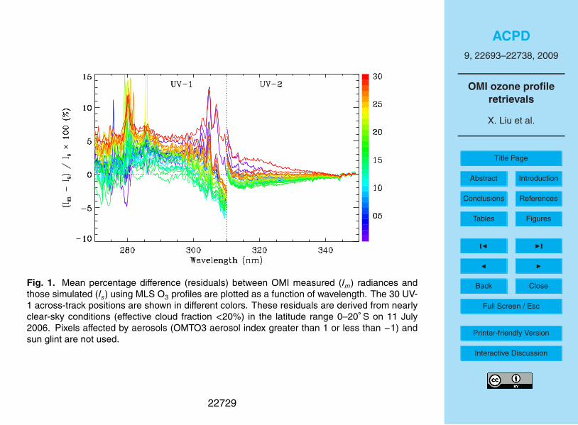
ACPD9, 22693–22738, 2009


X. Liu et al.

Title Page



Tables Figures

J I

J I

Back Close

Full Screen / Esc



Fig. 1. Mean percentage difference (residuals) between OMI measured (Im) radiances andthose simulated (Is) using MLS O3 profiles are plotted as a function of wavelength. The 30 UV-1 across-track positions are shown in different colors. These residuals are derived from nearlyclear-sky conditions (effective cloud fraction <20%) in the latitude range 0–20◦ S on 11 July2006. Pixels affected by aerosols (OMTO3 aerosol index greater than 1 or less than −1) andsun glint are not used.

22729





ACPD9, 22693–22738, 2009


X. Liu et al.

Title Page



Tables Figures

J I

J I

Back Close

Full Screen / Esc



Fig. 2. An orbit of retrievals at across-track position 16 (in the UV-1 channel) on 11 July 2006as a function of latitude, longitude, and solar zenith angle. (a) Ozone profiles in number density,and (b) the effective cloud fraction (black), fitted surface albedo (purple) for the UV-2 channel,and effective cloud-top pressure (red) used in the retrievals. The white line in (a) indicates theNCEP thermal tropopause.

22730





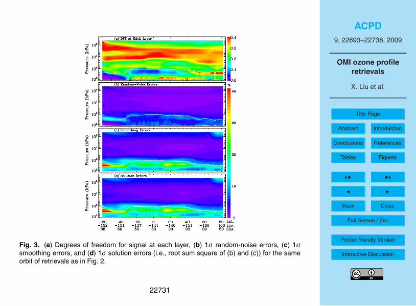
ACPD9, 22693–22738, 2009


X. Liu et al.

Title Page



Tables Figures

J I

J I

Back Close

Full Screen / Esc



38

Fig. 3. (a) Degrees of freedom for signal at each layer, (b) 1σ random-noise errors, (c) 1σ

smoothing errors, and (d) 1σ solution errors (i.e., root sum square of (b) and (c)) for the

same orbit of retrievals as in Fig. 2.

Fig. 3. (a) Degrees of freedom for signal at each layer, (b) 1σ random-noise errors, (c) 1σsmoothing errors, and (d) 1σ solution errors (i.e., root sum square of (b) and (c)) for the sameorbit of retrievals as in Fig. 2.

22731





ACPD9, 22693–22738, 2009


X. Liu et al.

Title Page



Tables Figures

J I

J I

Back Close

Full Screen / Esc



Fig. 4. (a) Total, stratospheric, and tropospheric degrees of freedom for signal, (b) 1σ random-noise errors in total, stratospheric, and tropospheric ozone columns, (c) same as (b) but for1σ smoothing errors, and (d) same as (b) but for 1σ solution errors (i.e., root sum square of(b) and (c)), for the same orbit of retrievals as in Fig. 2. The thin lines in (a) are for retrievalsunder ideal conditions (i.e., without interferences from other parameters).

22732





ACPD9, 22693–22738, 2009


X. Liu et al.

Title Page



Tables Figures

J I

J I

Back Close

Full Screen / Esc



Fig. 5. (a–c) are three examples of nearly clear-sky retrieval averaging kernels for pixels (1)–(3) indicated on Figs. 2a and 3a. (d–e) are the same as (a–c) but under ideal conditions (i.e.,without interferences from other parameters). These AKs have been normalized by the actualozone variability (i.e., a priori error) because ozone values vary by more than two orders ofmagnitude at different layers. The dotted black horizontal lines indicate the tropopause. Thecaption on top of each of panel shows solar zenith angle, cloud fraction, and surface albedo.

22733





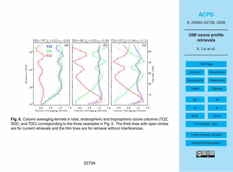
ACPD9, 22693–22738, 2009


X. Liu et al.

Title Page



Tables Figures

J I

J I

Back Close

Full Screen / Esc



Fig. 6. Column averaging kernels in total, stratospheric and tropospheric ozone columns (TOZ,SOC, and TOC) corresponding to the three examples in Fig. 5. The thick lines with open circlesare for current retrievals and the thin lines are for retrieval without interferences.

22734





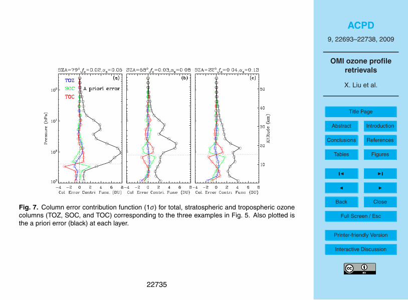
ACPD9, 22693–22738, 2009


X. Liu et al.

Title Page



Tables Figures

J I

J I

Back Close

Full Screen / Esc



Fig. 7. Column error contribution function (1σ) for total, stratospheric and tropospheric ozonecolumns (TOZ, SOC, and TOC) corresponding to the three examples in Fig. 5. Also plotted isthe a priori error (black) at each layer.

22735





ACPD9, 22693–22738, 2009


X. Liu et al.

Title Page



Tables Figures

J I

J I

Back Close

Full Screen / Esc



43

Fig. 8. Maps of total ozone column (a), stratospheric ozone column (b), tropospheric

ozone column (c), and cloud fraction (d) on 26 August 2006. The data are mapped on 1º

longitude × 1º latitude grid cells. Some systematic cross-track position dependent biases

have been removed before gridding by assuming these data do not vary with cross-track

position within a month. The black contours on (a) and (b) indicate the NCEP tropopause

pressure used (The contour levels are 100, 150, 200, 250, 300, 350 hPa) and the two

white dashed lines indicate the latitudes where zonal cross sections of tropospheric ozone

profiles are shown in Fig. 9.

Fig. 8. Maps of total ozone column (a), stratospheric ozone column (b), tropospheric ozonecolumn (c), and cloud fraction (d) on 26 August 2006. The data are mapped on 1◦ longitude×1◦ latitude grid cells. Some systematic cross-track position dependent biases have been re-moved before gridding by assuming these data do not vary with cross-track position withina month. The black contours on (a) and (b) indicate the NCEP tropopause pressure used (thecontour levels are 100, 150, 200, 250, 300, 350 hPa) and the two white dashed lines indicatethe latitudes where zonal cross sections of tropospheric ozone profiles are shown in Fig. 9.

22736





ACPD9, 22693–22738, 2009


X. Liu et al.

Title Page



Tables Figures

J I

J I

Back Close

Full Screen / Esc



Fig. 9. Longitudinal cross sections of ozone volume mixing ratio from the surface to 100 hPaat 10.5◦ S and 35.5◦ N, corresponding to the dashed white lines in Fig. 8. The retrieved partialozone columns are interpolated to a finer vertical grid and are converted to volume mixing ratio.The white lines indicate the NCEP tropopause.

22737





ACPD9, 22693–22738, 2009


X. Liu et al.

Title Page



Tables Figures

J I

J I

Back Close

Full Screen / Esc



Fig. 10. An event of transpacific transport of pollution from East Asia across the North PacificOcean to the United States on 5–9 May 2006. (a) Mean tropospheric ozone volume mixingratio, (b) longitudinal cross sections of ozone profiles below 100 hPa at 31.5◦ N and (c) sameas (b) but at 41.5◦ N. The dashed lines on (a) indicate the latitudes of cross sections. The whitelines indicate the NCEP tropopause. The data are mapped on 1◦ longitude×1◦ latitude gridcells.

22738





omi ozone profile retrievals - · acpd 9, 22693–22738, 2009 omi ozone proﬁle retrievals x. liu...

Documents