This article was downloaded by: [Texas A&M University Libraries]On: 02 September 2014, At: 12:58Publisher: Taylor & FrancisInforma Ltd Registered in England and Wales Registered Number: 1072954 Registered office: Mortimer House,37-41 Mortimer Street, London W1T 3JH, UK

Journal of the American Statistical AssociationPublication details, including instructions for authors and subscription information:http://www.tandfonline.com/loi/uasa20

Spline-Based Emulators for Radiative ShockExperiments With Measurement ErrorAvishek Chakraborty a , Bani K. Mallick a , Ryan G. Mcclarren b , Carolyn C. Kuranz b , DerekBingham c , Michael J. Grosskopf c , Erica M. Rutter c , Hayes F. Stripling c & R. Paul Drake da Department of Statistics , Texas A&M University , College Station , TX , 77843-3143b Department of Nuclear Engineering , Texas A&M University , College Station , TX ,77843-3133c Department of Atmospheric, Oceanic and Space Sciences , University of Michigan , AnnArbor , MI , 48109-2143d Department of Statistics and Actuarial Science , Simon Fraser University , Burnaby , BC ,V5A 1S6 , CanadaAccepted author version posted online: 04 Feb 2013.Published online: 01 Jul 2013.

To cite this article: Avishek Chakraborty , Bani K. Mallick , Ryan G. Mcclarren , Carolyn C. Kuranz , Derek Bingham ,Michael J. Grosskopf , Erica M. Rutter , Hayes F. Stripling & R. Paul Drake (2013) Spline-Based Emulators for RadiativeShock Experiments With Measurement Error, Journal of the American Statistical Association, 108:502, 411-428, DOI:10.1080/01621459.2013.770688

To link to this article: http://dx.doi.org/10.1080/01621459.2013.770688

PLEASE SCROLL DOWN FOR ARTICLE

Taylor & Francis makes every effort to ensure the accuracy of all the information (the “Content”) containedin the publications on our platform. However, Taylor & Francis, our agents, and our licensors make norepresentations or warranties whatsoever as to the accuracy, completeness, or suitability for any purpose of theContent. Any opinions and views expressed in this publication are the opinions and views of the authors, andare not the views of or endorsed by Taylor & Francis. The accuracy of the Content should not be relied upon andshould be independently verified with primary sources of information. Taylor and Francis shall not be liable forany losses, actions, claims, proceedings, demands, costs, expenses, damages, and other liabilities whatsoeveror howsoever caused arising directly or indirectly in connection with, in relation to or arising out of the use ofthe Content.

This article may be used for research, teaching, and private study purposes. Any substantial or systematicreproduction, redistribution, reselling, loan, sub-licensing, systematic supply, or distribution in anyform to anyone is expressly forbidden. Terms & Conditions of access and use can be found at http://www.tandfonline.com/page/terms-and-conditions

Supplementary materials for this article are available online. Please go to www.tandfonline.com/r/JASA

Spline-Based Emulators for Radiative ShockExperiments With Measurement Error

Avishek CHAKRABORTY, Bani K. MALLICK, Ryan G. MCCLARREN, Carolyn C. KURANZ, Derek BINGHAM,Michael J. GROSSKOPF, Erica M. RUTTER, Hayes F. STRIPLING, and R. Paul DRAKE

Radiation hydrodynamics and radiative shocks are of fundamental interest in the high-energy-density physics research due to their importancein understanding astrophysical phenomena such as supernovae. In the laboratory, experiments can produce shocks with fundamentally similarphysics on reduced scales. However, the cost and time constraints of the experiment necessitate use of a computer algorithm to generate areasonable number of outputs for making valid inference. We focus on modeling emulators that can efficiently assimilate these two sources ofinformation accounting for their intrinsic differences. The goal is to learn how to predict the breakout time of the shock given the informationon associated parameters such as pressure and energy. Under the framework of the Kennedy–O’Hagan model, we introduce an emulatorbased on adaptive splines. Depending on the preference of having an interpolator for the computer code output or a computationally fastmodel, a couple of different variants are proposed. Those choices are shown to perform better than the conventional Gaussian-process-basedemulator and a few other choices of nonstationary models. For the shock experiment dataset, a number of features related to computermodel validation such as using interpolator, necessity of discrepancy function, or accounting for experimental heterogeneity are discussed,implemented, and validated for the current dataset. In addition to the typical Gaussian measurement error for real data, we consider alternativespecifications suitable to incorporate noninformativeness in error distributions, more in agreement with the current experiment. Comparativediagnostics, to highlight the effect of measurement error model on predictive uncertainty, are also presented. Supplementary materials forthis article are available online.

KEY WORDS: Adaptive spline; Computer model validation; Emulator; Measurement error model; Non-Gaussian error; Reversible jumpMarkov chain Monte Carlo.

1. INTRODUCTION

High-energy density physics (HEDP) studies the behavior ofsystems with a pressure at or above 1 million times atmosphericpressure (Drake 2006). Such high-energy-density systems oc-cur in astrophysical phenomena [e.g., supernovae explosions(Chevalier 1997)]. Given advances in laser technology, the high-energy-density regime is now routinely accessible in laboratoryexperiments where a laser focused on a target accelerates ma-terial to create shock waves of about 10 kilometers per second.Shock waves traveling at these extreme speeds radiate light in theX-ray spectrum (as a result of black-body radiation emission)that fundamentally alters the propagation of the shock whencompared with traditional shocks such as the shock wave cre-ated by supersonic aircraft. These shocks are said to be radiativeshocks and described by the radiation-hydrodynamics physicsmodel comprised of traditional hydrodynamics augmented withequations that govern the transport of radiation.

Avishek Chakraborty is Postdoctoral Associate (E-mail: avishekc@stat.tamu.edu) and Bani Mallick is Distinguished Professor (E-mail:bmallick@stat.tamu.edu) in the Department of Statistics, Texas A&M Univer-sity, College Station, TX 77843-3143. Ryan G. McClarren is Assistant Profes-sor (E-mail: rgm@tamu.edu) and Hayes F. Stripling is Ph.D. candidate (E-mail:h.stripling@tamu.edu) in the Department of Nuclear Engineering, Texas A&MUniversity, College Station, TX 77843-3133. Carolyn C. Kuranz is AssistantResearch Scientist (E-mail: ckuranz@umich.edu), Michael J. Grosskopf is Re-search Engineer (E-mail: mikegros@umich.edu), Erica M. Rutter is a ResearchTechnician (E-mail: ruttere@umich.edu), and R. Paul Drake is Henry SmithCarhart Professor of Space Science (E-mail: rpdrake@umich.edu) in the De-partment of Atmospheric, Oceanic and Space Sciences, University of Michigan,Ann Arbor, MI 48109-2143. Derek Bingham is Associate Professor in the De-partment of Statistics and Actuarial Science, Simon Fraser University, Burnaby,BC V5A 1S6, Canada (E-mail: dbingham@stat.sfu.ca). This work was fundedby the Predictive Sciences Academic Alliances Program in DOE/NNSA-ASCvia grant DEFC52- 08NA28616. The authors thank the editors and referees fortheir insightful feedback and for helping to improve the content and presentationof this article.

Using the Omega Laser Facility at Rochester University(Boehly et al. 1995), several experimental campaigns have beenconducting HEDP experiments concerned with understandingradiative shocks. In these experiments, a disk of beryllium(atomic symbol Be) is placed at the end of a plastic tube ofxenon (atomic symbol Xe). Then the laser is discharged ontothe Be disk; the energy deposition of the laser causes a layerof Be to ablate thereby accelerating a shock into the Be. Thisshock travels through the Be and “breaks out” of the disk intothe Xe gas where radiography is able to capture images of theshock structure. These experiments require the dedication oflarge amounts of resources in terms of laser time, fabricationcosts, and experimentalist time and, as a result, only tens ofsuch experiments are performed per year. Hence, to deal withthe scarcity of experimental data, it is natural to turn to computersimulation to understand the behavior of the radiating shocks inthe experiment and to predict the results of new experiments.The fidelity of the simulation must, nevertheless, be validatedwith experimental data, and therefore, our interest lies in assim-ilating the information obtained from these simulator runs andfield experiments. In the present literature, we often have similarsituations where computer algorithms or numerical proceduresare designed to describe or closely approximate a real-life ex-periment or physical process. Examples arise in diverse areas ofscience including cosmic mass distribution (Habib et al. 2007),heat transfer (Higdon et al. 2008b), volcano analysis (Bayarriet al. 2009), atmospheric sciences (Kennedy et al. 2008),and hydrodynamics (Williams et al. 2006). Accuracy of theexperimental data can be quantified in some of these cases (asours, see Section 2), but all inputs to the experimental system

© 2013 American Statistical AssociationJournal of the American Statistical Association

June 2013, Vol. 108, No. 502, Applications and Case StudiesDOI: 10.1080/01621459.2013.770688

411

Dow

nloa

ded

by [

Tex

as A

&M

Uni

vers

ity L

ibra

ries

] at

12:

58 0

2 Se

ptem

ber

2014

412 Journal of the American Statistical Association, June 2013

cannot be controlled or even measured. Thus, the main chal-lenge in this regime is to account for the uncertainty due to theunknown state of the natural parameters that influence outcomeof the experiment. However, for the simulator, all the factorsthat are believed to be influential in determining the responseare provided as controlled input to the code. Also the mathemat-ical model used for the simulation may only partially representthe true physical process, leading to discrepancy between ex-perimental and simulator outputs. These simulators themselvesoften represent complex mathematical models and can be ex-pensive to run in terms of cost and time. An emulator is astochastic surrogate for the simulator; it is fast to implementand enables the user to predict a large number of code outputsas desired input configurations. The main task of the emulator isto learn the relationship between inputs and response from thecode results and then to use it for calibration of the unknownparameters of the real-world process by matching it with corre-sponding responses. This enables both (i) running the simulatorwith input configuration that resembles the real-world param-eters better and (ii) predicting the outcome of a real-life eventwith knowledge of only a subset of the inputs.

The basic statistical framework for validating computer mod-els was developed in the recent literature. Sacks, Schiller,and Welch (1989) used the Gaussian process (GP) as themodel deterministic computer codes to obtain uncertainty es-timates at untried input configurations. Later, Kennedy andO’Hagan (2001) built a joint model (referred to henceforth asthe Kennedy–O’Hagan model) for the experimental data andthe code output. Their model uses a GP prior for the emula-tor and, in a hierarchical structure, efficiently assimilates thetwo sources of information accounting for their intrinsic differ-ences. In a similar setup, Higdon et al. (2004) discussed un-certainty quantification and potential discrepancy between thephysical model and the real-world system. Of late, extensionof the Kennedy–O’Hagan model to multivariate (and possiblyhigh dimensional) outputs has been developed in Higdon et al.(2008a). For other works in this field, covering a wide rangeof applications and extensions, see, for example, Bayarri et al.(2007), Liu and West (2009), Fricker, Oakley, and Urban (2010),Bastos and OHagan (2009), and references therein. While ma-jority of the literature uses GP emulators, here we propose twoalternative specifications based on splines. Splines are commonin regression problems (Smith and Kohn 1998; Denison et al.2002). In Section 3.2, we argue about their advantages over GP,and in Section 5, we provide diagnostic results from the dataanalysis in favor of them.

Another area of focus in this article is to construct an appropri-ate model for measurement error associated with the experimen-tal output. The measurement error is universal to almost everydata collection procedure. Early work with the measurementerror in a generalized linear model can be found in Stefanskiand Carroll (1987). Mallick and Gelfand (1995) developed aBayesian approach for this problem relating the data, parame-ters, and unmeasured variables through a hierarchical structure.A Gaussian distribution is the usual choice for noise modeling.However, it may not be robust in every situation, specifically, inthe examples where the error is known to have a skewed or flat-shaped structure. Non-Gaussian or skewed error specificationswere used by Chen, Gott, and Ratra (2003), Arellano-Valle et al.

(2005), and Rodrigues and Bolfarine (2007). In Section 4, wediscuss two alternative ways to combine multiple sources of er-ror, accounting for potential noninformativeness. Comparativeperformance analysis against the Gaussian error specification,based on experimental data, is provided in Section 5.

The article is organized as follows. Section 2 describes theexperiment and the associated simulator in detail. In Section 3,within the generic formulation of the full hierarchical model,multiple alternative specifications are suggested, discussed andcompared against each other. Section 4 extends this model withnon-Gaussian error proposals for field experiments. In Section5, we present an in-depth analysis of the shock experimentdataset. Finally, in Section 6, along with a summary of ourwork, additional possibilities for improvement, in the context ofthe current problem as well as the general modeling in this area,are outlined as topics of future research.

2. DETAILS OF SHOCK EXPERIMENT

Let us start with the motivation for studying shock featuresin physics. Subsequently we discuss the details of the labora-tory experiment as well as the associated simulator, developedby the Center for Radiating Shock Hydrodynamics (CRASH;http://aoss-research.engin.umich.edu/crash/ ), funded by theDepartment of Energy Predictive Science Academic AllianceProgram (PSAAP).

2.1 Scientific Relevance

Radiative shocks are of significant interest to researchers dueto their connection to astrophysical shocks. In any shock wave,heating at the shock transition leads to heating and compressionof the matter entering the shock. If the shock wave is strongenough, the heating becomes so large that radiation from theheated matter carries a significant amount of energy upstream(because light travels faster than the shock wave) and, as a result,alters the unshocked material and, therefore, the structure of theshock. Such shocks are called radiative shocks, and in theseshocks, the transport of radiative energy plays an essential rolein the dynamics. In astrophysics, systems with large velocitiesor very hot interiors are common, so radiative shocks are ubiq-uitous. Moreover, the shock waves emerging from supernovaeand the shock waves that can be produced in laboratory exper-iments have specific similarities such as the optical depth (theratio of the average distance the radiation travels before beingabsorbed to the length of the system) and the shock strength,which relates the shock speed to the thermodynamic propertiesof the material.

2.2 Experimental Details

In the laboratory experiment, first a laser pulse irradiates athin disk of Be metal at the end of a tube of Xe, as in Figure 1.The energy of the laser causes the surface of the Be to ablate.To balance the momentum of the ablating material, a shockwave is driven into the Be at about 50 km/s. When this shockwave breaks out of the Be into the Xe, it is propagating at aspeed of roughly 200 km/s and heats the Xe to temperaturesabove 5 × 105 K. At these high temperatures, the Xe becomes aplasma and emits a great deal of energy in the form of soft X-ray

Dow

nloa

ded

by [

Tex

as A

&M

Uni

vers

ity L

ibra

ries

] at

12:

58 0

2 Se

ptem

ber

2014

Chakraborty et al.: Radiative Shock Experiments 413

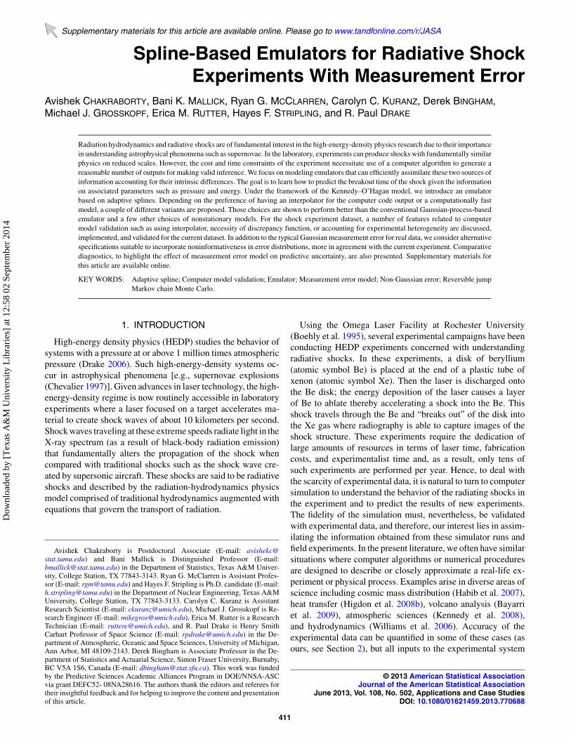
Figure 1. The Be disk is irradiated with several laser beams to drivea radiative shock in the tube of Xe gas. The main diagnostic for theradiative shock experiment is X-ray radiography. This technique isexecuted by additional laser beams irradiating a metal foil to createX-ray photons that pass through the target to an X-ray detector. Theonline version of this figure is in color.

radiation. This radiation travels ahead of the shock, heating theunshocked Xe and providing feedback to the shock dynamics.

In October 2008, a set of radiative shock experiments wereconducted at the Omega laser. There were a number of con-trolling factors such as Be drive disk thickness, laser energy,Xe pressure, and observation time, which were varied from oneexperiment to another. Outcomes of interest were the shock fea-tures such as its position down the tube, time of breakout fromthe Be disk, and its speed. Measurement of these outcomes in-volved multiple sources of error. Specifically the shock breakouttime, the feature of interest in this article, was measured usingthree different instruments of varying accuracy ranging from 10to 30 picoseconds (ps). Two of them were velocity interferom-

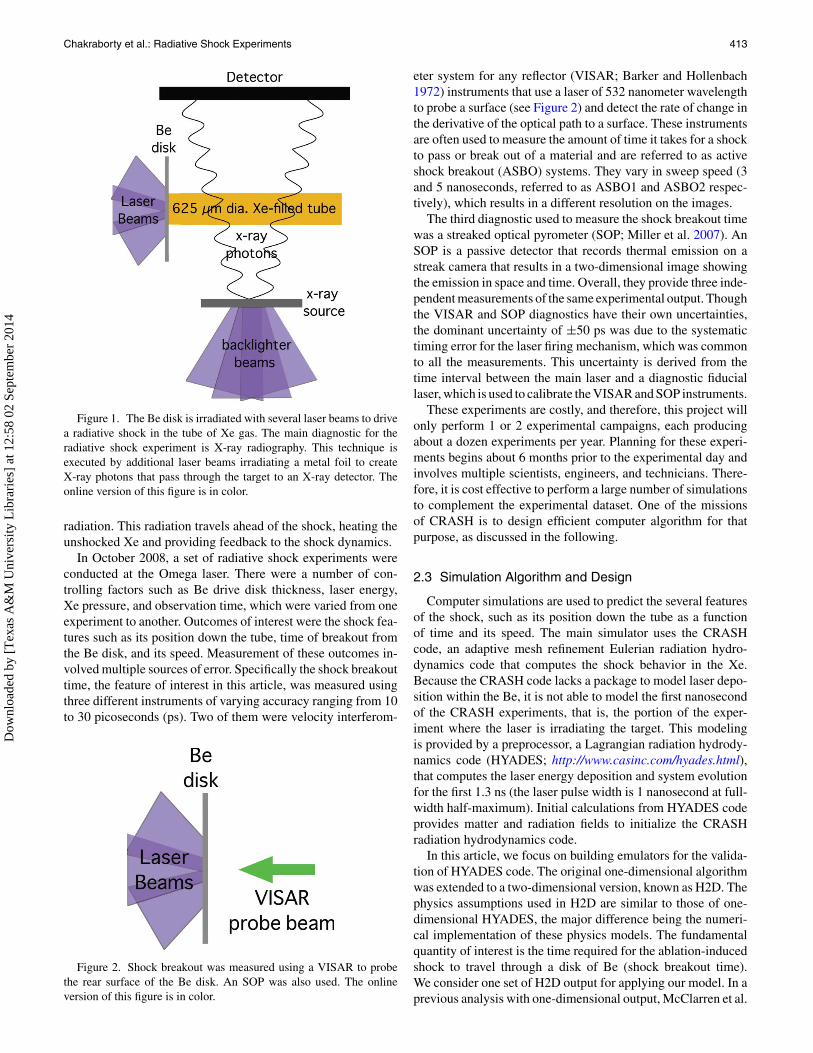
Figure 2. Shock breakout was measured using a VISAR to probethe rear surface of the Be disk. An SOP was also used. The onlineversion of this figure is in color.

eter system for any reflector (VISAR; Barker and Hollenbach1972) instruments that use a laser of 532 nanometer wavelengthto probe a surface (see Figure 2) and detect the rate of change inthe derivative of the optical path to a surface. These instrumentsare often used to measure the amount of time it takes for a shockto pass or break out of a material and are referred to as activeshock breakout (ASBO) systems. They vary in sweep speed (3and 5 nanoseconds, referred to as ASBO1 and ASBO2 respec-tively), which results in a different resolution on the images.

The third diagnostic used to measure the shock breakout timewas a streaked optical pyrometer (SOP; Miller et al. 2007). AnSOP is a passive detector that records thermal emission on astreak camera that results in a two-dimensional image showingthe emission in space and time. Overall, they provide three inde-pendent measurements of the same experimental output. Thoughthe VISAR and SOP diagnostics have their own uncertainties,the dominant uncertainty of ±50 ps was due to the systematictiming error for the laser firing mechanism, which was commonto all the measurements. This uncertainty is derived from thetime interval between the main laser and a diagnostic fiduciallaser, which is used to calibrate the VISAR and SOP instruments.

These experiments are costly, and therefore, this project willonly perform 1 or 2 experimental campaigns, each producingabout a dozen experiments per year. Planning for these experi-ments begins about 6 months prior to the experimental day andinvolves multiple scientists, engineers, and technicians. There-fore, it is cost effective to perform a large number of simulationsto complement the experimental dataset. One of the missionsof CRASH is to design efficient computer algorithm for thatpurpose, as discussed in the following.

2.3 Simulation Algorithm and Design

Computer simulations are used to predict the several featuresof the shock, such as its position down the tube as a functionof time and its speed. The main simulator uses the CRASHcode, an adaptive mesh refinement Eulerian radiation hydro-dynamics code that computes the shock behavior in the Xe.Because the CRASH code lacks a package to model laser depo-sition within the Be, it is not able to model the first nanosecondof the CRASH experiments, that is, the portion of the exper-iment where the laser is irradiating the target. This modelingis provided by a preprocessor, a Lagrangian radiation hydrody-namics code (HYADES; http://www.casinc.com/hyades.html),that computes the laser energy deposition and system evolutionfor the first 1.3 ns (the laser pulse width is 1 nanosecond at full-width half-maximum). Initial calculations from HYADES codeprovides matter and radiation fields to initialize the CRASHradiation hydrodynamics code.

In this article, we focus on building emulators for the valida-tion of HYADES code. The original one-dimensional algorithmwas extended to a two-dimensional version, known as H2D. Thephysics assumptions used in H2D are similar to those of one-dimensional HYADES, the major difference being the numeri-cal implementation of these physics models. The fundamentalquantity of interest is the time required for the ablation-inducedshock to travel through a disk of Be (shock breakout time).We consider one set of H2D output for applying our model. In aprevious analysis with one-dimensional output, McClarren et al.

Dow

nloa

ded

by [

Tex

as A

&M

Uni

vers

ity L

ibra

ries

] at

12:

58 0

2 Se

ptem

ber

2014

414 Journal of the American Statistical Association, June 2013

(2011) found only five of the inputs to have significant effecton the response: Be disk thickness, laser energy, electron fluxlimiter (related to heat transport by the electrons), Be gammaconstant (related to the compressibility of Be), and the compu-tational mesh resolution in the Be. Later, the mesh resolutionwas fixed keeping in mind code stability and convergence andwas used for all subsequent runs of HYADES. Along with theprevious four parameters, an additional source of uncertaintyspecifically for the two-dimensional solution was the wall opac-ity of the plastic tube, which controls how strongly radiation isabsorbed.

To construct a fast running preprocessor, a set of 104 runswas conducted to cover this five-dimensional input space. Thechoice of these input settings (i.e., the experimental design) wasa combination of a smaller space filling Latin hypercube design,with additional points added according to a space-filling crite-rion. More specifically, the first 64 design points, or runs, werechosen using an orthogonal array-based Latin hypercube design(LHD) Tang (1993). The base orthogonal array was a repli-cated 25 factorial design, and these points converted to a Latinhypercube. The orthogonal array-based design guarantees thatthe cells (or strata) defined by the factorial design contain thesame number of points and the space filling criterion aims to fillthe input space as uniformly as possible. Since the constructionof such designs involves random permutations, there are manypossible designs that can be constructed in this manner. So, toidentify a very good one, many designs were generated and theone that optimized the so-called maximin space filling criterion[maximizing the minimum distance between design points, seeJohnson, Moore, and Ylvisaker (1990)] was chosen. Next, abatch of 10 new design points was added to the existing 64 rundesign. The points were allocated so that the maximin criterionwas again optimized, conditional on the first set of the points.The procedure of adding 10 points at a time was repeated until atotal of 104 design points were identified. The design was con-structed in this way since it was not clear from the start whetherit would be possible to complete 104 runs with the availablefinancial resources. Therefore, if this limit got exceeded in anyintermediate step between 64 and 104 trials, the resulting designwould still have very good space filling properties. The analysisof this dataset is presented in Section 5.

3. HIERARCHICAL MODEL

We start with a description of the basic framework for acomputer code validation problem, based on the specificationin Kennedy and O’Hagan (2001). Under this setup, we builda multistage model for joint analysis of the experimental andsimulation outputs. A variety of competing model choices areproposed for the emulator. We discuss their properties, limi-tations, and mutual differences. Finally, we provide details ofestimation procedure.

3.1 Generic Hierarchical Specification

Suppose we have obtained data from n runs of the simula-tor and m trials of the experiment. Denote by y

(r)i , y

(c)i the ith

response from the experiment and the simulator, respectively;x

(r)i , x

(c)i denote corresponding p-dimensional inputs known un-

der both scenarios; θ (r) denotes the q-dimensional vector of

unobserved natural parameters that is believed to have an influ-ence on the response. The simulator is run at n different knowncombinations θ

(c)1 , θ

(c)2 , . . . , θ (c)

n of these parameters. Usually,the combinations are chosen using a prior knowledge aboutrange and likely values of the features.

We introduce the multistage model in an incremental manner.Whenever possible, we omit the subscripts indexing the datapoints. In the first stage, we specify a stochastic model MC forthe simulator as

MC : y(c) = f (x(c), θ (c)) + ηc(x(c), θ (c)). (1)

Next, MC is hierarchically related to the model for the experi-ments MR as

MR : y(r) = f (x(r), θ (r)) + δr (x(r)). (2)

In the above equation, f is the link function between the codeand the experiment, which captures the major patterns commonto both of them; ηc and δr represent their individual residualpatterns. In practice, the experiment and the simulation havetheir own biases and uncertainties. Physical models often in-volve complex optimizations or set of equations that do notadmit closed-form solutions, but require use of numerical al-gorithms. Irrespective of how the observations are simulated,any such code output is likely to have an associated uncertaintyfrom multiple perspectives such as sensitivity to the choice ofinitial value, simplifying assumptions, prespecified criterion forconvergence, etc. Similarly, the input–output relationship in anactual event can deviate from the theoretical prediction due tomany reasons such as input uncertainty, lack of knowledge aboutpossible factors (other than θ ) influencing the experimental out-come, and, more importantly, partial accuracy of the mathemat-ical model. Hence, we account for them with the inclusion of ηc

and δr in MC and MR , respectively. The focus of this articleis to propose and compare different model specifications for f .We defer that entirely to Section 3.2.

The above interpretation relies on the specification of f andδr . From the modeling perspective, (1) and (2) represent two re-gression problems. A priori, we believe that the solution of themathematical model is a good approximation of the experimen-tal outcome, that is, the two response functions are expected tomatch. Accordingly, f can be seen as the shared mean surfaceand δr and ηc as zero-mean residual processes for the experimentand the simulator, respectively. As usual for any regression prob-lem, the properties of the residuals depend on the specificationof mean, for example, using a linear mean for a quadratic re-sponse function can produce heteroscedastic residuals, whereaschoosing a second-order mean may lead to homoscedastic pat-tern. Hence, if f is constrained to have a fixed functional form oris chosen from a fixed family of functions, interpretation of theestimates of the residuals (ηc and δr ) is subject to that selection.However, for the purpose of this problem, learning of the indi-vidual functions is not the primary goal of inference; the objec-tive is to improve predictions from these models. The functionsf, ηc, and δr serve as tools for that. Using the stochastic model,we want to predict the outcome, with reasonable accuracy, at anuntried input configuration without the need to perform com-plex simulations (and even more expensive experiments) in thelong run. Hence, we want f and δr to be flexible enough sothat, through MC and MR , we can efficiently approximate the

Dow

nloa

ded

by [

Tex

as A

&M

Uni

vers

ity L

ibra

ries

] at

12:

58 0

2 Se

ptem

ber

2014

Chakraborty et al.: Radiative Shock Experiments 415

Figure 3. Graphical model for the experimental system: the con-trolled inputs x(r) and natural parameters θ (r) influence the emulatorf . Generation of the actual outcome y(r) also involves additional biasthrough input-dependent bias δ(·) and pure error τ (r). Three devices,all sharing a common bias ε0 but different device-specific biases εj ,are used to produce measurements y

(o)j , j = 1, 2, 3, separately, of the

same experimental outcome.

response functions of the simulator and the experimental sys-tem, respectively. Reasonable and well-defined specificationsfor f are subject to user judgment and practical considerations.As a simple example, we may decide to include polynomialsonly upto a certain order in the emulator specification. Whenηc ≡ 0, we get back the usual Kennedy–O’Hagan specificationwith f as an interpolator for the computer output and δr as dis-crepancy capturing the potential inadequacy of the mathematicalmodel to explain the dynamics of an actual experiment.

We return to the model. For modeling the residual process δr

in MR , we decompose it into a zero-mean covariate-dependentrandom effect plus a nugget, similar to a spatial regression model(Banerjee, Carlin, and Gelfand 2004):

δr

(x(r)

) = δ(x(r)

)+ τ (r).

In the literature, δ(·) is modeled using a GP on x(r) (Higdonet al. 2004); τ (r) accounts for variation in repeated experimentswith identical x(r) due to the factors that were unobserved andunaccounted for in the model.

Although y(r) is the actual outcome of the real-world experi-ment, usually it is measured with some error. Specifically, for thecurrent dataset, three different procedures were used to measurethe output of each experiment with different degrees of accuracy(known a priori). There was also a common measurement errorε0 of known scale, see Section 2.2. Hence, we augment a thirdstage to the hierarchy: the measurement error model ME forthe observed output y(o) conditional on y(r) as follows:

ME : y(o)j = y(r) + εj + ε0 ; j = 1, 2, 3, (3)

where εj is the error specific to measurement procedure j. MR

and ME can be simultaneously represented through Figure 3.

3.2 Choice of Functions With Interpretation

In scientific experiments, it is often desirable to use a spec-ification for MC , that is, an interpolator. For code outputs ofdeterministic nature (i.e., different simulator runs with same in-put combination produce the exact same output), one expectsthe stochastic model to exactly fit the observed responses atthe corresponding input levels. GP is an interpolator, but usingany other residual distribution inside MC (such as white noise

(WN) or heteroscedastic but independent residuals) violates thatcondition.

By definition, an emulator is a stochastic substitute of thesimulator and should be easy to run than the latter. Thus, it shouldbe computationally robust with respect to the size of simulationdataset. For the shock experiment dataset, the H2D simulator isless expensive to run than the corresponding field experiment,hence over time it is possible to conduct more and more trials. Ingeneral, regression with independent errors are computationallyconvenient than GP regression where the inversion of covariancematrix gets increasingly complicated as n increases.

Next, we mention some possible choices for f and comparethem on the basis of above criteria:

• GP emulator: The original Kennedy–O’Hagan specifica-tion Kennedy and O’Hagan (2001) used a GP prior for theemulator f . GP is by now common in nonparametric Bayesliterature as prior for regression functions (Neal 1999; Shiand Choi 2011) and in geostatistics to model the responsecorrelated over space (Banerjee, Carlin, and Gelfand 2004).The model is specified as

f (·) ∼ GP(μ(·), C(·, ·)), ηc(·) = 0. (4)

The mean function μ(·) can be chosen as a polynomial in(x, θ ) and the covariance function C(·, ·) is often speci-fied to have a stationary correlation structure along with aconstant scale, that is, if a = (x1, θ1), b = (x2, θ2) are twoinputs to the simulator, then

Ca,b(σ 2, ν) = σ 2p+q∏s=1

κ(|as − bs |, νs),

where κ is a valid correlation function on R and νs is the pa-rameter specific to sth input. Together, forms of κ and {νs}control the correlation (hence smoothness) in the emulatorsurface over the input space. Choice for κ is welldiscussedin literature, the most popular being the Matern familyof functions Matern (1960), for example, exponential andGaussian correlation functions.

The specification in (4) makes f as well as MC inter-polators for the simulator outputs. The computation forthe parameters of f are fairly standard, but with a largenumber of sample points, inversion of the sample covari-ance matrix gets difficult. Several approximation methodsare available in that case including process convolution(Higdon 2002), approximate likelihood (Stein, Chi, andWelty 2004), fixed rank kriging (Cressie and Johannes-son 2008), covariance tapering (Kaufman, Schervish, andNychka 2008), predictive process (Banerjee et al. 2008),and compactly supported correlation functions (Kaufmanet al. 2011).

• A spline-based alternative: As discussed earlier, we want fto be robust to the possibility of overfitting the simulationdataset. The emulator f should have a strong predictiveproperty for experiments with new sets of inputs. In thatregard, using a model that fits exactly the code samplesmay not be desirable. The complexity of the physics aswell as numerical approximation to solve the computermodel makes it unlikely to develop codes that can fullysimulate the experiments. Also computational efficiency

Dow

nloa

ded

by [

Tex

as A

&M

Uni

vers

ity L

ibra

ries

] at

12:

58 0

2 Se

ptem

ber

2014

416 Journal of the American Statistical Association, June 2013

in estimating parameters of f is desirable. Specifying f assum of local interactions of varying order using a completeclass of basis functions serves these needs and providesgreater flexibility to model relationships among variables.A number of options are available, including multivari-ate adaptive regression splines (MARS; Friedman 1991;Denison, Mallick, and Smith 1998) as

f (x) =k∑

h=1

βhφh(x), ηc(x) ind noise,

φ1(x) = 1; φh(x) =nh∏l=1

[uhl

(xvhl

− thl

)]+ ; h > 1, (5)

where (·)+ = max(·, 0) and nh is the degree of the interac-tion of basis function φh. The sign indicators {uhl} are ±1,vhl gives the index of the predictor variable that is beingsplit at the knot point thl within its range. The set {φh(·)}hdefines an adaptive partitioning of the multidimensionalpredictor space; {βh} represents the vector of weights as-sociated with the functions. The response is modeled tohave a mean f and a WN term ηc, which averages out anyadditional pattern present in the data that is not accountedfor by the components of f . For the rest of this article, werefer to this model as MARS+WN.

It is evident from the above specification that how wellf can capture the local patterns present in the response de-pends on two factors: (i) the number and positions of theknots and (ii) class of polynomials associated with eachknot. The larger number of knots implies a finer partitionof the predictor space so that we have greater flexibility inf at the expense of reduced smoothness. Also, if we allowpolynomials and interactions of all possible order, that con-stitutes a complete class of functions. Consequently, thelikelihood of observed data increases as more and moreof this type of local polynomials enter the model. Thatreduces the estimation bias but increases predictive un-certainty. Hence, to preserve the flexibility of the modelallowing for adaptive selection of its parameters, we needrestrictions that discourage such overfitting.

For choosing the number of knots in a penalized splineregression, a generalized cross-validation technique is pre-sented in Ruppert (2002). The recent work of Kauermannand Opsomer (2011) uses a maximum-likelihood-based al-gorithm for this. In both of them, penalty is introduced inthe form of a smoothing parameter attached to the weights.In our hierarchical approach, this is equivalent to usinga precision parameter in the prior for {βh}. Additionally,instead of determining the number of knots from an op-timization algorithm, we adopt a fully model-based ap-proach. Total number of knots in f is given by

∑kh=2 nh.

First, we restrict the class of polynomials that can ap-pear in φh, that is, we may set nh = 1 to include onlypiecewise linear terms and no interaction among variablesat all; nh ≤ 2 ensures that interactions (of only first orderin each participating variable) are allowed. Higher the al-lowed threshold for nh is, smoother are the basis functions{φh}. One may like to use a prior on the class of functions,so that functions of higher order (large nh) are less likely to

be chosen. Also important is to penalize large values of thenumber of basis functions k, which, in combination with{nh}, discourages presence of too many knots inside f . Weuse a Poisson prior distribution for k to assign low proba-bilities to its high values. A more stringent form of penaltyis enforced by letting the prior to be truncated at right atsome prespecified value k0, which essentially serves as themaximum number of basis functions that can be present in-side f at a time. Friedman (1991) described an alternativeapproach for limiting the number of knots by constrainingthem to be apart by at least a certain distance (in termsof number of data points between them). For computermodel-based validation problems, sometimes we can onlyhave a limited number of simulator runs available, that is,n is small. There, it may be appropriate to opt for a sparsestructure in f —using a simpler class of polynomials as wellas a smaller k0 to truncate the number of parameters en-tering the model. Treating the knots as parameters allowsthe model to locally adjust the smoothness of the fittedfunction as required, further encouraging sparsity withoutcompromising the fit.

The above specification has an advantage over the tradi-tional GP emulator in (4) in several aspects. First, the em-ulator is modeled as a sum of localized interactions allow-ing for nonstationarity. Kennedy and O’Hagan (2001) alsomentioned the need to consider such local structures in thespecification of emulator, which cannot be achieved witha stationary GP. One can attempt to use kernel-weightedmixture of stationary GPs, but computational efficiency ofthose type of models is still arguable. The flexibility ofMARS lies in the fact that the interaction functions canbe constructed adaptively, that is, the order of interaction,knot locations, signs, and even the number of such termsis decided by the pattern of the data during model-fitting,eliminating the need for any prior ad hoc or empirical judg-ment. In spite of having a flexible mean structure, MARSis easy to fit. For GP, even when stationarity holds, thecovariance specification makes it computationally incon-venient for handling large number of simulator runs. Thecomputation gets more complicated if one tries to introducenonstationarity within covariance structure. However, un-like GP, MARS with independent noise does not have theinterpolating property. If that is a constraint, we suggestmodifying (5) as follows.

• A combined approach: If we want to retain the flexibilityof f from (5) while enforcing the interpolating property onMC , we can combine the earlier specifications as

f (·) =∑

h

βhφh(·) + GP(0, C(·, ·)), ηc(·) = 0, (6)

where φh(·) is from (5). In the subsequent discussion anddata analysis, we refer to the above model as MARS+GP.Essentially, we are modeling the simulator output as a sumof two parts—a combination of local patterns of up to acertain order plus a residual pattern with a global station-ary correlation structure. This makes MC an interpolator.Choosing μ(·) = ∑

i βiφi(·) makes (4) and (6) identical.Hence, with an increase in simulator runs, (6) gets compu-tationally as difficult to fit as (4) due to the problem with

Dow

nloa

ded

by [

Tex

as A

&M

Uni

vers

ity L

ibra

ries

] at

12:

58 0

2 Se

ptem

ber

2014

Chakraborty et al.: Radiative Shock Experiments 417

associated GP, discussed earlier. In Section 5.1, we outlinea possible modification in the form of correlation functionC to handle those situations more efficiently.

3.3 Estimation and Inference From the Joint Model

Now, we discuss how to make inference from the hierar-chical model specified in Section 3.1. For the most exhaustivesampling scheme, below we choose MARS+GP as the specifi-cation for MC . With either of GP or MARS+WN as the choice,the corresponding steps can be reworked following this.

The model-fitting procedure used here is a Markov chainMonte Carlo (MCMC) scheme. The available data are(y(c)

l , x(c)l , θ

(c)l ), l = 1, 2, . . . , n and (y(r)

ij , x(r)ij ), j = 1, 2, 3, i =

1, 2, . . . , m. The set of parameters consists of the ones appear-ing in the distributions for f, ηc, δ, and τ (r) as well as θ (r). Weprovide the full model specification below.

y(o)ij = y

(r)i + εi0 + εij ; j = 1, 2, 3,

y(r)i = f

(x

(r)i , θ (r))+ δ

(x

(r)i

)+ τ(r)i ; i = 1, 2, . . . , m,

y(c)l = f

(x

(c)l , θ

(c)l

)+ ηc

(x

(c)l , θ

(c)l

), l = 1, 2, . . . , n,

f (x, θ ) =k∑

h=1

βhφh(x, θ ) + GP(0, C(σ 2, ν))

δ(x

(r)1:m

)∼ MVNm

(0m,C

(σ 2

δ , νδ

)), τ

(r)i

ind∼ N(0, τ 2),

εi0ind∼ N

(0, σ 2

0

); εij

ind∼ N(0, σ 2

j

),

π (β, k) ∝ MVNk

(0, σ 2

βIk

) × Pois(k − 1|λ)I (k ≤ k0). (7)

In the above equation, we use the customary additive Gaus-sian structure to combine both sources of measurement error.Alternative choices of noise distributions are discussed in Sec-tion 4. We note that, unless informative prior distributions arechosen for the scales of εj , ε0, scale of τ (r) is not identifiable(evident if we marginalize out y(r)). Since, for the shock exper-iment data, the scale of accuracy of all the measuring devicesare known beforehand, {σ 2

j : j = 0, . . . , 3} are fixed a prioriin (7). In more general applications, one must use informativepriors for each of them. Such priors can be constructed fromthe knowledge of the procedure as well as other studies wherethey have been used. As far as choice of priors is concerned,for spatial correlation in ηc and δ, we used exponential correla-tion functions. Corresponding spatial decay parameters (ν, νδ)are chosen uniformly from the interval that corresponds to areasonable spatial range in the input space. Following the dis-cussion on controlling the possibility of overfitting in MARS,(k − 1) is given a Poisson (λ) prior truncated below k0, depend-ing on the maximum number of nonconstant basis functionswe want to allow in the emulator specification. Finally, for thecalibration parameter θ (r), scientists often have a priori knowl-edge about the range of values it might have. Such knowledgemay be derived from physical understanding of the parameteror any previous study involving θ (r) or any small-scale surveyconducted with the purpose of eliciting any prior information onits likely values. In fact, while running the simulator, the inputconfigurations θ

(c)l , l = 1, 2, . . . , n are determined so as to imi-

tate that learning as close as possible. For the shock experimentdata, scientists used informative guess only about the range of

each of the parameter and within that range equi-spaced valueswere used as input for the H2D simulator. We find it sensibleto quantify that information with a uniform prior distributionfor each component of θ (r), restricted to the range of attemptedconfigurations.

The model in (7) consists of latent vectors y(r), δ, and ηc.Marginalizing over any one or more of them produces dif-ferent sets of conditional posterior distributions. In the fol-lowing, we present a specific sampling scheme from model(7). We define y

(o)i = 1

3

∑3j=1 y

(o)ij and εi = εi0 + 1

3

∑3j=1 εij .

Also reparametrize σ 2β = σ 2σ 2

β and τ 2 = σ 2τ 2 for computa-tional convenience to be utilized in the sampling. We use in-dependent inverse gamma priors for σ 2, τ 2, σ 2

β , and σ 2δ . Now,

let

yf =[

y(o)1:m

y(c)1:n

], xf =

[x

(r)1:m θ (r)T ⊗ 1m

x(c)1:n θ

(c)1:n

],

D = Cm+n(1, ν) +[

τ 2Im 0

0 0

],

Dδ =[σ 2

0 + 1

9

3∑j=1

σ 2j

]Im + Cm

(σ 2

δ , νδ

),

and

P = [φ1[xf ], φ2[xf ], . . . , φk[xf ]],

where, for a matrix A, φh[A] denotes the vector obtained by ap-plying φh on each row of A. Cd (a, b) stands for a d-dimensionalstationary GP covariance matrix with variance a and correlationparameter(s) b. Using these, the model from (7) is rewritten as

yf = Pβ +[

z1:m

0n

]+ MVNm+n(0, σ 2D),

z ∼ MVNm(0,Dδ). (8)

During the MCMC, the vector of parameters to be updatedcan be classified into broad categories as (i) MARS weights{βh} and parameters of the spline: k, {nh, uh, vh, th} as in (5);(ii) calibration parameters θ (r); (iii) the m-dimensional latentvector z; (iv) other parameters σ 2, ν, σ 2

δ , νδ, τ2, σ 2

β , and λ. Weoutline the sampling steps below.

At any particular iteration of MCMC, the updating distribu-tions are as follows:

(a) MARS parameters: With k basis functions, let αk ={(nh, uh, vh, th) : h = 1, 2, . . . k} be the correspondingset of spline parameters; nh and vh control the type ofbasis function, whereas uh and th determines the signsand knot points, respectively. We update (k, αk) jointlyusing a reversible jump MCMC (RJMCMC; Richardsonand Green 1997) scheme. First, we marginalize out β

and σ 2 from the distribution of yf as in Appendix A.Now, using a suitable proposal distribution q, propose adimension changing move (k, αk) → (k′, αk′ ). We con-sider three types of possible moves (i) birth: addition ofa basis function, (ii) death: deletion of an existing basisfunction, and (iii) change: modification of an existing ba-sis function. Thus k′ ∈ {k − 1, k, k + 1}. The acceptance

Dow

nloa

ded

by [

Tex

as A

&M

Uni

vers

ity L

ibra

ries

] at

12:

58 0

2 Se

ptem

ber

2014

418 Journal of the American Statistical Association, June 2013

ratio for such a move is given by

pk→k′ = min

{1,

p(yf |k′, αk′ , . . .)

p(yf |k, αk, . . .)

p(αk′ |k′)p(k′)p(αk|k)p(k)

× q((k′, αk′) → (k, αk))

q((k, αk) → (k′, αk′ ))

}.

The details of the priors and proposal distributions for thethree different types of move are described in AppendixB. Set k = k′, αk = αk′ if the move is accepted, leaveunchanged otherwise. Subsequently, β can be updatedusing the k-variate t distribution with degrees of freedomd = n + m + 2aσ , mean μk , and dispersion c0k�k

d. (These

quantities are defined in Appendix A.)(b) z: Marginalize β in the first line of (8) and subsequently

condition the experimental responses on the code outputto get

y(o)1:m|y(c)

1:n = z1:m + Dm,nD−1n,ny

(c)1:n + MVNm(0, σ 2Dm|n),

where D = D + σ 2βPP T is partitioned into blocks as

D =[

Dm,m Dm,n

Dn,m Dn,n

]

and Dm|n = Dm,m − Dm,nD−1n,nDn,m. It follows that the

posterior of z is MVNm(μz,�z), where �−1z = 1

σ 2 D−1m|n +

D−1δ and �−1

z μz = 1σ 2 D

−1m|n{y(o)

1:m − Dm,nD−1n,ny

(c)1:n}.

When the measurement error distributions are non-Gaussian, z do not have a standard posterior any moreand one needs to use Metropolis–Hastings (MH) meth-ods. In Section 4, we discuss a modified sampling schemefor z specific to the non-Gaussian measurement error dis-tributions proposed there.

(c) θ (r): Construct a prior π for the components of θ (r) basedon their ranges, likely values, and mutual dependence.Knowledge of these quantities can be obtained from phys-ical reasoning as well as prior studies, if available. Theposterior distribution of θ (r) is q-dimensional and non-standard, necessitating an MH step. We use conditionaldistributions one at a time, that is, update θ

(r)i given cur-

rent states of θ(r)−i . If πi denotes the ith full conditional

corresponding to π , then the corresponding posterior den-sity at θ

(r)i = θ0,i is given by

θ0,i

∣∣θ (r)−i ∼ πi

(θ0,i

∣∣θ (r)−i

)c− d

20k |�k|1/2,

where we replace θ(r)i with θ0,i inside xf . Subsequently,

θ(r)i can be sampled using a random walk MH step. As a

special case, when πi is discrete, the above conditionalposterior distribution essentially becomes multinomialand is easy to sample from.

(d) Other parameters: With ν ∼ πν and σ 2 ∼ inversegamma(aσ , bσ ) a priori, it follows that π (ν| . . .) ∝πν(ν)|D|−1/2 c

− d2

0k |�k|1/2 and

π (σ 2|ν, β, . . .) = inverse gamma(n + m + k

2+ aσ ,

ST D−1S + βT β/σ 2β

2+ bσ

),

where

S = yf −k∑h

βhφh[xf ] −[

z1:m

0n

].

However, if the number of code output is much more thanthe number of experimental observations (i.e., n m),we recommend expediting the MCMC computation byusing an estimate of ν based on MC alone. Kennedy andO’Hagan (2001, sec. 4.5) argues that this approximationis reasonable, since it only neglects the “second-order”uncertainty about the hyper parameters. The posteriordistributions of τ 2 and σ 2

β are also inverse gamma. ThePoisson parameter λ is provided with a gamma prior. AnMH sampler is used to draw from its posterior that has agamma form multiplied with the normalizing constant ofthe truncated Poisson distribution of (k − 1). Parameterspresent in the prior distribution of z are σ 2

δ , νδ , and, ifthe measurement uncertainties are not exactly known, σ 2

0and {σ 2

j : j = 1, 2, 3}. They can be updated in an MHstep using the multivariate normal density of z although,to ensure identifiability as discussed before, informativepriors need to be used.

4. NON-GAUSSIAN MEASUREMENT ERRORMODELS

The measurement error model ME in (3) combines multiplesources of error with an additive Gaussian structure. Althoughthis is computationally convenient, there may be instances whereone or more of the error patterns lacks Gaussianity (or, moregenerally, exponential decay pattern). As described in Section3.1, the particular experiment analyzed in this article has twotypes of measurement error, the common first stage error ε0 andthen the group-specific error εj , 1 ≤ j ≤ 3. Practical knowledgeof the measurement procedure suggests that the group-specificerrors indeed have exponentially decaying patterns but ε0 has anoninformative structure. More explicitly, one can only detectthe response up to ±α accuracy and any further assumption onwhere exactly the true value should be within that 2α range lacksjustification. The overall measurement error is a combination ofthese two types. Here we suggest two different approaches ofconstructing the model under this scenario.

First, we maintain the additive structure of (3) and intro-duce non-Gaussian distributions. From the discussion above, itonly seems reasonable to suggest ε0 ∼ U[−α, α], where U is theuniform distribution. For εj , we prefer replacing the Gaussiandistribution with a Laplace (double-exponential) density of rateρj . Although both have exponentially decaying tail behavior, (i)the later produces simpler closed-form analytic expression forthe distribution of the total error εj + ε0 than the former and,more importantly, (ii) this choice enables us to relate the current

Dow

nloa

ded

by [

Tex

as A

&M

Uni

vers

ity L

ibra

ries

] at

12:

58 0

2 Se

ptem

ber

2014

Chakraborty et al.: Radiative Shock Experiments 419

approach to the next one, described below. Thus for the jth typeof measurement procedure, we have

f(y

(o)j

∣∣y(r); ρj , α)

∝⎧⎨⎩2 − e

−ρj

(y

(o)j −y(r)+α

)− e

−ρj

(y(r)−y

(o)j +α

) ∣∣y(o)j − y(r)

∣∣ < α,

e−ρj

∣∣y(o)j −y(r)

∣∣ ∣∣y(o)j − y(r)

∣∣ > α.

(9)

From a different perspective, we want to build the measure-ment error model starting with a loss function that is intuitivelyappropriate for the above situation. The usual Gaussian errorfollows from the squared error loss. Here, we try to motivatethe following approach. It is evident from above that when thetrue and the observed responses are within a distance α of eachother, there is no further information on the error, thus we shouldhave uniform loss everywhere on [−α, α]. Once they differ bymore than α, we use the absolute error loss accounting for theinformation from the second type of measurement error, whichhas a decaying pattern. The resulting loss function, introducedby Vapnik (1995) has the form

Lα

(y

(o)j , y(r)

)={

c∣∣y(o)

j − y(r)∣∣ < α,

c + (∣∣y(o)j − y(r)

∣∣− α) ∣∣y(o)

j − y(r)∣∣ > α

(10)

for some nonnegative c. We model [y(o)j |y(r)] on the basis of this

loss function so that the likelihood of observing y(o)j increases

if Lα(y(o)j , y(r)) decreases. One way of preserving this duality

between likelihood and loss is to view the loss as the negativeof the log-likelihood as follows:

f(y

(o)j

∣∣y(r)) ∝ exp(−ρjLα

(y

(o)j , y(r))). (11)

This transformation of loss into likelihood is referred to in theBayesian literature as the “logarithmic scoring rule” Bernardo(1979). Clearly, f is independent of choice for c, and one can as-sume c = 0 in the sense that any value of the observed responsewithin α of the truth is equally “good.” This error distributioncan be rewritten as

f(y

(o)j

∣∣y(r); ρj , α) = pj Laplace

(ρj , y

(r), α)

+ (1 − pj )Unif(y(r) − α, y(r) + α

), (12)

where Laplace(ρj , y(r), α) represents the Laplace distribution

with decay rate ρj and location parameter y(r) truncated within[−α, α]C . For derivation of this form as well as expression forpj , see Appendix C. Use of this loss function effectively diffusesthe information from errors of small magnitude. Equations (9)and (12) show both methods combine the same pair of distri-butions in two different ways. Depending on the knowledge ofa particular problem, one may be more appropriate to use thanthe other.

Choice of either of these error distributions leads to smallchange in the sampling scheme described in Section 3.3, forz1:m only. To describe the simulation of z under a general errordistribution fe(·; ρ, α) as above, let us start with a model withno discrepancy term δ(x(r)). Observe that, when we derived(8) starting from (7), only considering the mean of procedure-specific measurements y

(o)1:m for each experiment was sufficient to

write the likelihood. Instead, if we retain the procedure-specificmeasurements y

(o)ij , then we can similarly derive

y(o)ij = li + zij ,

[l1:m

y(c)1:n

]= Pβ + MVNm+n(0, σ 2D),

zij ∼ fe(zij ; ρj , α). (13)

It follows that the zi introduced in (8) is actually∑3

j=1 zij /3.If fe is Gaussian as usual, then the prior for zi is also Gaussianso it is sufficient to work with the average measurements y

(o)1:m

and z1:m. But, with general choices of fe, one needs to obtainsamples of zi only through samples of zij .

To draw samples of zij , use the fact that although fe, theprior for zij , is non-Gaussian, the data-dependent part in theposterior is still Gaussian. When fe is chosen as in (9) or (12), ithas closed-form analytic expression and is easy to evaluate at apoint. So one can perform an independent Metropolis sampler:draw l0 ∼ l1:m|y(c)

1:n and set a proposal for zij as z(p)ij = y

(o)ij − l0

i ,simultaneously for all j and i. Then the accept–reject step canbe carried out comparing the ratio of prior probabilities underfe. When m is not small, a single Metropolis step for the entirefamily of zij may lead to a poor acceptance rate. Instead, one canupdate only the set of zij for a fixed i conditional on {zi ′ : i ′ �= i}(similar to the posterior sampling of θ (r)) at a time, recalculatezi and repeat the step for all i = 1, 2, . . . , m. The rest of thesampling steps can be carried out exactly as described in Section3.3. When, a covariate-specific discrepancy function δ(x(r)

i ) isadded, we need to modify only the last distribution in (13)as zij = δ(x(r)

i ) + wij with wij ∼ fe(wij ; ρj , α) and a similarMetropolis scheme can be used for wij .

We conclude this section with an illustrative diagram for dif-ferent choices of error distribution in ME . As above, let therebe two types of noises, one with a support [−α, α] and anotherwith a decay rate ρ. Assume ρ = 2, α = 0.75. Apart from thedistributions in (9) and (12), we also considered the usual ad-ditive Gaussian framework as in Section 3. For that, we firstreplaced each of the above noise distributions with an equiva-lent Gaussian distribution. This can be done by first consideringan interval (symmetric around zero) with probability 0.99 un-der the original distribution and then setting the variance of thezero mean Gaussian noise so that the probability of that intervalremains unchanged under Gaussianity. Figure 4 shows the de-caying pattern of error density around zero (in the same interval[−6,6]) for each of those models.

From the diagram, it is evident that the Gaussian error specifi-cation allows for larger values than the remaining two. The sumof Laplace and uniform shrinks the distribution toward errors ofsmaller magnitude, whereas the Laplace–uniform mixture pro-vides a flat-top structure within [−α, α] and decays beyond that.

In summary, the choice of the error distribution and its param-eters depends solely on the prior knowledge of measurementprocedure. Any noise distribution, known to have a decayingpattern (i.e., small values are more likely than large values),should be assigned a Gaussian or Laplace prior. On the otherhand, if no such information is available, a uniform prior is thesuitable choice for representing the flat-shaped noise. If thereare multiple sources of uncertainty in the system, it is also up tothe user to decide how to combine them. Additive models are themost common choice although, as Figures 4(a) and 4(b) show,

Dow

nloa

ded

by [

Tex

as A

&M

Uni

vers

ity L

ibra

ries

] at

12:

58 0

2 Se

ptem

ber

2014

420 Journal of the American Statistical Association, June 2013

Figure 4. Probability density function of error for (a) sum of Gaussians, (b) sum of Laplace and uniform, and (c) mixture of Laplace anduniform.

eventually it leads to a distribution for [y(o)|y(r)] that decaysaround zero. Hence, if one wants to retain the noninformative-ness in the immediate vicinity of the true value, Figure 4(c)shows a nice formulation to achieve that using uniform andLaplace priors. In Section 5, we compare the sensitivity of theinference to these three choices of measurement error distribu-tions.

5. DATA ANALYSIS

We proceed to the application of the model, developed inthe preceding two sections, in the analysis of the shock exper-iment dataset. In Section 5.1, we start with the outputs fromthe H2D simulator. We explore different modeling options forthis dataset. In Section 5.2, we present a combined analysis ofthe data pooled from the simulator and the actual shock experi-ments.

5.1 Analysis of H2D Dataset

In the H2D simulation dataset, the response (y) is the shockbreakout time. The fixed inputs (x) are the Be disk thickness andlaser energy. Three other inputs are included as the uncertainparameters (θ ): Be gas gamma constant, a flux limiter, and tube-wall opacity. We have a total of 104 simulator runs generatedfrom an LHD sampling of these five inputs.

We first want to evaluate different choices for the emula-tor MC . As we discussed in Section 3.2, one of the mainadvantages of using a MARS emulator is to allow for localpatterns and nonstationarity in the response surface. Hence, itis of interest to know how this method performs relative toother possible choices of nonstationary models. We specifi-cally chose two of the alternatives: Bayesian additive regres-sion tree (BART; Chipman, George, and McCulloch 2010)and Bayesian treed GP (BTGP; Gramacy and Lee 2008).These two methods have been implemented using “BayesTree”and “tGP” packages inside R (http://cran.r-project.org). Forsoftware on MCMC-based methods for MARS, we refer tohttp://www.stats.ox.ac.uk/∼cholmes/BookCode/. As far as ourmodels are concerned, for (5) and (6), we only allow interactionsof up to the second order. For the GP emulator from (4), we useμ(·) to be a quadratic trend surface with global parameters. The

covariance function is chosen to be stationary but anisotropicwith a separable Matern form across each input dimension. Wefix the smoothness parameter of the Matern function at 2.5 toensure mean-square differentiability of the output process.

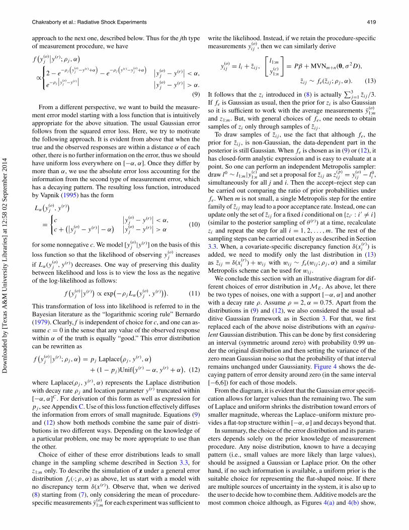
The inference proceeds as follows: we leave out about 10% ofthe data, fit the model with the remaining points as training data,and then construct point estimate and 90% predictive intervalfor each point in the test sample. This completes one trial.Randomizing selection of the test samples, we performed 50such trials, sufficient to cover all the simulator runs. Under eachmodel, we provide boxplots of average absolute bias and averagepredictive uncertainty (estimated as width of predictive interval)over all trials in Figure 5.

Although the models performed comparably for predictionbias, the average predictive uncertainty varied to a larger ex-tent from one model to another. BART generated very largepredictive intervals for the test samples. BTGP performed rela-tively better with respect to predictive uncertainty. Although thetraditional GP emulator of Kennedy and O’Hagan (2001) withglobal quadratic trend produced comparable bias estimates, us-ing a MARS mean contributed to significantly smaller uncer-tainty estimates for both (5) and (6). We specifically note that(6) fits the training dataset exactly as (4) but was still able toproduce much tighter credible intervals for the test samples. InTable 1, we summarize the bias and uncertainty results alongwith the empirical coverage rate of 90% posterior credible setconstructed for each point in the test dataset.

All the models have provided satisfactory coverage rates. Itshows that the tighter credible sets generated by MARS-basedemulators are not subject to overconfidence inaccuracy. BARTproduced the highest coverage rate but this is expected given theincreased uncertainty associated with its predictions. Based onthis statistics, we continue to work with MARS-based emulatorsin subsequent analysis.

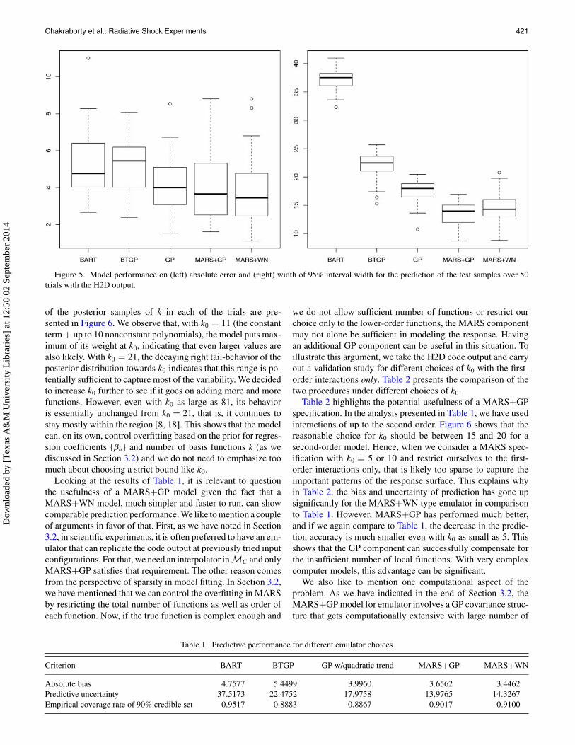
Next, we want to analyze the sensitivity of predictive perfor-mance to the choice of k0, the maximum allowed number ofbasis functions in MARS. We have mentioned this as a methodof strictly penalizing overfitting. For the H2D output, we carryout the estimation with six different values of k0 ranging from11 to 81 (including the constant function). The inverse gammaprior for σ 2

β is chosen to be proper yet diffused. The histogram

Dow

nloa

ded

by [

Tex

as A

&M

Uni

vers

ity L

ibra

ries

] at

12:

58 0

2 Se

ptem

ber

2014

Chakraborty et al.: Radiative Shock Experiments 421

Figure 5. Model performance on (left) absolute error and (right) width of 95% interval width for the prediction of the test samples over 50trials with the H2D output.

of the posterior samples of k in each of the trials are pre-sented in Figure 6. We observe that, with k0 = 11 (the constantterm + up to 10 nonconstant polynomials), the model puts max-imum of its weight at k0, indicating that even larger values arealso likely. With k0 = 21, the decaying right tail-behavior of theposterior distribution towards k0 indicates that this range is po-tentially sufficient to capture most of the variability. We decidedto increase k0 further to see if it goes on adding more and morefunctions. However, even with k0 as large as 81, its behavioris essentially unchanged from k0 = 21, that is, it continues tostay mostly within the region [8, 18]. This shows that the modelcan, on its own, control overfitting based on the prior for regres-sion coefficients {βh} and number of basis functions k (as wediscussed in Section 3.2) and we do not need to emphasize toomuch about choosing a strict bound like k0.

Looking at the results of Table 1, it is relevant to questionthe usefulness of a MARS+GP model given the fact that aMARS+WN model, much simpler and faster to run, can showcomparable prediction performance. We like to mention a coupleof arguments in favor of that. First, as we have noted in Section3.2, in scientific experiments, it is often preferred to have an em-ulator that can replicate the code output at previously tried inputconfigurations. For that, we need an interpolator inMC and onlyMARS+GP satisfies that requirement. The other reason comesfrom the perspective of sparsity in model fitting. In Section 3.2,we have mentioned that we can control the overfitting in MARSby restricting the total number of functions as well as order ofeach function. Now, if the true function is complex enough and

we do not allow sufficient number of functions or restrict ourchoice only to the lower-order functions, the MARS componentmay not alone be sufficient in modeling the response. Havingan additional GP component can be useful in this situation. Toillustrate this argument, we take the H2D code output and carryout a validation study for different choices of k0 with the first-order interactions only. Table 2 presents the comparison of thetwo procedures under different choices of k0.

Table 2 highlights the potential usefulness of a MARS+GPspecification. In the analysis presented in Table 1, we have usedinteractions of up to the second order. Figure 6 shows that thereasonable choice for k0 should be between 15 and 20 for asecond-order model. Hence, when we consider a MARS spec-ification with k0 = 5 or 10 and restrict ourselves to the first-order interactions only, that is likely too sparse to capture theimportant patterns of the response surface. This explains whyin Table 2, the bias and uncertainty of prediction has gone upsignificantly for the MARS+WN type emulator in comparisonto Table 1. However, MARS+GP has performed much better,and if we again compare to Table 1, the decrease in the predic-tion accuracy is much smaller even with k0 as small as 5. Thisshows that the GP component can successfully compensate forthe insufficient number of local functions. With very complexcomputer models, this advantage can be significant.

We also like to mention one computational aspect of theproblem. As we have indicated in the end of Section 3.2, theMARS+GP model for emulator involves a GP covariance struc-ture that gets computationally extensive with large number of

Table 1. Predictive performance for different emulator choices

Criterion BART BTGP GP w/quadratic trend MARS+GP MARS+WN

Absolute bias 4.7577 5.4499 3.9960 3.6562 3.4462Predictive uncertainty 37.5173 22.4752 17.9758 13.9765 14.3267Empirical coverage rate of 90% credible set 0.9517 0.8883 0.8867 0.9017 0.9100

Dow

nloa

ded

by [

Tex

as A

&M

Uni

vers

ity L

ibra

ries

] at

12:

58 0

2 Se

ptem

ber

2014

422 Journal of the American Statistical Association, June 2013

Table 2. Comparison of MARS+WN and MARS+GP methods with linear interactions

Method MARS+WN MARS+GP

k0 5 10 15 5 10 15

Absolute bias 3.6501 3.6098 3.4775 2.8795 2.7536 2.7512Predictive uncertainty 21.9697 21.1067 21.2541 16.4132 16.9865 17.0799Empirical coverage rate of 90% credible set 0.9250 0.9233 0.9283 0.9017 0.9033 0.8950

observations. Currently, we have only 104 outputs from the H2Dcode, but we expect to collect more and more of them over time.Thus it is relevant to discuss possible modifications we mayhave to implement in that scenario. Approximate computationmethods, as indicated in Section 3.2, can be used there. However,unlike usual GP regression for two- or three-dimensional spatialdatasets, this problem involves relatively higher-dimensional in-put space (five-dimensional input for the current experiment).We like to illustrate one specific choice that may be more conve-nient to use in this type of situations. The approach, presented inKaufman et al. (2011) in the context of a simulator related to cos-mological applications, is based on using compactly supportedcorrelation functions to ensure sparsity of GP covariance ma-trix. The range of the sparsity is controlled hierarchically andcan vary across different inputs. Since the size of the currentdataset is not large enough to efficiently represent the computa-

tional gains from this method, we decide to perform a simulationstudy. A brief description of this idea along with an evaluationof its performance with respect to predictive performance aswell as time efficiency is included in the online supplementarymaterials.

5.2 Validation With Laboratory Experiments

Now that we have evaluated different options for modeling thecode output, the next step is to validate it using outcomes fromactual laboratory experiments. In each of the eight experimentswe have results from, the shock breakout time was measuredby three different diagnostics (ASBO1, ASBO2, and SOP). Forone of those experiments, SOP measurement was not available.The ranges of measurement inaccuracy for ASBO1 (±10 ps),ASBO2 (±20 ps), and SOP (±30 ps) are converted to standard

7 8 9 10 11 8 10 12 14 16 18 20 10 15 20 25

k0 = 11 k0 = 21 k0 = 31

10 15 20 25 10 15 20 25 30 10 15 20 25 30

k0 = 41 k0 = 61 k0 = 81

Figure 6. Variation in the posterior distribution of number of local functions k under different choices of the threshold k0. The online versionof this figure is in color.

Dow

nloa

ded

by [

Tex

as A

&M

Uni

vers

ity L

ibra

ries

] at

12:

58 0

2 Se

ptem

ber

2014

Chakraborty et al.: Radiative Shock Experiments 423

Table 3. Mean absolute error and predictive uncertainty for differentemulator choices

Prediction criteria

Absolue bias UncertaintyDevicetype MARS+GP MARS+WN MARS+GP MARS+WN

ASBO1 17.6760 17.3552 72.2343 71.7667ASBO2 19.3281 18.3467 75.3237 73.4993SOP 16.2600 16.3400 81.7914 80.2587

deviations for Gaussian error distribution with the 99% proba-bility criterion used for Figure 4. Finally, in all measurements,there is a systematic timing error of ±50 ps for the laser firingmechanism. This is represented by ε0 in the model (3).

We employ the full hierarchical model in (7) using the sam-pling scheme described in Section 3.3. Here, we follow theleave-one-out validation procedure, that is, at one run, we re-move all measurements that belong to a particular experiment.Models are fitted to remaining data (simulator and experimentaloutcomes together), and similar to the above, point and intervalestimates for left-out data points are obtained from posteriordraws, which are converted to estimates of bias and uncertaintyas before. Table 3 provides the posterior mean absolute bias andpredictive uncertainty for the three models, for each of threedifferent measurement procedures.

As expected, the uncertainty estimates for ASBO1, ASBO2,and SOP measurements follow the same (increasing) order astheir individual precisions. Both of the emulators have producedcomparable bias estimates. However, using MARS+WN resultsin a slight reduction in the uncertainty estimates across all typesof measurements. We can attribute this to the additional uncer-tainty due to estimation of GP covariance parameters.

We also want to analyze, whether using an input-dependentbias function δ(x(r)) improves the prediction in MARS-basedmodels. In Table 4, we compare the average absolute error andprediction uncertainty obtained by carrying out estimation withand without the δ(·) function.

It can be seen that for neither of the emulators, adding a biasterm does not significantly alter the magnitude of predictionerror. On the other hand, the predictive uncertainty has slightlygone up in most of the cases due to the additional uncertaintyin the parameters of δ(x(r)). So, we can conclude that the H2Dalgorithm provides a satisfactory approximation of the dynamics

Table 4. Impact of bias function on prediction error and uncertainty(in parentheses)

MARS+GP MARS+WN

Device type Without δ(·) With δ(·) Without δ(·) With δ(·)ASBO1 17.6760 17.2680 17.3552 18.2971

(72.2343) (72.9123) (71.7667) (71.9894)ASBO2 19.3281 19.1712 18.3467 19.4010

(75.3237) (77.6631) (73.4993) (75.0506)SOP 16.2600 16.6120 16.3400 16.0868

(81.7914) (82.1937) (80.2587) (79.3420)

Table 5. Posterior summary for calibration parameters underMARS+WN model

Calibration parameter Be gamma Wall opacity Flux limiter

Median 1.435 1.005 0.059590% credible interval (1.402,1.483) (0.719, 1.275) (0.0504, 0.0722)

of the actual shock experiments. In the following, all subsequentanalysis are carried out without the discrepancy term δ(x(r)) inMR .

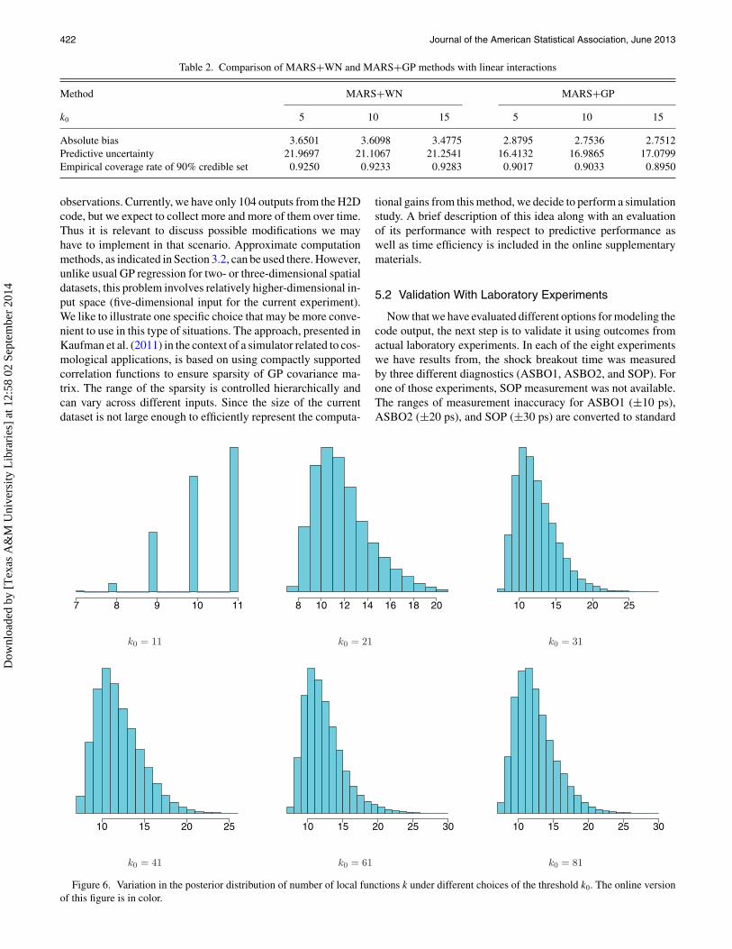
Another quantity of inferential interest is the vector of calibra-tion parameters θ (r). While designing the input configurationsfor the code, the scientists chose regularly spaced values for eachcomponent of θ (c) within a prespecified range of likely values.For each component of θ (r), we use independent uniform priorsover the set of those input configurations. Post model-fitting,we found the corresponding posterior distributions not muchsensitive to the choice of emulator model. Hence, it suffices topresent the summary statistics only for the MARS+WN modelin Table 5. Visual representation through posterior histogramsand pairwise bivariate kernel density estimates are shown inFigures 7 and 8, respectively.

The extent of nonuniformity (and peakedness) in the posteriorof each calibration parameter reflects whether the data havestrong enough evidence to identify its “correct” value in theexperiments. The posterior distribution of Be gamma, whichis seen (in Figures 7 and 8) to be concentrated only within asubregion of its prior support, looks to be the most informativeof all three quantities. However, the flux limiter has shownslightly more nonuniformity than the wall opacity. With respectto prediction, this implies that the model for shock breakouttime is more sensitive to the uncertainty in learning Be gammathan flux limiter and wall opacity.

Finally, we move to the diagnostics related to the specifi-cation of measurement error. Each of the three measurementprocedures (ASBO1, ASBO2, and SOP) is known to have adecaying error pattern (with different rates of decay), but thetiming error for the laser firing mechanism is more noninforma-tive. The laboratory does not have any further information onthe actual shock breakout time within ±50 ps of the reportedvalue. We take α = 50. For j = 1, 2, 3, ρj was determined (asabove) so that the Laplace distribution with rate ρj has 99% ofits mass inside the desired range of accuracy. Now we fit (5)and (6) with each of (9) and (12) as the choice for the measure-ment error model. All the error distributions in Figure 4 havezero mean, but quite different patterns. The range of uniformity(2α = 100 ps) is significantly large compared with the magni-tude of the response (410–504 ps). Diagnostic outputs such asmean absolute predictive bias and uncertainty are provided inTable 6 across measurement types as well as choice of errordistributions.

Notably, with both the emulators, the mean predictive abso-lute bias for all types of measurements does not vary signifi-cantly with the choice of the measurement error model. But thepredictive uncertainty is significantly affected due to the non-informativeness of the latter two specifications. The use of theLaplace–uniform mixture has resulted in the largest uncertaintyestimates, which is expected due to the flat-top nature of the

Dow

nloa

ded

by [

Tex

as A

&M

Uni

vers

ity L

ibra

ries

] at

12:

58 0

2 Se

ptem

ber

2014

424 Journal of the American Statistical Association, June 2013

Be gamma

1.40 1.45 1.50 1.55 1.60 1.65 1.70 1.75

wall opacity

0.7 0.8 0.9 1.0 1.1 1.2 1.3

flux limiter

0.050 0.055 0.060 0.065 0.070 0.075

Figure 7. Posterior density estimates for the calibration parameters in the H2D dataset. The plots correspond to the model with MARS+WNspecification. The online version of this figure is in color.

error within a ±50 ps interval around the true outcome. Bothof the emulators have shown comparable performance with re-spect to prediction bias. However, it is important to observe that,unlike the Gaussian-error-based model, MARS+GP has pro-duced slightly lower uncertainty estimates than MARS+WNwith non-Gaussian measurement error distributions across alltypes of measuring devices. Since these error distributions havemore uncertainty than an equivalent Gaussian model (as seen inFigure 4) and Table 4 shows that the simulator is a good approx-imate of the actual experiment, we can conclude that borrowingmore information from the set of simulation outputs has ac-

tually helped in marginally reducing the uncertainty withoutcompromising on the bias.

Based on the analysis in this section, MARS-based emula-tor turns out to be a flexible and efficient option for reducingthe bias and uncertainty of prediction of the shock breakouttime. It is also satisfactory to learn that the dynamics of the ac-tual experimental system can be efficiently approximated by thenumerical algorithm without the need for any discrepancy func-tion. All of the performance diagnostics presented above indi-cate that MARS+WN and MARS+GP are comparable choicesas the emulator for the H2D code. Although the former is

Dow

nloa

ded

by [

Tex

as A

&M

Uni

vers

ity L

ibra

ries

] at

12:

58 0

2 Se

ptem

ber

2014

Chakraborty et al.: Radiative Shock Experiments 425

Table 6. Comparison of different choices of the measurement error models

Measurement error model

Gaussian Laplace+uniform Laplace–uniform mixture

Criterion Device type MARS+WN MARS+GP MARS+WN MARS+GP MARS+WN MARS+GP

ASBO1 17.3552 17.6760 16.5824 15.6187 17.0972 15.9965Bias ASBO2 18.3467 19.3281 18.7290 18.5009 18.3944 14.6391

SOP 16.3400 16.2600 15.8779 17.8895 15.4721 19.1734ASBO1 71.7667 72.2343 96.8129 95.6592 104.3146 103.1104

Uncertainty ASBO2 73.4993 75.3237 98.9259 97.3865 108.0810 107.1081SOP 80.2587 81.7914 102.7600 100.3264 112.2484 111.4389

computationally much more efficient, the latter is particularlyuseful with more complex systems that would otherwise requirea large number of basis functions (as seen in Table 2). If the ob-jective of modeling is to have an emulator which is a statisticalinterpolator, that is, (i) it matches the code output at previously

used input combinations and (ii) provides an uncertainty esti-mate at a new point, MARS+GP is the only choice. It usesthe flexibility of MARS to provide uncertainty estimates forprediction at new points and, at the same time, satisfies the cri-terion of interpolation due to the GP component. Consequently,

Figure 8. Pairwise bivariate kernel density estimates for the calibration parameters in the H2D dataset. The plots correspond to the modelwith MARS+WN specification. The online version of this figure is in color.

Dow

nloa

ded

by [

Tex

as A

&M

Uni

vers

ity L

ibra

ries

] at

12:

58 0

2 Se

ptem

ber

2014

426 Journal of the American Statistical Association, June 2013

this leads to a more flexible approach to modeling nonstation-arity within a full Kennedy–O’Hagan framework relative to thecurrent literature.

6. DISCUSSION

In this article, we focused on validating the HYADES code forthe radiative shock experiments. First, we presented two differ-ent types of emulators based on adaptive splines for predictingthe shock breakout time. Their properties and relative advantageover the conventional GP emulator were discussed in Section 3,and a thorough performance analysis with the H2D output wasdone in Section 5. The data analysis shows the predictive powerof the MARS regression compared with the GP alternatives indifferent circumstances. While (5) provides a computationallyfast algorithm, the combined approach in (6) simultaneouslyuses this advantage of spline-based emulator and maintains theinterpolating behavior of MC . Another concern for using theGP emulators rises from model-fitting perspective. For the ex-perimental data, θ (r) is unknown and needs to be estimated fromthe MCMC. Although for spline-based emulators, it is involvedin the mean only, for the GP, it appears both in mean and co-variance matrix. Learning θ (r) from the not-so-well-behavedposterior distribution can be problematic. However, for specificapplications, different emulators can be preferred depending onthe practical considerations as well as the desired features of theemulator.

Another approach, similar to the MARS, is to specify f us-ing radial basis functions (Holmes and Mallick 1998). There,instead of using the tensor product of univariate local basis func-tions, weighted multivariate kernels are used around the knots. Itshould be remembered that these basis function approaches areclosely related to GP (Gibbs and Mackay 1997). Any combina-tion of such functions corresponds to the eigen decompositionof some (nonstationary) covariance kernel. Introducing a WNin the model amounts to adding a nugget with the equivalent GPprior that destroys its interpolating property.

The work in this article fits into the larger goal of the CRASHcenter to develop the predictive capability for radiating shockexperiments. In particular, the center seeks to build a frameworkthat incorporates data from shocks traveling down cylindricaltubes and then use the simulation tools to predict experimentsusing tubes of elliptical cross-sections. HYADES is a preproces-sor in the entire CRASH code in the sense that the output of theformer is the input to the latter. Thus, a hierarchical extensionof the existing model, which emulates the entire CRASH code,enables us to faithfully learn about particular aspects of the fullexperiment. Specifically, we must justify that

• our physics models are adequate,• our codes are behaving as expected, and• we understand the impact of uncertainties on code output

and prediction.

In this case, we have looked at the shock breakout time anddetermined that our physics models are capable of reproducingexperimental data after calibration; other experiment/simulationcampaigns have considered different features such as the shockposition and the total amount of shocked Xe and studied dis-crepancy between the physical model and the measurement(Holloway et al. 2011).

In the general context of the computer model validation, fur-ther improvement is possible. Any model, which combines acomputer code with a real-life experiment, consists of three ma-jor components: an emulator function for the code output, ameasurement error process for the experimental noise, and, ifnecessary, a residual function that accounts for the inadequacyof the physical model in predicting the input–output relation-ship in the real world. In this article, we have focussed onthe first two components, suggesting specifications to enhancetheir applicability in different examples. However, for the resid-ual function, we preferred to retain the zero-mean GP priorof Kennedy–O’Hagan’s (2001) setup. Small number of exper-imental outputs as well as lack of substantial prior knowledgedo not make the current dataset ideal for exploring a richer classof models for δ(·) function. However, there are examples (e.g.,experiments related to climate models) where a large number ofreal-world observations are available in addition to a complexsimulator. There, it may be of significant interest to use modelsbeyond GP, whcih allows for nonstationary patterns in the func-tion surface and incorporates any prior knowledge on the formand contributing factors of such discrepancy. Another extensionof the current model is to incorporate multivariate response (e.g.,different features of the shock such as location, speed, etc.) Si-multaneous or conditional modeling of the response can revealthe extent of association between those factors and possibly canimprove the uncertainty of the prediction by borrowing of infor-mation through the prior as well as the calibration parameters.Finally, in the goal of incorporating all possible sources of biasinside the hierarchy, a direction of future work is to consideruncertainty in measurements of x; x is treated as the fixed inputthroughout this article and thus any inference of the distributionof y is conditional on x. However, even the known inputs canhave measurement error in them. For example, laser energy isknown to exhibit a quasi-Gaussian pattern, whereas a quasi-uniform distribution is likely for Be thickness. If a stochasticmodel for x is assumed, marginal predictive uncertainty for ycan be subsequently obtained.

APPENDIX A. MARGINALIZING β AND σ2

Denote by . . . all parameters except β, σ 2. Let

Sy = yf −[

z1:m

0n

], S = Sy − Pβ.

We have,

p(yf | . . .) =∫

β

∫σ 2

p(yf |β, σ 2, . . .)p(β|σ 2)p(σ 2) dσ 2dβ,

∝ (2πσ 2

β

)−k/2∫

β

∫σ 2

(σ 2)−n+m+k

2 −aσ −1

× exp

[− 1

2σ 2

(ST D−1S + βT β/σ 2

β + 2bσ

) ]dσ 2dβ,

∝ (2πσ 2

β

)−k/2∫

β

(ST D−1S+βT β

/σ 2

β

2+bσ

)− n+m+k2 −aσ

dβ.

Now write ST D−1S + βT β/σ 2β = βT Aβ − 2βT B + C, where

A = P T D−1P + Ikσ 2β

, B = P T D−1Sy , and C = STy D−1Sy . Then

we have, ST D−1S + βT β/σ 2β + 2bσ = (β − μk)T �−1

k (β − μk) +c0k , where μk = A−1B, �k = A−1, and c0k = C − BT A−1B + 2bσ .

Dow

nloa

ded

by [

Tex

as A

&M

Uni

vers

ity L

ibra

ries

] at

12:

58 0

2 Se

ptem

ber

2014

Chakraborty et al.: Radiative Shock Experiments 427

Denote d = n + m + 2aσ . Hence,

p(yf | . . .) ∝(πσ 2

β

)−k/2c

− d+k2

0k

∫β

[1

d(β−μk)T

( c0k�k

d

)−1(β−μk) + 1

]− d+k2

dβ.

The integrand is the pdf (upto constant) for the k-variate t distributionwith mean μk , dispersion c0k�k

d, and degrees of freedom d. Hence, we

obtain the closed-form expression:

p(yf | . . .) ∝ (σ 2

β

)−k/2c

− d2

0k |�k|1/2.

APPENDIX B. RJMCMC MOVES

We first mention the prior for (k, αk) in the form of p(αk|k)p(k).As specified in (7), (k − 1) has a Poisson(λ) prior truncated at someupper bound k0. As specified, for fixed k, αk = {(nh, uh, vh, th) : h =1, 2, . . . , k}. The first term being the intercept, 2 ≤ h ≤ k correspondto the (k − 1) nonconstant functions present in the model. We requirethat these members are distinct, that is, if h �= h′, then the quadruples(nh, uh, vh, th) and (nh′ , uh′ , vh′ , th′ ) are different. If p is the total num-ber of covariates and we allow interactions up to the second order (nh =1 or 2), then number of possible choices for a nonconstant basis func-

tion is N = p + p + (p

2

) = p2+3p

2 . Allowing a particular function to bechosen repeatedly, the number of ordered choices of (k − 1) membersis Nk−1. For each of those functions, the required knots (nh many ofthem for hth basis function) can be chosen uniformly from the avail-able data points (since a change in pattern can only be detected at datapoints) and its sign can be selected in two ways—either positive ornegative with equal probability. Thus, in all, there are Nk−1(2n)

∑kh=2 nh

ordered ways of constructing αk . Now, αk is a set, so that order of thequadruples does not matter, and we are looking at only those choiceswith distinct members, so the same αk can be generated by selectingthose (k − 1) terms in any of the (k − 1)! possible permutations. Thus,prior probability of any candidate αk can be written as

p(αk|k) ∝ (k − 1)!

Nk−1(1/2n)

∑kh=2 nh .

The expression for p(αk|k) does not put zero probability on anyconfiguration whose members are not all distinct (as defined above).However, with moderately large values of N and n, the probabilityof any such duplication becomes very small. We also assume that allcovariates have n distinct values to locate a knot at; modification canbe made easily when this is not the case.

Next we specify the proposal distribution q(·, ·) for each of the threemoves as follows:

(i) First decide on the type of move to be proposed with probabil-ities bk (birth), dk (death), and ck (change), bk + dk + ck = 1.We put dk = 0, ck = 0 if k = 1, bk = 0 if k = k0.

(ii) For a birth move, choose a new basis function randomly fromthe N-set. Calculate its order nh. If this selected function doesnot agree with the existing (k − 1) nonconstant basis func-tions, then choose its knots and signs as before with probability( 1

2n)nh . Otherwise, to avoid repetition of the same polynomial

form, choose the knots and signs in (2n)nh − 1 possible ways.(iii) The death move is performed by randomly removing one of the

(k − 1) existing basis functions (excluding the constant basisfunction).

(iv) A change move consists of altering the sign and knot variablesof a randomly chosen nonconstant basis function.

From above, we have

q((k, αk) → (k′, αk′ )) =

⎧⎪⎪⎪⎪⎪⎪⎪⎨⎪⎪⎪⎪⎪⎪⎪⎩

bk

1

N

1

(2n)nk+1 − rk

k′ = k + 1,

dk

1

k − 1k′ = k − 1

ck

1

k − 1

1

(2n)nh − 1k′ = k.

In above, rk = 1 if there exists an integer h ∈ [2, k] such that nh =nk+1 and vh = vk+1, 0 otherwise. For the “change” step, h denotes theindex of basis function that has been randomly chosen for change. Theacceptance ratios for different types of move can be derived from this.

APPENDIX C. DERIVATION OF THE MIXTURE FORMFOR VAPNIK’S LOSS FUNCTION

We have the error density

f(y

(o)j

)∝⎧⎨⎩

1∣∣∣y(o)

j − y(r)∣∣∣ < α,

exp(−ρj

(∣∣∣y(o)j − y(r)

∣∣∣− α)) ∣∣∣y(o)

j − y(r)∣∣∣ > α.

For the first case above, the integral is cu = 2α. For the latter case,the integral

cl =∫

|y−y(r)|>α

exp(−ρj |y − y(r)| + ρjα

)dy

=∫

y>y(r)+α

exp(−ρj (y − y(r)) + ρjα

)dy

+∫

y<y(r)−α

exp(ρj (y − y(r)) + ρjα

)dy

= 2

ρj

Thus we have f (y(o)j ) = 1

cl+cu[g1(y(o)

j ) + g2(y(o)j )], where g1, g2 are

unnormalized Laplace(ρj , y(r), α) and Unif(y(r) − α, y(r) + α) den-

sity, respectively. After appropriate rescaling by cl and cu, we havef (y(o)

j ) = cl

cl+cuf1(y(o)

j ) + cu

cl+cuf2(y(o)

j ), where fi is the normalized ver-sion of gi , i = 1, 2. Hence, the mixture weight of first componentpj = cl

cl+cu= 1

1+ρj α.

SUPPLEMENTARY MATERIALS

The supplementary materials discuss the use of compactly sup-ported covariance function approach of Kaufman et al. (2011) insidethe MARS+GP framework; it can be useful for working with verylarge number of computer simulations.

[Received July 2011. Revised December 2012.]

REFERENCES

Arellano-Valle, R. B., Ozan, S., Bolfarine, H., and Lachos, V. H. (2005), “SkewNormal Measurement Error Models,” Journal of Multivariate Analysis, 96,265–281. [412]

Banerjee, S., Carlin, B. P., and Gelfand, A. E. (2004), Hierarchical Modelingand Analysis for Spatial Data, Boca Raton, FL: Chapman & Hall/ CRC.[415]

Banerjee, S., Gelfand, A., Finley, A., and Sang, H. (2008), “Gaussian PredictiveProcess Models for Large Spatial Data Sets,” Journal of the Royal StatisticalSociety, Series B, 70, 825–848. [415]

Barker, L. M., and Hollenbach, R. E. (1972), “Laser Interferometer for Measur-ing High Velocities of Any Reflecting Surface,” Journal of Applied Physics,43, 4669–4675. [413]

Bastos, L., and O’Hagan, A. (2009), “Diagnostics for Gaussian Process Emu-lators,” Technometrics, 51, 425–438. [412]

Dow

nloa

ded

by [

Tex

as A

&M

Uni

vers

ity L

ibra

ries

] at

12:

58 0

2 Se

ptem

ber

2014

428 Journal of the American Statistical Association, June 2013

Bayarri, M., Berger, J., Cafeo, J., Garcia-Donato, G., Liu, F., Palomo, J.,Parthasarathy, R., Paulo, R., Sacks, J., and Walsh, D. (2007), “ComputerModel Validation With Functional Output,” The Annals of Statistics, 35,1874–1906. [412]

Bayarri, M. J., Berger, J. O., Calder, E. S., Dalbey, K., Lunagomez, S., Patra, A.K., Pitman, E. B., Spiller, E. T., and Wolpert, R. L. (2009), “Using Statisticaland Computer Models to Quantify Volcanic Hazards,” Technometrics, 51,402–413. [411]

Bernardo, J. M. (1979), “Expected Information as Expected Utility,” The Annalsof Statistics, 7, 686–690. [419]

Boehly, T. R., Craxton, R. S., Hinterman, T. H., Kelly, J. H., Kessler, T. J.,Kumpan, S. A., Letzring, S. A., McCrory, R. L., Morse, S. F. B., Seka,W., Skupsky, S., Soures, J. M., Verdon, C. P. (1995), “The Upgrade to theOMEGA Laser System,” Review of Scientific Instruments, 66, 508–510.[411]

Chen, G., Gott III, J., and Ratra, B. (2003), “Non-Gaussian Error Distribution ofHubble Constant Measurements,” Publications of the Astronomical Societyof the Pacific, 115, 1269–1279. [412]

Chevalier, R. A. (1997), “Type II Supernovae SN 1987A and SN 1993J,” Science,276, 1374–1378. [411]

Chipman, H. A., George, E. I., and McCulloch, R. E. (2010), “BART: BayesianAdditive Regression Trees,” The Annals of Applied Statistics, 4, 266–298.[420]

Cressie, N., and Johannesson, G. (2008), “Fixed Rank Kriging for Very LargeSpatial Data Sets,” Journal of the Royal Statistical Society, Series B, 70,209–226. [415]

Denison, D. G. T., Holmes, C. C., Mallick, B. K., and Smith, A. F. M. (2002),Bayesian Methods for Nonlinear Classification and Regression, Chichester,UK: Wiley. [412]

Denison, D. G. T., Mallick, B. K., and Smith, A. F. M. (1998), “Bayesian Mars,”Statistics and Computing, 8, 337–346. [416]

Drake, R. P. (2006), High-Energy-Density Physics: Fundamentals, Iner-tial Fusion, and Experimental Astrophysics, Berlin/Heidelberg, Germany:Springer-Verlag. [411]

Fricker, T., Oakley, J., and Urban, N. M. (2010), “Multivariate Emulators WithNonseparable Covariance Structures,” Technical Report, MUCM TechnicalReport, University of Sheffield. [412]

Friedman, J. (1991), “Multivariate Adaptive Regression Splines,” The Annalsof Statistics, 19, 1–67. [416]

Gibbs, M., and Mackay, D. J. C. (1997), “Efficient Implementation of Gaus-sian Processes,” Technical Report, Cavendish Laboratory, Cambridge, UK.[426]

Gramacy, R. B., and Lee, H. K. H. (2008), “Bayesian Treed Gaussian Pro-cess Models With an Application to Computer Modeling,” Journal of theAmerican Statistical Association, 103, 1119–1130. [420]

Habib, S., Heitmann, K., Higdon, D., Nakhleh, C., and Williams, B. (2007),“Cosmic Calibration: Constraints From the Matter Power Spectrum and theCosmic Microwave Background,” Physical Review Letters D, 76, 083503.[411]

Higdon, D. (2002), “Space and Space-Time Modeling Using Process Convo-lutions,” in Quantitative Methods for Current Environmental Issues, eds.C. Anderson, V. Barnett, P. C. Chatwin, and A. H. El-Shaarawi, London:Springer, pp. 37–56. [415]

Higdon, D., Gattiker, J., Williams, B., and Rightley, M. (2008a), “ComputerModel Calibration Using High-Dimensional Output,” Journal of the Amer-ican Statistical Association, 103, 570–583. [412]

Higdon, D., Kennedy, M., Cavendish, J., Cafeo, J., and Ryne, R. D.(2004), “Combining Field Observations and Simulations for Calibrationand Prediction,” SIAM Journal of Scientific Computing, 26, 448–466.[412,415]

Higdon, D., Nakhleh, C., Gattiker, J., and Williams, B. (2008b), “A BayesianCalibration Approach to the Thermal Problem,” Computer Methods in Ap-plied Mechanics and Engineering, 197, 2431–2441. [411]

Holloway, J. P., Bingham, D., Chou, C., Doss, F., Drake, R. P., Fryx-ell, B., Grosskopf, M., van der Holst, B., Mallick, B. K., McClar-ren, R., Mukherjee, A., Nair, V., Powell, K. G., Ryu, D., Sokolov, I.,Toth, G., and Zhang, Z. (2011), “Predictive Modeling of a RadiativeShock System,” Reliability Engineering and System Safety, 96, 1184–1193.[426]

Holmes, C. C., and Mallick, B. K. (1998), “Bayesian Radial Basis Functions ofVariable Dimension,” Neural Computation, 10, 1217–1233. [426]

Johnson, M. E., Moore, L. M., and Ylvisaker, D. (1990), “Minimax and Max-imin Distance Designs,” Journal of Statistical Planning and Inference, 26,131–148. [414]

Kauermann, G., and Opsomer, J. D. (2011), “Data-Driven Selection ofthe Spline Dimension in Penalized Spline Regression,” Biometrika, 98,225–230. [416]

Kaufman, C. G., Bingham, D., Habib, S., Heitmann, K., and Frieman, J. A.(2011), “EFficient Emulators of Computer Experiments Using CompactlySupported Correlation Functions, With an Application to Cosmology,” TheAnnals of Applied Statistics, 5, 2470–2492. [415,422]

Kaufman, C. G., Schervish, M. J., and Nychka, D. W. (2008), “Covariance Ta-pering for Likelihood-Based Estimation in Large Spatial Data Sets,” Journalof the American Statistical Association, 103, 1545–1555. [415]

Kennedy, M., Anderson, C., O’Hagan, A., Lomas, M., Woodward, I., Gosling, J.P., and Heinemeyer, A. (2008), “Quantifying Uncertainty in the BiosphericCarbon Flux for England and Wales,” Journal of the Royal Statistical Society,Series A, 171, 109–135. [411]

Kennedy, M. C., and O’Hagan, A. (2001), “Bayesian Calibration of ComputerModels,” Journal of the Royal Statistical Society, Series B, 63, 425–464.[412,414,415,416,418,420]

Liu, F., and West, M. (2009), “A Dynamic Modelling Strategy for BayesianComputer Model Emulation,” Bayesian Analysis, 4, 393–412. [412]

Mallick, B., and Gelfand, A. E. (1995), “Bayesian Analysis of SemiparametricProportional Hazards Models,” Biometrics, 51, 843–852. [412]

Matern, B. (1960), Spatial Variation (Lecture Notes in Statistics), Berlin,Germany: Springer-Verlag. [415]

McClarren, R. G., Ryu, D., Drake, P., Grosskopf, M., Bingham, D., Chou, C.,Fryxell, B., Van der Holst, B., Holloway, J. P., Kuranz, C. C., Mallick, B.,Rutter, E., and Torralva, B. R. (2011), “A Physics Informed Emulator forLaser-Driven Radiating Shock Simulations,” Reliability Engineering andSystem Safety, 96, 1194–1207. [414]

Miller, J. E., Boehly, T. R., Melchior, A., Meyerhofer, D. D., Celliers, P. M.,Eggert, J. H., Hicks, D. G., Sorce, C. M., Oertel, J. A., and Emmel, P. M.(2007), “Streaked Optical Pyrometer System for Laser-Driven Shock-WaveExperiments on OMEGA,” Review of Scientific Instruments, 78, 034903.[413]

Neal, R. M. (1999), “Regression and Classification Using Gaussian ProcessPriors” (with discussion), in Bayesian Statistics (Vol. 6), eds. A. P. Dawid, J.M. Bernardo, J. O. Berger, and A. F. M. Smith, New York: Oxford UniversityPress, pp. 475–501. [415]

Richardson, S., and Green, P. J. (1997), “On Bayesian Analysis of MixturesWith an Unknown Number of Components,” Journal of the Royal StatisticalSociety, Series B, 59, 731–792. [417]

Rodrigues, J., and Bolfarine, H. (2007), “Bayesian Inference for an Ex-tended Simple Regression Measurement Error Model Using Skewed Priors,”Bayesian Analysis, 2, 349–364. [412]

Ruppert, D. (2002), “Selecting the Number of Knots for PenalizedSplines,” Journal of Computational and Graphical Statistics, 11, 735–757.[416]

Sacks, J., Schiller, S., and Welch, W. (1989), “Designs for Computer Experi-ments,” Technometrics, 31, 41–47. [412]

Shi, J., and Choi, T. (2011), Gaussian Process Regression Analysis for Func-tional Data, Boca Raton, FL: Chapman and Hall. [415]

Smith, M., and Kohn, R. (1998), “Nonparametric Estimation of Irregular Func-tions With Independent or Autocorrelated Errors,” in Practical Nonpara-metric and Semiparametric Bayesian Statistics, eds. D. Dey, Muller, andD. Sinha, New York: Springer-Verlag. [412]

Stefanski, L. A., and Carroll, R. J. (1987), “Conditional Scores and OptimalScores for Generalized Linear Measurement-Error Models,” Biometrika,74, 703–716. [412]

Stein, M., Chi, Z., and Welty, L. (2004), “Approximating Likelihoods for LargeSpatial Data Sets,” Journal of the Royal Statistical Society, Series B, 66,275–296. [415]

Tang, B. (1993), “Orthogonal Array-Based Latin Hypercubes,” Journal of theAmerican Statistical Association, 88, 1392–1397. [414]

Vapnik, V. N. (1995), The Nature of Statistical Learning Theory, New York:Springer-Verlag. [419]

Williams, B., Higdon, D., Gattiker, J., Moore, L., McKay, M., and Keller-McNulty, S. (2006), “Combining Experimental Data and Computer Simu-lations, With an Application to Flyer Plate Experiments,” Bayesian Analysis,1, 765–792. [411]

Dow

nloa

ded

by [

Tex

as A

&M

Uni

vers

ity L

ibra

ries

] at

12:

58 0

2 Se

ptem

ber

2014