on a kinetic equation arising in weak turbulence theory

On a kinetic equationarising in weak turbulence theory

for the nonlinear Schrodinger equation

Dissertation

zur

Erlangung des Doktorgrades (Dr. rer. nat.)

der

Mathematisch-Naturwissenschaftlichen Fakultat

der

Rheinischen Friedrich-Wilhelms-Universitat Bonn

vorgelegt von

ARTHUR HUBERTUS MARTINUS KIERKELS

aus

Heerlen

Bonn 2016

Angefertigt mit Genehmigung der Mathematisch-Naturwissenschaftlichen Fakultat derRheinischen Friedrich-Wilhelms-Universitat Bonn

1. Gutachter: Prof. Dr. Juan J. L. Velazquez2. Gutachter: Prof. Dr. Barbara Niethammer

Tag der Promotion: 12.12.2016Erscheinungsjahr: 2016

If a man is in any sense a real mathematician, then it is a hundred to one thathis mathematics will be far better than anything else he can do, and that hewould be silly if he surrendered any decent opportunity of exercising his onetalent in order to do undistinguished work in other fields.

G.H. Hardy, in [12]

v

Abstract

In this thesis we present a study of weak solutions to the following kinetic equation ofcoagulation-fragmentation type:

G(x) =1

2

∫ x

0

G(x− y)G(y)√(x− y)y

dy − G(x)√x

∫ ∞0

G(y)√y

dy

− 1

2

G(x)√x

∫ x

0

[G(y)√y

+G(x− y)√x− y

]dy +

∫ ∞0

G(x+ y)√x+ y

[G(y)√y

+G(x)√x

]dy.

(QWTE)

This quadratic equation is the leading order approximation for long times to the isotropicspace-homogeneous weak turbulence equation for the nonlinear Schrodinger equationwith defocussing cubic nonlinearity.

We first recall the weak turbulence theory for that nonlinear Schrodinger equation,and we formally derive (QWTE). We then present the general theory of weak solutionsto (QWTE), comprising among other things existence of solutions, conservation of massand energy, and convergence to equilibria. A particularly interesting feature here is theinstantaneous onset of a Dirac measure at zero for any nontrivial initial data.

The better part of this thesis is concerned with solutions to (QWTE) that exhibit self-similar behaviour. Due to the two conservation laws it is necessary to introduce a modi-fied notion of self-similarity for (QWTE). In that setting we prove existence of self-similarprofiles with finite mass, and either finite or infinite energy. We further present severalresults on the qualitative behaviour of these profiles, and we pose two conjectures thatare backed with consistency analysis and numerics.

vii

Acknowledgements

During the past years, I have had opportunities beyond imagination. It has made me theperson that I am today, and has led to the thesis you are currently reading. This wouldnot have been possible without the support of a great number of people, to whom I amtruly thankful.

Firstly, let me thank Juan J. L. Velazquez, for taking me as his student, and for providingme with a position funded by the German Science Foundation through the CRC 1060 Themathematics of emergent effects. Working with him has been a pleasure, and he will remainan example for me in years to come. From among the professorial ranks, for various otherreasons, I would further like to thank Miguel Escobedo (UPV), Rainer Kaenders, BarbaraNiethammer, and Martin Rumpf.

My experience as a PhD student would not have been the same without the (extended)research group. In particular, I thank Michael Helmers, for sharing an office, and RaphaelWinter, for making me a less bad chess player.

Also, I thank my parents. Without them, this adventure would not have been.

However, not all has been roses, and I have been extremely lucky to have had my friendsto talk to in bad times. You know who you are, and it is to you that I am most grateful.

Thuur, Bonn 2016

ix

Contents

Abstract v

Acknowledgements vii

1 Introduction 11.1 Weak turbulence theory for the nonlinear Schrodinger equation . . . . . . 2

1.1.1 The formal derivation of the weak turbulence equation . . . . . . . 21.1.2 Isotropic solutions to the weak turbulence equation . . . . . . . . . 51.1.3 Relation with the bosonic Nordheim equation . . . . . . . . . . . . 6

1.2 The quadratic weak turbulence equation . . . . . . . . . . . . . . . . . . . . 71.2.1 Connection with coagulation-fragmentation equations . . . . . . . 8

1.3 Main results, and structure of the thesis . . . . . . . . . . . . . . . . . . . . 101.4 Basic notations and definitions . . . . . . . . . . . . . . . . . . . . . . . . . 10

2 General theory 132.1 Existence of weak solutions . . . . . . . . . . . . . . . . . . . . . . . . . . . 132.2 Selected properties . . . . . . . . . . . . . . . . . . . . . . . . . . . . . . . . 172.3 The measure of the origin, and trivial solutions . . . . . . . . . . . . . . . . 19

3 Instantaneous condensation 23

4 Self-similar solutions 314.1 Existence of self-similar solutions . . . . . . . . . . . . . . . . . . . . . . . . 33

Functional analytic setting . . . . . . . . . . . . . . . . . . . . . . . . 354.1.1 Candidate self-similar profiles for ρ ∈ (1, 2) . . . . . . . . . . . . . . 364.1.2 A candidate self-similar profile in the case ρ = 2 . . . . . . . . . . . 494.1.3 Regularity of candidate profiles . . . . . . . . . . . . . . . . . . . . . 60

4.2 Properties of self-similar profiles . . . . . . . . . . . . . . . . . . . . . . . . 644.2.1 Fat tails for ρ ∈ (1, 2) . . . . . . . . . . . . . . . . . . . . . . . . . . . 654.2.2 Exponential decay for ρ = 2 . . . . . . . . . . . . . . . . . . . . . . . 674.2.3 Two conjectures, backed with consistency analysis and numerics . 70

4.3 Solutions with infinite mass . . . . . . . . . . . . . . . . . . . . . . . . . . . 74

Appendix 77A.1 Six useful lemmas . . . . . . . . . . . . . . . . . . . . . . . . . . . . . . . . . 77A.2 Postponed proofs from Chapters 1 and 4 . . . . . . . . . . . . . . . . . . . . 79

Bibliography 83

1

Chapter 1

Introduction

In the physical literature, theories of weak turbulence, or wave turbulence, are theo-ries that aim to describe the transfer of energy between different spatial frequencies inwave systems with typically weak nonlinearities. The first example can be found in [35],where it was used to describe phonon interactions in anharmonic crystals. Since then,the number of applications has expanded to also include descriptions of waves on fluidsurfaces (e.g. [14], [46], [47]), in plasmas (e.g. [44], [45]), in nonlinear optics (cf. [4]), inBose-Einstein condensates (e.g. [38,39], [40]), in the early universe (cf. [28,29]), or on elas-tic plates (cf. [3]). For a more exhausting list of examples and references, we recommendthe recent overview paper [31], or the book [30].

Any weak turbulence theory originates from a set of nonlinear wave equations, wherethe nonlinearity is small. Moreover, using the small parameter ε > 0 to quantify the non-linearity, we need to assume that setting ε = 0 yields a conservative linear system. Sup-posing further that the wave equations are solved in R× Rn, and that they are invariantunder translations in space and time, then the linearised problem can be solved usingstandard Fourier transform methods. Indeed, the space-Fourier transform u of a solutionu to this linearised problem is formally given by u(t,k) = u(0,k)e−iωt, with ω = ω(k) thereal-valued dispersion relation.

Now, the object of interest in weak turbulence theory is the density |u(t,k)|2 in wavenumber space. In the linearised case this density is constant in time due to the fact that ωis real, but for ε > 0 the evolution of |u|2 is nontrivial due to resonances between specificwave numbers k. Unfortunately, the dynamics of u also depends on its phase, so that itis in general not possible to obtain a closed equation for |u|2. However, weak turbulencetheory hypothesises that if initial data are chosen suitably, then the evolution of |u|2 canbe approximated by a kinetic equation. Solutions to that equation typically exhibit irre-versible behaviour, contrary to the underlying system of equations which is in most casestime-reversible.

Roughly speaking, and restricting to scalar-valued functions u, we suppose our initialdata to be of the form u0(k) =

√αkφk, where αk are i.i.d. random variables according to

some probability measure, and where φk are i.i.d. random phases according to the uni-form distribution on S1. We then expect to obtain a good approximation of the evolutionof |u|2 by averaging over all phases and amplitudes. For a more elaborate road map to getfrom wave equations to weak turbulence equations, we refer the reader to Part II of [30].

We should note that the precise conditions under which the aforementioned approachis valid have not been rigorously obtained. However, the derivation of kinetic equationsas above shows analogies with the formal derivation of the Boltzmann equation from thedynamics of particle systems (cf. [11], [18], [37]). In particular, the assumption of statisti-cal independence of amplitudes and phases of the initial data stands out.

2 Chapter 1. Introduction

1.1 Weak turbulence theory for NLS

In this section we summarize the theory of weak turbulence for the following nonlinearSchrodinger equation: (

i∂t + ∆x

)u = ε|u|2u, (NLS)

with u = u(t,x) : R× R3 → C, and ε > 0 small.

1.1.1 The formal derivation of the weak turbulence equation

Let us first present a formal derivation of the weak turbulence equation for (NLS), wherewe follow the reasoning in [30]. Applying the space-Fourier transform to (NLS) yields(

i∂t − |k|2)u = ε u ∗ u ∗ ˆu with ε/ε constant,

so that the function a(t,k) = u(t,k)ei|k|2t satisfies

i ˙a(k) = ε

∫∫(R3)2

a(k1)a(k2)a∗(k1 + k2 − k)ei(|k|2+|k1+k2−k|2−|k1|2−|k2|2)tdk1dk2. (1.1)

However, we note that

a(t,k)‖a(t, ·)‖2L2(R3) =

∫∫(R3)2

a(t,ki)a(t,kj)a∗(t,ki + kj − k)δ0(ki − k)dkidkj ,

so that the contribution to the right hand side of (1.1) that comes from the integral over thesubmanifolds k1 = k and k2 = k is purely real, and thus only accounts for a changein the phase of a. Noting also that ‖a(t, ·)‖L2(R3) = ‖u(t, ·)‖L2(R3) = ‖u(0, ·)‖L2(R3), wherethe second identity is due to Plancherel’s theorem, and the conservation laws of solutionsto (NLS) (cf. [41]), we may then introduce the function

a(t,k) = u(t,k) expi|k|2t+ 2iε‖u(0, ·)‖2L2(R3)t

,

which satisfies

ia(k) = ε

∫∫(R3)2

a(k1)a(k2)a∗(k1 + k2 − k)Ek,k1+k2−kk1,k2

(t)dk1dk2, (1.2)

with the shorthand

Er3,r4r1,r2 (τ) =

0 if r1 = r3 & r2 = r4 or r1 = r4 & r2 = r3,

ei(|r3|2+|r4|2−|r1|2−|r2|2)τ else.

(1.3)

Next, we write a as the formal series in ε around an initial field b with random phase andamplitude, i.e. we set

a(t,k) = b(k) + εa1(t,k) + ε2a2(t,k) + · · · , (1.4)

with b(k) = |b(k)|φk, where |b(k)|2 are i.i.d. according to some probability measure, andwhere all φk are independent and uniformly distributed over S1. Introducing further thebrackets 〈·〉 to denote averaging over the probability distributions of |b(k)|2 and φk, then

1.1. Weak turbulence theory for the nonlinear Schrodinger equation 3

using (1.4) we get that⟨|a(t,k)|2

⟩−⟨|b(k)|2

⟩= ε 2<

⟨b∗(k)a1(t,k)

⟩+ ε2

(⟨|a1(t,k)|2

⟩+ 2<

⟨b∗(k)a2(t,k)

⟩)+ · · · . (1.5)

Thus, in order to obtain an equation for 〈|a(t,k)|2〉 to leading order in ε, we are requiredto express a1 and a2 in terms of b, which is easily done using (1.4) in (1.2):

a1(t,k) = −i∫∫

(R3)2b(k1)b(k2)b∗(k1 + k2 − k)

∫ t

0Ek,k1+k2−k

k1,k2(s)ds dk1dk2, (1.6)

a2(t,k) = −i∫ t

0

∫∫(R3)2

b(k1)b(k2)a∗1(s,k1 + k2 − k)Ek,k1+k2−kk1,k2

(s)dk1dk2 ds

− 2i

∫ t

0

∫∫(R3)2

b(k1)a1(s,k2)b∗(k1 + k2 − k)Ek,k1+k2−kk1,k2

(s)dk1dk2 ds, (1.7)

where (1.6) is to be substituted into (1.7). Writing now 〈·〉φ for the average over only thephases, we observe that⟨

φr1φr2φ∗r3φ∗r4

⟩φ

= δ0(r3 − r1)δ0(r4 − r2) + δ0(r4 − r1)δ0(r3 − r2)

− δ0(r2 − r1)δ0(r3 − r2)δ0(r4 − r3),

which, using (1.3), implies that⟨b(r1)b(r2)b∗(r3)b∗(r4)

⟩φ× Er3,r4

r1,r2 ≡ 0. (1.8)

In particular we thus have< 〈b∗(k)a1(t,k)〉φ = 0, whereby the first term on the right handside of (1.5) vanishes. In order to compute 〈|a1(t,k)|2〉φ we next find⟨

φk1φk2φ∗k1+k2−kφ

∗k3φ∗k4

φk3+k4−k⟩φ

∣∣∣ki=k

=⟨φk1φk2φ

∗kφ∗k1+k2−k

⟩φ

for i ∈ 3, 4, (1.9)

and a similar expression for i ∈ 1, 2, whereby, with again (1.8), we conclude that

⟨|a1(t,k)|2

⟩φ

= 2

∫∫(R3)2

|b(k1)|2|b(k2)|2|b(k1 + k2 − k)|2∣∣∣∣∣∫ t

0Ek,k1+k2−k

k1,k2(s)ds

∣∣∣∣∣2

dk1dk2.

For 〈b∗(k)a2(t,k)〉φ we now write b∗(k)a2(t,k) = I1(t,k) + 2I2(t,k), where I1 and I2 arethe products of b∗(k) and, respectively, the first and second integrals on the right handside of (1.7). Similar to (1.9), we here get

⟨φ∗kφk1φk2φ

∗k3φ∗k4

φk3+k4−(k1+k2−k)

⟩φ

∣∣∣ki=k

=⟨φ∗k3

φ∗k4φkjφk3+k4−kj

⟩φ

for i, j ∈ 1, 2 and i 6= j,

and ⟨φ∗kφk1φk3φk4φ

∗k3+k4−k2

φ∗k1+k2−k⟩φ

∣∣∣k1=k

=⟨φk3φk4φ

∗k2φ∗k3+k4−k2

⟩φ,

which, together with (1.8), leads to the expressions

〈I1(t,k)〉φ = 2|b(k)|2∫∫

(R3)2|b(k1)|2|b(k2)|2

∫ t

0

∫ s

0Ek,k1+k2−k

k1,k2(s− σ)dσds dk1dk2,


and

〈I2(t,k)〉φ = −1

2× 2|b(k)|2

∫∫(R3)2

(|b(k1)|2 + |b(k2)|2

)|b(k1 + k2 − k)|2

×∫ t

0

∫ s

0Ek,k1+k2−k

k1,k2(s− σ)dσds dk1dk2.

Observing lastly for Ω ∈ R that

1

t

∣∣∣∣∣∫ t

0eiΩsds

∣∣∣∣∣2

=1

t× 2<

(∫ t

0

∫ s

0eiΩ(s−σ)dσds

)= 1

t

(2Ω sin

(Ωt2

))2=: ðt(Ω),

we thus find that (1.5) to leading order in ε equals⟨|a(t,k)|2

⟩−⟨|b(k)|2

⟩= ε2t

(η(t,k) +

⟨|b(k)|2

⟩γ(t,k)

), (1.10)

with

η(t,k) = 2

∫∫∫(R3)3

⟨|b(k1)|2

⟩⟨|b(k2)|2

⟩⟨|b(k4)|2

⟩× ðt(|k|2 + |k4|2 − |k1|2 − |k2|2)δ0(k + k4 − k1 − k2)dk1dk2dk4,

and

γ(t,k) = 2

∫∫∫(R3)3

(⟨|b(k1)|2

⟩⟨|b(k2)|2

⟩−(⟨|b(k1)|2

⟩+⟨|b(k2)|2

⟩)⟨|b(k4)|2

⟩)× ðt(|k|2 + |k4|2 − |k1|2 − |k2|2)δ0(k + k4 − k1 − k2)dk1dk2dk4.

However, the characteristic evolution time of 〈|a(t,k)|2〉 is now of order 1ε2

, so that forε2t 1, replacing the left hand side of (1.10) by t ∂t〈|a(t,k)|2〉, we get

∂t⟨|a(t,k)|2

⟩= ε2

(η(t,k) +

⟨|b(k)|2

⟩γ(t,k)

). (1.11)

Moreover, as we are interested in the limit ε→ 0, it is reasonable to suppose that (1.11) isvalid for all t ≥ 0. Observing lastly that ðt → 2πδ0 as t→∞, we finally obtain for t ε2

that the function n(k) = n(t,k) = limε→0〈|a( tε2,k)|2〉 = 〈|b(k)|2〉 satisfies

n(k) = 4π

∫∫∫(R3)3

(n(k1)n(k2)

(n(k) + n(k4)

)−(n(k1) + n(k2)

)n(k)n(k4)

)× δ0(|k|2 + |k4|2 − |k1|2 − |k2|2)δ0(k + k4 − k1 − k2)dk1dk2dk4, (WTE)

the space-homogeneous weak turbulence equation associated to the defocussing nonlin-ear Schrodinger equation (NLS).

We would like to emphasize again that the above derivation is only formal. Despitethe fact that (WTE) has been frequently studied, both in its own right (cf. [4], [30], [48]),and in the context of Bose-Einstein condensation (cf. [15], [17], [36], [38, 39], [40]), its rig-orous derivation is still a largely open problem. However, for first rigorous results in thecase of the discrete nonlinear Schrodinger equation, see [25] and [26, 27].

1.1. Weak turbulence theory for the nonlinear Schrodinger equation 5

1.1.2 Isotropic solutions to the weak turbulence equation

The paper [9] presents a number of results on isotropic solutions to (WTE), i.e. solutionsof the form n(k) = f(|k|2). Now, using this as an ansatz in (WTE), switching to sphericalcoordinates with k = |k|, and using the integral expression of δ0, we obtain

f(k2) = 4π

∫∫∫[0,∞)3

W(f(k2

1)f(k22)(f(k2) + f(k2

4))−(f(k2

1) + f(k22))f(k2)f(k2

4))

× δ0(k2 + k24 − k2

1 − k22)dk1dk2dk4,

with

W = W (k1, k2, k, k4) = k21k

22k

24 ×

∫∫∫(S2)3

[1

(2π)3

∫R3

eis·(k+k4−k1−k2)ds

]dΩ1dΩ2dΩ4

= 8k1k2k4 ×4π

k

∫ ∞0

sin(k1s) sin(k2s) sin(ks) sin(k4s)ds

s2,

where the integral on the right hand side evaluates to π4 mink1, k2, k, k4 (cf. [39], [7], or

Lemma 6 in [Kie16]). Making then the change of variables to ω = k2, and integrating outthe remaining Dirac delta, we find that f must satisfy

f(ω) = 4π3

∫∫[0,∞)2

K√ω

(f(ω1)f(ω2)

(f(ω) + f(ω1 + ω2 − ω)

)−(f(ω1) + f(ω2)

)f(ω)f(ω1 + ω2 − ω)

)dω1dω2, (1.12)

with K = K(ω1, ω2, ω) = min√ω1,√ω2,√ω,√

(ω1 + ω2 − ω)+. However, we will seethat it is actually more convenient to study g(ω) = (2π)3/2√ωf(ω), which satisfies

g(ω) =1

2

∫∫[0,∞)2

K

[g(ω1)√ω1

g(ω2)√ω2

(g(ω)√ω

+g(ω1 + ω2 − ω)√ω1 + ω2 − ω

)

−(g(ω1)√ω1

+g(ω2)√ω2

)g(ω)√ω

g(ω1 + ω2 − ω)√ω1 + ω2 − ω

]dω1dω2, (CWTE)

withK as before. Indeed, integrating (CWTE) against a function ϕ, using the abbreviatednotations fi = g(ωi)/

√ωi andϕi = ϕ(ωi) for i ∈ 1, 2, 3, 4, and exploiting the symmetries

of the equation, we find that∫[0,∞)

ϕ(ω)g(ω)dω =1

2

∫··∫

[0,∞)4δ0(ω3 + ω4 − ω1 − ω2)K(ω1, ω2, ω3)

×[f1f2

(f3 + f4

)−(f1 + f2

)f3f4

]ϕ3 dω1··dω4

=1

4

∫··∫

[0,∞)4δ0K

[f1f2

(f3 + f4

)−(f1 + f2

)f3f4

](ϕ3 + ϕ4

)dω1··dω4

=1

4

∫··∫

[0,∞)4δ0K

[f1f2

(f3 + f4

)](ϕ3 + ϕ4 − ϕ1 − ϕ2

)dω1··dω4, (1.13)

where, since we only integrate over the submanifold ω3 +ω4 = ω1 +ω2, the right handside vanishes for ϕ ≡ 1 and ϕ(ω) = ω. The evolution of (CWTE) thus formally conservesboth the integral and the first moment, which we prefer over the conservation of themoments 1

2 and 32 by the evolution of (1.12). Moreover, integrating (1.13) with respect to


the time variable, we obtain∫[0,∞)

ϕ(ω)g(t, ω)dω −∫

[0,∞)ϕ(ω)g(0, ω)dω =

∫ t

0C4[g(s, ·)](ϕ)ds (1.14)

with

C4[g](ϕ) =1

2

∫∫∫[0,∞)3

K(ω1, ω2, ω3)√ω1ω2ω3

(ϕ(ω3) + ϕ(ω1 + ω2 − ω3)− ϕ(ω1)− ϕ(ω2)

)×g(ω1)g(ω2)g(ω3) dω1dω2dω3. (1.15)

which is well-defined for suitable g and ϕ (cf. Lemma A.1). It is therefore natural to use(1.14) in order to define the notion of a weak solution to (CWTE), as was done in [9].

The weak formulation allows us to assign a particle interpretation to (CWTE). Indeed,if we suppose g(t, ω) to be a distribution of particles of sizes ω ≥ 0 at time t, then the inter-action mechanism is as follows: Two particles of sizes ω1, ω2 ≥ 0 interact to produce twoparticles of sizes ω3, ω4 ≥ 0 with ω3 +ω4 = ω1 +ω2, where the incidence rate of interactionis proportional to

K(ω1, ω2, ω3)√ω1ω2ω3

× g(t, ω1)g(t, ω2)g(t, ω3).

In particular, an interaction can only take place if either of the two resulting particle sizesis already present in the distribution. However, if no particles of size 0 are present, thenthe interaction ω1, ω2 → ω1 + ω2, 0will not take place, since K(ω1, ω2, ω1 + ω2) = 0.

ω1

ω2ω3

ω4

FIGURE 1.1: Collision mechanism in the particle interpretation of (CWTE).Two particles of sizes ω1, ω2 ≥ 0 interact to produce two particles of sizesω3, ω4 ≥ 0 with ω3 + ω4 = ω1 + ω2, where the rate of interaction dependson the amount of particles of sizes ω1, ω2, and ω3, that are already presentin the distribution.

Besides global existence of weak solutions to (CWTE), it was shown in [9] that the in-tegral and the first moment of a weak solution are invariant. Noting that these conservedquantities correspond to the ones of the linear Schrodinger, being the norms in L2(R3)and H1(R3), we will further refer to the integral of a solution as its mass, and to the firstmoment as its energy. However, it was also shown that all solutions with mass m ≥ 0converge in the sense of measures to a Dirac delta with massm at ω ≥ 0, where ω denotesthe infimum of all sizes of particles that can be obtained by the collision mechanism. Sincefor most solutions there holds ω = 0, and since the energy of a Dirac delta at 0 is zero, thisindicates that there has to be some transfer of energy towards infinity. This is the topic ofthis thesis.

1.1.3 Relation with the bosonic Nordheim equation

Though weak turbulence theory for (NLS) is interesting in its own right, the weak turbu-lence equation is strongly related to the bosonic Nordheim equation, which was derivedby Nordheim as the quantum analogue to the Boltzmann equation (cf. [34]). Its isotropic

1.2. The quadratic weak turbulence equation 7

form is given by

f(ω) =

∫∫[0,∞)2

K√ω

(f(ω1)f(ω2)

(f(ω) + f(ω1 + ω2 − ω) + 1

)−(f(ω1) + f(ω2) + 1

)f(ω)f(ω1 + ω2 − ω)

)dω1dω2, (BNE)

which differs only from (CWTE) in the occurrence of the regular quadratic Boltzmannterms in the integral on the right hand side. The connection between these equations hasbeen pointed out by several authors (cf. e.g. [4], [17], [30]), and it is thought that the cubicterms should be the dominant ones in certain limits. Indeed, many of the results that wereobtained in [7, 8] for (BNE) are similar to the ones in [9] for (CWTE), and it is because ofthis that we refer to the onset of a Dirac delta in (CWTE) as the formation of a condensate.For further results on the quantum Boltzmann equation, we refer the reader to [20–23].

1.2 The quadratic weak turbulence equation

In order to better understand the transfer of energy towards infinity, we suppose that thelong time behaviour of weak solutions to (CWTE) can be approximated by the perturba-tion of a Dirac mass. To that end we consider weak solutions g to (CWTE) of the form g =δ0 +G, where G is a nonnegative measure-valued function with mass 0 < ε 1. In thissection we determine the evolution equation for G in the limit ε → 0, which is the equa-tion of interest in this thesis.

Now, we want to use the ansatz g(t, ·) = δ0 +G(t, ·) in (1.14), to which end we first setg = δ0 +G in (1.15). This gives us

C4[δ0 +G](ϕ) = C4[G](ϕ) + C1233 [G](ϕ) + C231

3 [G](ϕ) + C3123 [G](ϕ)

+ C1232 [G](ϕ) + C231

2 [G](ϕ) + C3122 [G](ϕ) + C4[δ0](ϕ), (1.16)

with

Cijk3 [G](ϕ) =1

2

∫∫∫[0,∞)3

K(ω1, ω2, ω3)√ω1ω2ω3

(ϕ(ω3) + ϕ(ω1 + ω2 − ω3)− ϕ(ω1)− ϕ(ω2)

)×G(ωi)G(ωj)δ0(ωk) dω1dω2dω3,

and

Cijk2 [G](ϕ) =1

2

∫∫∫[0,∞)3

K(ω1, ω2, ω3)√ω1ω2ω3

(ϕ(ω3) + ϕ(ω1 + ω2 − ω3)− ϕ(ω1)− ϕ(ω2)

)×G(ωi)δ0(ωj)δ0(ωk) dω1dω2dω3,

where, by symmetries in the integrands, we immediately note that C2313 [G] ≡ C312

3 [G] andC123

2 [G] ≡ C2312 [G]. We then interpret the last seven terms on the right hand side of (1.16)

as particle interactions where one or more of the particles ω1, ω2, ω3 ≥ 0 have size 0. If allare zero particles, i.e. if ω1 = ω2 = ω3 = 0, then ω4 = 0, which suggests C4[δ0] ≡ 0. Further,ω1 = ω2 = 0 implies ω3 = ω4 = 0, and if ω1 = ω3 = 0 or ω2 = ω3 = 0, then we respectivelyget ω4 = ω2 or ω4 = ω1, which is an indication that C123

2 [G] ≡ C2312 [G] ≡ C312

2 [G] ≡ 0. Thiscan now be formalized using Lemma A.1, whereby the integrand in the right hand sideof (1.15) vanishes on the axes ω1 = ω2 = 0, ω1 = ω3 = 0, and ω2 = ω3 = 0, and we


find that∫[0,∞)

ϕ(ω)G(t, ω)dω −∫

[0,∞)ϕ(ω)G(0, ω)dω

=

∫ t

0

[C4[G(s, ·)](ϕ) + C123

3 [G(s, ·)](ϕ) + 2 C2313 [G(s, ·)](ϕ)

]ds. (1.17)

Integrating out the Dirac deltas, we now get that

C1233 [G](ϕ) =

1

2

∫∫[0,∞)2

G(ω1)G(ω2)√ω1ω2

(ϕ(0) + ϕ(ω1 + ω2)− ϕ(ω1)− ϕ(ω2)

)dω1dω2,

and

C2313 [G](ϕ) =

1

2

∫∫ω2≥ω3≥0

G(ω2)G(ω3)√ω2ω3

(ϕ(ω3) + ϕ(ω2 − ω3)− ϕ(0)− ϕ(ω2)

)dω2dω3,

which are well-defined for suitable G and ϕ [cf. (A.2) and (A.3)]. We then combine theseterms to obtain

C3[G](ϕ) := C1233 [G](ϕ) + 2 C231

3 [G](ϕ)

=1

2

∫∫R2+

G(x)G(y)√xy

(ϕ(x+ y) + ϕ(|x− y|)− 2ϕ(maxx, y)

)dxdy, (1.18)

which in view of Lemma 1.6 is well-defined for suitableG and ϕ. Normalizing lastlyG toa probability measure, we find from (1.17) and (1.18) that G(t, ·) = limε→0

1εG( tε , ·) must

satisfy ∫[0,∞)

ϕ(ω)G(t, ω)dω −∫

[0,∞)ϕ(ω)G(0, ω)dω =

∫ t

0C3[G(s, ·)](ϕ)ds (1.19)

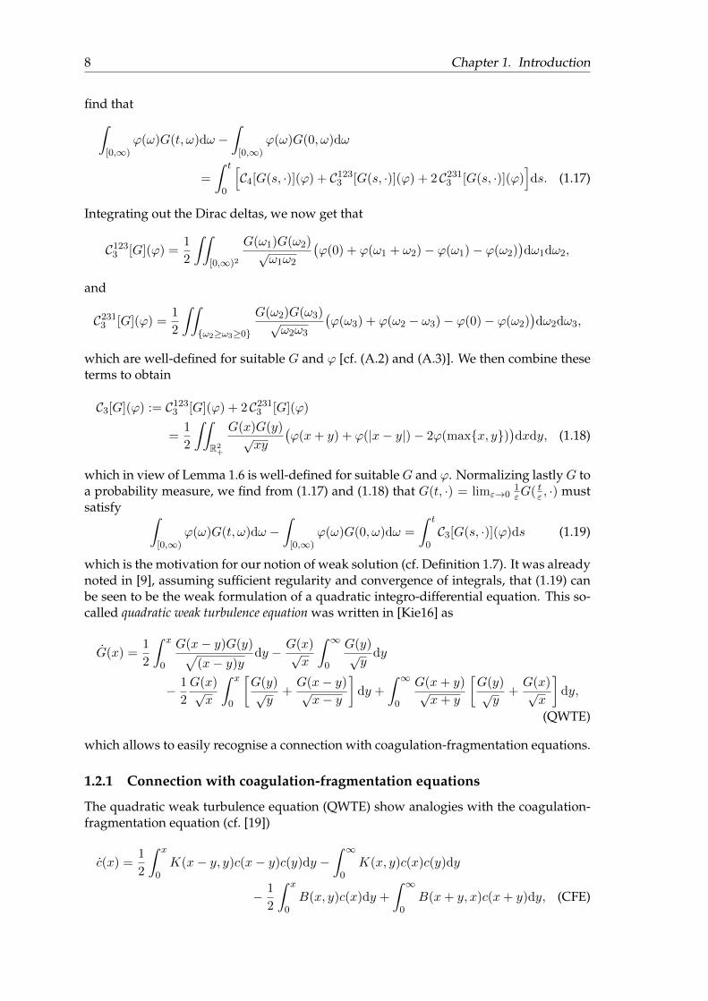
which is the motivation for our notion of weak solution (cf. Definition 1.7). It was alreadynoted in [9], assuming sufficient regularity and convergence of integrals, that (1.19) canbe seen to be the weak formulation of a quadratic integro-differential equation. This so-called quadratic weak turbulence equation was written in [Kie16] as

G(x) =1

2

∫ x

0

G(x− y)G(y)√(x− y)y

dy − G(x)√x

∫ ∞0

G(y)√y

dy

− 1

2

G(x)√x

∫ x

0

[G(y)√y

+G(x− y)√x− y

]dy +

∫ ∞0

G(x+ y)√x+ y

[G(y)√y

+G(x)√x

]dy,

(QWTE)

which allows to easily recognise a connection with coagulation-fragmentation equations.

1.2.1 Connection with coagulation-fragmentation equations

The quadratic weak turbulence equation (QWTE) show analogies with the coagulation-fragmentation equation (cf. [19])

c(x) =1

2

∫ x

0K(x− y, y)c(x− y)c(y)dy −

∫ ∞0

K(x, y)c(x)c(y)dy

− 1

2

∫ x

0B(x, y)c(x)dy +

∫ ∞0

B(x+ y, x)c(x+ y)dy, (CFE)

1.2. The quadratic weak turbulence equation 9

y

x

K(x, y)

B(x+ y, y)

x+ y

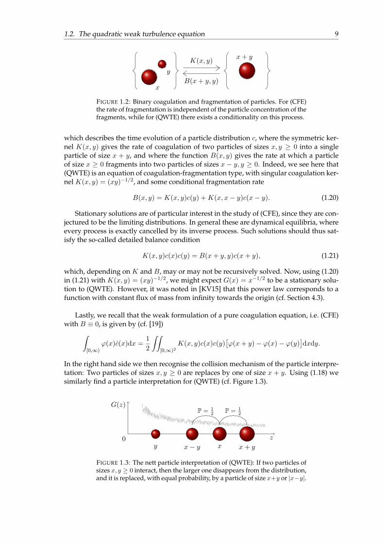
FIGURE 1.2: Binary coagulation and fragmentation of particles. For (CFE)the rate of fragmentation is independent of the particle concentration of thefragments, while for (QWTE) there exists a conditionality on this process.

which describes the time evolution of a particle distribution c, where the symmetric ker-nel K(x, y) gives the rate of coagulation of two particles of sizes x, y ≥ 0 into a singleparticle of size x + y, and where the function B(x, y) gives the rate at which a particleof size x ≥ 0 fragments into two particles of sizes x − y, y ≥ 0. Indeed, we see here that(QWTE) is an equation of coagulation-fragmentation type, with singular coagulation ker-nel K(x, y) = (xy)−1/2, and some conditional fragmentation rate

B(x, y) = K(x, y)c(y) +K(x, x− y)c(x− y). (1.20)

Stationary solutions are of particular interest in the study of (CFE), since they are con-jectured to be the limiting distributions. In general these are dynamical equilibria, whereevery process is exactly cancelled by its inverse process. Such solutions should thus sat-isfy the so-called detailed balance condition

K(x, y)c(x)c(y) = B(x+ y, y)c(x+ y), (1.21)

which, depending on K and B, may or may not be recursively solved. Now, using (1.20)in (1.21) with K(x, y) = (xy)−1/2, we might expect G(x) = x−1/2 to be a stationary solu-tion to (QWTE). However, it was noted in [KV15] that this power law corresponds to afunction with constant flux of mass from infinity towards the origin (cf. Section 4.3).

Lastly, we recall that the weak formulation of a pure coagulation equation, i.e. (CFE)with B ≡ 0, is given by (cf. [19])∫

[0,∞)ϕ(x)c(x)dx =

1

2

∫∫[0,∞)2

K(x, y)c(x)c(y)[ϕ(x+ y)− ϕ(x)− ϕ(y)

]dxdy.

In the right hand side we then recognise the collision mechanism of the particle interpre-tation: Two particles of sizes x, y ≥ 0 are replaces by one of size x + y. Using (1.18) wesimilarly find a particle interpretation for (QWTE) (cf. Figure 1.3).

0 z

G(z)P = 1

2 P = 12

y xx− y x+ y

FIGURE 1.3: The nett particle interpretation of (QWTE): If two particles ofsizes x, y ≥ 0 interact, then the larger one disappears from the distribution,and it is replaced, with equal probability, by a particle of size x+y or |x−y|.


1.3 Main results, and structure of the thesis

Most of the results that are presented in this thesis have already appeared in the papers[KV15,KV16], and in the preprint [Kie16]. The arguments in these publications have beenmerged, in particular on the level of notation, and we have tried to simplify our proofs asmuch as possible.

In Chapter 2 we present the general theory of weak solutions to (QWTE), comprising aproof of existence, the conservation laws of (QWTE), and some monotonicity results. Thisis essentially the first part of [KV15]. That paper also discusses the phenomenon of instan-taneous condensation, i.e. the immediate onset of a Dirac mass at zero for all initial data,and we present a simplified proof here in Chapter 3. As a corollary we then get our firstmain result, which we may state as

Theorem. A weak solution to (QWTE) has either got a strictly growing condensateat the origin, or it is time-independent.

A modified notion of self-similar solution to (QWTE) with finite mass was introducedin the final part of [KV15] for finite energy, and then extended in [KV16] to also includesolutions with infinite energy. In Section 4.1 we present severely modified proofs of theexistence results in those papers (cf. Remark 4.5), which form our second main result:

Theorem. There are weak solutions to (QWTE) that transfer their (possibly infinite)energy towards infinity in a self-similar manner.

The rigorous results on qualitative behaviour of self-similar profiles, obtained in [KV16],as well as two conjectures from [Kie16], can now be found in Section 4.2.

1.4 Basic notations and definitions

In the final section of this introduction we present notations and definitions that will beused throughout the thesis. The functional analytic setting in which we prove existenceof self-similar profiles will be introduced later, on page 35.

We start with some spaces of functions.

Definition 1.1. Given an interval I ⊂ [−∞,∞], we denote by C(I) the space of real-val-ued functions that are continuous at every point x ∈ I , byCc(I) the subspace of functionsf ∈ C(I) for which suppf ⊂ I , and by C0(I) the closure of Cc(I) in L∞(R).

Given further k ∈ N and α ∈ (0, 1], let Ck(I) be the subspace of functions f ∈ C(I)that are k times differentiable on I with f (`) ∈ C(I) for all ` ∈ 1, . . . , k, let Ckc (I) be thesubspace of functions f ∈ Ck(I) for which suppf ⊂ I , let Ck0 (I) be the closure of Ckc (I) inW k,∞(R), let C0,α(I) be the subspace of functions f ∈ C(I) that are α-Holder continuouson all compact sets K ⊂ I , and let Ck,α(I) be the subspace of functions f ∈ Ck(I) forwhich f (k) ∈ C0,α(I).

Lastly, set C∞(I) =⋂k∈NC

k(I), C∞c (I) =⋂k∈NC

kc (I), and C∞0 (I) =

⋂k∈NC

k0 (I).

It should be noted that the previous definition is the usual one for I ⊂ R. The notion ofcontinuity at infinity for a function f ∈ C(I), where ∞ ∈ I , equates to existence in Rof the limit limx→∞ f(x).

We then define spaces of Radon measures by duality.

Definition 1.2. Given an interval I ⊂ [0,∞], we define the space M(I) of Radon mea-sures on I to be the space of bounded linear functionals on C0(I), i.e.M(I) = (C0(I))′.The subspace of nonnegative Radon measures is denoted by M+(I), and the space of

1.4. Basic notations and definitions 11

nonnegative Radon measures with unit measure, i.e. the space of probability measures,is denoted by P(I).

Furthermore, we write M+(0,∞) for the subset of measures µ ∈ M+([0,∞]) forwhich µ(∞) = 0.

We will always write µ(x)dx to denote integration with respect to a measure µ, even ifthe measure is not absolutely continuous with respect to the Lebesgue measure. Also, wewrite ‖µ‖ =

∫I |µ(x)|dx for any µ ∈M(I).

The spaces of measures are endowed with their natural coarsest topologies.

Definition 1.3. Given an interval I ⊂ [0,∞], we endow the spaceM(I), and its subspacesM+(I) and P(I), with the weak-∗ topology, which is the coarsest topology such that forevery ϕ ∈ C0(I) the mapping µ 7→

∫I ϕ(x)µ(x)dx is continuous.

Since further Cc([0,∞)) ⊂ C([0,∞]) = Cc([0,∞]), henceM+([0,∞]) ⊂ M+([0,∞)),we may endow M+(0,∞) with the weak-∗ topology ofM+([0,∞)).

We note here that, since (C0(I), ‖ · ‖L∞(I)) is a separable Banach space, we can uniquelycharacterize convergence with respect to the weak-∗ topology in the following manner:A sequence µn ⊂ M(I) converges with respect to the weak-∗ topology to µ ∈ M(I),for short µn ∗ µ inM(I), if and only if

∫Iϕ(x)µn(x)dx→

∫Iϕ(x)µ(x)dx for all ϕ ∈ C0(I).

Definition 1.4. We define our frequently used notations.

• Given a function f ∈ C(R), we will denote by ∆2yf(x) the second order central dif-

ference of size y ∈ R at x ∈ R, i.e. we define

∆2yf(x) = f(x+ y) + f(x− y)− 2f(x).

• For x, y ∈ R we use the notations x ∨ y = maxx, y and x ∧ y = minx, y, and foru ∈ R we write (u)+ = max0, u.

? Given a function ϕ ∈ C([0,∞]), then the first two items of this definition allow usto write ϕ(x+ y) + ϕ(|x− y|)− 2ϕ(maxx, y) = ∆2

x∧yϕ(x ∨ y) for x, y ≥ 0.

• We write R+ for the set of strictly positive real numbers, i.e. R+ = (0,∞).

• Given functions f, g ∈ C(R+), then if there holds limz→$f(z)g(z) = 1 with $ ∈ 0,∞,

then we write f(z) ∼ g(z) as z → $.

Lastly, we introduce the notion of weak solution to (QWTE). We will need two furtherlemmas, whose elementary proofs can be found in the appendix.

Lemma 1.5. Given a function G ∈ C([0,∞) : M+(0,∞)), then for every T ≥ 0 there holds

supt∈[0,T ] ‖G(t, ·)‖ <∞.

Lemma 1.6. Given a function ϕ ∈ Cc([0,∞)) ∩W 1,∞(0,∞) for which ϕ′ is continuous in aneighbourhood of 0, let F ∈ C(R2

+) be the symmetric function that for x > y > 0 satisfies

F (x, y) =1√xy

(ϕ(x+ y) + ϕ(x− y)− 2ϕ(x)

),

i.e. F (x, y) = 1√xy∆2

x∧yϕ(x ∨ y). Then F extends by zero to the closure of R2+, i.e. F ∈ C0(R2

+).


These lemmas allow us to pose the following

Definition 1.7. We call G a weak solution to (QWTE) if (i) G ∈ C([0,∞) : M+(0,∞)),i.e. the mapping t 7→ G(t, ·) is continuous from [0,∞) into M+(0,∞), endowed with theweak-∗ topology on (C0([0,∞)))′; and (ii) for all t ≥ 0 and ϕ ∈ C([0,∞) : C1

c ([0,∞))) ∩C1([0,∞) : Cc([0,∞))) there holds∫

[0,∞)ϕ(t, x)G(t, x)dx−

∫[0,∞)

ϕ(0, x)G(0, x)dx−∫ t

0

∫[0,∞)

ϕs(s, x)G(s, x)dx ds

=

∫ t

0

1

2

∫∫R2+

G(s, x)G(s, y)√xy

∆2x∧y[ϕ(s, ·)](x ∨ y)dxdy ds (QWTE)w

with ∆2x∧y[ϕ(s, ·)](x ∨ y) = ϕ(s, x+ y) + ϕ(s, |x− y|)− 2ϕ(s, x ∨ y) (cf. Definition 1.4).

13

Chapter 2

General theory

In this chapter we present the general theory of weak solutions to (QWTE). Global exis-tence is shown in Section 2.1, and in Section 2.2 we prove several basic properties of solu-tions, such as uniform tightness, a scaling result, and their conservation laws. In the finalSection 2.3 we introduce the notion of a stationary trivial solution. We further show thatthe weak-∗ limit of any weak solution to (QWTE) is trivial in that sense.

2.1 Existence of weak solutions

We will prove the following

Theorem 2.1. Given G0 ∈ M+(0,∞), there exists at least one weak solution G to (QWTE) inthe sense of Definition 1.7 that satisfies G(0, ·) ≡ G0 on [0,∞).

The way to prove Theorem 2.1 is quite standard: We replace the kernel (xy)−1/2 by a netof bounded approximations, prove existence of solutions to these approximate problemsby means of a fixed-point argument, and finally show that in the limit we obtain a weaksolution to (QWTE). Our approximating kernels will be ((x + ε)(y + ε))−1/2 with ε > 0,but in view of the product decomposition of this function we prove Lemma 2.2 below,which is slightly more general.

Lemma 2.2. Given a nonnegative function k ∈ C0([0,∞)), then for anyG0 ∈M+([0,∞]) thereexists at least oneG ∈ C([0,∞) :M+([0,∞])) that for all t ≥ 0 and ϕ ∈ C1([0,∞) : C([0,∞]))satisfies∫

[0,∞]ϕ(t, x)G(t, x)dx−

∫[0,∞]

ϕ(0, x)G0(x)dx−∫ t

0

∫[0,∞]


=

∫ t

0

1

2

∫∫[0,∞)2

G(s, x)G(s, y) k(x)k(y)∆2x∧y[ϕ(s, ·)](x ∨ y) dxdy ds. (2.1)

In particular, there holds ‖G(t, ·)‖ = ‖G0‖ for all t ≥ 0.

Proof. If either k ≡ 0 orG0 ≡ 0, then clearlyG(t, ·) ≡ G0 satisfies (2.1) for all t ≥ 0 and ϕ ∈C1([0,∞) : C([0,∞])). We thus suppose that ‖k‖L∞(0,∞) =: κ > 0 and ‖G0‖ =: M > 0,and we fix T = (8κ2M)−1 > 0.

For ε > 0 arbitrarily fixed, we now set φε(x) = 1εφ(xε ) with φ(x) = (1− |x|)+. We then

first show that there exists at least on Gε ∈ C([0, T ] : M+([0,∞])) that for all t ∈ [0, T ]and ϕ ∈ C([0,∞]) satisfies∫

[0,∞]ϕ(x)Gε(t, x)dx =

∫[0,∞]

ϕ(x)e−∫ t0 Aε[Gε(s,·)](x)dsG0(x)dx

+

∫ t

0

∫[0,∞]

ϕ(x)e−∫ tσ Aε[Gε(s,·)](x)dsBε[Gε(σ, ·)](x)dx dσ, (2.2)

14 Chapter 2. General theory

where Aε :M+([0,∞])→ C0([0,∞)) is given by

Aε[G](x) = 2k(x)

∫[0,∞)

∫ x

0φε(y − z)k(z)dz G(y)dy ≥ 0,

and where Bε :M+([0,∞])→M+([0,∞]) is such that for any ϕ ∈ C([0,∞]) there holds∫[0,∞]

ϕ(x)Bε[G](x)dx

=

∫∫[0,∞)2

G(x)G(y) k(x)

∫ x

0φε(y − z)k(z)(ϕ(x+ z) + ϕ(x− z))dz dxdy.

Note that both mappings Aε and Bε are continuous due to the additional regularization,achieved by convolving with φε. Therefore, the right hand side of (2.2) is continuous asa function of t on [0, T ] for all Gε ∈ C([0, T ] : M+([0,∞])) and ϕ ∈ C([0,∞]), whencewe can define a mapping Tε from C([0, T ] : M+([0,∞])) into itself such that for all G ∈C([0, T ] :M+([0,∞])), t ∈ [0, T ], and ϕ ∈ C([0,∞]) there holds∫

[0,∞]ϕ(x)Tε[G](t, x)dx =

∫[0,∞]

ϕ(x)e−∫ t0 Aε[G(s,·)](x)dsG0(x)dx

+

∫ t

0

∫[0,∞]

ϕ(x)e−∫ tσ Aε[G(s,·)](x)dsBε[G(σ, ·)](x)dx dσ. (2.3)

Using then first ϕ ≡ 1 in (2.3), we find for all t ∈ [0, T ] that

‖Tε[G](t, ·)‖ ≤ ‖G0‖+ 2κ2

∫ t

0‖G(σ, ·)‖2dσ ≤ ‖G0‖+ 2κ2

(supt∈[0,T ]

‖G(t, ·)‖

)2

T,

and it follows with our choice of T > 0 that Tε maps X = G ∈ C([0, T ] : M+([0,∞])) :supt∈[0,T ] ‖G(t, ·)‖ ≤ 2M into itself. For G ∈ X , 0 ≤ t1 ≤ t2 ≤ T , and ϕ ∈ C([0,∞]), wefurther find that∫

[0,∞]ϕ(x)Tε[G](t2, x)dx−

∫[0,∞]

ϕ(x)Tε[G](t1, x)dx

=

∫[0,∞]

(e−

∫ t2t1Aε[G(s,·)](x)ds − 1

)ϕ(x)Tε[G](t1, x)dx

+

∫ t2

t1

∫[0,∞]

ϕ(x)e−∫ t2σ Aε[G(s,·)](x)dsBε[G(σ, ·)](x)dx dσ,

where the absolute value of the right hand side can be estimated by∫[0,∞]

(∫ t2

t1

Aε[G(s, ·)](x)ds

)‖ϕ‖L∞(0,∞)Tε[G](t1, x)dx

+

∫ t2

t1

∫[0,∞]

‖ϕ‖L∞(0,∞)Bε[G(σ, ·)](x)dx dσ

≤ ‖ϕ‖L∞(0,∞)

(∫ t2

t1

2κ2‖G(s, ·)‖ds ‖Tε[G](t1, ·)‖+

∫ t2

t1

2κ2‖G(σ, ·)‖2dσ

).

2.1. Existence of weak solutions 15

For all G ∈ X , t1, t2 ∈ [0, T ], and ϕ ∈ C([0,∞]), there thus holds∣∣∣∣∣∫

[0,∞]ϕ(x)Tε[G](t2, x)dx−

∫[0,∞]

ϕ(x)Tε[G](t1, x)dx

∣∣∣∣∣ ≤ 16κ2M2‖ϕ‖L∞(0,∞)|t2 − t1|,

hence Tε[X ] ⊂ X is precompact, by Arzela-Ascoli (cf. Chapter 7 in [16]). By Schauder’sfixed-point theorem there then indeed exists at least on Gε ∈ C([0, T ] :M+([0,∞])) suchthat Tε[Gε] ≡ Gε, which indeed satisfies (2.2) for all t ∈ [0, T ] and ϕ ∈ C([0,∞]). We nextcheck that for t ∈ [0, T ] and ϕ ∈ C1([0, T ] : C([0,∞])) it further satisfies∫

[0,∞]ϕ(t, x)Gε(t, x)dx−

∫[0,∞]

ϕ(0, x)G0(x)dx−∫ t

0

∫[0,∞]

ϕs(s, x)Gε(s, x)dx ds

=

∫ t

0

∫∫[0,∞)2

Gε(s, x)Gε(s, y) k(x)

∫ x

0φε(y − z)k(z)∆2

z[ϕ(s, ·)](x)dz dxdy ds. (2.4)

Indeed, given t ∈ [0, T ] and ϕ ∈ C1([0, T ] : C([0,∞])), it follows from (2.2) that[∫[0,∞]

ϕ(t, x)Gε(t, x)dx

]t

=

∫[0,∞]

ϕt(t, x)Gε(t, x)dx

−∫

[0,∞)ϕ(t, x)Aε[Gε(t, ·)](x)Gε(t, x)dx+

∫[0,∞]

ϕ(t, x)Bε[Gε(t, ·)](x)dx,

which when integrated yields (2.4).We now consider a collection G = Gεε>0 ⊂ X , where for every ε > 0 we require

that Gε ≡ Tε[Gε]. Since (2.3) is independent of ε, it follows by again Arzela-Ascoli thatthere exist a subsequence ε→ 0, and G ∈ X , such that Gε(t, ·) ∗ G(t, ·), uniformly for allt ∈ [0, T ]. For all t ∈ [0, T ] and ϕ ∈ C1([0, T ] : C([0,∞])) the left hand side of (2.4) thentrivially converges to the left hand side of (2.1). Now, using Fubini, we rewrite the righthand side of (2.4) as∫ t

0

1

2

∫∫[0,∞)2

Gε(s, x)Gε(s, y)

[∫ x

0φε(y − z)k(x)k(z)∆2

z[ϕ(s, ·)](x)dz

+

∫ y

0φε(x− z)k(y)k(z)∆2

z[ϕ(s, ·)](y)dz

]dxdy ds, (2.5)

where the term between square brackets converges uniformly for all x, y ≥ 0 and t ∈[0, T ] to

k(x)k(y)∆2x∧y[ϕ(s, ·)](x ∨ y),

(cf. Lemma A.5). Recalling then for all ε > 0 that supt∈[0,T ] ‖Gε(t, ·)‖ ≤ 2‖G0‖, it followsthat the limit of (2.5) as ε→ 0 coincides with

limε→0

∫ t

0

1

2

∫∫[0,∞)2

Gε(s, x)Gε(s, y) k(x)k(y)∆2x∧y[ϕ(s, ·)](x ∨ y) dxdy ds,

which, using the decay at infinity of k, can be checked to be equal to the right hand sideof (2.1).

For any G0 ∈M+([0,∞]) we thus have some G ∈ C([0, T ] :M+([0,∞])) that satisfies(2.1) for all t ∈ [0, T ] and ϕ ∈ C1([0, T ] : C([0,∞])), and in particular ‖G(t, ·)‖ = ‖G0‖ forall t ∈ [0, T ]. Iterating this construction lastly yields the desired function G ∈ C([0,∞) :M+([0,∞])) that satisfies (2.1) for all t ≥ 0 and ϕ ∈ C1([0,∞) : C([0,∞])).


We are now set to prove existence of weak solutions to (QWTE).

Proof of Theorem 2.1. Given G0 ∈ M+(0,∞) ⊂ M+([0,∞]), then, following Lemma 2.2,for any ε > 0 there exists at least one Gε ∈ C([0,∞) : M+([0,∞])) that for all t ≥ 0 andϕ ∈ C1([0,∞) : C([0,∞])) satisfies∫

[0,∞]ϕ(t, x)Gε(t, x)dx−

∫[0,∞]

ϕ(0, x)G0(x)dx−∫ t

0

∫[0,∞]

ϕs(s, x)Gε(s, x)dx ds

=

∫ t

0

1

2

∫∫[0,∞)2

Gε(s, x)Gε(s, y)∆2x∧y[ϕ(s, ·)](x ∨ y)√

(x+ ε)(y + ε)dxdy ds. (2.6)

We first check that Gε(t, ·) ∈M+(0,∞) for all ε > 0 and t ≥ 0, which we do by showingthat the collection G = Gε(t, ·)ε>0,t≥0 is uniformly tight. We thereto fix ε > 0 and t ≥ 0,and for R > 0 we set ϕR(x) = (1 − x

R)+, which is convex and nonincreasing, and whichin particular satisfies 1[0,R) ≥ ϕR ≥ ϕR(r)1[0,r] for any r ≥ 0. Using then ϕ ≡ ϕR as atime-independent test function in (2.6), the right hand side is nonnegative by convexityof ϕR (cf. Lemma A.2), hence there holds∫

[0,∞]ϕR(x)Gε(t, x)dx ≥

∫[0,∞]

ϕR(x)G0(x)dx,

and in particular∫[0,R)

Gε(t, x)dx ≥(

1− 1√R

)∫[0,√R]G0(x)dx for all R ≥ 1.

Combining this with the fact that ‖Gε(t, ·)‖ = ‖G0‖ for all t ≥ 0 and ε > 0 (cf. Lemma2.2), it thus follows for R ≥ 1 that∫

[R,∞]Gε(t, x)dx ≤

∫[0,∞)

G0(x)dx−(

1− 1√R

)∫[0,√R]G0(x)dx

where the right hand side vanishes as R→∞, independently of ε > 0 and t ≥ 0, and weconclude that G is a uniformly tight subset of M+(0,∞).

For ϕ ∈ C1([0,∞]) we next find that∣∣∣∣∣ ∆2x∧yϕ(x ∨ y)√

(x+ ε)(y + ε)

∣∣∣∣∣ ≤ 2‖ϕ‖W 1,∞(0,∞) for all x, y ≥ 0 and ε > 0,

(cf. Lemma A.3), so using ϕ ∈ C1([0,∞]) as a time-independent test function in (2.6), wefind for t1, t2 ≥ 0 that∣∣∣∣∣

∫[0,∞]

ϕ(x)Gε(t2, x)dx−∫

[0,∞]ϕ(x)Gε(t1, x)dx

∣∣∣∣∣ ≤ ‖G0‖2‖ϕ′‖L∞(0,∞) |t2 − t1|.

Now, since C1([0,∞]) is dense in C([0,∞]), it follows that for any ϕ ∈ C([0,∞]) thecollection of mappings

t 7→∫

[0,∞]ϕ(x)Gε(t, x)dx

ε>0

is equicontinuous. By Arzela-Ascoli we then obtain existence of a subsequence ε → 0,and a function G ∈ C([0,∞) :M+([0,∞])), such that Gε(t, ·) ∗ G(t, ·), locally uniformly

2.2. Selected properties 17

for all t ∈ [0,∞). Moreover, it can be checked that there hold G(t, ·)t≥0 ⊂ M+(0,∞),and G(0, ·) ≡ G0 on [0,∞).

We complete the proof by checking thatG is a weak solution to (QWTE). It is immedi-ate that the left hand side of (2.6) converges to the left hand side of (QWTE)w for all t ≥ 0and ϕ ∈ C1([0,∞) : C([0,∞])). For any time-independent test function ϕ ∈ C1([0,∞]),we further notice that the fraction in the right hand side of (2.6) converges uniformly forall x, y ≥ 0 to the continuous function in C0(R2

+) that for x, y > 0 is given by

∆2x∧yϕ(x ∨ y)√xy

,

(cf. Lemma A.6). Combining then the decay at infinity of this limit function with uniformtightness of G, we find for any t ≥ 0 and ϕ ∈ C([0,∞) : C1([0,∞])) that the right handside of (2.6) converges to the right hand side of (QWTE)w, hence G satisfies (QWTE)w forall t ≥ 0 and ϕ ∈ C([0,∞) : C1([0,∞])) ∩ C1([0,∞) : C([0,∞])). Thus, restricting to testfunctions that in space are compactly supported in [0,∞), and recalling that the weak-∗topology onM+([0,∞)) is weaker than the one onM+([0,∞]), we conclude that G is aweak solution to (QWTE) in the sense of Definition 1.7.

2.2 Selected properties

In this section we prove some elementary properties of weak solutions to (QWTE). Thefollowing monotonicity lemma will be useful throughout.

Lemma 2.3. Let G be weak solution to (QWTE), and let ϕ ∈ C0([0,∞)) be convex [concave].Then the mapping

t 7→ H[ϕ](t) :=

∫[0,∞)

ϕ(x)G(t, x)dx (2.7)

is continuous and nondecreasing [nonincreasing] on [0,∞).

Proof. We may restrict ourselves to proving monotonicity, since continuity follows imme-diately from the use of the weak-∗ topology. Moreover, since H[ϕ] ≡ −H[−ϕ], it sufficesto consider the case where ϕ is convex. In that case, there is a sequence ϕn ⊂ C1

c ([0,∞))of convex functions such that ϕ ≡ supn ϕn. By monotone convergence there then holdsH[ϕ] ≡ supnH[ϕn], hence it suffices to check monotonicity of H[ϕn] for all n. We theretouse any ϕn as a time-independent test function in (QWTE)w, which for t ≥ 0 yields

H[ϕn](t) = H[ϕn](0) +

∫ t

0

1

2

∫∫R2+

G(s, x)G(s, y)√xy

∆2x∧yϕn(x ∨ y)dxdy ds. (2.8)

Since the integrand in the second term on the right hand side of (2.8) is nonnegative byconvexity of ϕn (cf. Lemma A.2), it thus follows that H[ϕn] is indeed nondecreasing as afunction of t on [0,∞).

In the proof of Theorem 2.1 we saw that Gε(t, ·)ε>0,t≥0 was a uniformly tight subsetof M+(0,∞). The result and its proof carry over naturally to weak solutions to (QWTE):

Proposition 2.4. Let G be a weak solution to (QWTE), and let η,R > 0 be arbitrary. Then thereholds ∫

[0,Rη

]G(t, x)dx ≥ (1− η)

∫[0,R]

G(0, x)dx for all t ≥ 0.


Proof. Using ϕ(x) = (1 − η xR)+ in Lemma 2.3, the function H[ϕ] is nondecreasing. Fur-thermore, there holds 1[0,R

η] ≥ ϕ ≥ (1− η)+1[0,R], so for all t ≥ 0 we have∫

[0,Rη

]G(t, x)dx ≥ H[ϕ](t) ≥ H[ϕ](0) ≥ (1− η)+

∫[0,R]

G(0, x)dx,

and the claim follows easily.

Our notion of weak solution to (QWTE) requires only that (QWTE)w is satisfied fortest functions with compact support in [0,∞). However, one can check that weak solu-tions satisfy (QWTE)w for more test functions.

Lemma 2.5. Let G be a weak solution to (QWTE). Then G also satisfies (QWTE)w for all t ≥ 0and ϕ ∈ C([0,∞) : C1([0,∞])) ∩ C1([0,∞) : C([0,∞])).

Proof. For all n ∈ N, let ζn(x) =∫∞x φ(x − n)dx with φ(x) = (1 − |x|)+. Given now

ϕ ∈ C([0,∞) : C1([0,∞])) ∩ C1([0,∞) : C([0,∞])), we set ϕn(t, x) = ϕ(t, x)ζn(x), whichfor any n ∈ N is an admissible test function in (QWTE)w, and we note that ϕn(t, ·) and∂tϕn(t, ·) converge to ϕ(t, ·) and ϕt(t, ·) as n → ∞, pointwise on [0,∞) and uniformlyfor all t ≥ 0. Recalling then Lemma 1.5, for all t ≥ 0 it is immediate by dominatedconvergence that∫

[0,∞)ϕ(t, x)G(t, x)dx−

∫[0,∞)

ϕ(0, x)G(0, x)dx−∫ t

0

∫[0,∞)


= limn→∞

∫ t

0

1

2

∫∫R2+

G(s, x)G(s, y)√xy

∆2x∧y[ϕn(s, ·)](x ∨ y)dxdy ds, (2.9)

and using also Lemma A.6, convergence of the right hand side of (2.9) follows as well.

The previous result in particular allows to use ϕ ≡ 1 as a test function in order to getconservation of mass. We can further use that result to find that initially finite energiesare conserved.

Proposition 2.6. Given a weak solution G to (QWTE), then ‖G(t, ·)‖ = ‖G(0, ·)‖ for all t ≥ 0.Moreover, if G(0, ·) has finite first moment, then there holds∫

[0,∞)xG(t, x)dx =

∫[0,∞)

xG(0, x)dx for all t ≥ 0. (2.10)

Proof. Using ϕ ≡ 1 as a time-independent test function in (QWTE)w, which is possiblefollowing Lemma 2.5, it immediately follows that ‖G(t, ·)‖ = ‖G(0, ·)‖ for all t ≥ 0.

For ε > 0, let now H[ϕε] be given by (2.7) with ϕε(x) = x1+εx , and note that H[ϕε]

is nonincreasing (cf. Lemma 2.3). Moreover, invoking again Lemma 2.5 to use ϕε as atime-independent test function in (QWTE)w, for t ≥ 0 there holds

0 ≤ H[ϕε](0)−H[ϕε](t) =

∫ t

0

1

2

∫∫R2+

G(s, x)G(s, y)√xy

∣∣∆2x∧yϕε(x ∨ y)

∣∣ dxdy ds. (2.11)

For x, y ≥ 0 we further explicitly compute that

∣∣∆2x∧yϕε(x ∨ y)

∣∣ =2ε(x ∧ y)2

(1 + ε(x+ y))(1 + ε(x ∨ y))(1 + ε|x− y|)≤ 2ε(x ∧ y)ϕε(y),

2.3. The measure of the origin, and trivial solutions 19

and using this estimate we can bound the right hand side of (2.11) from above by

ε

∫ t

0

∫∫R2+

G(s, x)G(s, y)ϕε(y)dxdy ds ≤ ‖G(0, ·)‖t εH[ϕε](0). (2.12)

Now, if the first moment of G(0, ·) is bounded, then by monotone convergence it is equalto the limit limε→0H[ϕε](0). For any fixed t ≥ 0, the right hand side of (2.12) then thusvanishes as ε→ 0, hence so does the right hand side of (2.11), and there holds

limε→0

∫[0,∞)

x1+εxG(t, x)dx =

∫[0,∞)

xG(0, x)dx. (2.13)

We then conclude the claim since the left hand sides of (2.13) and (2.10) coincide by againmonotone convergence.

We end this section with a straightforward scaling result.

Lemma 2.7. Let G be a weak solution G to (QWTE), and let κ1, κ2 > 0 be arbitrary. Then alsoG ∈ C([0,∞) : M (0,∞)), defined to be such that∫

[0,∞)ϕ(x)G(t, x)dx =

∫[0,∞)

ϕ( xκ2 )κ1G(κ1κ2t, x)dx for t ≥ 0 and ϕ ∈ C([0,∞)),

is a weak solution to (QWTE), and there holds ‖G(t, ·)‖ = κ1‖G(0, ·)‖ for all t ≥ 0.

Proof. Immediate from elementary manipulations.

2.3 The measure of the origin, and trivial solutions

We now take a closer look at the measure of the origin of a weak solutionG to (QWTE). Inthe particle interpretation (cf. Figure 1.3) we see that only the larger one of two interactingparticles is taken from the distribution. A particle of size 0 can thus only disappear due tointeraction with another zero-particle. However, the particle is then replaced by a particleof size 0, which doesn’t contribute to a nett change in the distribution. (Alternatively, inthe particle interpretation of (CWTE), this corresponds to an interaction of three particlesω1, ω2, ω3 ≥ 0 where two of them are zero-particles, which indeed does not affect the totaldistribution.) We therefore expect that the number of particles of size 0 cannot decrease,which can be formalized as follows.

Proposition 2.8. Given a weak solution G to (QWTE), then the mapping

t 7→ m(t) :=

∫0

G(t, x)dx

is right-continuous and nondecreasing on [0,∞).

Proof. DefiningH[ϕn] by (2.7) withϕn(x) = (1−nx)+ and n ∈ N, we havem ≡ infnH[ϕn].Monotonicity of m is then immediate from monotonicity of H[ϕn] (cf. Lemma 2.3), andsince for t ≥ 0 we further observe that

m(t) ≤ lim sups→t+

m(s) ≤ infn∈N

(lims→t

H[ϕn](s))

= infn∈N

H[ϕn](t) = m(t),

right-continuity also follows.


As an immediate consequence of the monotonicity of the mass of the origin, we obtainthe following uniqueness result.

Corollary 2.9. Givenm ≥ 0, then the weak solutionG to (QWTE) withG(0, ·) ≡ mδ0 is uniqueand time-independent, i.e. G(t, ·) ≡ mδ0 for all t ≥ 0.

Proof. Given a weak solution G to (QWTE) that satisfies G(0, ·) ≡ mδ0, which exists byTheorem 2.1, then for all t ≥ 0 there holds

0 ≤∫

(0,∞)G(t, x)dx = m−

∫0

G(t, x)dx, (2.14)

(cf. Propositions 2.6). Moreover, since the right hand side of (2.14) is monotonically de-creasing as a function of t (cf. Proposition 2.8), it follows that it is bounded from aboveby 0, and we conclude the claim.

This now motivates the introduction of the notion of a trivial solution.

Definition 2.10. We say that G is a trivial solution to (QWTE) if it is a weak solution in thesense of Definition 1.7 that satisfies supp(G(0, ·)) ⊂ 0. A weak solution to (QWTE) thatis not trivial will be called nontrivial.

The argumentation preceding Proposition 2.8 seems to suggest that zero-particles aresomehow unconnected to the other particles in the distribution. Indeed, we find that wemay add and subtract zero-particles to move between weak solutions to (QWTE).

Lemma 2.11. Let G be a weak solution to (QWTE), and let m ∈ R be arbitrary. Then G, givenby

G(t, ·) ≡ mδ0 +G(t, ·) on [0,∞) for t ≥ 0,

satisfies (QWTE)w for all t ≥ 0 and ϕ ∈ C([0,∞) : C1c ([0,∞))) ∩ C1([0,∞) : Cc([0,∞))).

Moreover, if m+∫0G(0, x)dx ≥ 0, then G is actually a weak solution to (QWTE).

Proof. Since the product measure δ0 × δ0 is supported outside the domain of integrationon the right hand side of (QWTE)w, the claim holds if G is the zero solution G ≡ 0. If Gis an arbitrary weak solution to (QWTE), then G is a linear combination of functions thatsatisfy (QWTE)w for all t ≥ 0 and ϕ ∈ C([0,∞) : C1

c ([0,∞))) ∩ C1([0,∞) : Cc([0,∞))).It thus suffices to check that the cross terms vanish, which follows from the observationthat the product measures δ0 × G(t, ·) with t ≥ 0 are also supported outside the domainof integration on the right hand side of (QWTE)w. Lastly, due to monotonicity of themeasure of the origin (cf. Proposition 2.8) the initial estimate is sufficient to guaranteethat G(t, ·) ≥ 0 on [0,∞) for all t ≥ 0, which makes G a weak solution.

Lastly, it is natural to expect solutions to a kinetic equation to converge in some senseto their equilibria. Despite not having proven uniqueness of the equilibrium solutions to(QWTE) (yet, but see Corollary 3.2), we can show weak-∗ convergence to trivial solutions.

Proposition 2.12. Given a weak solution G to (QWTE), then G(t, ·) ∗ ‖G(0, ·)‖δ0 as t→∞.

Proof. Since the claim is immediate for trivial solutions, we suppose without loss of gen-erality thatG is nontrivial. Setting then ϕ(x) = e−x in Lemma 2.3, we obtain a continuousand nondecreasing function H that for all t ≥ 0 satisfies

H(t) = H(0) +

∫ t

0

1

2

∫∫R2+

G(s, x)G(s, y)√xy

e−(x∨y)(e

12

(x∧y) − e−12

(x∧y))2

dxdy ds, (2.15)

2.3. The measure of the origin, and trivial solutions 21

and noticing further that

H(t) =

∫[0,∞)

e−xG(t, x)dx ≤∫

[0,∞)G(t, x)dx =: M for all t ≥ 0,

(cf. Proposition 2.6), it follows that limt→∞H(t) = supt≥0H(t) =: L ≤ M exists. We willnext check that L = M , to which end we conversely suppose that L < M . Defining thena = log(1 + M−L

2M+L) > 0, we observe for all s ≥ 0 that∫[0,a]

G(s, x)dx ≤ ea∫

[0,∞)e−xG(s, x)dx ≤

(1 +

M − L2M + L

)L < L+ 1

3(M − L),

hence there holds∫(a,∞)

G(s, x)dx = M −∫

[0,a]G(s, x)dx > 2

3(M − L) for all s ≥ 0. (2.16)

We can then further choose some R > a such that∫[0,R]

G(0, x)dx ≥M − 16(M − L) =

5M + L

6,

and setting η = 1− 4M+2L5M+L and b = R

η , we use Proposition 2.4 to obtain that∫[0,b]

G(s, x)dx ≥ 2M + L

3= M − 1

3(M − L) for all s ≥ 0. (2.17)

Combining (2.16) and (2.17), it now follows that∫(a,b]

G(s, x)dx =

∫[0,b]

G(s, x)dx+

∫(a,∞)

G(s, x)dx−M > 13(M −L) for all s ≥ 0, (2.18)

and using (2.18) in (2.15) we find for all t ≥ 0 that

H(t) ≥∫ t

0

1

2

∫∫(a,b]2

G(s, x)G(s, y)√xy

e−(x∨y)(e

12

(x∧y) − e−12

(x∧y))2

dxdy ds

≥ 2be−b sinh2(a2 )

∫ t

0

(∫(a,b]

G(s, x)dx

)2

ds > 19C(a, b)(M − L)2 t.

Since this contradicts the boundedness of H , we thus have L = M , and we find that anyweak-∗ limit of G is supported at the origin. Arguing lastly by compactness for existenceof such limits, the claim follows.

23

Chapter 3

Instantaneous condensation

We have seen that the measure of the origin of a weak solution to (QWTE) is nondecreas-ing (cf. Proposition 2.8). In this chapter we will prove that this measure is actually strictlyincreasing as long as the solution does not coincide with a trivial one, i.e. we prove

Theorem 3.1. Given a weak solution G to (QWTE) in the sense of Definition 1.7, then for everyt ≥ 0 for which

∫(0,∞)G(t, x)dx > 0, there holds∫

0G(t, x)dx >

∫0

G(t, x)dx for all t > t.

As a consequence of this result, we obtain the characterization of time-independent weaksolutions to (QWTE) as the unique trivial ones.

Corollary 3.2. A weak solution to (QWTE) is time-independent if and only if it is trivial in thesense of Definition 2.10.

Proof. From Corollary 2.9 we know that trivial solutions are time-independent. Suppos-ing conversely that G is a nontrivial weak solution to (QWTE), then in particular thereholds

∫(0,∞)G(0, x)dx > 0, and G cannot be time-independent by Theorem 3.1.

Let us briefly outline the proof of Theorem 3.1. We note first that (QWTE) is invariantunder time-translations, so that we may restrict ourselves to t = 0. Moreover, in view ofLemma 2.11 it is sufficient to show that, given a nontrivial weak solution G to (QWTE) thatsatisfies

∫0G(0, x)dx = 0, then there holds∫

0G(t, x)dx > 0 for all t > 0. (3.1)

Indeed, given any nontrivial weak solution G to (QWTE), by that lemma we can defineanother weak solution G by

G(t, ·) ≡ G(t, ·)−

(∫0

G(0, x)dx

)δ0 on [0,∞) for t ≥ 0,

which has initially zero mass at the origin. The instantaneous onset of a Dirac delta at theorigin for G then implies the strict monotonicity of the measure of the origin of G, by thefact that ∫

0G(t, x)dx > 0 ⇔

∫0

G(t, x)dx >

∫0

G(0, x)dx.

We now conversely suppose that (3.1) does not hold, which by monotonicity of the mea-sure of the origin (cf. Proposition 2.8) implies the existence of some finite T > 0 for which∫

0G(s, x)dx = 0 for all s ∈ [0, T ],

24 Chapter 3. Instantaneous condensation

and for which thus∫ 23T

13T

∫[0,r]

G(s, x)dx ds =

∫ 23T

13T

∫(0,r]

G(s, x)dx ds for all r ≥ 0. (3.2)

In the following we will prove lower and upper bounds on the left and right hand sidesof (3.2) respectively, from which a contradiction will follow. The proofs of these boundsrely heavily on the following two lemmas, as well as on Proposition 2.4.

Two lemmas

Lemma 3.3. Let G be a weak solution to (QWTE), and for n ∈ N let (z0, . . . , zn) ∈ Rn+1+ be

such that zi − zi−1 ∈ (0, 12z0] for all i ∈ 1, . . . , n. Then for all t ≥ 0 there holds

∫[0,z0]

G(t, x)dx ≥ 1

4

∫ t

0

n∑i=1

1

zi

(∫(zi−1,zi]

G(s, x)dx

)2ds.

Proof. Let ϕ ∈ C1c ([0,∞)) be convex, and such that ϕ(x) ≤ 1

z0(z0−x)+ for all x ≥ 0. Using

then ϕ as a time-independent test function in (QWTE)w, we easily find for t ≥ 0 that∫[0,z0]

G(t, x)dx ≥∫ t

0

[1

2

∫∫R2+

G(s, x)G(s, y)√xy

∆2x∧yϕ(x ∨ y)dxdy

]ds, (3.3)

where the integrand in the right hand side is nonnegative as ϕ is convex (cf. Lemma A.2).Thus, restricting the domain of integration, and using the fact that ϕ is nonincreasing, weestimate the term between square brackets in the right hand side of (3.3) from below by

1

2

∫∫⋃ni=1(zi−1,zi]2

G(s, x)G(s, y)√xy

ϕ(|x− y|)dxdy ≥ϕ(1

2z0)

2

n∑i=1

1

zi

(∫(zi−1,zi]

G(s, x)dx

)2

.

Noting lastly that supϕ ϕ(12z0) = 1

2 , where the supremum is taken over all ϕ as specifiedabove, the claim follows.

z0

z0

y

x0 z0 z1 z2

y

x0

FIGURE 3.1: On the left is the density plot of ∆2x∧yϕ(x∨ y) for the function

ϕ(z) = (z0 − z)+, which is [(x+ y − z0) ∧ (z0 − |x− y|)]+. On the right wehave shaded the squares to which we restrict the domain of integration inthe proof of Lemma 3.3.

Chapter 3. Instantaneous condensation 25

Lemma 3.4 (cf. [13]). Given sequences ai ⊂ R+ and bi ⊂ R, then for every n ∈ N thereholds

n∑i=1

b2iai≥

(n∑i=1

ai

)−1( n∑i=1

bi

)2

.

Proof. Immediate from the Cauchy-Schwarz inequality.

The upper bound

The upper bound on the right hand side of (3.2) is the easier of the two estimates.

Proposition 3.5. Let G be a weak solution to (QWTE), and let T > 0 be arbitrary. Then∫ 23T

13T

∫(0,r]

G(s, x)dx ds ≤ 2√T‖G(0,·)‖√3−√

2·√r for all r ≥ 0.

Proof. As the claim is trivial for r = 0, we fix r > 0 arbitrarily. Using the disjoint decom-position (0, r] =

⋃∞j=1((2

3)jr, 32(2

3)jr], we then find by Cauchy-Schwarz that

∫ 23T

13T

∫(0,r]

G(s, x)dx ds ≤∞∑j=1

√13T

∫ 23T

13T

(∫(( 2

3)jr, 3

2( 23

)jr]G(s, x)dx

)2

ds

12

. (3.4)

For j ∈ N, using Lemma 3.3 with n = 1 and z1 = 32z0 = 3

2(23)jr, we now further have

∫ T

0

(∫(( 2

3)jr, 3

2( 23

)jr]G(s, x)dx

)2

ds ≤ 4 · 32(2

3)jr ·∫[0,( 2

3)jr]

G(T, x)dx,

where the right hand side can be further bounded by 6‖G(0, ·)‖(23)jr (cf. Proposition 2.6).

Using lastly this estimate in the right hand side of (3.4), the claim easily follows by eval-uating the remaining sum.

The lower bound

Following Proposition 3.5, it is clear that we can disprove (3.2) by bounding its left handside from below by a vanishing term of order ω(

√r) as r → 0, i.e. by a term that tends to

zero as r → 0 strictly slower than the square root. Below we will prove lower bounds oforderO(rα) as r → 0 for all α ∈ (0, 1) (cf. Proposition 3.10), which goes in two steps: Firstwe show that if we have an amount of mass m in the region [0, R], then after a waitingtime R

mT∗, with T∗ = T∗(α) > 0, we have a bound of order O(rα) as r → 0 (cf. Proposition3.6). In the second step we prove that in arbitrarily small times τ we can get arbitrarilylarge densities L = m

R (cf. Proposition 3.8).

Proposition 3.6. Given α ∈ (0, 1), there exists a constant T∗ = T∗(α) > 0 such that if G is aweak solution to (QWTE) for which there exist m,R > 0 such that∫

[0,R]G(t, x)dx ≥ m for all t ≥ 0, (3.5)

then ∫[0,r]

G(t, x)dx ≥ m( r2R)α for all r ∈ [0, R] and t ≥ R

mT∗. (3.6)


The proof of Proposition 3.6 will use the following concentration lemma.

Lemma 3.7. Given ε > 0, there exists a constant T0 = T0(ε) > 0 such that if G is a weaksolution to (QWTE) for which there holds∫

[0,1]G(t, x)dx ≥ 1 for all t ≥ 0, (3.7)

then ∫[0, 1

4ε]G(t0, x)dx ≥ 1− 1

2ε for some t0 ∈ [0, T0]. (3.8)

Proof. For ε ≥ 2 we easily see that any T0 > 0 will do, so we fix ε ∈ (0, 2) arbitrarily, andwe let G be a weak solution to (QWTE) for which (3.7) holds. Setting then zi = 1

4ε + 18εi

for all i ∈ N0, it follows from Lemmas 3.3 and 3.4 that∫[0, 1

4ε]G(t, x)dx ≥ 1

4

1

nzn

∫ t

0

(∫( 14ε,zn]

G(s, x)dx

)2

ds for all n ∈ N and t ≥ 0.

Fixing now n ∈ N such that zn−1 < 1 ≤ zn, for which we observe that

nzn = n ε8(n+ 2) < ε

8(n+ 1)2 = 8εz

2n−1 <

8ε ,

we thus in particular have

∫[0, 1

4ε]G(t, x)dx ≥ ε

32

∫ t

0

(∫( 14ε,1]

G(s, x)dx

)2

ds for all t ≥ 0. (3.9)

However, supposing for T0 > 0 that (3.8) is false, i.e. supposing that∫[0, 1

4ε]G(t, x)dx < 1− 1

2ε for all t ∈ [0, T0], (3.10)

it then follows from using (3.7) and (3.10) in (3.9) that

1− 12ε > sup

t∈[0,T0]

ε

32

∫ t

0

(∫( 14ε,1]

G(s, x)dx

)2

ds

> T0 ×

ε3

128,

which itself is false for T0 = T0(ε) = 64ε−3(2− ε) > 0.

Proof of Proposition 3.6. Let m,R > 0 be fixed, and let G be a weak solution to (QWTE)that satisfies (3.5). We then consider G, defined to be such that∫

[0,∞)ϕ(x)G(t, x)dx =

1

m

∫[0,∞)

ϕ( xR)G(Rm t, x)dx for t ≥ 0 and ϕ ∈ C([0,∞)),

which is another weak solution to (QWTE) (cf. Lemma 2.7), and we observe that∫[0,1]

G(t, x)dx =1

m

∫[0,R]

G(Rm t, x)dx ≥ 1 for all t ≥ 0.

For given ε > 0, and with T0 = T0(ε) > 0 as obtained in Lemma 3.7, there then holds∫[0, 1

4ε]G(t0, x)dx ≥ 1− 1

2ε for some t0 ∈ [0, T0],


so from Proposition 2.4 with η = 2R = 12ε it follows that∫

[0, 12

]G(t, x)dx ≥ (1− 1

2ε)2 ≥ 1− ε for all t ≥ t0,

and coming back to G, we find that (3.5) in particular implies∫[0, 1

2R]G(t, x)dx ≥ m(1− ε) for all t ≥ R

mT0.

Repeating the argumentation above, we next obtain for all n ∈ N that∫[0, 1

2nR]G(t, x)dx ≥ m(1− ε)n for all t ≥ R

mT0

n−1∑j=0

1

2j(1− ε)j, (3.11)

where the increasing sequence of partial sums in the lower bound on t converges if ε < 12 .

Given thus α ∈ (0, 1), setting ε = 1− 2−α in (3.11) we then have∫[0,2−nR]

G(t, x)dx ≥ m(21−nR2R )α for all n ∈ N and t ≥ R

mT∗,

with T∗ = T∗(α) = T0(1− 2−α)× 22−2α ,

and (3.6) follows, since [0, 2−nR] ⊂ [0, r] and (21−nR)α ≥ rα for r ∈ (2−nR, 21−nR].

Now, if we want the contradiction argument in the proof of Theorem 3.1 to succeed,we need the waiting time for formation of a suitable lower bound on the left hand side of(3.2) to be arbitrarily small. Within arbitrarily small times there should thus be m,R > 0,with m

R > 0 arbitrarily large, such that an estimate of the form (3.5) is valid, which is theaforementioned second step towards the proof of Proposition 3.10.

Proposition 3.8. Let G be a nonzero weak solution to (QWTE), and let L, τ > 0 be arbitrary.Then there exists R0 > 0 such that∫

[0,R0]G(t, x)dx ≥ LR0 for all t ≥ τ.

Lemma 3.9. Let G be a nonzero weak solution to (QWTE), and let τ > 0 be arbitrary. Thenthere exist B,R1 > 0 such that∫

[0,r]G(t, x)dx ≥ Br for all r ∈ [0, R1] and t ≥ 1

2τ. (3.12)

Proof. We first check that for any weak solution G to (QWTE) there holds

∫[0,r]

G(t, x)dx ≥ 3

16

1

r

1

4n

∫ t

0

(∫(r,2nr]

G(s, x)dx

)2

ds for all r, t ≥ 0 and n ∈ N. (3.13)

Indeed, for arbitrary r, t ≥ 0 and n ∈ N, it follows from Lemma 3.3, with zi = r + 12ri for

i ∈ N0, and an appropriate grouping of sums that

∫[0,r]

G(t, x)dx ≥ 1

4

1

r

∫ t

0

n∑k=1

2k+1∑j=2k+1

2

j

(∫( 12r(j−1), 1

2rj]G(s, x)dx

)2ds, (3.14)


and (3.13) holds, since by twice using Lemma 3.4 we can bound the term between squarebrackets on the right hand side of (3.14) by

n∑k=1

1

4k

(∫(2k−1r,2kr]

G(s, x)dx

)2

≥ 3

4

1

4n

(∫(r,2nr]

G(s, x)dx

)2

.

Now, noting that the statement of the lemma is immediate for trivial solutions, sup-pose that G is nontrivial. We can then define m0 :=

∫(0,∞)G(0, x)dx > 0, and

R` := 13 inf

r ≥ 0 :

∫(0,r]

G(0, x)dx > 14m0

> 0,

Rr := 3 inf

r ≥ 0 :

∫(0,r]

G(0, x)dx ≥ 34m0

<∞,

so that in particular ∫(2R`,

12Rr]

G(0, x)dx ≥ 12m0.

Choosing next ϕ ∈ C1c ([0,∞)) such that 0 ≤ ϕ ≤ 1, and with ϕ ≡ 0 on (R`, Rr]

c and ϕ ≡ 1on (2R`,

12Rr], and using ϕ as a time-independent test function in (QWTE)w, we then find

for all t ≥ 0 that∫(R`,Rr]

G(t, x)dx− 12m0 ≥

∫[0,∞)

ϕ(x)G(t, x)dx−∫

[0,∞)ϕ(x)G(0, x)dx

≥ −

∣∣∣∣∣∫ t

0

1

2

∫∫R2+

G(s, x)G(s, y)√xy

∆2x∧yϕ(x ∨ y)dxdy ds

∣∣∣∣∣≥ − t× 1

2m20 × supx,y>0

∣∣∣ 1√xy∆2

x∧yϕ(x ∨ y)∣∣∣ =: − t× 1

2Cm20,

where C = C(ϕ) > 0 is finite (cf. Lemma 1.6), hence there holds∫(R`,Rr]

G(t, x)dx ≥ 14m0 for all t ∈ [0, 1

2(Cm0)−1]. (3.15)

From (3.13), with r ∈ (0, R`] and n ∈ N such that 2nr ∈ (Rr, 2Rr], we further find that

∫[0,r]

G(t, x)dx ≥ 3

64

r

R2r

∫ t

0

(∫(R`,Rr]

G(s, x)dx

)2

ds for all r ∈ (0, R`] and t ≥ 0, (3.16)

so, combining (3.15) and (3.16), we in particular have∫[0,r]

G(t, x)dx ≥ 3210

m20 tR2rr for all r ∈ (0, R`], and with t = 1

2(τ ∧ (Cm0)−1).

Applying lastly Proposition 2.4 with η = 12 and R = 1

2r, we thus obtain that∫[0,r]

G(t, x)dx ≥ 3212

m20 tR2rr for all r ∈ (0, 2R`] and t ≥ 1

2τ,

and the claim follows since the estimate is trivial for r = 0.


Proof of Proposition 3.8. Let B,R1 > 0 be as obtained in Lemma 3.9, i.e. such that (3.12)holds, and let θ ∈ (0, 2

3 ] be fixed such that 8θL ≤ B. If we now suppose that∫[0,θr]

G(t, x)dx ≥ 12Br for some r ∈ (0, R1] and t ∈ [1

2τ, τ ], (3.17)

then by Proposition 2.4, with η = 12 and R = θr, the claim follows with R0 = 2θr. Thus,

we conversely suppose that (3.17) fails, i.e. [cf. (3.12)] that there holds∫(θr,r]

G(t, x)dx > 12Br for all r ∈ (0, R1] and t ∈ [1

2τ, τ ]. (3.18)

For r ∈ (0, θR1] arbitrarily fixed, we then set zkj = θ−jr for j ∈ N0, where k0 = 0 and

kj = kj−1 + min(N ∩ [2θ−j(1− θ), 4θ−j(1− θ))

)for j ∈ N.

These definitions are such that zkj − zkj−1= (1− θ)θ−jr ≤ (kj − kj−1)× r

2 , whereby, set-ting zi−zi−1 = (zkj−zkj−1

)/(kj−kj−1) for all i ∈ kj−1+1, . . . , kj and j ∈ N, we obtain asequence (zi)i∈N0 ⊂ R+ with zi−zi−1 ∈ (0, 1

2r] for all i ∈ N. Choosing then n ∈ N such thatzkn = θ−nr ∈ (θR1, R1], we use the restriction (z0, . . . , zkn) ∈ Rkn+1

+ in Lemma 3.3 to get

∫[0,r]

G(t, x)dx ≥ 1

4

∫ t

0

n∑j=1

kj∑i=kj−1+1

1

zi

(∫(zi−1,zi]

G(s, x)dx

)2ds for all t ≥ 0.

where the term between square bracket can be bounded from below by

n∑j=1

1

(kj − kj−1)zkj

(∫(zkj−1

,zkj ]G(s, x)dx

)2

≥ r

4(1− θ)

n∑j=1

(1

zkj

∫(θzkj ,zkj ]

G(s, x)dx

)2

,

(cf. Lemma 3.4). Reducing further the domain of integration to s ∈ [12τ, τ ], it now follows

with (3.18) that

∫[0,r]

G(τ, x)dx ≥ 1

4

r

4(1− θ)

n∑j=1

∫ τ

12τ

(1

zkj

∫(θzkj ,zkj ]

G(s, x)dx

)2

ds

≥ r

16(1− θ)B2τ

8× n ≥ B2τ

128(1− θ)log( r

θR1)

log θ× r

and applying Proposition 2.4 with η = 12 and R = r we obtain∫

[0,2r]G(t, x)dx ≥ B2τ

512(1− θ)log( r

θR1)

log θ× 2r for all r ∈ (0, θR1] and t ≥ τ.

Setting lastly Rβ = θR1e−β , with β > 0, we thus have∫

[0,2Rβ ]G(t, x)dx ≥ B2τ

512(1− θ)β

| log θ|× 2Rβ for all t ≥ τ.

and, choosing β > 0 sufficiently large, we conclude the claim with R0 = 2Rβ .

To lastly obtain the lower bound on the left hand side of (3.2), we combine Proposi-tions 3.6 and 3.8.


Proposition 3.10. Let G be a nonzero weak solution to (QWTE), and let T > 0 and α ∈ (0, 1)be arbitrary. Then there exists R∗ > 0 such that∫ 2

3T

13T

∫[0,r]

G(s, x)dx ds ≥ T∗(2R∗)1−α · rα for all r ∈ [0, R∗],

with T∗ = T∗(α) > 0 as obtained in Proposition 3.6.

Proof. From Propositions 3.6 and 3.8 we know that for any two L, τ > 0 fixed, there existsR0 > 0 such that∫

[0,r]G(t, x)dx ≥ LR0( r

2R0)α for all r ∈ [0, R0] and t ≥ L−1T∗ + τ.

In particular, for τ = 16T and L−1 = 1

6T/T∗, there exists R∗ > 0 such that∫[0,r]

G(t, x)dx ≥ 3T T∗(2R∗)

1−α · rα for all r ∈ [0, R∗] and t ≥ 13T,

and the claim follows, integrating t over [13T,

23T ].

Finally, we are then able to prove Theorem 3.1.

Proof of Theorem 3.1. In view of the argumentation following Corollary 3.2 at the be-ginning of this chapter, we restrict ourselves to proving that, for a given nontrivial weaksolution G to (QWTE) with initially zero mass at the origin, there holds (3.1). Supposingconversely that there exists some finite T > 0 for which (3.2) holds, then following Propo-sitions 3.5 and 3.10 there exists a constant R∗ > 0 such that

T∗(2R∗)3/4 · 4√r ≤ 2

√T‖G(0,·)‖√3−√

2·√r for all r ∈ [0, R∗],

with T∗ = T∗(14) > 0 as obtained in Proposition 3.6. However, for r → 0 this is absurd,

whereby we conclude that (3.1) does hold.

31

Chapter 4

Self-similar solutions

As we saw in Chapter 2, given any finite and nonnegative Radon measureG0, there existsat least one weak solution G to (QWTE) with G(0, ·) ≡ G0. Moreover, any such solutionconverges in the sense of measures to a Dirac measure, supported at zero, with the samemass as the initial data. This poses the same problem that led us to the study of (QWTE) inthe first place, since any nontrivial solution, which has nonzero energy, converges weaklyto a distribution with no energy.

In this chapter we construct weak solutions to (QWTE) that transfer their energy to in-finity in a self-similar manner. However, since weak solutions to (QWTE) formally satisfytwo conservation laws, we are required to introduce the following generalized notion ofself-similarity.

Definition 4.1. We say that G is a self-similar solution to (QWTE) if it is a weak solution inthe sense of Definition 1.7 that (i) is not trivial in the sense of Definition 2.10; and that (ii)admits the representation

G(t, ·) ≡ m(t)δ0 + h(t, ·) on [0,∞) for t ≥ 0, (4.1)

where h(t, ·) has a density with respect to Lebesgue measure that is given by

h(t, x) = λ(t)−1Φ(λ(t)

− 1ρx)

(4.2)

with ρ ∈ (1, 2], with λ(t) = λ1t + λ0 for λ0, λ1 > 0, and with Φ ∈ L1(0,∞) nonnegativethe self-similar profile of G, and where

m(t) = M − λ(t)1ρ−1‖Φ‖L1(0,∞) (4.3)

with M ≥ λ−(ρ−1)/ρ0 ‖Φ‖L1(0,∞).

Note that this notion of self-similarity can only be introduced by the fact that all informa-tion about the energy of a solution to (QWTE) is supported on (0,∞), whereas its mass issupported on [0,∞). The energy of a self-similar solution in the sense of Definition 4.1 isself-similar in the classical sense, while conservation of mass is ensured by compensatingthe loss of mass from the interval (0,∞) by an increasing mass at zero.

We begin our treatment of self-similar solutions to (QWTE) by giving a necessary andsufficient condition for a nonnegative function Φ ∈ L1(0,∞) to be the self-similar profileof a solution (cf. Proposition 4.2). The better part of this chapter, that is Section 4.1, is thendevoted to the proof of existence of nonnegative functions Φ ∈ L1(0,∞) that satisfy thatcondition. In Section 4.2, we consider the asymptotic behaviour of self-similar profiles,presenting our rigorous results, and also two conjectures. Lastly, in Section 4.3, we brieflyreflect on the restriction to solutions with finite mass.

32 Chapter 4. Self-similar solutions

Proposition 4.2. Let ρ ∈ (1, 2] and λ1 > 0 be arbitrary, and suppose that there exists a nontrivialand nonnegative function Φ ∈ L1(0,∞) that for all ψ ∈ C1

c ([0,∞)) satisfies

λ1

ρ

∫(0,∞)

(xψ′(x)− (ρ− 1)(ψ(x)− ψ(0))

)Φ(x)dx

=1

2

∫∫R2+

Φ(x)Φ(y)√xy

∆2x∧yψ(x ∨ y)dxdy. (4.4)

Then Φ is the self-similar profile of a self-similar solution to (QWTE). Conversely, if G is a self-similar solution to (QWTE) in the sense of Definition 4.1, then its self-similar profile is nontrivial,and it satisfies (4.4) for all ψ ∈ C1

c ([0,∞)).

Proof. Choosing λ0 > 0 and M ≥ λ−(ρ−1)/ρ0 ‖Φ‖L1(0,∞) arbitrarily, we set λ(t) = λ1t + λ0,

and we let G be given by (4.1) with h given by (4.2), and m given by (4.3). For the firstclaim, it now suffices to check that this G is a weak solution in the sense of Definition 1.7.Let thereto ϕ ∈ C([0,∞) : C1

c ([0,∞))) ∩ C1([0,∞) : Cc([0,∞)) be fixed, and let ψ be suchthat

ψ(s, x) = ϕ(s, λ(s)

1ρx)

for all s, x ≥ 0,

for which, noting that xψx(s, x) = λ(s)1ρxϕx(s, λ(s)

1ρx), we easily check that

ψs(s, x) = ϕs

(s, λ(s)

1ρx)

+ λ′(s)× 1ρλ(s)−1 xψx(s, x). (4.5)

Using then (4.5), we get∫(0,∞)

ϕs(s, x)G(s, x)dx = λ(s)1ρ−1∫

(0,∞)ϕs

(s, λ(s)

1ρx)

Φ(x)dx

= λ(s)1ρ−1∫

(0,∞)ψs(s, x)Φ(x)dx− λ(s)

1ρ−2 × λ′(s)

ρ

∫(0,∞)

xψx(s, x)Φ(x)dx

= ∂s

[∫(0,∞)

ϕ(s, x)G(s, x)dx

]

− λ(s)1ρ−2 × λ′(s)

ρ

∫(0,∞)

(xψx(s, x)− (ρ− 1)ψ(s, x)

)Φ(x)dx (4.6)

where the final identity is due to

∂s

[∫(0,∞)

ϕ(s, x)G(s, x)dx

]= ∂s

[λ(s)

1ρ−1∫

(0,∞)ψ(s, x)Φ(x)dx

]= λ(s)

1ρ−1∫

(0,∞)ψs(s, x)Φ(x)dx− λ(s)

1ρ−2 × λ′(s)

ρ

∫(0,∞)

(ρ− 1)ψ(s, x)Φ(x)dx,

and we further find that∫0

ϕs(s, x)G(s, x)dx = ϕs(s, 0)(M − λ(s)

1ρ−1‖Φ‖L1(0,∞)

)= ∂s

[ϕ(s, 0)

(M − λ(s)

1ρ−1‖Φ‖L1(0,∞)

)]+ ∂s

[λ(s)

1ρ−1]× ϕ(s, 0)‖Φ‖L1(0,∞)

= ∂s

[∫0

ϕ(s, x)G(s, x)dx

]− λ(s)

1ρ−2 × λ′(s)

ρ× (ρ− 1)ϕ(s, 0)‖Φ‖L1(0,∞).

(4.7)

4.1. Existence of self-similar solutions 33

Thus, combining (4.6) and (4.7), we have∫[0,∞)

ϕ(t, x)G(t, x)dx−∫

[0,∞)ϕ(0, x)G(0, x)dx−

∫ t

0

∫[0,∞)


=

∫ t

0λ(s)

1ρ−2 × λ′(s)

ρ

∫(0,∞)

(xψx(s, x)− (ρ− 1)(ψ(s, x)− ψ(s, 0))

)Φ(x)dx ds, (4.8)

while direct computation yields∫ t

0

1

2

∫∫R2+

G(s, x)G(s, y)√xy

∆2x∧y[ϕ(s, ·)](x ∨ y)dxdy ds

=

∫ t

0λ(s)

1ρ−2 × 1

2

∫∫R2+

Φ(x)Φ(y)√xy

∆2x∧y[ψ(s, ·)](x ∨ y)dxdy ds. (4.9)

Recalling lastly that λ′(s) = λ1, the right hand sides of (4.8) and (4.9) are equal by assump-tion [cf. (4.4)], and we conclude that G is indeed a self-similar solution to (QWTE).

Conversely, supposingG to be a self-similar solution to (QWTE), we get (4.8) and (4.9)precisely as above. However, now the left hand sides are equal by assumption, whencewe conclude that the self-similar profile of G must satisfy (4.4) for all ψ ∈ C1

c ([0,∞)).

Note that it follows from the proof of Proposition 4.2 that the scaling function λ in Defi-nition 4.1 must necessarily be affine.

To conclude the preliminary remarks, we state a straightforward scaling result, whichreduces the number of parameters in the equation for the self-similar profile to just ρ.

Lemma 4.3. Given ρ ∈ (1, 2] and λ1, λ∗ > 0 arbitrarily fixed, let Φ∗ ∈ L1(0,∞) be a functionthat satisfies (4.4) for all ψ ∈ C1

c ([0,∞)), and let Φ ∈ L1(0,∞) be given by Φ(x) = λ1Φ∗(λ∗x).Then for all ψ ∈ C1

c ([0,∞)) there holds

1

ρ

∫(0,∞)

(xψ′(x)− (ρ− 1)(ψ(x)− ψ(0))

)Φ(x)dx

=1

2

∫∫R2+

Φ(x)Φ(y)√xy

∆2x∧yψ(x ∨ y)dxdy. (SSPE)w

ρ

Proof. Trivial.

4.1 Existence of self-similar solutions

In view of Lemma 4.3 and Proposition 4.2, we show existence of self-similar solutions byproving the following

Theorem 4.4. Given ρ ∈ (1, 2], there exists at least one nontrivial function Φ ∈ L1(0,∞) thatis nonnegative, and that satisfies (SSPE)w

ρ for all ψ ∈ C1c ([0,∞)). Moreover, any nontrivial and

nonnegative function Φ ∈ L1(0,∞) that satisfies (SSPE)wρ for all ψ ∈ C1

c ([0,∞)) is smooth andstrictly positive on (0,∞), and is a classical solution on (0,∞) to

− 1ρxΦ′(x)− Φ(x) =

∫ x/2

0

Φ(y)√y

[Φ(x+ y)√x+ y

+Φ(x− y)√x− y

− 2Φ(x)√x

]dy

+

∫ ∞x/2

Φ(y)Φ(x+ y)√y(x+ y)

dy − 2Φ(x)√x

∫ x

x/2

Φ(y)√y

dy. (SSPE)ρ


Remark 4.5. Though Theorem 4.4 combines several results from [KV15,KV16], the proofsthat we present in the following differ significantly from the ones given in those papers.There the approach to proving existence was to first get existence of nonnegative mea-sures Ψ that satisfy

1

ρ

∫[0,∞)

(xϑ′(x) + (2− ρ)ϑ(x)

)Ψ(x)dx =

1

2

∫∫[0,∞)2

Ψ(x)Ψ(y)

(xy)3/2∆2x∧y[zϑ(z)](x ∨ y)dxdy

for suitable test functions ϑ, then to show that these measures Ψ allow to define the finiteRadon measures Φ(x) = 1

xΨ(x) that satisfy (SSPE)wρ (using ϑ(x) = 1

x(ψ(x) − ψ(0))), andlastly to check that these measures Φ are absolutely continuous with respect to Lebesguemeasure. This approach, passing through the equation for the self-similar energy distri-bution, was chosen in [KV15] to tackle the case of self-similar solutions with finite energy,which made sense as the first step uses a fixed-point argument for an energy-preservingsemigroup. However, if ρ 6= 2, then self-similar solutions cannot have finite energy, sincethat energy would not be conserved by the scaling. Nevertheless, the case of self-similarsolutions with infinite energy was treated in a similar way in [KV16].

The proof of existence of self-similar solutions with infinite energy, as presented here,differs from the one presented in [KV16] in one major aspect: There the methods in [32],which proves existence of fat-tailed self-similar solutions to Smoluchowski’s coagulationequation with locally bounded kernels, were adapted to the equation for the self-similarenergy, whereas here we adapt them to the equation for the mass distribution. This waywe do not have to concern ourselves with eliminating the presence of a Dirac measure atzero in the energy distribution, as this would disallow the unambiguous definition of themass distribution. (Indeed, what is 1

xδ0(x)dx?)Overall the strategy is the same: To construct a semigroup on a set of measures, such

that fixed-points under the action satisfy the weak formulation of the equation for theself-similar profile, and to show that it leaves a suitable subset of measures invariant. Afixed-point theorem then yields existence of a solution measure, which is later shown tobe sufficiently regular.

The expected (or desired) decay behaviour of self-similar profiles can be used to deter-mine a possible invariant set. The fat-tailed profiles h from [32] satisfy h(x) ∼ (1− ρ)x−ρ

as x → ∞ for ρ ∈ (0, 1), which corresponds to∫

[0,R]h(x)dx ∼ R1−ρ as R → ∞ for mea-sures. Justifiably, there the invariant sets are thus sets of nonnegative Radon measures hfor which there are R0, δ > 0 such that

R1−ρ(

1−(R0R

)δ)+≤∫

[0,R]h(x)dx ≤ R1−ρ for all R > 0.

Here we look for profiles Φ with finite mass and infinite energy, allowing for power lawtails Φ(x) ∼ Cx−ρ as x→∞ with ρ ∈ (1, 2). Up to a constant, this now suggests the gen-eralization

∫0R∫

[y,∞)Φ(x)dx dy =∫

(0,∞)(x∧R)Φ(x)dx ∼ R2−ρ asR→∞ for measures, andthus, by analogy to the above, we expect to find an invariant set of nonnegative Radonmeasures Φ for which there are R0, δ > 0 such that

R2−ρ(

1−(R0R

)δ)+≤∫

[0,∞](x ∧R)Φ(x)dx ≤ R2−ρ for all R > 0.

Indeed, using methods adapted from [32], such sets will turn out to be the correct invari-ant ones here (cf. Definition 4.17, and Proposition 4.19).


Functional analytic setting

Let us present the functional analytic setting of the existence proof. To be able to fully ex-ploit the power of the weak-∗ topology, we would like to formulate “the set of nonnega-tive Radon measures µ for which supR>0

Rρ−2

∫(0,∞)(x ∧R)µ(x)dx

<∞” as the closed

subspace of the topological dual of a separable Banach space of functions.

Definition 4.6. Let B denote the space of functions ψ ∈ C0((0,∞]) for which the rightderivative at zero exists. Endowed with norm ‖ψ‖B = supz>0

1+zz |ψ(z)|, this space is iso-

metrically isomorphic to (C([0,∞]), ‖ · ‖L∞(0,∞)) via the isomorphism ι : B → C([0,∞])that is given by ψ 7→ ιψ(z) := 1+z

z ψ(z).

By analogy to Definition 1.2 we then also define its dual space.

Definition 4.7. We write B′ for the topological dual space of B, which we endow with theweak-∗ topology. Note that a sequence βn ⊂ B′ converges with respect to the weak-∗topology to β ∈ B′, for short βn ∗ β in B′, if and only if 〈βn, ψ〉 → 〈β, ψ〉 for all ψ ∈ B,since B is a separable Banach space. We say that an element β ∈ B′ is nonnegative if〈β, ψ〉 ≥ 0 for all 0 ≤ ψ ∈ B.

It should be noted that elements in B′ are not always Radon measures. (Indeed, the map-ping ψ 7→ ψ′(0) is a bounded linear functional on B.) Regardless, we now introduce thespaces in which we will prove existence, but see Remark 4.9.

Definition 4.8. Given ρ ∈ (1, 2], define

Xρ =β ∈ B′ : β ι−1 ∈M+([0,∞]) and supR>0

Rρ−2〈β, ( · ∧R)〉

=: ‖β‖ρ <∞

.

We then write Uρ for the closed unit ball in Xρ, i.e. Uρ = Xρ ∩ ‖β‖ρ ≤ 1, and Sρ forthe unit sphere in Xρ, i.e. Sρ = Xρ ∩ ‖β‖ρ = 1, and we further let X1 denote the set ofmeasures µ ∈M+([0,∞]) for which µ(0) = µ(∞) = 0, with ‖µ‖1 :=

∫(0,∞) µ(x)dx.

Remark 4.9. Given ρ ∈ (1, 2), then for any β ∈ Xρ there holds

(β ι−1)(0) ≤ 〈β, ( · ∧R)〉 ≤ R2−ρ‖β‖ρ for all R > 0,

hence (β ι−1)(0) = 0, and we conclude that elements in Xρ are measures. Notingfurther that (β ι−1)(∞) ≤ infR>0R1−ρ‖β‖ρ = 0, we may also write pairings 〈β, ψ〉of elements β ∈ Xρ and ψ ∈ B as integrals over (0,∞), and in particular there holds

‖β‖ρ = supR>0

Rρ−2

∫(0,∞)

(x ∧R)|β(x)|dx

.

We emphasize that this argument fails in the case ρ = 2, and X2 still contains elementsthat are not measures.

We finish with two useful results, the proofs of which are postponed to the appendix.One is a consequence of Banach-Alaoglu, and the other is a fixed-point theorem from [6].

Lemma 4.10. Given ρ ∈ (1, 2], then Uρ is compact with respect to the weak-∗ topology on B′.

Lemma 4.11. LetX be a locally convex topological vector space, let Y ⊂ X be nonempty, convex,and compact, let (S(t))t≥0 be a continuous semigroup on Y , (i.e. let t 7→ S(t) : Y → Y be contin-uous for t ≥ 0, with S(t1 + t2) = S(t1)S(t2) for all t1, t2 ≥ 0), and suppose that for every t ≥ 0the mapping y 7→ S(t)y is continuous. Then there exists at least one y ∈ Y that is a fixed-pointfor (S(t))t≥0, i.e. an element y ∈ Y such that S(t)y = y for all t ≥ 0.


Remark 4.12. As we define self-similar solutions to have self-similar profiles in L1(0,∞),we call Φ ∈ X1 a candidate self-similar profile if it satisfies (SSPE)w

ρ for all ψ ∈ C1c ([0,∞)).

4.1.1 Candidate self-similar profiles for ρ ∈ (1, 2)

Despite all efforts to unify the existence part of Theorem 4.4, a separate treatment of thecases ρ ∈ (1, 2) and ρ = 2 has turned out to be unavoidable in the construction of candi-date profiles. Using the tailor-made machinery that was introduced above, we addressthe case ρ ∈ (1, 2) first.

Proposition 4.13. Given ρ ∈ (1, 2), there exists at least one Φ ∈ Sρ ∩ X1 that satisfies (SSPE)wρ

for all ψ ∈ C1c ([0,∞)).

Construction of a semigroup

We first construct a semigroup, fixed-points of which satisfy an approximation to (SSPE)wρ .

To that end we prove local existence of certain mild solutions (cf. Lemma 4.14), which wethen show to be weak solutions, with semigroup property, in Proposition 4.15. Provinglastly continuous dependence on the initial data (cf. Lemma 4.16), we thus have a semi-group as in the statement of Lemma 4.11.

Lemma 4.14. Given ρ ∈ (1, 2) and ε0 > 2ε > 0, there exists T > 0 such that for every Φ0 ∈ Uρthere is a unique function F ∈ C([0, T ] : Xρ) that for all t ∈ [0, T ] and ϕ ∈ B satisfies∫

(0,∞)ϕ(x)F (t, x)dx =

∫(0,∞)

ϕ(x)e−∫ t0 A(s)[F (s,·)](x)dsΦ0(x)dx

+

∫ t

0

∫(0,∞)

ϕ(x)e−∫ tσ A(s)[F (s,·)](x)dsB(σ)[F (σ, ·)](x)dx dσ, (4.10)

where for s ≥ 0 the mapping A(s) : Xρ → C([0,∞]) is given by

A(s)[F ](x) =

∫(0,∞)

2xy(x+ e

sρ ε0

) 32

∫ x

0

1

esρ ε

(1−

∣∣∣y−zesρ ε

∣∣∣)+(

z + esρ ε0

) 32

dz F (y)dy − 1,

and where B(s) : Xρ → Xρ is such that for any ϕ ∈ B there holds∫(0,∞)

ϕ(x)B(s)[F ](x)dx

=

∫∫R2+

F (x)F (y)xy(

x+ esρ ε0

) 32

∫ x

0

1

esρ ε

(1−


∣∣∣)+(

z + esρ ε0

) 32

[ϕ(x+ z)

+ϕ(x− z)

]dz dxdy.

Proof. For arbitrarily fixed Φ0 ∈ Uρ, we show that there exists T = T (ρ, ε0) > 0 such thatthe operator T : C([0, T ] : Xρ) → C([0, T ] : Xρ), defined to be such that for all t ∈ [0, T ]and ϕ ∈ B there holds∫

(0,∞)ϕ(x)T [F ](t, x)dx =

∫(0,∞)

ϕ(x)e−∫ t0 A(s)[F (s,·)](x)dsΦ0(x)dx

+

∫ t

0

∫(0,∞)

ϕ(x)e−∫ tσ A(s)[F (s,·)](x)dsB(σ)[F (σ, ·)](x)dx dσ,

is a contraction on C([0, T ] : 2Uρ) = β ∈ C([0, T ] : Xρ) : supt∈[0,T ] ‖β(t, ·)‖ρ ≤ 2. Theclaim then follows by Banach’s fixed-point theorem.


In order to check that T is well-defined, it is sufficient to show for s ≥ 0 and F ∈ Xρthat B(s)[F ] ∈ Xρ. To that end we first note for ϕ ∈ B and x ≥ z ≥ 0 that

|ϕ(x+ z) + ϕ(x− z)| ≤ ‖ϕ‖B(

x+z1+x+z + x−z

1+x−z

)≤ 2‖ϕ‖B x

1+x ,

and for s ≥ 0 and x, y > 0 that

xy(x+ e

sρ ε0

) 32

∫ x

0

1

esρ ε

(1−


∣∣∣)+(

z + esρ ε0

) 32

dz ≤ y

esρ ε0

∫ x

0

1

esρ ε

(1−


∣∣∣)+

esρ ε0 − (y − z) + y

dz

≤ y

esρ ε0

∫R(1− |ζ|)+dζ

esρ (ε0 − ε) + y

≤ 1

esρ ε0

y

esρ ε0

2 + y≤ 1

2

(2

esρ ε0

)2(y ∧ e

sρ ε02

), (4.11)

from which it follows that B(s)[F ] ∈ B′. It is further straightforward to see that B(s)[F ]is nonnegative, and using (4.11) and the fact that ((x+ z)∧R) + ((x− z)∧R) ≤ 2(x∧R)it follows that

‖B(s)[F ]‖ρ ≤ supR>0

Rρ−2

∫(0,∞)

(x ∧R)F (x)dx

×(

2

esρ ε0

)2∫

(0,∞)

(y ∧ e

sρ ε02

)F (y)dy

≤(

2

esρ ε0

)ρ‖F‖ρ ×

(esρ ε02

)ρ−2∫

(0,∞)

(y ∧ e

sρ ε02

)F (y)dy ≤ 2ρ

ερ0e−s‖F‖2ρ. (4.12)

Moreover, with (4.12), and since A(s)[F ](x) + 1 ≥ 0 for all s ≥ 0, F ∈ Xρ and x > 0, wefind for all F ∈ C([0, T ] : Xρ) and t ∈ [0, T ] that

‖T [F ](t, ·)‖ρ ≤ et‖Φ0‖ρ +

∫ t

0et−σ‖B(σ)[F (σ, ·)]‖ρdσ

≤ et(

1 +2ρ

ερ0

∫ t

0e−2σdσ × supσ∈[0,T ] ‖F (σ, ·)‖2ρ

),

and it follows that T maps C([0, T ] : 2Uρ) into itself if T > 0 is small enough, dependingonly on ρ and ε0.

Now, to check that T is contractive on C([0, T ] : 2Uρ) for sufficiently small T > 0, wenote for t ∈ [0, T ] and any two F1, F2 ∈ C([0, T ] : Xρ) that

‖T [F1](t, ·)− T [F2](t, ·)‖ρ

= supR>0

Rρ−2 × supϕ∈B,|ϕ(x)|≤(x∧R)

∫(0,∞)

ϕ(x)(T [F1](t, x)− T [F2](t, x))dx

.

We then note that for any ϕ ∈ B there holds∫(0,∞)

ϕ(x)(T [F1](t, x)− T [F2](t, x))dx

≤∫

(0,∞)|ϕ(x)|

∣∣∣e− ∫ t0 A(s)[F1(s,·)](x)ds − e−

∫ t0 A(s)[F2(s,·)](x)ds

∣∣∣Φ0(x)dx

+

∫ t

0

∣∣∣∣∣∫

(0,∞)ϕ(x)e−

∫ tσ A(s)[F1(s,·)](x)dsB(σ)[F1(σ, ·)](x)dx

−∫

(0,∞)ϕ(x)e−

∫ tσ A(s)[F2(s,·)](x)dsB(σ)[F2(σ, ·)](x)dx

∣∣∣∣∣ dσ,


where the integrand of the second integral on the right hand side can be estimated by

1

2

2∑i=1

∫(0,∞)

|ϕ(x)|∣∣∣e− ∫ t

σ A(s)[F1(s,·)](x)ds − e−∫ tσ A(s)[F2(s,·)](x)ds

∣∣∣B(σ)[Fi(σ, ·)](x)dx

+1

2

2∑i=1

∣∣∣∣∣∫

(0,∞)ϕ(x)e−

∫ tσ A(s)[Fi(s,·)](x)ds (B(σ)[F1(σ, ·)](x)−B(σ)[F2(σ, ·)](x)) dx

∣∣∣∣∣ ,and using further arguments similar to the ones used to obtain (4.12), we obtain the esti-mate

‖T [F1](t, ·)− T [F2](t, ·)‖ρ ≤ ‖Φ0‖ρ × supx>0

∣∣∣e− ∫ t0 A(s)[F1(s,·)](x)ds − e−

∫ t0 A(s)[F2(s,·)](x)ds

∣∣∣+

1

2

2∑i=1

∫ t

0

[‖B(σ)[Fi(σ, ·)]‖ρ × sup

x>0

∣∣∣e− ∫ tσ A(s)[F1(s,·)](x)ds − e−

∫ tσ A(s)[F2(s,·)](x)ds

∣∣∣]dσ

+

∫ t

0

[2ρ

ερ0et−2σ (‖F1(σ, ·)‖ρ + ‖F2(σ, ·)‖ρ) ‖F1(σ, ·)− F2(σ, ·)‖ρ

]dσ. (4.13)

Moreover, with (4.11) we find for s ≥ 0 and F1, F2 ∈ Xρ that

|A(s)[F1](x)−A(s)[F2](x)| ≤ 2ρ

ερ0e−s‖F1 − F2‖ρ,

so recalling the fact that |ex−x1 − ex−x2 | ≤ ex|x1 − x2| for x1, x2 ≥ 0 and x ∈ R, we get fort ≥ σ ≥ 0 and F1, F2 ∈ C([0,∞) : Xρ) that

supx>0

∣∣∣e− ∫ tσ A(s)[F1(s,·)](x)ds − e−

∫ tσ A(s)[F2(s,·)](x)ds

∣∣∣≤ et−σ

∫ t

σ

[supx>0 |A(s)[F1(s, ·)](x)−A(s)[F2(s, ·)](x)|

]ds

≤ 2ρ

ερ0et−σ(e−σ − e−t)× sups∈[0,t] ‖F1(s, ·)− F2(s, ·)‖ρ. (4.14)

Using lastly (4.12) and (4.14) in (4.13), it follows for t ∈ [0, T ] and F1, F2 ∈ C([0, T ] : 2Uρ)that

‖T [F1](t, ·)− T [F2](t, ·)‖ρ ≤ 2ρ

ερ0

(5 + 42ρ

ερ0

)tet × sups∈[0,t] ‖F1(s, ·)− F2(s, ·)‖ρ,

and we conclude that there exists some T = T (ρ, ε0) > 0 such that T is a contraction onC([0, T ] : 2Uρ).

Indeed, we are now able to introduce a semigroup.

Proposition 4.15. Given ρ ∈ (1, 2) and ε0 > 2ε > 0, let T > 0 be as obtained in Lemma 4.14,and for every t ∈ [0, T ] let S(t) : Uρ → Xρ be such that for any given Φ0 ∈ Uρ there holds∫

(0,∞)ψ(x)S(t)Φ0(x)dx =

∫(0,∞)

e− tρψ(e− tρx)F (t, x)dx for all ψ ∈ B, (4.15)

where F ∈ C([0, T ] : Xρ) is the unique function that satisfies (4.10) for all t ∈ [0, T ] and ϕ ∈ B(cf. Lemma 4.14). Then (S(t))t∈[0,T ] is a family of endomorphisms of Uρ with the additional prop-erties that (i) S(0) = IUρ , the identity on Uρ; (ii) S(t1 + t2) = S(t1)S(t2) for all t1, t2 ≥ 0 witht1 + t2 ≤ T ; and (iii) for any Φ0 ∈ Uρ the mapping t 7→ S(t)Φ0 is weakly-∗ continuous on [0, T ].


Moreover, the family (S(t))t∈[0,T ] extends to a weakly-∗ continuous semigroup (S(t))t≥0 on Uρ,and writing Φt for S(t)Φ0, then for all t ≥ 0 and ϕ ∈ C1([0,∞) : B) there holds∫

(0,∞)etρϕ(t, e

tρx)

Φt(x)dx−∫

(0,∞)ϕ(0, x)Φ0(x)dx

−∫ t

0

∫(0,∞)

(esρϕs

(s, e

sρx)

+ esρϕ(s, e

sρx))

Φs(x)dx ds

=

∫ t

0

∫∫R2+

Φs(x)Φs(y)xy

(x+ ε0)32

∫ x

0

φε(y − z)(z + ε0)

32

∆2z

[esρϕ(s, e

sρ ·)]

(x)dz dxdy ds,

(4.16)

where φε(x) = 1εφ(xε ) with φ(x) = (1− |x|)+.

Proof. Throughout the proof we let Φ0 ∈ Uρ be fixed arbitrarily, and we let F be its associ-ated solution to (4.10), i.e. F ∈ C([0, T ] : Xρ) is the unique function that satisfies (4.10) forall t ∈ [0, T ] and ϕ ∈ B (cf. Lemma 4.14). Given ϕ ∈ C1([0, T ] : B), then for all t ∈ [0, T ]there holds∫

(0,∞)ϕ(t, x)F (t, x)dx =

∫(0,∞)

ϕ(t, x)e−∫ t0 A(s)[F (s,·)](x)dsΦ0(x)dx

+

∫ t

0

∫(0,∞)

ϕ(t, x)e−∫ tσ A(s)[F (s,·)](x)dsB(σ)[F (σ, ·)](x)dx dσ, (4.17)

and taking the derivative with respect to t yields

∂t

[∫(0,∞)

ϕ(t, x)F (t, x)dx

]−∫

(0,∞)(ϕt(t, x) + ϕ(t, x))F (t, x)dx

=

∫(0,∞)

ϕ(t, x)B(t)[F (t, ·)](x)dx−∫

(0,∞)ϕ(t, x) (A(t)[F (t, ·)](x) + 1)F (t, x)dx,

where the right hand side can be rewritten as

∫∫R2+

F (t, x)F (t, y)xy(

x+ etρ ε0

) 32

∫ x

0

1

etρ ε

(1−

∣∣∣y−zetρ ε

∣∣∣)+(

z + etρ ε0

) 32

∆2z[ϕ(t, ·)](x)dz dxdy.

Using now the shorthand Φs for S(s)Φ0 [cf. (4.15)], it is straightforward that (4.16) holdsfor all t ∈ [0, T ] and ϕ ∈ C1([0, T ] : B).

Next we set ϕR(x) = (x ∧ R), for R > 0, and we use ϕR as a time-independent testfunction in (4.16). Then the right hand side is nonpositive, since ϕR is concave, hence∫

(0,∞)etρ

((etρx)∧R

)Φt(x)dx−

∫(0,∞)

(x ∧R) Φ0(x)dx

≤∫ t

0

∫(0,∞)

esρ

((esρx)∧R

)Φs(x)dx ds for all t ∈ [0, T ].

By Gronwall, and a rearrangement of terms, it then follows for all t ∈ [0, T ] that(e− tρR)ρ−2

∫(0,∞)

(x ∧

(e− tρR))

Φt(x)dx ≤ Rρ−2

∫(0,∞)

(x ∧R) Φ0(x)dx for all R > 0,


and, taking the supremum over R > 0, we find that ‖S(t)Φ0‖ρ ≤ ‖Φ0‖ρ ≤ 1. We thusconclude, for arbitrary t ∈ [0, T ], that S(t) is an endomorphism of Uρ, and properties (i)and (iii) are immediately satisfied by (S(t))t∈[0,T ].

In order to check property (ii), let now τ ∈ [0, T ] be fixed arbitrarily. For t ∈ [τ, T ] andϕ ∈ B there then holds [cf. (4.17)]∫

(0,∞)ϕ(x)F (t, x)dx =

∫(0,∞)

ϕ(x)e−∫ tτ A(s)[F (s,·)](x)dsF (τ, x)dx

+

∫ t

τ

∫(0,∞)


which, using (4.15), we may rewrite as∫(0,∞)

ϕ(x)F (t, x)dx =

∫(0,∞)

eτρϕ(eτρx)e−

∫ t−τ0 A(τ+s)[F (τ+s,·)](eτ/ρx)dsS(τ)Φ0(x)dx

+

∫ t−τ

0

∫(0,∞)

ϕ(x)e−∫ t−τσ A(τ+s)[F (τ+s,·)](x)dsB(τ + σ)[F (τ + σ, ·)](x)dx dσ. (4.18)

Next, we define F∗ ∈ C([0, T − τ ] : Xρ) to be such that for t ∈ [τ, T ] there holds∫(0,∞)

ϕ(x)F∗(t− τ, x)dx =

∫(0,∞)

e− τρϕ(e− τρx)F (t, x)dx for all ϕ ∈ B, (4.19)

and we compute, for s ∈ [0, T − τ ] and x > 0, that

A(τ + s)[F (τ + s, ·)](eτ/ρx)

=

∫(0,∞)

2eτρxy(

eτρx+ e

τ+sρ ε0

) 32

∫ eτρ x

0

1

eτ+sρ ε

(1−

∣∣∣ y−z

eτ+sρ ε

∣∣∣)+(

z + eτ+sρ ε0

) 32

dz F (τ + s, y)dy − 1

=

∫(0,∞)

e− τρ

2xe− τρ y(

x+ esρ ε0

) 32

∫ x

0

1

esρ ε

(1−

∣∣∣ e− τρ y−zesρ ε

∣∣∣)+(

z + esρ ε0

) 32

dz F (τ + s, y)dy − 1

=

∫(0,∞)

2xy(x+ e

sρ ε0

) 32

∫ x

0

1

esρ ε

(1−


∣∣∣)+(

z + esρ ε0

) 32

dz F∗(s, y)dy − 1

= A(s)[F∗(s, ·)](x),

and similarly, for σ ∈ [0, T − τ ] and ϕ ∈ B, that∫(0,∞)

e− τρϕ(e− τρx)B(τ + σ)[F (τ + σ, ·)](x)dx =

∫(0,∞)

ϕ(x)B(σ)[F∗(σ, ·)](x)dx.

This now allows us to rewrite (4.18) as∫(0,∞)

eτρϕ(eτρx)F∗(t− τ, x)dx =

∫(0,∞)

eτρϕ(eτρx)e−

∫ t−τ0 A(s)[F∗(s,·)](x)dsS(τ)Φ0(x)dx

+

∫ t−τ

0

∫(0,∞)

eτρϕ(eτρx)e−

∫ t−τσ A(s)[F∗(s,·)](x)dsB(σ)[F∗(σ, ·)](x)dx dσ,


hence F∗ is the unique function that for all t ∈ [0, T − τ ] and ϕ ∈ B satisfies (4.10) with Φ0

replaced by S(τ)Φ0 (cf. Lemma 4.14). Using lastly (4.15) and (4.19) it then follows for allt ∈ [τ, T ] that∫

(0,∞)ψ(x)S(t− τ)S(τ)Φ0(x)dx =

∫(0,∞)

e− t−τ

ρ ψ(e− t−τ

ρ x)F∗(t− τ, x)dx

=

∫(0,∞)

e− tρψ(e− tρx)F (t, x)dx =

∫(0,∞)

ψ(x)S(t)Φ0(x)dx for all ψ ∈ B,

and we conclude that property (ii) holds.Now, for t > T we define the mappings S(t) : Uρ → Uρ recursively to be such that

S(t) = S(t− nT )S(nT ) if t ∈ (nT, (n+ 1)T ] with n ∈ N,

or equivalently such that

S(t) = S(t−mT )S(mT ) for all m ∈ N with m < tT .

To show that (S(t))t≥0 is then a weakly-∗ continuous semigroup on Uρ, it suffices to checkthe semigroup property. Let thereto n ∈ N be such that there holds

S(t1 + t2) = S(t1)S(t2) for all t1, t2 ≥ 0 with t1 + t2 ≤ nT, (4.20)

and let t ∈ (nT, (n+ 1)T ]. For τ ∈ [nT, t] there then holds

S(t) = S(t− nT )S(nT ) = S(t− τ)S(τ − nT )S(nT ) = S(t− τ)S(τ),

while for τ ∈ [(m− 1)T,mT ), with m ∈ 1, . . . , n, we have

S(t) = S(t−mT )S(mT ) = S(t−mT )S(mT − τ)S(τ),

where for t−τ ≤ nT it is immediate that S(t−mT )S(mT −τ) = S(t−τ). For t−τ > nT ,in which case m = 1, we need an additional step to observe that S(t − T )S(T − τ) =S(t − τ − T )S(τ)S(T − τ) = S(t − τ − T )S(T ) = S(t − τ), whereby we finally concludethat

S(t) = S(t− τ)S(τ) for all 0 ≤ τ ≤ t ≤ (n+ 1)T.

The semigroup property then follows by induction, since (4.20) holds for n = 1.Lastly, using the shorthand Φs for S(s)Φ0, it is again an easy computation to see that

(4.16) holds for all t ≥ 0 and ϕ ∈ C1([0,∞) : B).

We conclude the construction of the suitable semigroup with a continuity result.

Lemma 4.16. Given ρ ∈ (1, 2) and ε0 > 2ε > 0, let (S(t))t≥0 be the semigroup on Uρ that wasobtained in Proposition 4.15. Then for every t ≥ 0 the mapping S(t) : Uρ → Uρ is weakly-∗continuous.

Proof. Let t > 0 be fixed, and let Φ10,Φ

20 ∈ Uρ be arbitrary. The goal is now to show that

for any pair (ψ, ε) ∈ B × R+ there exists an open set O = O(ψ, ε) in the weak-∗ topologyof B′ such that if Φ1

0 −Φ20 ∈ O, then |〈S(t)Φ1

0 − S(t)Φ20, ψ〉| < ε. For s ∈ [0, t] and i ∈ 1, 2

we thereto let F is ∈ Xρ be such that∫(0,∞)

ϕ(x)F is(x)dx =

∫(0,∞)

esρϕ(esρx)S(s)Φi

0(x)dx for all ϕ ∈ B. (4.21)


For i ∈ 1, 2 and ϕ ∈ C1([0, t] : B) there then holds [cf. (4.16) and (4.21)]

⟨F it , ϕ(t, ·)

⟩−⟨Φi

0, ϕ(0, ·)⟩−∫ t

0

⟨F is , ϕs(s, ·) + ϕ(s, ·)

⟩ds

=

∫ t

0

∫∫R2+

F is(x)F is(y)xy

(x+ ε0(s))32

∫ x

0

φε(s)(y − z)

(z + ε0(s))32

∆2z[ϕ(s, ·)](x)dz dxdy ds,

with ε0(s) = esρ ε0 and ε(s) = e

sρ ε, and taking the difference we obtain⟨

F 1t − F 2

t , ϕ(t, ·)⟩−⟨Φ1

0 − Φ20, ϕ(0, ·)

⟩=

∫ t

0

⟨F 1s − F 2

s , ϕs(s, ·) + ϕ(s, ·) + L1(s)[ϕ(s, ·)] + L2(s)[ϕ(s, ·)]⟩

ds, (4.22)

where the mappings s 7→ L1(s) and s 7→ L2(s), given by

L1(s)[ϕ](x) =1

2

2∑i=1

∫(0,∞)

xy

(x+ ε0(s))32

∫ x

0

φε(s)(y − z)

(z + ε0(s))32

∆2zϕ(x)dz F is(y)dy,

and

L2(s)[ϕ](x) =1

2

2∑i=1

∫(0,∞)

yx

(y + ε0(s))32

∫ y

0

φε(s)(x− z)

(z + ε0(s))32

∆2zϕ(y)dz F is(y)dy,

are continuous from [0, t] into the space of bounded linear operators on B. Indeed, notingthat for x ≥ z ≥ 0 and ϕ ∈ B there holds

|∆2zϕ(x)| ≤

(x+z

1+x+z + x−z1+x−z + 2 x

1+x

)‖ϕ‖B ≤ x

1+x × 4‖ϕ‖B,

and recalling the estimate (4.11), we check for all s ∈ [0, t] and ϕ ∈ B that

‖L1(s)[ϕ]‖B ≤1

2

2∑i=1

1

2

(2

ε0(s)

)2∫

(0,∞)

(y ∧ ε0(s)

2

)F is(y)dy × 4‖ϕ‖B

=2∑i=1

(ε02

)ρ−2∫

(0,∞)

(y ∧ ε0

2

)S(s)Φi

0(y)dy × 2ρ

ερ0‖ϕ‖B ≤ 42ρ

ερ0‖ϕ‖B,

and similarly we obtain

‖L2(s)[ϕ]‖B

≤ 1

2

2∑i=1

∫(0,∞)

1

ε0(s)

y

y + ε0(s)F is(y)dy × sup

x,y>0(1 + x)

∫ y

0

φε(s)(x− z)z + ε0(s)

dz × 4‖ϕ‖B

≤2∑i=1

ερ−20

∫(0,∞)

(y ∧ ε0)S(s)Φi0(y)dy × sup

x>0

1+xx+ 1

2ε0× 2

ερ0‖ϕ‖B ≤ 8

ερ0

(1 + 2

ε0

)‖ϕ‖B.

As a consequence (cf. [10]) there exists a unique solution ϕ ∈ C1([0, t] : B) to the problemϕs(s, x) = −ϕ(s, x)− L1(s)[ϕ(s, ·)](x)− L2(s)[ϕ(s, ·)](x),

ϕ(t, x) = e− tρψ(e− tρx),


and using this solution in (4.22), it follows with (4.21) that⟨Φ1

0 − Φ20, ϕ(0, ·)

⟩=⟨F 1t − F 2

t , ϕ(t, ·)⟩

=⟨S(t)Φ1

0 − S(t)Φ20, ψ⟩.

We thus conclude that O = β ∈ B′ : |〈β, ϕ(0, ·)〉| < ε satisfies the set requirements.

An invariant set

The second element in the statement of Lemma 4.11 is a suitable subset that is invariantunder the evolution of the semigroup. In view of Remark 4.5, we introduce

Definition 4.17. Given ρ ∈ (1, 2) andR0 > 0, let Yρ(R0) denote the set of elements β ∈ Uρfor which there holds∫

(0,∞)(x ∧R)β(x)dx ≥ R2−ρ`ρ

(RR0

)for all R > 0,

with `ρ(x) = (1− |x|−(2−ρ)/2)+.

Lemma 4.18. Given ρ ∈ (1, 2) andR0 > 0, then Yρ(R0) is nonempty, convex, and compact withrespect to the weak-∗ topology on B′.

Proof. Trivial with the observation that (2− ρ)(ρ− 1)x−ρdx ∈ Yρ(R0).

In the following we will show that there exist constants Rρ = R0(ρ) > 0, independent ofthe regularizing parameters ε0 > 2ε > 0, such that the sets Yρ(Rρ) are invariant under allsemigroups as obtained in Proposition 4.15.

Proposition 4.19. Given ρ ∈ (1, 2), there exists a constantRρ > 0 such thatYρ(Rρ) is positivelyinvariant under any semigroup (S(t))t≥0 on Uρ as obtained in Proposition 4.15, i.e. such that ifthe semigroup (S(t))t≥0 on Uρ is as obtained in Proposition 4.15, with ε0 > 2ε > 0 an arbitrarilyfixed pair, then for all t ≥ 0 there holds S(t)Yρ(Rρ) ⊂ Yρ(Rρ).

Similar to the proof of existence of an invariant set in [32], the proof of Proposition 4.19relies on a comparison argument (cf. Lemma 4.21). Here the argument involves a solutionto the fractional heat equation, for which reason we state the following result. Its proof isincluded in the appendix for the sake of completeness.

Lemma 4.20. Given ρ ∈ (1, 2) and an odd function ψ ∈ C(R) ∩ L1(R; |x|−ρ−1dx), then thereexists a unique function u ∈ C1(R+ : C∞(R)) ∩ C([0,∞) : Codd(R) ∩ L1(R; |x|−ρ−1dx)) thatsatisfies

uτ (τ, ξ) =

∫R+

ζ−ρ−1∆2ζ [u(τ, ·)](ξ)dζ for all τ > 0 and ξ ∈ R, (4.23)

and u(0, ·) ≡ ψ on R. For τ > 0 and ξ ∈ R, this unique solution u is given by

u(τ, ξ) =

∫Rψ(ζ) v

(ζ−ξτ1/ρ

)dζτ1/ρ

, (4.24)

where v is the unique probability density function that has characteristic function exp(−cρ|k|ρ)with cρ = 2

∫R |y|

−ρ−1 sin2(y2 )dy. In particular, this v is smooth, even, and nonincreasing on R+,and there holds limz→∞ z

ρ+1v(z) = 1. Moreover, the following two statements hold true.

• Maximum principle. If ψ ≥ 0 on R+, then u(τ, ·) ≥ 0 on R+ for every τ > 0.

• If ψ is concave on R+, then u(τ, ·) is concave on R+ for every τ > 0, and in particular

∆2y[u(τ, ·)](x) ≤ 0 for all x ≥ 0, y ∈ R, and τ ≥ 0. (4.25)


The key element in the proof of Proposition 4.19 is now the following comparison result.

Lemma 4.21. Given ρ ∈ (1, 2) and ε0 > 2ε > 0, let (S(t))t≥0 be the semigroup on Uρ that wasobtained in Proposition 4.15, and let further ψ ∈ C(R) be an odd function for which ψ|[0,∞] ∈ Bis concave. For all Φ0 ∈ Uρ and t ≥ 0 there then holds∫

(0,∞)ψ(x)S(t)Φ0(x)dx ≥ e(ρ−1) t

ρ

∫(0,∞)

u(ρt, e

− tρx)

Φ0(x)dx, (4.26)

where u is the unique solution to (4.23) with u(0, ·) ≡ ψ (cf. Lemma 4.20).

Proof. Throughout the proof we let Φ0 ∈ Uρ and t > 0 be fixed arbitrarily, for s ∈ [0, t] wewrite Φs instead of S(s)Φ0, and we define

ϕ(s, x) = et−se− tρu(ρ(t− s), e−

tρx)

for s ∈ [0, t] and x ∈ R,

where we note that etρϕ(t, e

tρx) = u (0, x) = ψ(x) and ϕ(0, x) = e

(ρ−1) tρu(ρt, e

− tρx). Thus,

using this function in (4.16), we find that (4.26) is equivalent to

∫ t

0

[∫(0,∞)

(esρϕs

(s, e

sρx)

+ esρϕ(s, e

sρx))

Φs(x)dx

+

∫∫R2+

Φs(x)Φs(y)xy

(x+ ε0)32

∫ x

0

φε(y − z)(z + ε0)

32

∆2z

[esρϕ(s, e

sρ ·)]

(x)dz dxdy

]ds ≥ 0,

which in particular holds if∫∫R2+

Φs(x)Φs(y)xy

(x+ ε0)32

∫ x

0

φε(y − z)(z + ε0)

32

∆2z

[esρϕ(s, e

sρ ·)]

(x)dz dxdy

≥ −∫

(0,∞)

(esρϕs

(s, e

sρx)

+ esρϕ(s, e

sρx))

Φs(x)dx for almost all s ∈ [0, t]. (4.27)

Moreover, since u satisfies (4.23), we have for s ∈ [0, t) and x ∈ R that

ϕs(s, x) + ϕ(s, x) = −ρet−se−tρ

∫R+

ζ−ρ−1∆2ζ

[u(ρ(t− s), ·)

] (e− tρx)

dζ,

hence

esρϕs

(s, e

sρx)

+ esρϕ(s, e

sρx)

= −ρet−se−t−sρ

∫R+

ζ−ρ−1∆2ζ

[u(ρ(t− s), ·)

] (e− t−s

ρ x)

dζ

= −ρet−s∫R+

z−ρ−1∆2z

[et−se

− t−sρ u(ρ(t− s), e−

t−sρ ·

)](x)dz

= −ρet−s∫R+

z−ρ−1∆2z

[esρϕ(s, e

sρ ·)]

(x)dz,

whereby, using the shorthand U(s, x) = esρϕ(s, e

sρx), we find that (4.27) becomes∫

R+

[ ∫R+

Φs(y)xy

(x+ ε0)32

∫ x

0

φε(y − z)(z + ε0)

32

∆2z[U(s, ·)](x)dz dy

]Φs(x)dx

≥∫R+

[ρet−s

∫R+

z−ρ−1∆2z[U(s, ·)](x)dz

]Φs(x)dx for almost all s ∈ [0, t),


and it thus suffices to check that∫R+

Φs(y)xy

(x+ ε0)32

∫ x

0

φε(y − z)(z + ε0)

32

∆2z[U(s, ·)](x)dz dy

≥ ρet−s∫R+

z−ρ−1∆2z[U(s, ·)](x)dz for a.a. s ∈ [0, t) and x ∈ R+. (4.28)

Fixing now s ∈ [0, t) and x ∈ R+, we note that ∆2z[U(s, ·)](x) ≤ 0 for z ≥ 0 (with Lemma

4.20), so that

xy

(x+ ε0)32

∫ x

0

φε(y − z)(z + ε0)

32

∆2z[U(s, ·)](x)dz ≥ y

∫R+

φε(y − z)(z + ε0)2 ∆2

z[U(s, ·)](x)dz. (4.29)

Integrating by parts, we further find that∫R+

φε(y − z)(z + ε0)2 ∆2

z[U(s, ·)](x)dz =

∫R+

∫ ∞z

φε(y − ζ)

(ζ + ε0)2 dζ

(∫ x+z

x−zUξξ(s, ξ)dξ

)dz, (4.30)

where the term between brackets on the right hand side is nonpositive (cf. Lemma A.4),so, using (4.29) and (4.30), we can bound the left hand side of (4.28) from below by∫

R+

∫R+

∫ ∞z

φε(y − ζ)

(ζ + ε0)2 dζ yΦs(y)dy

(∫ x+z


)dz. (4.31)

Noting then for y, z > 0 that∫ ∞z

φε(y − ζ)

(ζ + ε0)2dζ ≤ 1

z2

∫ ∞z

(1 ∧ z

ζ+ε0

)φε(y − ζ)dζ ≤ 1

z2

(1 ∧ z

y+ε0−ε

)≤ 1

z2

(1 ∧ z

y

),

then by the definition of the norm ‖ · ‖ρ, and by the fact that Φs ∈ Uρ, we find that∫R+

∫ ∞z

φε(y − ζ)

(ζ + ε0)2 dζ yΦs(y)dy ≤ z−ρ × zρ−2

∫R+

(y ∧ z)Φs(y)dy ≤ z−ρ,

whereby, recalling the nonpositivity of the term between brackets, we bound (4.31) frombelow by ∫

R+

z−ρ(∫ x+z


)dz = ρ

∫R+

z−ρ−1∆2z[U(s, ·)](x)dz. (4.32)

The claim then follows, as the right hand side of (4.32) is bigger than the right hand sideof (4.28) (by ∆2

z[U(s, ·)](x) ≤ 0 for z ≥ 0).

It may then be clear that we kick off the proof of Proposition 4.19 by using Lemma 4.21with ψ the odd extensions of ψ(x) = (x∧R) for x ≥ 0 andR > 0. The following two tech-nical lemmas, whose proofs have been postponed to the appendix, will serve to swiftlymove from the initial estimate to the core of the argument.

Lemma 4.22. Let ρ ∈ (1, 2) and Φ ∈ Xρ be arbitrary, and let Θ ∈ W 2,∞(R) be an odd functionthat satisfies limx→∞Θ′(x)x2−ρ = 0. Then there holds∫

(0,∞)Θ(x)Φ(x)dx = −

∫(0,∞)

Θ′′(x)

∫(0,∞)

(z ∧ x)Φ(z)dz dx.


Lemma 4.23. Let ρ ∈ (1, 2), let v ∈ C∞(R) be the self-similar profile associated to the funda-mental solution to (4.23) (cf. Lemma 4.20), let θ1, θ2 > 0 be arbitrary, and define

Θ(x) =

∫Ry(

1 ∧∣∣∣ θ1y ∣∣∣) v(x−yθ2 )dy

θ2.

Then Θ is odd and smooth, it satisfies limx→∞Θ′(x)x2−ρ = 0, and there holds

−Θ′′(x) =(v(x−θ1θ2

)− v(x+θ1θ2

))1θ2≥ 0 for x ≥ 0. (4.33)

Proof of Proposition 4.19. Throughout the proof, let ε0 > 2ε > 0 be arbitrarily fixed, andlet (S(t))t≥0 be their associated semigroup on Uρ as obtained in Proposition 4.15. We willshow that there exists R0 = R0(ρ) > 0, independent of the regularizing parameters, suchthat if Φ0 ∈ Yρ = Yρ(R0), then S(t)Φ0 ∈ Yρ for all t ≥ 0.

To that end, letR0 > 0 be to be fixed, and letR > 0, Φ0 ∈ Uρ, and t ≥ 0 be arbitrary. ByLemma 4.21 with ψ(x) = x(1 ∧ |Rx |), and by a change of variables, we first find that∫

(0,∞)(x ∧R)S(t)Φ0(x)dx ≥ e(ρ−1) t

ρ

∫(0,∞)

∫Rζ(1 ∧

∣∣Rζ

∣∣) v( ζ−e−t/ρx(ρt)1/ρ

)dζ

(ρt)1/ρΦ0(x)dx

= e(ρ−2) t

ρ

∫(0,∞)

∫Ry(

1 ∧∣∣∣ et/ρRy ∣∣∣) v( y−x

(ρtet)1/ρ

)dy

(ρtet)1/ρΦ0(x)dx, (4.34)

where v is the self-similar profile associated to the fundamental solution to (4.23) (cf. Lem-ma 4.20). Using then Lemmas 4.22 and 4.23, we may rewrite the integral in the right handside of (4.34) as∫

(0,∞)

(v(x−et/ρR(ρtet)1/ρ

)− v(x+et/ρR(ρtet)1/ρ

)) ∫(0,∞)

(z ∧ x)Φ0(z)dz dx(ρtet)1/ρ

=

∫Rv(x−et/ρR(ρtet)1/ρ

) x

|x|

∫(0,∞)

(z ∧ |x|)Φ0(z)dz dx(ρtet)1/ρ

,

whereby we find, for R > 0, Φ0 ∈ Uρ, and t ≥ 0, that

Rρ−2

∫(0,∞)

(x ∧R)S(t)Φ0(x)dx ≥(et/ρR

)ρ−2u(ρtet, et/ρR

),

with u the solution to (4.23) with

u(0, ·) ≡ sgn(·)∫

(0,∞)(z ∧ | · |)Φ0(z)dz.

However, if we suppose that Φ0 ∈ Yρ(R0), then u(0, x) ≥ x|x|1−ρ`ρ( xR0

) for x ≥ 0, so thatby the maximum principle from Lemma 4.20 we have

u(τ, ξ) ≥∫Rζ|ζ|1−ρ`ρ( ζ

R0) v(ζ−ξτ1/ρ

)dζτ1/ρ

= R2−ρ0

∫Rz|z|1−ρ`ρ(z) v

(z−ξR−1

0

(τR−ρ0 )1/ρ

)dz

(τR−ρ0 )1/ρ,

and it follows, for R > 0, Φ0 ∈ Uρ, and t ≥ 0, that

Rρ−2

∫(0,∞)

(x ∧R)S(t)Φ0(x)dx ≥(et/ρRR0

)ρ−2u∗(ρtet

Rρ0, e

t/ρRR0

), (4.35)

where u∗ is the solution to (4.23) with u∗(0, x) = x|x|1−ρ`ρ(x) for x ∈ R. As a consequence,


as the right hand side of (4.35) only depends on the lower bound on elements in Yρ(R0),it now remains to check that there is some R0 = R0(ρ) > 0 such that for all r ≥ 1 thereholds (

et/ρr)ρ−2

u∗(ρtet

Rρ0, et/ρr

)≥ `ρ(r) as t→ 0. (4.36)

Let thereto u∗ be the solution to (4.23) with u∗(0, x) = x|x|1−ρ(1−|x|−(2−ρ)/2) for x ∈ R, forwhich, by again the maximum principle in Lemma 4.20, we find that u∗(τ, ξ) ≥ u∗(τ, ξ)for all τ, ξ ≥ 0. Working out this solution, we find for τ > 0 and ξ > 1 that [cf. (4.24)]

ξρ−2u∗(τ, ξ) = ξρ−2

∫R

(ξ − ζ)|ξ − ζ|1−ρ(

1− |ξ − ζ|−(2−ρ)/2)v(

ζτ1/ρ

)dζτ1/ρ

=(

1− ξ−(2−ρ)/2)

+

∫R

(Λ(ξ, ζξ )− Λ(ξ, 0)

)v(

ζτ1/ρ

)dζτ1/ρ

, (4.37)

withΛ(x, y) = (1− y)|1− y|1−ρ

(1− x−(2−ρ)/2|1− y|−(2−ρ)/2

),

where we have used the fact that∫R v(z)dz = 1. Moreover, as v is even, we note that∫

R

(Λ(ξ, ζξ )− Λ(ξ, 0)

)v(

ζτ1/ρ

)dζτ1/ρ

=

∫R

(Λ(ξ, ζξ )− Λ(ξ, 0)− ζ

ξΛy(ξ, 0))v(

ζτ1/ρ

)dζτ1/ρ

,

and, since supz∈R |z|ρ+1v(z) =: κρ <∞ by the fact that v(z) ∼ |z|−ρ−1 as z →∞, we nowobtain the estimate∣∣∣∣∫

R

(Λ(ξ, ζξ )− Λ(ξ, 0)

)v(

ζτ1/ρ

)dζτ1/ρ

∣∣∣∣≤ κρ

∫R

∣∣∣Λ(ξ, ζξ )− Λ(ξ, 0)− ζξΛy(ξ, 0)

∣∣∣ ∣∣∣ ζτ1/ρ

∣∣∣−ρ−1dζτ1/ρ

,

≤ τκρξρ

∫R|Λ(ξ, y)− Λ(ξ, 0)− yΛy(ξ, 0)| |y|−ρ−1dy,

where the integral on the right hand side can be bounded uniformly for all ξ > 1. Therebythere then exists another constant κ = κ(ρ) > 0 such that [cf. (4.37)]

ξρ−2u∗(τ, ξ) ≥ ξρ−2u∗(τ, ξ) ≥(

1− ξ−(2−ρ)/2)− τκ

ξρfor all τ > 0 and ξ > 1,

which for r ≥ 1 in particular implies that

(et/ρr

)ρ−2u∗(ρtet

Rρ0, et/ρr

)≥(

1−(et/ρr

)−(2−ρ)/2)−

ρtet

Rρ0κ

(et/ρr)ρ

=(

1− r−(2−ρ)/2)

+(

1− e−2−ρ2ρ

t)r−(2−ρ)/2 − t ρκ

Rρ0r−ρ

≥(

1− r−(2−ρ)/2)

+ t(

12

2−ρ2ρ r

−(2−ρ)/2 − ρκRρ0r−ρ)

as t→ 0,

and fixing R0 = R0(ρ) = (12

2−ρ2ρ )

− 1ρ (ρκ)

1ρ > 0, we thus conclude that (4.36) holds.

To summarize, we now have continuous semigroups, fixed-points of which are ap-proximate solutions to (SSPE)w

ρ , and which all leave a nonempty, convex, and compact setinvariant. The proof of Proposition 4.13 will now follow, using Lemma 4.11, and the com-pactness of the invariant set.


Proof of Proposition 4.13. Let Rρ = R0(ρ) > 0 be as obtained in Proposition 4.19, andset Yρ = Yρ(Rρ). Let further ε0 > 2ε > 0 be arbitrary, and let (S(t))t≥0 be their associatedsemigroup on Uρ as obtained in Proposition 4.15. In view of Lemma 4.16 and Proposition4.19, it then follows with Lemma 4.11 that there exists at least one fixed-point Φε0,ε ∈ Yρunder (S(t))t≥0. Moreover, the time-independent function Φt = Φε0,ε satisfies (4.16) forall t ≥ 0 and ϕ ∈ C([0,∞) : B), and using in particular

ϕ(t, x) = e− tρ

(ψ(e− tρx)− ψ(0)

),

for any ψ ∈ C1c ([0,∞)), we find that Φε0,ε satisfies

1

ρ

∫(0,∞)

(xψ′(x)− (ρ− 1)(ψ(x)− ψ(0))

)Φε0,ε(x)dx

=

∫∫R2+

Φε0,ε(x)Φε0,ε(y)xy

(x+ ε0)32

∫ x

0

φε(y − z)(z + ε0)

32

∆2zψ(x)dz dxdy. (4.38)

Now, for ε0 > 0 fixed, consider the family Φε0,εε0>2ε>0 ⊂ Yρ of measures that satisfy(4.38) for all ψ ∈ C1

c ([0,∞)). By compactness of Yρ there then exist a decreasing sequenceε→ 0, and a measure Φε0 ∈ Yρ, such that Φε0,ε ∗ Φε0 in B′, and writing

1

2

∫∫R2+

Φε0,ε(x)Φε0,ε(y)

[xy

(x+ ε0)32

∫ x

0

φε(y − z)(z + ε0)

32

∆2zψ(x)dz

+yx

(y + ε0)32

∫ y

0

φε(x− z)(z + ε0)

32

∆2zψ(y)dz

]dxdy,

for the right hand side of (4.38), it follows as in the proof of Lemma 2.2, i.e. with LemmaA.5, that Φε0 for all ψ ∈ C1

c ([0,∞)) satisfies

1

ρ

∫(0,∞)

(xψ′(x)− (ρ− 1)(ψ(x)− ψ(0))

)Φε0(x)dx

=1

2

∫∫R2+

xΦε0(x)

(x+ ε0)32

yΦε0(y)

(y + ε0)32

∆2x∧yψ(x ∨ y)dxdy. (4.39)

We further check that there exists a constant K = K(ρ) > 0 such that∫(0,z]

(x

x+ε0

) 32Φε0(x)dx ≤ K z1− ρ

2 for all z > 0. (4.40)

We thereto let z > 0 be arbitrary, and we let ψ ∈ C1c ([0,∞)) be convex and nonincreasing

such that (i) ψ(x) = (z−x) if z > 2x > 0; and (ii) ψ(x) = 0 if 2x > 3z. For x > 0 this gives

1ρ

(xψ′(x)− (ρ− 1)(ψ(x)− ψ(0))

)≤ ρ−1

ρ (z − ψ(x)) ≤ ρ−1ρ (x ∧ z),

whereby the left hand side of (4.39) is smaller than ρ−1ρ z2−ρ. Moreover, we have

∆2x∧yψ(x ∨ y) = (z − |x− y|) ≥ z

2 ≥13

√xy for x, y ∈ (3

2z, 2z],

so as the integrand in the right hand side of (4.39) is nonnegative on R2+, there thus holds

1

6

∫∫( 32z,2z]2

(x

x+ε0

) 32Φε0(x)

(y

y+ε0

) 32Φε0(y)dxdy ≤ ρ−1

ρ z2−ρ.


It thereby follows that∫( 34z,z]

(x

x+ε0

) 32Φε0(x)dx ≤

√6 ρ−1

ρ 2ρ−2 z1− ρ2 for all z > 0,

and, using the decomposition (0, z] =⋃∞j=0(3

4(34)jz, (3

4)jz], we conclude that (4.40) holdsfor some K > 0 that only depends on ρ.

Then, again by compactness of Yρ, there are a decreasing sequence ε0 → 0, and a mea-sure Φ ∈ Yρ, such that Φε0 ∗ Φ in B′. We first show that Φ is a finite measure, i.e. that Φ ∈Sρ ∩ X1, for which it suffices to check that (4.40) carries over to the limit: Setting ηε(x) =η(xε ), for ε > 0, and with η(x) = 1 ∧ (x− 1)+, we find that for any z > 0 that∫

(0,z]Φ(x)dx = lim

ε→0

∫(0,∞)

(ηε(x)− ηε(x− z))Φ(x)dx

= limε→0

limε0→0

∫(0,∞)

(ηε(x)− ηε(x− z))(

xx+ε0

) 32Φε0(x)dx ≤ lim

ε→0K(z + 2ε)1− ρ

2 .

It then only remains to check that Φ satisfies (SSPE)wρ for all ψ ∈ C1

c ([0,∞)). Fixing thusψ ∈ C1

c ([0,∞)) arbitrarily, we immediately note that the left hand side of (4.39) convergestrivially to the one of (SSPE)w

ρ . For the right hand side we take ηε as above, and we remarkthat∣∣∣∣∣

∫∫R2+

xΦε0(x)

(x+ ε0)32

yΦε0(y)

(y + ε0)32

∆2x∧yψ(x ∨ y)(1− ηε(x)ηε(y))dxdy

∣∣∣∣∣ ≤ O(ε2−ρ) as ε→ 0,

independently of ε0 > 0, while for any ε > 0, we find by dominated convergence that

limε0→0

∫∫R2+

xΦε0(x)

(x+ ε0)32

yΦε0(y)

(y + ε0)32

∆2x∧yψ(x ∨ y)ηε(x)ηε(y)dxdy

=

∫∫R2+

Φ(x)Φ(y)√xy

∆2x∧yψ(x ∨ y)ηε(x)ηε(y)dxdy.

The result then follows by again dominated convergence in the limit ε→ 0.

4.1.2 A candidate self-similar profile in the case ρ = 2

We mentioned before that the space X2 contains elements that are not measures (cf. Re-mark 4.9). Moreover, the invariant sets that were constructed in the previous subsectionrequire the constant cρ in Lemma 4.20 to be finite, yet limρ→2− cρ =∞. These are some ofthe reasons why we have not been able to extend the construction of candidate profilesfor ρ ∈ (1, 2) to ρ ∈ (1, 2]. The fact that self-similar profiles exhibit different qualitative be-haviour in the cases ρ = 2 and ρ 6= 2 (cf. Section 4.2), is perhaps the most convincing indi-cation that a different approach must be taken. Anyhow, in this subsection we will provethe following

Proposition 4.24. There exists at least one Φ ∈ S2 ∩ X1 that for all ψ ∈ C1c ([0,∞)) satisfies∫

(0,∞)

(xψ′(x)− ψ(x) + ψ(0)

)Φ(x)dx =

∫∫R2+

Φ(x)Φ(y)√xy

∆2x∧yψ(x ∨ y)dxdy. (SSPE)w

2

Our approach to prove Proposition 4.24 differs slightly from the one in [KV15]. There, asit is the energy that exhibits self-similar behaviour in the classical sense, it was thought


useful to consider the equation for Ψ(x) = xΦ(x), to then perform all arguments in theshell of probability measures, and to finally move back to the equation for Φ (cf. Remark4.5). Here we still move to the space of probability measures to do a fixed-point argumentfor a regularized equation for the energy profile, but we then immediately return to theself-similar mass distribution, using compactness properties in B′ to complete the proof.Remark 4.25. Given ε > 0, thenM([ε,∞]) is a subspace of B′ via the natural pairing

〈µ, ψ〉 =

∫[ε,∞]

ψ(x)µ(x)dx for µ ∈M([ε,∞]) and ψ ∈ B.

Moreover, the weak-∗ topology onM([ε,∞]) coincides with the topology that is inducedby the weak-∗ topology on B′.

The main auxiliary result is now the following

Proposition 4.26. Given 0 < 2ε < 1, there exists at least one Φε ∈ M+([ε,∞]) with energy∫[ε,∞] xΦε(x)dx = 1 and

∫[ε,∞](x− 1)2

+Φε(x)dx ≤ 100, that for all ψ ∈ C1c ([0,∞)) satisfies

∫[ε,∞]

ηε(x)(xψ′(x)− ψ(x) + ψ(0)

)Φε(x)dx =

∫∫[ε,∞]2

Φε(x)Φε(y)√xy

∆2x∧yψ(x ∨ y)dxdy

+ 2

∫∫x>y≥ε

Φε(x)Φε(y)√xy

(1− ηε(x− y))

[ψ(2x)− ψ(x+ y)

− ψ(x− y) + ψ(0)

]dxdy, (4.41)

where ηε is as in Definition 4.27 below.

Definition 4.27. Let η ∈ C∞(R) be monotone with η ≡ 0 on (−∞, 1], η ≡ 1 on [2,∞), andη′ ≤ 3

2 on R, and let ηε(x) = η(xε ) for ε > 0.

The idea behind Proposition 4.26, and its proof, is that we “thicken” the origin. For weaksolutions to (QWTE), we have seen before that mass at the origin is trapped, and, perhapsmore importantly, that mass at the origin has no influence on the dynamics of the rest ofthe mass distribution (cf. Lemma 2.11). The particle interpretation of the collision kernelon the right hand side of (4.41) is as follows: If two particles of sizes x, y ≥ ε interact, thenthe larger of the two is replaced, with probability 1

2ηε(|x−y|), by a particle of size x+y or|x− y|, or, with probability 1

2(1− ηε(|x− y|)), by either a zero-particle, or a particle twiceits size. This process formally conserves the energy in [ε,∞], but the number of particlesin that region decreases due to the artificial removal of particles of sizes smaller than ε.The use of the cut-off function in the left hand side of (4.41) further avoids loss of energyfrom the interval [ε,∞], whereby this equation should define the evolution of an energy-preserving semigroup. However, since we look for a measure Φε with first moment equalto 1, it makes sense to consider the equation for the probability measure xΦε(x). We willtherefore prove the alternative

Proposition 4.28. Given 0 < 2ε < 1, there exists at least one probability measure Π ∈ P([ε,∞])with

∫[ε,∞]

1x(x−1)2

+Π(x)dx ≤ 100, that for all ϑ ∈ C1([ε,∞]) with zϑ′(z) ∈ C([ε,∞]) satisfies∫[ε,∞]

12ηε(x)xϑ′(x)Π(x)dx =

1

2

∫∫[ε,∞]2

Π(x)Π(y)

(xy)3/2Ξε[ϑ](x, y)dxdy, (4.42)

where ηε is as in Definition 4.27, and where Ξε[ϑ] is continuous and symmetric such that

Ξε[ϑ](x, y) = ∆2yψ(x) + (1− ηε(x− y))

(ψ(2x)− ψ(x+ y)− ψ(x− y)

)for x ≥ y ≥ ε and x ≥ ε > y ≥ 0, with ψ(z) = zϑ(z).


Proposition 4.26 is then an immediate consequence:

Proof of Proposition 4.26. Corollary of Proposition 4.28, using ϑ(x) = 1x(ψ(x)− ψ(0)).

Now, in order to prove Proposition 4.28, we will once again use Lemma 4.11 to obtainapproximate solutions Πε ∈ P([ε,∞]) to (4.42) in the compact subset of probability mea-sures with

∫[ε,∞]

1x(x− 1)+Πε(x)dx ≤ 100. It is then fairly standard to remove the regu-

larization, and to prove the result.

In the construction of the semigroups, fixed-points of which are approximate solu-tions to (4.42), we will integrate out the transport term on the left hand side. To that end,we introduce the following

Definition 4.29. For ε > 0, and with ηε as in Definition 4.27, let ξε ∈ C∞(R2) be the uniquesolution to

ξεt (t, x) = 12ηε(ξ

ε(t, x))ξε(t, x),

ξε(0, x) = x.

Moreover, for ε > 2ε > 0, let φε(x) = 1εφ(xε ) with φ(x) = (1− |x|)+.

We feel compelled to emphasize that the parameter ε has the same role here, as it had inthe proof of Lemma 2.2, and in Section 4.1.1. That is, it acts as an auxiliary regularizationto make sure that all terms in the fixed-point argument are continuous. It should not beconfused with the true regularizing parameter ε.

Remark 4.30. For the reader’s convenience, let us note that the functions ξε ∈ C∞(R2) asintroduced in Definition 4.29 satisfy

ξε(t1 + t2, x) = ξε(t1, ξε(t2, x)), and

ξεx(t1 + t2, x) = ξεx(t2, x)ξεx(t1, ξε(t2, x)), for t1, t2, x ∈ R.

Moreover, for t, x ∈ R there holds

∂t[ξεx(t, x)

]= 1

2

(η′ε(ξ

ε(t, x))ξε(t, x) + ηε(ξε(t, x))

)ξεx(t, x),

where the sum between brackets is bounded by 4, and since further ξεx(0, ·) ≡ 1 we con-clude for t ≥ 0 that ξεx(−t, ·) ≤ 1 and ξεx(t, ·) ≤ e2t.

The following Lemma 4.31, Proposition 4.32, and Lemma 4.33, are now full analogues ofLemma 4.14, Proposition 4.15, and Lemma 4.16, respectively, and might be skipped.

Lemma 4.31. Given ε > 2ε > 0, there exists T > 0 such that for every Π0 ∈ P([ε,∞]) there isa unique function F ∈ C([0, T ] :M+([ε,∞])) that for all t ∈ [0, T ] and ϕ ∈ C([ε,∞]) satisfies∫

[ε,∞]ϕ(x)F (t, x)dx =

∫[ε,∞]

ϕ(x)e−∫ t0 A(s)[F (s,·)](x)dsΠ0(x)dx

+

∫ t

0

∫[ε,∞]

ϕ(x)e−∫ tσ A(s)[F (s,·)](x)dsB(σ)[F (σ, ·)](x)dx dσ, (4.43)

where for s ≥ 0 the mapping A(s) :M+([ε,∞])→ C([ε,∞]) is given by

A(s)[F ](x) = 2

∫[ε,∞]

∫ ξε(−s,x)

0

φε(ξε(−s, y)− z)√ξε(−s, x)z3/2

dz F (y)ξεy(−s, y)dy

− 12

(η′ε(ξ

ε(−s, x))ξε(−s, x) + ηε(ξε(−s, x))

),


and where B(s) :M+([ε,∞])→M+([ε,∞]) is such that for any ϕ ∈ C([ε,∞]) there holds∫[ε,∞]

ϕ(x)B(s)[F ](x)dx =

∫∫[ε,∞]2

F (x)F (y)ξεx(−s, x)ξεy(−s, y)

×∫ ξε(−s,x)

0

φε(ξε(−s, y)− z)

(ξε(−s, x)z)3/2Xε(s)[ϕ](ξε(−s, x), z)dz dxdy,

with

Xε(s)[ϕ](X, z) = (1− ηε(X − z))2Xϕ(ξε(s, 2X))ξεx(s, 2X)

+ ηε(X − z)[(X + z)ϕ(ξε(s,X + z))ξεx(s,X + z)

+ (X − z)ϕ(ξε(s,X − z))ξεx(s,X − z)].

Proof. For Π0 ∈ P([ε,∞]) arbitrarily fixed, we will show that there exists T = T (ε) > 0such that T : C([0, T ] :M+([ε,∞]))→ C([0, T ] :M+([ε,∞])), with

∫[ε,∞] ϕ(x)T [F ](t, x)dx

given by the right hand side of (4.43), is a contraction on

C :=µ ∈ C([0, T ] :M+([ε,∞])) : supt∈[0,T ]‖µ(t, ·)‖ ≤ 2

,

where ‖µ‖ =∫

[ε,∞] µ(x)dx. The claim then follows by Banach’s fixed-point theorem.

Clearly, nonnegativity is preserved by T , and noting that

|Xε(s)[ϕ](X, z)| ≤ 2X‖ξεx(s, ·)‖L∞(ε,∞) × ‖ϕ‖C([ε,∞]),

we consecutively find, also with Remark 4.30, that∫ X

0

φε(Y − z)(Xz)3/2

Xε(s)[ϕ](X, z)dz ≤ 2e2s

√ε

∫ X

0

φε(Y − z)z3/2

dz × ‖ϕ‖C([ε,∞]),

and ∣∣∣∣∣∫

[ε,∞]ϕ(x)B(s)[F ](x)dx

∣∣∣∣∣ ≤ 2√

2ε2e2s‖F‖2 × ‖ϕ‖C([ε,∞]), (4.44)

whereby we conclude that T is well-defined. Moreover, as e−∫ tσ A(s)[F (s,·)](x)ds ≤ e2(t−σ),

and using ϕ ≡ 1 in the right hand side or (4.43), we find by the previous estimates that

‖T [F ](t, ·)‖ ≤ e2t‖Π0‖+

∫ t

0e2(t−σ)‖B(s)[F (σ, ·)]‖dσ

≤ e2t(

1 + 2√

2ε2

t× supσ∈[0,t] ‖F (σ, ·)‖2),

from which it follows that T maps C into itself for sufficiently small T > 0, dependingonly on ε.

To finally show that T is contractive on C for T > 0 small enough, we first note forF1, F2 ∈M+([ε,∞]) that

‖A(s)[F1]−A(s)[F2]‖L∞(ε,∞) ≤2√ε

∫[ε,∞]

∫ ∞0

φε(ξε(−s, y)− z)z3/2

dz∣∣F1 − F2

∣∣(y)dy

≤ 4√

2ε2‖F1 − F2‖,


so, using also that |ex−x1−ex−x2 | ≤ ex|x1−x2| for x1, x2 ≥ 0, we find for F1, F2 ∈ C([0, T ] :M+([ε,∞])), and T ≥ t ≥ σ ≥ 0, that

supx≥ε

∣∣∣e− ∫ tσ A(s)[F1(s,·)](x)ds − e−

∫ tσ A(s)[F2(s,·)](x)ds

∣∣∣≤ e2(t−σ)

∫ t

σ‖A(s)[F1(s, ·)]−A(s)[F2(s, ·)]‖L∞(ε,∞)ds

≤ 4√

2ε2

(t− σ)e2(t−σ) × sups∈[0,t] ‖F1(s, ·)− F2(s, ·)‖.

Thus, as in the proof of Lemma 4.14 [cf. (4.13)], we obtain

‖T [F1](t, ·)− T [F2](t, ·)‖ ≤ 4√

2ε2

te2t × sups∈[0,t] ‖F1(s, ·)− F2(s, ·)‖

+

∫ t

0

4√

2ε2

(t− σ)e2(t−σ)

[1

2

2∑i=1

‖B(s)[Fi(σ, ·)]‖]dσ × sups∈[0,t] ‖F1(s, ·)− F2(s, ·)‖

+

∫ t

0e2(t−σ)‖B(s)[F1(σ, ·)]−B(s)[F2(σ, ·)]‖dσ,

where further, by similar arguments as were used to obtain (4.44), we have

‖B(s)[F1(σ, ·)]−B(s)[F2(σ, ·)]‖ ≤ 4√

2ε2e2σ(‖F1(σ, ·)‖+ ‖F1(σ, ·)‖)‖F1(σ, ·)− F2(σ, ·)‖.

For F1, F2 ∈ C we thereby find that

‖T [F1](t, ·)− T [F2](t, ·)‖ ≤ 4√

2ε2

te2t(

1 + 4√

2ε2

t+ 4)× sups∈[0,t] ‖F1(s, ·)− F2(s, ·)‖,

and we conclude the claim.

Proposition 4.32. Given ε > 2ε > 0, let T > 0 be as obtained in Lemma 4.31, and for everyt ∈ [0, T ] let S(t) : P([ε,∞])→M+([ε,∞]) be such that for Π0 ∈ P([ε,∞]) there holds∫

[ε,∞]ϑ(x)S(t)Π0(x)dx =

∫[ε,∞]

ξεx(−t, x)ϑ(ξε(−t, x))F (t, x)dx for all ϑ ∈ C([ε,∞]),

(4.45)with F ∈ C([0, T ] : M+([ε,∞]) the unique function that satisfies (4.43) for all t ∈ [0, T ] andϕ ∈ C([ε,∞]) (cf. Lemma 4.31). Then (S(t))t∈[0,T ] is a family of endomorphisms of P([ε,∞])with the additional properties that (i) S(0) = I , the identity; (ii) S(t1 + t2) = S(t1)S(t2) forall t1, t2 ≥ 0 with t1 + t2 ≤ T ; and (iii) for any Π0 ∈ P([ε,∞]) the mapping t 7→ S(t)Π0 isweakly-∗ continuous on [0, T ]. Moreover, the family (S(t))t∈[0,T ] extends to a weakly-∗ continu-ous semigroup (S(t))t≥0 on P([ε,∞]), and writing Πt instead of S(t)Π0, then for all t ≥ 0 andany ϑ ∈ C1([ε,∞]) with zϑ′(z) ∈ C([ε,∞]) there holds∫

[ε,∞]ϑ(x)Πt(x)dx−

∫[ε,∞]

ϑ(x)Π0(x)dx+

∫ t

0

∫[ε,∞]

12ηε(x)xϑ′(x)Πs(x)dx ds

=

∫ t

0

∫∫[ε,∞]2

Πs(x)Πs(y)

∫ x

0

φε(y − z)(xz)3/2

Ξε[ϑ](x, z)dz dxdy ds, (4.46)

where ηε and φε are as in Definitions 4.27 and 4.29, and where Ξε[ϑ] is as in Proposition 4.28.

Proof. Let Π0 ∈ P([ε,∞]) be arbitrarily fixed, and let F ∈ C([0, T ] : M+([ε,∞])) be theunique function that satisfies (4.43) for all t ∈ [0, T ] and ϕ ∈ C([ε,∞]) (cf. Lemma 4.31).


For ϕ ∈ C1([0, T ] : C([ε,∞])) and t ∈ [0, T ] we then have∫[ε,∞]

ϕ(t, x)F (t, x)dx =

∫[ε,∞]

ϕ(t, x)e−∫ t0 A(s)[F (s,·)](x)dsΠ0(x)dx

+

∫ t

0

∫[ε,∞]

ϕ(t, x)e−∫ tσ A(s)[F (s,·)](x)dsB(σ)[F (σ, ·)](x)dx dσ,

from which, after differentiating with respect to t, and integrating the resulting equationagain, it follows that∫

[ε,∞]ϕ(t, x)F (t, x)dx−

∫[ε,∞]

ϕ(0, x)F (0, x)dx−∫ t

0

∫[ε,∞]

ϕs(s, x)F (s, x)dx ds

=

∫ t

0

[∫[ε,∞]

ϕ(s, x)B(s)[F (s, ·)](x)dx−∫

[ε,∞]ϕ(s, x)A(s)[F (s, ·)](x)F (s, x)dx

]ds.

(4.47)

Now, given ϑ ∈ C1([ε,∞]) with zϑ′(z) ∈ C([ε,∞]), we set ϕ(s, x) = ξεx(−s, x)ϑ(ξε(−s, x)),for which, using Remark 4.30, we compute that

ϕs(s, x) = −ξεx(−s, x)12

(η′ε(ξ

ε(−s, x))ξε(−s, x) + ηε(ξε(−s, x))

)× ϑ(ξε(−s, x))

− ξεx(−s, x)× 12ηε(ξ

ε(−s, x))ξε(−s, x)ϑ′(ξε(−s, x)).

This is thus an admissible test function in (4.47), and, by definition [cf. (4.45)], we findthat the left hand side of (4.47) now equals∫

[ε,∞]ϑ(x)S(t)Π0(x)dx−

∫[ε,∞]

ϑ(x)Π0(x)dx+

∫ t

0

∫[ε,∞]

12ηε(x)xϑ′(x)S(s)Π0(x)dx ds

+

∫ t

0

∫[ε,∞]

12

(η′ε(x)x+ ηε(x)

)ϑ(x)S(s)Π0(x)dx ds.

Meanwhile, for the right hand side we notice that ϕ(s, ξε(s, x))ξεx(s, x) = ϑ(x), so that

Xε(s)[ϕ(s, ·)](X, z) = (1− ηε(X − z))2Xϑ(2X)

+ ηε(X − z)[(X + z)ϑ(X + z) + (X − z)ϑ(X − z)

]= Ξε[ϑ](X, z) + 2Xϑ(X) for X ≥ ε and X ≥ z ≥ 0,

whereby, using again also (4.45), we have∫[ε,∞]

ϕ(s, x)B(s)[F (s, ·)](x)dx =

∫∫[ε,∞]2

S(s)Π0(x)S(s)Π0(y)

×∫ x

0

φε(y − z)(xz)3/2

(Ξε[ϑ](x, z) + 2xϑ(x)

)dz dxdy.

Moreover, writing Πs instead of S(s)Π0, we see that∫[ε,∞]

ϕ(s, x)A(s)[F (s, ·)](x)F (s, x)dx

=

∫[ε,∞]

ϑ(x)

[2

∫[ε,∞]

∫ x

0

φε(y − z)√xz3/2

dz Πs(y)dy − 12

(η′ε(x)x+ ηε(x)

)]Πs(x)dx,


whereby we conclude that (4.46) indeed holds for all t ∈ [0, T ] and ϑ ∈ C1([ε,∞]) withzϑ′(z) ∈ C([ε,∞]). Further, since the constant function ϑ ≡ 1 is admissible, and sinceΞε[1] ≡ 0, it trivially follows that S(t) is an endomorphism of P([ε,∞]) for any t ∈ [0, T ].

It only remains to check that S(t1 + t2) = S(t1)S(t2) for all t1, t2 ≥ 0 with t1 + t2 ≤ T ,since the extension to a semigroup (S(t))t≥0 on P([ε,∞]) is as in the proof of Proposition4.15. Let thus τ ∈ [0, T ] be fixed, so that for any t ∈ [τ, T ] and ϕ ∈ C([ε,∞]) there holds∫

[ε,∞]ϕ(x)F (t, x)dx =

∫[ε,∞]

ϕ(x)e−∫ tτ A(s)[F (s,·)](x)dsF (τ, x)dx

+

∫ t

τ

∫[ε,∞]


which we rewrite as∫[ε,∞]

ϕ(x)F (t, x)dx =

∫[ε,∞]

ξεx(τ, x)ϕ(ξε(τ, x))e−∫ t−τ0 A(τ+s)[F (τ+s,·)](ξε(τ,x))dsΠτ (x)dx

+

∫ t−τ

0

∫[ε,∞]

ϕ(x)e−∫ t−τσ A(τ+s)[F (τ+s,·)](x)dsB(τ + σ)[F (τ + σ, ·)](x)dx dσ. (4.48)

Defining then F∗ ∈ C([0, T − τ ] :M+([ε,∞])) to be such that for t ∈ [τ, T ] there holds∫[ε,∞]

ϕ(x)F∗(t− τ, x)dx =

∫[ε,∞]

ξεx(−τ, x)ϕ(ξε(−τ, x))F (t, x)dx for all ϕ ∈ C([ε,∞]),

(4.49)it can be checked that

A(τ + s)[F (τ + s, ·)](ξε(τ, x)) = A(s)[F∗(s, ·)](x) for s ∈ [0, T − τ ] and x > 0,

and∫(0,∞)

ϕ(x)B(τ + σ)[F (τ + σ, ·)](x)dx =

∫(0,∞)

ξεx(τ, x)ϕ(ξε(τ, x))B(σ)[F∗(σ, ·)](x)dx

for σ ∈ [0, T − τ ] and ϕ ∈ C([ε,∞]),

which now allows us to write (4.48) as∫[ε,∞]

ϕ(x)F (t, x)dx =

∫[ε,∞]

ξεx(τ, x)ϕ(ξε(τ, x))e−∫ t−τ0 A(s)[F∗(s,·)](x)dsΠτ (x)dx

+

∫ t−τ

0

∫[ε,∞]

ξεx(τ, x)ϕ(ξε(τ, x))e−∫ t−τσ A(s)[F∗(s,·)](x)dsB(σ)[F∗(σ, ·)](x)dx dσ. (4.50)

Moreover, replacing ϕ in (4.50) by ξεx(−τ, ·)ϕ(ξε(−τ, ·)), and using (4.49) for the left handside, we find that F∗ is the unique function that for all t ∈ [0, T − τ ] and ϕ ∈ C([ε,∞])satisfies (4.43) with Π0 replaced by Πτ = S(τ)Π0. Lastly, using both (4.45) and (4.49), wethus find for t ∈ [0, T − τ ] and ϑ ∈ C([ε,∞]) that∫

[ε,∞]ϑ(x)S(t− τ)S(τ)Π0(x)dx =

∫[ε,∞]

ξεx(τ − t, x)ϑ(ξε(τ − t, x))F∗(t− τ, x)dx

=

∫[ε,∞]

ξεx(−t, x)ϑ(ξε(−t, x))F (t, x)dx =

∫[ε,∞]

ϑ(x)S(t)Π0(x)dx,

and we conclude the claim.


Lemma 4.33. Given ε > 2ε > 0, let (S(t))t≥0 be the semigroup on P([ε,∞]) that was obtainedin Proposition 4.32. Then for every t ≥ 0 the mapping S(t) : P([ε,∞])→ P([ε,∞]) is weakly-∗continuous.

Proof. Let t > 0 be fixed, and let Π10,Π

20 ∈ P([ε,∞]) be arbitrary. We will show that for any

pair (ϑ, c) ∈ C([ε,∞]) × R+ there exists an open set O = O(ϑ, c) in the weak-∗ topologyofM([ε,∞]) such that if Π1

0 −Π20 ∈ O, then∣∣∣∣∣

∫[ε,∞]

ϑ(x)(S(t)Π1

0 − S(t)Π20

)(x)dx

∣∣∣∣∣ < c.

We thereto fix ϑ ∈ C([ε,∞]), we write Πis instead of S(s)Πi

0, for s ∈ [0, t] and i ∈ 1, 2,and we let F is ∈M+([ε,∞]) be such that∫

[ε,∞]ϕ(x)F is(x)dx =

∫[ε,∞]

ξεx(s, x)ϕ(ξε(s, x))Πis(x)dx for all ϕ ∈ C([ε,∞]). (4.51)

With these definitions in place, the first step is to prove existence of a unique solutionϕ ∈ C1([0, t] : C([ε,∞])) to the problem

ϕs(s, x) = L(s)[ϕ(s, ·)](x)

:= −12(η′ε(ξ

ε(−s, x))ξε(−s, x) + ηε(ξε(−s, x)))ϕ(s, x)

− ξεx(−s, x)L1(s)[ϕ(s, ·)](x)− ξεx(−s, x)L2(s)[ϕ(s, ·)](x),

ϕ(t, x) = ξεx(−t, x)ϑ(ξε(−t, x)),

(4.52)

where for s ∈ [0, t], ϕ ∈ C([ε,∞]), and x ≥ ε we have

L1(s)[ϕ](x) =

∫[ε,∞]

∫ ξε(−s,x)

0

φε(y − z)(ξε(−s, x)z)3/2

Ξε[ξεx(s, ·)ϕ(ξε(s, ·))](ξε(−s, x), z)dz

× 12

(Π1s + Π2

s

)(y)dy,

and

L2(s)[ϕ](x) =

∫[ε,∞]

∫ y

0

φε(ξε(−s, x)− z)(yz)3/2

Ξε[ξεx(s, ·)ϕ(ξε(s, ·))](y, z)dz

× 12

(Π1s + Π2

s

)(y)dy.

To that end we observe, for s ∈ [0, t] and ϕ ∈ C([ε,∞]), that∥∥L1(s)[ξεx(−s, ·)ϕ(ξε(−s, ·))]∥∥C([ε,∞])

= supx≥ε

∣∣∣∣∣∫

[ε,∞]

∫ x

0

φε(y − z)(xz)3/2

Ξε[ϕ](x, z)dz 12

(Π1s + Π2

s

)(y)dy

∣∣∣∣∣ ≤ 8√

2ε2‖ϕ‖C([ε,∞]),

where we have used that Ξε[ϕ](x, z) ≤ 4x‖ϕ‖C([ε,∞]), and similarly∥∥L2(s)[ξεx(−s, ·)ϕ(ξε(−s, ·))]∥∥C([ε,∞])

= supx≥ε

∣∣∣∣∣∫

[ε,∞]

∫ y

0

φε(x− z)(yz)3/2

Ξε[ϕ](y, z)dz 12

(Π1s + Π2

s

)(y)dy

∣∣∣∣∣ ≤ 8√

2ε2‖ϕ‖C([ε,∞]).

By also the fact that ξε is smooth, we thus find that L(s), for any s ∈ [0, t], is a boundedoperator from C([ε,∞]) into itself, from which unique existence follows easily (cf. [10]).


Then, with ϕ ∈ C1([0, t] : C([ε,∞])) the unique solution to (4.52), and using (4.51), wefind for s ∈ [0, t] that

−∫

[ε,∞]

(ϕs(s, x) + 1

2

(η′ε(ξ

ε(−s, x))ξε(−s, x) + ηε(ξε(−s, x))

)ϕ(s, x)

)(F 1s − F 2

s

)(x)dx

=

∫[ε,∞]

(L1(s)[ϕ(s, ·)](ξε(s, x)) + L2(s)[ϕ(s, ·)](ξε(s, x))

)(Π1s −Π2

s

)(x)dx

=

∫∫[ε,∞]2

(Π1s(x)Π1

s(y)−Π2s(x)Π2

s(y))

×∫ x

0

φε(y − z)(xz)3/2

Ξε[ξεx(s, ·)ϕ(s, ξε(s, ·))](x, z)dz dxdy. (4.53)

Moreover, noting that

Ξε[ξεx(s, ·)ϕ(s, ξε(s, ·))](x, z) = Xε(s)[ϕ(s, ·)](x, z)− 2ξεx(s, x)ξε(s, x)ϕ(s, ξε(s, x)),

we see that the right hand side of (4.53) is the difference of the nonlinear terms in∫[ε,∞]

ϕ(s, x)B(s)[F is ](x)dx−∫

[ε,∞]ϕ(s, x)A(s)[F is ](x)F is(x)dx with i ∈ 1, 2.

Therefore, supposing that t ≤ T , and using ϕ in (4.47), it thus follows by (4.52) that∫[ε,∞]

ϕ(t, x)(F 1t − F 2

t

)(x)dx =

∫[ε,∞]

ϕ(0, x)(Π1

0 −Π20

)(x)dx,

and, since the left hand side is equal to the term we wish to bound [cf. (4.51)], it followsthat the set

O =

µ ∈M([ε,∞]) :

∫[ε,∞]

ϕ(0, x)µ(x)dx < c

,

is as required. Lastly, for t > T , we iterate the above procedure to conclude the result.

It then remains to prove existence of invariant subsets.

Lemma 4.34. Given 0 < 2ε < 1, then the space Yε of probability measures Π ∈ P([ε,∞]) forwhich there holds ∫

[ε,∞]

1x(x− 1)2

+Π(x)dx ≤ 100, (4.54)

is positively invariant under any semigroup (S(t))t≥0 on P([ε,∞]) as obtained in Proposition4.32, i.e. if (S(t))t≥0 is as obtained in Proposition 4.32, with ε > 2ε > 0 arbitrarily fixed, thenfor all t ≥ 0 there holds S(t)Yε ⊂ Yε.

Proof. For c > 0 we define ϑc(x) = 11+cx

1x(x− 1)2

+, for which we have

ηε(x)xϑ′c(x) = − cx1+cxϑc(x)− ϑc(x) + 2 1

1+cx1x(x− 1)+ × (x− 1 + 1)

= − cx1+cxϑc(x) + ϑc(x) + 2 1

1+cx1x(x− 1)+ ≥ ϑc(x)− cx

1+cxϑc(x) ≥ 0.

Moreover, since the mapping x 7→ x2 − xϑc(x) is convex, there holds

Ξε[ϑc](x, z) ≤ 2z2 + 2(1− ηε(x− z))(x2 − z2)

≤ 2ηε(x− z)z2 + 2(1− ηε(x− z))(5z)2 ≤ 50z2 for x ≥ z ≥ ε2 ,


which, by also the fact that Ξε[ϑc] ≡ 0 on [ε, 12 ]2, gives∫ x

0

φε(y − z)(xz)3/2

Ξε[ϑc](x, z)dz ≤ 50× 1x≥ 12(x, y)

1

x

∫ x

0φε(y − z)dz

≤ 100

∫ x

0φε(y − z)dz for x, y ≥ ε.

Using thus ϑc in (4.46), we then estimate the right hand side by∫ t

050

∫∫[ε,∞]2

Πs(x)Πs(y)

[ ∫ x

0φε(y − z)dz +

∫ y

0φε(x− z)dz

]dxdy ds ≤ 50t,

[cf. (A.5)] so that for Π0 ∈ Yε we find that∫[ε,∞]

ϑc(x)Πt(x)dx ≤∫

[ε,∞]ϑc(x)Π0(x)dx+ 50t ≤ 50(2 + T ) for all t ∈ [0, T ],

with any T > 0. By dominated convergence this then allows us to take the limit c → 0,i.e. to use ϑ0 in (4.46) directly, to obtain that∫

[ε,∞]ϑ0(x)Πt(x)dx−

∫[ε,∞]

ϑ0(x)Π0(x)dx ≤ −1

2

∫ t

0

(∫[ε,∞]

ϑ0(x)Πs(x)dx− 100

)ds.

hence, using Gronwall’s inequality, for any t ≥ 0 we have∫[ε,∞]

1x(x− 1)2

+Πt(x)dx ≤ 100 + e−t2

(∫[ε,∞]

1x(x− 1)2

+Π0(x)dx− 100

),

and we conclude the result.

With these results, we may once again use Lemma 4.11, and a compactness argument,to prove Proposition 4.28.

Proof of Proposition 4.28. For ε > 2ε > 0, let (S(t))t≥0 be the semigroup on P([ε,∞]) as ob-tained in Proposition 4.32. In view of Lemmas 4.33 and 4.34, it then follows with Lemma4.11 that there is at least one fixed-point Πε ∈ Yε under (S(t))t≥0, whereYε is the weakly-∗compact subset of probability measures Π on [ε,∞] that satisfy (4.54), and there holds∫

[ε,∞]

12ηε(x)xϑ′(x)Πε(x)dx =

∫∫[ε,∞]2

Πε(x)Πε(y)

∫ x

0

φε(y − z)(xz)3/2

Ξε[ϑ](x, z)dz dxdy,

(4.55)for all ϑ ∈ C1([ε,∞]) with zϑ′(z) ∈ C([ε,∞]).

Moreover, by compactness, there now exist a subsequence ε → 0, and Π ∈ Yε, suchthat Πε

∗ Π inM([ε,∞]), and the left hand side of (4.55) converges trivially to the oneof (4.42). For the remaining part we argue as in the proofs of Lemma 2.2 and Proposition4.13: Observing that the right hand side of (4.55) can be written as

1

2

∫∫[ε,∞]2

Πε(x)Πε(y)

[ ∫ x

0

φε(y − z)(xz)3/2

Ξε[ϑ](x, z)dz +

∫ y

0

φε(x− z)(zy)3/2

Ξε[ϑ](z, y)dz

]dxdy,

where the term between square brackets converges strongly to (xy)−3/2Ξε(x, y) as ε → 0(cf. Lemma A.5), the claim follows.


To finally prove Proposition 4.24 we require a final lemma, the proof of which is post-poned to the appendix in order to not break the flow of the argument.

Lemma 4.35. Given µ ∈M+([0,∞]) with µ(0) = 0, there exists some finite z > 0 such that(1

4

∫(0,1]

xµ(x)dx

)2

≤∫∫

R2+

µ(x)µ(y)√xy

[(x+ y − z) ∧ (z − |x− y|)

]+

dxdy. (4.56)

Proof of Proposition 4.24. For 0 < 2ε < 1, let Φε∈M+([ε,∞]) be as obtained in Propo-sition 4.26, i.e. so that its first moment is equal to 1, its tightness estimate is independentof ε, and so that (4.41) is satisfied for all ψ ∈ C1

c ([0,∞)). By inclusion of these measures inthe weakly-∗ compact set S2 (cf. Remark 4.25, and Lemma 4.10), there then exist a decreas-ing sequence ε→ 0 and an element Φ ∈ S2 such that Φε ∗ Φ in B′.

We first show that actually Φ ∈ S2 ∩ X1, for which we immediately see that∫[R,∞]

xΦε(x)dx ≤ R

(R− 1)2

∫[ε,∞]

(x− 1)2+Φε(x)dx→ 0 as R→∞,

uniformly in ε. Furthermore, using Lemma 4.35, we find for any r > 0 that(1

4

∫(0,r]

xΦε(x)dx

)2

≤ r2

∫∫R2+

Φε(x)Φε(y)√xy

[(x+ y − rzε) ∧ (rzε − |x− y|)

]+

dxdy

for certain finite zε > 0. Approximating then ψ(x) = (rzε − x)+ in (4.41) by a sequence ofnonincreasing admissible test functions (cf. Lemma A.6), it follows that∫∫

R2+

Φε(x)Φε(y)√xy

[(x+ y − rzε) ∧ (rzε − |x− y|)

]+

dxdy ≤∫

(0,∞)(x ∧ rzε)Φε(x)dx ≤ 1,

whereby we have ∫(0,r]

xΦε(x)dx ≤ 4r for all r > 0, (4.57)

and we conclude that the limit Φ is a measure with first moment equal to 1. It remains tocheck that ‖Φ‖1 <∞, to which end we first use (4.57) to find that∫

[σ,1]Φε(x)dx ≤

n∑j=0

2j+1

∫(2−j−1,2−j ]

xΦε(x)dx ≤ 8∣∣ log2(σ2 )

∣∣ for all σ ∈ (0, 1),

(with n = b− log2 σc). Approximating next ψ(x) = (σ − x)+ in (4.41) by convex testfunctions, then we actually obtain

1

3

(∫(σ, 3

2σ]

Φε(x)dx

)2

≤∫∫

(σ, 32σ]2

Φε(x)Φε(y)√xy

[(x+ y − σ) ∧ (σ − |x− y|)

]+

dxdy

≤ σ∫

[σ,∞)Φε(x)dx ≤ 8σ

∣∣ log2(σ4 )∣∣ for all σ ∈ (0, 1).

Bounding now the right hand side by C(α)σ2α with α ∈ (0, 12), it thus follows that∫

(0,r]Φε(x)dx ≤

√3C(α) rα for all r > 0, (4.58)

and we conclude that indeed Φ ∈ S1 ∩ X1.


Lastly, we show that Φ satisfies (SSPE)w2 for any ψ ∈ C1

c ([0,∞)) fixed. Since we have

supx∈(0,2ε)

∣∣1+xx

(xψ′(x)− ψ(x) + ψ(0)

)∣∣ ≤ 2 supx∈(0,2ε)

∣∣∣ψ′(x)− ψ(x)−ψ(0)x

∣∣∣→ 0 as ε→ 0,

we find that the left hand side of (4.41) converges to the one of (SSPE)w2 as ε→ 0, by strong

times weak-∗ convergence. For convergence of the right hand side, we multiply the in-tegrands in the double integrals by ηr(x)ηr(y) + (1 − ηr(x)ηr(y)) with r > 0. Using then(4.58), we see that the right hand side converges as ε→ 0 to∫∫

R2+

Φ(x)Φ(y)√xy

∆2x∧yψ(x ∨ y)ηr(x)ηr(y)dxdy + o(1),

which by dominated convergence tends to the right hand side of (SSPE)w2 as r → 0, and

we conclude the result.

4.1.3 Regularity of candidate profiles

To complete the existence part of Theorem 4.4, it suffices to check that the candidate pro-files, as obtained in Propositions 4.13 and 4.24, are absolutely continuous with respect toLebesgue measure. Better still, in Proposition 4.37 below, we argue by duality to alreadyprove Holder-regularity of their Radon-Nykodim derivatives. A bootstrap argument willthen finally yield smoothness in the actual proof. These results come straight from [KV16].

The following result will be useful throughout the remainder of this section.

Lemma 4.36. Given ρ ∈ (1, 2], if Φ ∈ Xρ ∩ X1 satisfies (SSPE)wρ for all ψ ∈ C1

c ([0,∞)), then∫(0,Z]

Φ(x)dx ≤ 2√

3√3−√

2

√ρ−1ρ ‖Φ‖1 ×

√Z for all Z > 0.

Proof. Let z > 0 be fixed arbitrarily, and let ψ ∈ C1c ([0,∞)) be a convex function such that

ψ(x) ≤ (z−x)+ for all x ≥ 0. In particular, there then hold ψ ≥ 0 and ψ′ ≤ 0 on R+, hencethe left hand side of (SSPE)w

ρ can be bounded from above by ρ−1ρ ‖Φ‖1 ·ψ(0). Furthermore,

as the integrand in the right hand side is nonnegative by convexity of ψ (cf. Lemma A.2),we may restrict the domain of integration to (z, 3

2z]2 to obtain

ρ−1ρ ‖Φ‖1 · ψ(0) ≥

ψ(12z)

3z

(∫(z, 3

2z]

Φ(x)dx

)2

.

Taking the supremum over all such test functions, i.e. setting ψ(0) = z and ψ(12z) = z

2 ,and recalling that z > 0 was arbitrary, we now thus get∫

(z, 32z]

Φ(x)dx ≤√

ρ−1ρ ‖Φ‖1

√6×√z for all z > 0,

and the lemma follows by the decomposition (0, Z] =⋃∞j=1((2

3)jZ, 32(2

3)jZ].

Proposition 4.37. Given ρ ∈ (1, 2], then any measure Φ ∈ Xρ ∩ X1 that satisfies (SSPE)wρ for

all ψ ∈ C1c ([0,∞)) is absolutely continuous with respect to Lebesgue measure. Moreover, its

Radon-Nykodim derivative is locally α-Holder continuous on (0,∞) for all α ∈ (0, 12).

Proof. Throughout this proof, let Φ ∈ Xρ ∩ X1 be fixed such that for all ψ ∈ C1c ([0,∞))

there holds (SSPE)wρ .


Arguing by duality, we first check that Φ ∈ L1(0,∞)∩Lploc((0,∞]) for all p > 1. To thatend, let p, p∗ > 1 be fixed such that 1

p + 1p∗ = 1, and let χ ∈ C∞c ((0,∞)) ⊂

⋂r≥1 L

r(0,∞)be arbitrarily fixed. Setting then ψ(x) = −

∫∞x

1zχ(z)dz, we find by (SSPE)w

ρ that∫(0,∞)

χ(x)Φ(x)dx = (ρ− 1)

∫(0,∞)

∫ x

0

1zχ(z)dz Φ(x)dx

+ρ

2

∫∫R2+

Φ(x)Φ(y)√xy

(∫ x+y

x∨y

1zχ(z)dz −

∫ x∨y

|x−y|

1zχ(z)dz

)dxdy, (4.59)

and, introducing the abbreviations Σχ = supp(χ) and ςχ = 12 min(Σχ), we easily obtain∣∣∣∣∣

∫(0,∞)

∫ x

0

1zχ(z)dz Φ(x)dx

∣∣∣∣∣ ≤(∫

(2ςχ,∞)Φ(x)dx×

∥∥1z

∥∥Lp(Σχ)

)‖χ‖Lp∗ (Σχ), (4.60)

and∣∣∣∣∣∫∫

(ςχ,∞)2

Φ(x)Φ(y)√xy

(∫ x+y

x∨y

1zχ(z)dz −

∫ x∨y

|x−y|

1zχ(z)dz

)dxdy

∣∣∣∣∣≤

(2

ςχ

(∫(ςχ,∞)

Φ(x)dx

)2

×∥∥1z

∥∥Lp(Σχ)

)‖χ‖Lp∗ (Σχ). (4.61)

Recalling furthermore that the term between brackets in the double integral on the righthand side of (4.59) vanishes on (0, ςχ]2, it remains by symmetry only to estimate the inte-gral over (x, y) ∈ (ςχ,∞)× (0, ςχ]. Let thereto r > p and q > 1 be such that 1

r + 1q + 1

p∗ = 1,so that for (x, y) ∈ (ςχ,∞)× (0, ςχ] there holds∣∣∣∣∫ x+y

x

1zχ(z)dz −

∫ x

x−y

1zχ(z)dz

∣∣∣∣ ≤ 2y1r ×

∥∥1z

∥∥Lq(Σχ)

× ‖χ‖Lp∗ (Σχ).

Thus, we find that∣∣∣∣∣∫∫

(ςχ,∞)×(0,ςχ]

Φ(x)Φ(y)√xy

(∫ x+y

x∨y

1zχ(z)dz −

∫ x∨y

|x−y|

1zχ(z)dz

)d(x, y)

∣∣∣∣∣≤

(2√ςχ

∫(ςχ,∞)

Φ(x)dx×∫

(0,ςχ]y

1r− 1

2 Φ(y)dy ×∥∥1z

∥∥Lq(Σχ)

)‖χ‖Lp∗ (Σχ), (4.62)

where the second integral between brackets on the right hand side can be bounded, usingLemma 4.36 and a dyadic decomposition of the interval (0, ςχ]. Note furthermore that thedependence on χ of the terms between brackets on the right hand sides of (4.60), (4.61),and (4.62), is limited to dependence on ςχ, so that for k > 0 we have∣∣∣∣∣

∫[k,∞)

χ(x)Φ(x)dx

∣∣∣∣∣ ≤ C(ρ,Φ, p∗, k)× ‖χ‖Lp∗ (k,∞) for all χ ∈ Lp∗(k,∞),

hence Φ ∈ Lploc((0,∞]) by duality, and Φ ∈ L1(0,∞) since ‖Φ‖1 < ∞. Moreover, fromthe estimates above we can deduce that C(ρ,Φ, p∗, k) ≤ C(ρ,Φ, p∗)× k−1/p∗‖Φ‖L1(k,∞) ask →∞, whereby we have the following useful estimate

‖Φ‖Lp(r,∞) ≤ O(r

1p−1‖Φ‖L1(r,∞)

)as r →∞. (4.63)


For the remaining continuity claim, let γ ∈ (0, 12) and [k−, k+] ⊂ (0,∞) be arbitrarily

fixed. For ψ ∈ C∞c (R) with supp(ψ) ⊂ [k−, k+], we now first check that∣∣∣∣∣∫

(0,∞)ψ′(x)xΦ(x)dx

∣∣∣∣∣ ≤ C(ρ,Φ, γ, k−, k+)× ‖ψ‖Hγ(R). (4.64)

Using ψ in (SSPE)wρ , and applying Holder’s inequality, we then find that∣∣∣∣∣

∫(0,∞)

ψ′(x)xΦ(x)dx

∣∣∣∣∣ ≤ (ρ− 1)‖Φ‖L2(k−,∞)‖ψ‖L2(R)

+ρ

2

∣∣∣∣∣∫∫

R2+

Φ(x)Φ(y)√xy

∆2x∧yψ(x ∨ y)dxdy

∣∣∣∣∣ ,where the first term on the right hand side can be estimated as desired, since Hγ(R) iscontinuously embedded in L2(R). Furthermore, we note that

1

2

∣∣∣∣∣∫∫

(k+,∞)2

[· · ·]dxdy

∣∣∣∣∣ ≤ 1

k+

∫(k+,∞)

Φ(x)

∫(k+,x)

Φ(y)|ψ(x− y)|dy dx

≤ 1k+‖Φ‖L2(k+,∞)‖Φ‖L1(0,∞)‖ψ‖L2(R),

where we have used both Holder’s inequality, and Young’s inequality for convolutions. Itthus remains to estimate the double integral over R2

+ \(k+,∞)2, to which end we observefor y ∈ (0, k+) that∣∣∣∣∣∫ k++y

y∨(k−−y)Φ(x)∆2

yψ(x)dx

∣∣∣∣∣ ≤ ‖Φ‖L2( 12k−,2k+)‖∆

2yψ‖L2(R)

≤ C(Φ, γ, k−, k+)× yγ × ‖ψ‖Hγ(R)

(cf. [42, 43]). It then follows that

ρ

2

∣∣∣∣∣∫∫

R2+\(k+,∞)2

[· · ·]dxdy

∣∣∣∣∣ ≤ C(ρ,Φ, γ, k−, k+)×∫

(0,k+)yγ−

12 Φ(y)dy × ‖ψ‖Hγ(R),

where the integral on the right hand side is finite, as before, by Lemma 4.36 and a dyadicdecomposition, hence we conclude that (4.64) indeed holds.

To complete the proof, let ζ ∈ C∞c (R) with supp(ζ) ⊂ [k−, k+] be such that ζ(x)x = 1for all x ∈ [2

3k− + 13k+,

13k− + 2

3k+], and set Θ(x) = ζ(x)xΦ(x). For any ψ ∈ C∞c (R) wethen have∣∣∣∣∫

Rψ′(x)Θ(x)dx

∣∣∣∣ ≤ ∣∣∣∣∫R

(ψζ)′(x)xΦ(x)dx

∣∣∣∣+

∣∣∣∣∫Rζ ′(x)xψ(x)Φ(x)dx

∣∣∣∣≤ C(ρ,Φ, γ, k−, k+)‖ψζ‖Hγ(R) + ‖ζ ′(x)x‖L∞(R)‖Φ‖L2(k−,k+)‖ψ‖L2(R),

from which we further deduce∣∣∣∣∫Rψ′(x)Θ(x)dx

∣∣∣∣ ≤ C(ρ,Φ, γ, k−, k+, ζ)× ‖ψ‖Hγ(R) for all ψ ∈ Hγ(R).

By duality we thus get Θ′ ∈ H−γ(R) = (Hγ(R))′, whereby Θ ∈ H1−γ(R) ⊂ C0, 12−γ(R)

(cf. [2], [42]). Moreover, since Θ ≡ Φ on an interval I = I(k−, k+), there holds Φ ∈ C0,α(I)with α = 1

2−γ, and since every compact setK ⊂ (0,∞) can be covered by such intervals,and since γ ∈ (0, 1

2) was chosen arbitrarily, we conclude the result.


Finally, we are now able to prove existence of smooth self-similar profiles for (QWTE).

Proof of Theorem 4.4. For ρ ∈ (1, 2] arbitrarily fixed, by Proposition 4.13 or 4.24, thereexists at least one Φ ∈ Sρ ∩ X1 that satisfies (SSPE)w

ρ for all ψ ∈ C1c ([0,∞)). Furthermore,

this measure is absolutely continuous with respect to Lebesgue measure, i.e. Φ ∈ L1(0,∞)(cf. Proposition 4.37), and it follows from ‖Φ‖ρ = 1 that Φ is nontrivial.

Given now any nonnegative function Φ ∈ L1(0,∞) that satisfies (SSPE)wρ for all ψ ∈

C1c ([0,∞)), then, by Lemmas 4.38 and 4.41 below, there actually holds Φ ∈ Xρ∩X1, so we

may again invoke Proposition 4.37 to get Φ ∈⋂

2α<1C0,α((0,∞)). We next check that Φ is

a solution to (SSPE)ρ in the sense of distributions on (0,∞), i.e. that for all ψ ∈ C∞c ((0,∞))there holds∫

(0,∞)

(1ρ [xψ(x)]x − ψ(x)

)Φ(x)dx

=

∫(0,∞)

[∫ x/2

0

Φ(y)√y

[Φ(x+ y)√x+ y

+Φ(x− y)√x− y

− 2Φ(x)√x

]dy

+

∫ ∞x/2


dy − 2Φ(x)√x

∫ x

x/2

Φ(y)√y

dy

]ψ(x)dx. (4.65)

We thereto fix ψ ∈ C∞c ((0,∞)) arbitrarily, for which we immediately note that the lefthand sides of (SSPE)w

ρ and (4.65) coincide. Setting further ηε(x) = η(xε ), for ε > 0, andwith η(x) = 1 ∧ (x− 1)+, it is elementary to compute for ε inf(supp(ψ)) that∫∫

x>y>0

Φ(x)Φ(y)√xy

∆2yψ(x)× ηε(x)ηε(y)dxdy

=

∫(0,∞)

[∫ x/2

0ηε(y)× Φ(y)

√y

[Φ(x− y)√x− y

+Φ(x+ y)√x+ y

− 2Φ(x)√x

]dy

+

∫ ∞x/2

Φ(x+ y)Φ(y)√(x+ y)y

dy − 2Φ(x)√x

∫ x

x/2

Φ(y)√y

dy

]ψ(x)dx, (4.66)

where the left hand side converges to the right hand side of (SSPE)wρ as ε→ 0. Using then

the local Holder regularity of Φ, and Lemma 4.36, we may take the limit ε→ 0 under theintegral on the right hand side of (4.66), obtaining (4.65).

We next show that Φ ∈⋂

2α<1Ck,α((0,∞)) for all k ∈ N, hence Φ ∈ C∞((0,∞)), which

we do by a bootstrap argument: Given arbitrary k ∈ N and α ∈ (0, 12), and supposing that

Φ ∈ Ck−1,α((0,∞)), we check that the right hand side of (SSPE)ρ is inCk−1,α−ε((0,∞)) forevery ε > 0, implying Φ ∈

⋂ε>0C

k,α−ε((0,∞)). The induction step is then easily complet-ed, as for any α∗ ∈ (0, 1

2) there are α ∈ (α∗, 12) and ε > 0 such that α∗ = α− ε.

Now, if indeed Φ ∈ Ck−1,α((0,∞)) for arbitrary k ∈ N and α ∈ (0, 12), then clearly the

last two terms on the right hand side of (SSPE)ρ are sufficiently regular, and we find that

f(12x)[f (`)(3

2x) + f (`)(12x)− 2f (`)(x)

]∈ Ck−1−`,α((0,∞)) for all ` = 0, . . . , k − 1,

where f(x) = Φ(x)√x

; Thereby it is actually sufficient to show that if Φ ∈ C0,α((0,∞)), then∫ x/2

0

Φ(y)√y

[Φ(x+ y)√x+ y

+Φ(x− y)√x− y

− 2Φ(x)√x

]dy =: F (x) ∈ C0,α−ε((0,∞)). (4.67)


Let thereto k+ > k− > 0 be fixed arbitrarily, and let κ = κ(α) > 0 be the Holder coefficientfor f(x) := Φ(x)/

√x on [1

2k−, 2k+]. For k− ≤ x1 ≤ x2 ≤ k+ we then have

|F (x2)− F (x1)| ≤

∣∣∣∣∣∫ x2/2

x1/2f(y)∆2

yf(x2)dy

∣∣∣∣∣+

∫ x1/2

0f(y)

∣∣∆2yf(x2)−∆2

yf(x1)∣∣ dy,

where the first term on the right hand side is easily bounded by a constant times |x2−x1|,and writing ξ = (x1/4)∧ |x2−x1|, we estimate the second term on the right hand side by

4κ

∫ ξ

0f(y)yαdy + 4κ|x2 − x1|α

∫ x1/2

ξf(y)dy. (4.68)

Using further Lemma 4.36, we find that∫ ξ

0f(y)yαdy =

∞∑j=0

∫ 2−jξ

2−j−1ξΦ(x)xα−

12 dx ≤

∞∑j=0

C(ρ,Φ)×√

2−jξ

(2−j−1ξ)12−α

=C(ρ,Φ)2

12−α

1− 2−α× ξα,

and, with n ∈ N such that ξ ∈ (2−n−1x1, 2−nx1], that∫ x1/2

ξf(y)dy ≤

n∑j=1

∫ 2−jx1

2−j−1x1

Φ(y)√y

dy ≤n∑j=0

C(ρ,Φ)×√

2−jξ√2−j−1ξ

≤ C(ρ,Φ)× log(x1ξ

),

hence (4.68) is bounded by a term of orderO(ξα(1+log(ξ))) ≤ O(ξα−ε) as ξ → 0, wherebywe conclude that (4.67) holds.

Lastly, to prove strict positivity of nontrivial solutions, suppose that for a given non-negative solution Φ ∈ C1((0,∞)) to (SSPE)ρ there exists some x0 > 0 such that Φ(x0) = 0.By nonnegativity there must then also hold Φ′(x0) = 0, so from (SSPE)ρ, and by continu-ity, we obtain Φ(y)Φ(x0−y) = 0 for all y ∈ [0, 1

2x0], and in particular Φ(12x0) = 0. Iterating

the argument, we thus find that Φ(2−nx0) = 0 for every n ∈ N. Furthermore, if we haveΦ(x∗) = Φ′(x∗) = 0 for some x∗ > 0, then we similarly get Φ(y)Φ(x∗+y) = 0 for all y > 0,whereby there thus holds

Φ(y)Φ(2−nx0 + y) = 0 for all y > 0 and n ∈ N.

By continuity, this now implies that Φ(y) = 0 for every y > 0, and we therefore concludethat if Φ has a root in (0,∞), then Φ is trivial.

4.2 Properties of self-similar profiles

In the previous section we have shown existence of self-similar solutions to (QWTE) inthe sense of Definition 4.1, proving that for every ρ ∈ (1, 2] there is at least one self-similarprofile. It was noted in Remark 4.5 that any self-similar solution with finite energy mustsatisfy ρ = 2, which prompted the separate treatment of the cases ρ = 2 and ρ < 2. Herewe will see that any self-similar profile of a self-similar solution to (QWTE) with ρ ∈ (1, 2)behaves asymptotically like a power law with infinite energy (cf. Proposition 4.40), andthat profiles with ρ = 2 are bounded pointwise by an exponential (cf. Proposition 4.43),indicating that the two cases are inherently different. However, before we continue theseparate treatment of the cases ρ ∈ (1, 2) and ρ = 2, let us start with a reformulation resultthat will be useful throughout this section.

4.2. Properties of self-similar profiles 65

Lemma 4.38. Given ρ ∈ (1, 2], if Φ ∈ L1(0,∞) is a nonnegative function that satisfies (SSPE)wρ

for all ψ ∈ C1c ([0,∞)), then for all z > 0 there holds

ρ− 1

ρz

∫(z,∞)

Φ(x)dx − 2− ρρ

∫(0,z)

xΦ(x)dx = I[Φ](z), (4.69)

whereI[Φ](z) =

1

2

∫∫R2+

Φ(x)Φ(y)√xy

[(x+ y − z) ∧ (z − |x− y|)

]+

dxdy. (4.70)

Moreover, if ρ ∈ (1, 2), then there holds

1

ρRρ−2

∫(0,∞)

(x ∧R)Φ(x)dx =

∫ R

0I[Φ](z)zρ−3dz for all R > 0, (4.71)

and the right hand side is nondecreasing and bounded as a function of R on R+.

Proof. For z > 0 arbitrarily fixed, by an approximation argument involving Lemmas 1.6and A.6, we find that we can simply use ψ(x) = (z − x)+ in (SSPE)w

ρ to obtain (4.69).Moreover, for ρ ∈ (1, 2), multiplying (4.69) by zρ−3 yields

I[Φ](z)zρ−3 =1

ρ

((ρ− 1)zρ−2

∫(z,∞)

Φ(x)dx+ (ρ− 2)zρ−3

∫(0,z)

xΦ(x)dx

)!

= 1ρf′(z),

where f(z) = zρ−2∫

(0,∞)(x ∧ z)Φ(x)dx, which implies (4.71) by the fundamental theoremof calculus. Monotonicity of the right hand side is then immediate from nonnegativityof I[Φ], while boundedness follows from I[Φ] ≤ 1

2‖Φ‖2L1(0,∞), and integrability of z3−ρ at

infinity.

4.2.1 Fat tails for ρ ∈ (1, 2)

The proof of pointwise power law behaviour at infinity of self-similar profiles for (QWTE)with ρ ∈ (1, 2) comprises two steps. We first make sure that any such profile has the rightbehaviour in an integrated sense.

Lemma 4.39. Given ρ ∈ (1, 2), if Φ ∈ L1(0,∞) is a nonnegative function that satisfies (SSPE)wρ

for all ψ ∈ C1c ([0,∞)), then there hold

limR→∞

Rρ−1

2− ρ

∫(R,∞)

Φ(x)dx = ‖Φ‖ρ and limR→∞

Rρ−2

ρ− 1

∫(0,R)

xΦ(x)dx = ‖Φ‖ρ. (4.72)

Proof. For arbitrary R > 0, then following Lemma 4.38, we find by (4.71) that

‖Φ‖ρ = Rρ−2

∫(0,∞)

(x ∧R)Φ(x)dx+ ρ

∫ ∞RI[Φ](z)zρ−3dz, (4.73)

and by (4.69) that

Rρ−2

∫(0,∞)

(x ∧R)Φ(x)dx− Rρ−1

2− ρ

∫(R,∞)

Φ(x)dx

=Rρ−2

2− ρ

((2− ρ)

∫(0,∞)

(x ∧R)Φ(x)dx−R∫

(R,∞)Φ(x)dx

)= −ρ× Rρ−2 I[Φ](R)

2− ρ.

(4.74)


Thus, combining (4.73) and (4.74), we have

Rρ−1

2− ρ

∫(R,∞)

Φ(x)dx− ‖Φ‖ρ = ρ

(Rρ−2I[Φ](R)

2− ρ−∫ ∞RI[Φ](z)zρ−3dz

), (4.75)

and the first limit in (4.72) follows since the right hand side of (4.75) vanishes as R→∞.Arguing similarly we also obtain the second limit in (4.72).

We then use this result to obtain the pointwise decay behaviour.

Proposition 4.40. Given ρ ∈ (1, 2), if Φ ∈ L1(0,∞) is a nonnegative function that satisfies(SSPE)w

ρ for all ψ ∈ C1c ([0,∞)), then there holds

Φ(z) ∼ (2− ρ)(ρ− 1)‖Φ‖ρ z−ρ as z →∞. (4.76)

Proof. Note that ‖Φ‖ρ = 0 implies Φ ≡ 0, in which case (4.76) trivially holds, so that forthe remaining part of the proof we may suppose that ‖Φ‖ρ > 0. In that case Φ is continu-ous and strictly positive on (0,∞) (cf. Theorem 4.4), and for all z > 0 we have

∣∣∣∣ Φ(z)

(2− ρ)(ρ− 1)‖Φ‖ρ z−ρ− 1

∣∣∣∣ ≤∣∣∣∣∣ zΦ(z)

(ρ− 1)∫

(z,∞) Φ(x)dx− 1

∣∣∣∣∣+

zΦ(z)

(ρ− 1)∫

(z,∞) Φ(x)dx

1

‖Φ‖ρ

∣∣∣∣∣ zρ−1

2− ρ

∫(z,∞)

Φ(x)dx− ‖Φ‖ρ

∣∣∣∣∣ . (4.77)

With Lemma 4.39 it is then sufficient to show that the first term on the right hand side of(4.77) vanishes as z → ∞. Moreover, recall that Φ satisfies (4.69) for all z > 0, which wemay differentiate to obtain

(ρ− 1)

∫(z,∞)

Φ(x)dx− zΦ(z) =ρ

2

∫∫R2+

Φ(x)Φ(y)√xy

[1|x−y|<z∩(x∨y)>z

− 1x+y>z∩x,y<z

]dxdy. (4.78)

If we now show the right hand side of (4.78) to be o(z1−ρ) as z → ∞, the result followsby again Lemma 4.39. To that end, we note that∫∫

x+y>z∩|x−y|<z

Φ(x)Φ(y)√xy

dxdy ≤ 4z‖Φ‖

2L1( 1

4z,∞)

+ 2

∫ 54z

34z

Φ(x)√x

(∫ 12z

|z−x|

Φ(y)√y

dy

)dx, (4.79)

where the first term on the right hand side is already O(z2(1−ρ)−1). Further, let ζ ∈ (0, 14z)

be arbitrary, and let n be the largest integer strictly less than log2( zζ ), so that with Lemma4.36 we find that∫ 1

2z

ζ

Φ(y)√y

dy ≤n∑j=1

∫ 2−jz

2−j−1z

Φ(y)√y

dy ≤n∑j=1

C(ρ,Φ)×√

2−jz√2−j−1z

≤ C(ρ,Φ)√

2log(2) × log( zζ ). (4.80)

Using this estimate, and also Holder’s inequality, we can thus bound the second term onthe right hand side of (4.79) from above by a constant times∫ 5

4z

34z

Φ(x)√x

log∣∣ zz−x∣∣dx ≤ ‖Φ‖L2( 3

4z,∞)

(∫ 54z

34z

1x

(log∣∣ zz−x∣∣)2dx

) 12

, (4.81)

and with (4.63) it follows that the right hand side of (4.81) is or order less than O(z12−ρ),

whereby we conclude the claim.


4.2.2 Exponential decay for ρ = 2

As in the previous subsection, the first step in the proof of the pointwise estimate on self-similar profiles for (QWTE) with ρ = 2, is to show the corresponding estimate on the massof the tail. Based on an idea in [33], but with a simpler execution, we thereto inductivelyprove a qualitative estimate on the higher moments of a profile, from which we then de-duce exponential decay of the tail-mass (cf. Corollary 4.42).

Lemma 4.41. Given a nonnegative function Φ ∈ L1(0,∞) that satisfies (SSPE)w2 for all ψ ∈

C1c ([0,∞)), then there exists a finite constant A > 0 such that∫

(0,∞)xγΦ(x)dx ≤ γγAγ+1 for all γ > 0.

Proof. For r > 0 arbitrarily fixed, and with mγ =∫

(0,r)xγΦ(x)dx for γ ≥ 0, we show that

there exists a finite constantA > 0, independent of r, such thatmγ ≤ γγAγ+1 for all γ > 0.The result thereby follows.

Recalling Lemma 4.38, there holds [cf. (4.69)]∫(r,∞)

Φ(x)dx = 2r I[Φ](r), (4.82)

with I given by (4.70), and, arguing as in that lemma, i.e. with Lemmas 1.6 and A.6, weuse ψ(x) = (rγ − xγ)+ with γ > 1 in (SSPE)w

2 to obtain

rγ∫

(r,∞)Φ(x)dx− (γ − 1)

∫(0,r)

xγΦ(x)dx =

∫∫R2+

Φ(x)Φ(y)√xy

∆2x∧yψ(x ∨ y)dxdy. (4.83)

We then observe that

∆2x∧yψ(x ∨ y) =

((x+ y)γ − rγ)+ −∆2

x∧y[(·)γ ](x ∨ y) if x ≤ r and y ≤ r,(rγ − |x− y|γ)+ otherwise,

and, since ((x+ y)γ − rγ)+ = rγ((x+yr )γ − 1)+ ≥ rγ(x+y

r − 1)+ = rγ−1(x+ y− r)+, and assimilarly (rγ − |x− y|γ)+ ≥ rγ−1(r − |x− y|)+, we get for x, y > 0 that

∆2x∧yψ(x ∨ y) ≥ rγ−1

[(x+ y − r) ∧ (r − |x− y|)

]+− 1(0,r)2 ×∆2

x∧y[(·)γ ](x ∨ y). (4.84)

Combining now (4.82), (4.83), and (4.84), and recalling (4.70), it thus follows that∫(0,r)

xγΦ(x)dx ≤ 2

γ − 1

∫∫0<y<x<r

Φ(x)Φ(y)√xy

∆2y[(·)γ ](x)dxdy for all γ > 1. (4.85)

Moreover, since for n ∈ N and x > y > 0 we have

∆2y[(·)n](x) =

n∑j=1

(1 + (−1)j)×(n

j

)xn−jyj ≤ 2

n∑j=2

(n

j

)xn−jyj−1 ×√xy,

we get with (4.85) that

mn ≤4

n− 1

n∑j=2

(n

j

)mn−jmj−1 for all n ∈ N ∩ (1,∞), (4.86)

and in particular m2 ≤ 4m0m1.


Now, using twice Holder’s inequality, once (4.86), and once the fact that γγ > 14 , it

follows for γ ∈ [0, 2] that

mγ ≤ m1− γ

20 m

γ22 = m

1− γ2

0 mγ2m− γ

22 ≤ m1− γ

20 (4m0m1)γm

− γ2

2 = 4γm1+ γ

20 mγ

1m− γ

22

≤ 4γm1+ γ

20

(m

120m

122

)γm− γ

22 = 1

4(4m0)γ+1 ≤ γγAγ+1,

for anyA ≥ 4‖Φ‖L1(0,∞). Furthermore, supposing thatmγ ≤ γγAγ+1 for all γ ∈ N∩ [0, n),then (4.86) implies

mn ≤

4

n− 1

n∑j=2

(n

j

)(n− j)n−j(j − 1)j−1

An+1,

and, since(nj

)(n− j)n−j ≤ 1

jj

∑n`=0

(n`

)(n− j)n−`j` = nn

jj, there thus holds

mn ≤

4

n− 1

n∑j=2

(j − 1)j−1

jj

nnAn+1!≤ nnAn+1,

where the second inequality holds, as the term between brackets is an average of termssmaller than 1. We thus conclude by induction that mγ ≤ γγAγ+1 for all γ ∈ [0, 2]∪N andany A ≥ 4‖Φ‖L1(0,∞). Lastly, for arbitrary γ > 2, then denoting by n the smallest integergreater than or equal to γ, it follows by Holder’s inequality, and the above, that

mγ ≤ m1− γ

n0 m

γnn ≤ A1− γ

n (nnAn+1)γn = γγ(nγ )γAγ+1 ≤ γγ(3

2A)γ+1,

whereby there holds mγ ≤ γγAγ+1 for all γ > 0 and any A ≥ 6‖Φ‖L1(0,∞).

Exponential decay of the tail-mass is now an easy consequence.

Corollary 4.42. Given a nonnegative function Φ ∈ L1(0,∞) that satisfies (SSPE)w2 for all ψ ∈

C1c ([0,∞)), then for all z > 0 there holds ‖Φ‖L1(z,∞) ≤ Ae−

zAe , with A > 0 as in Lemma 4.41.

Proof. With A > 0 as obtained in Lemma 4.41, then for any z > 0 we have

‖Φ‖L1(z,∞) ≤ z−γ∫

(0,∞)xγΦ(x)dx ≤ A exp

(γ log

(γAz

))for all γ > 0,

and setting γ = zAe > 0 in the right hand side yields the result.

This result then enables us to obtain a pointwise exponential upper bound.

Proposition 4.43. If Φ ∈ L1(0,∞) is a nonnegative function that satisfies (SSPE)w2 for all ψ ∈

C1c ([0,∞)), then there exists a constant a > 0 such that ‖eazΦ(z)‖L∞(1,∞) <∞.

Proof. Recalling that Φ is smooth on (0,∞), then, as in the proof of Proposition 4.40, wefind that Φ satisfies (4.78) with ρ = 2 for all z > 0. Moreover, estimating the double inte-gral over |x− y| < z ∩ (x∨ y) > z by zero, and using the symmetry of the integrand,we now have

zΦ(z) ≤∫

(z,∞)Φ(x)dx+ 2

∫∫x+y>z∩0<y<x<z

Φ(x)Φ(y)√xy

dxdy for all z > 0. (4.87)


For z > 1 we then bound the double integral on the right hand side of (4.87) by

∫∫x> z

2,y> 1

4

Φ(x)Φ(y)√xy

dxdy +

∫ z

z− 14

Φ(x)√x

(∫ 12

z−x

Φ(y)√y

dy

)dx

≤ 2√

2√z‖Φ‖L1(0,∞) × ‖Φ‖L1( 1

2z,∞) + 2C(Φ)√

3z×∫ z

z− 14

Φ(x)∣∣ log(z − x)

∣∣dx,where the inequality in the second term follows by a similar estimate as (4.80), and wecompute for any a > 0 that

eaz∫ z

z− 14

Φ(x)∣∣ log(z − x)

∣∣dx ≤ ∫ 14

0eax| log(x)|dx× ‖eayΦ(y)‖L∞(z− 1

4,z).

Thus, fixing A > 0 as obtained in Lemma 4.41, and setting a = 12

1Ae > 0, it follows from

using these estimates in (4.87), and from using Corollary 4.42, that we can find some finiteconstant Z = Z(a,A) > 1 such that

zΦ(z) ≤ Ae−2az +Ae−az + e−az‖eayΦ(y)‖L∞(z− 14,z)

≤ e−az(

2A+ ‖eayΦ(y)‖L∞(1,z)

)for all z > Z.

For z > Z this then implies

‖eazΦ(z)‖L∞(1,z) ≤ ‖eazΦ(z)‖L∞(1,Z) + ‖eazΦ(z)‖L∞(Z,z)

≤ ‖eazΦ(z)‖L∞(1,Z) + 1Z

(2A+ ‖eazΦ(z)‖L∞(1,z)

),

and, by a basic rearrangement of terms, there thus holds

‖eazΦ(z)‖L∞(1,z) ≤ (Z − 1)−1(Z ‖eazΦ(z)‖L∞(1,Z) + 2A

)for all z > Z,

from which we conclude the claim.

A natural continuation would now be to prove a pointwise exponential lower bound,as done in [33] for self-similar profiles of solutions to Smoluchowski’s coagulation equa-tion with certain kernels of homogeneity zero. There, it was first shown that the amountof mass in the intervals (R,R+ 1) is exponentially bounded from below, form which thepointwise estimate followed almost immediately. With significantly more involved meth-ods, we have been able to obtain the following

Lemma 4.44 (cf. Section 6.2 in [KV16]). If Φ ∈ L1(0,∞) is a nontrivial and nonnegative func-tion that satisfies (SSPE)w

2 for all ψ ∈ C1c ([0,∞)), then there exists a constant B > 0 such that

infR>0

eBR

∫(R,R+1)

Φ(x)dx

> 0.

However, because the right hand side of (4.78) does not have a sign, the step from theaveraged to the pointwise result is not as straightforward as in [33]. Moreover, this stephas not been obtained so far, for which reason we have chosen to omit the proof of Lemma4.44 from this work. Instead, we will focus in the Section 4.2.3 on what one might expectfrom the asymptotic behaviour of self-similar profiles of solutions to (QWTE) with finiteenergy, and on what might be done to achieve that result.


4.2.3 Two conjectures, backed with consistency analysis and numerics

Concerning the asymptotic behaviour of self-similar profiles of solutions to (QWTE) withfinite energy, we pose the following

Conjecture 4.45. Given a positive classical solution Φ ∈ C∞((0,∞)) ∩ L1(0,∞) to (SSPE)2,then there exists a constant a > 0 such that

Φ(z) ∼ 8πaze

−az as z →∞. (4.88)

Let us try to motivate this claim. In view of the similarity between the results in Section4.2.2, and the first part of [33], it is not unreasonable to expect other results from [33] tocarry over as well. In particular, we might expect the limit limz→∞−1

z log(Φ(z)) to existin R+, and, denoting it by a > 0, we could then suppose that Φ(z) ∼ Czαe−az as z →∞,with C > 0 and α ∈ R to be determined. Substituting this asymptotic behaviour into theleft hand side of (SSPE)2, we now find

−12xΦ′(x)− Φ(x) ∼ 1

2aC × xα+1e−ax as x→∞.

Moreover, for c 1 fixed sufficiently large, we find that

∫ x/2

c

Φ(y)Φ(x− y)√y(x− y)

dy ∼ C2

∫ x/2

c(y(x− y))α−

12 dy × e−ax

∼ 12C

2

∫ 1

0(y(1− y))α−

12 dy × x2αe−ax as x→∞, (4.89)

where the integral on the right hand side converges for α > −12 , and it is clear that if this is

the leading order term on the right hand side of (SSPE)2, then the conjecture is consistent(using

∫ 10

√y(1− y)dy = π

8 ). To that end we first note that∫ x

c

Φ(y)Φ(x)√yx

dy ∼ C2

∫ ∞c

yα−12 e−aydy × xα−

12 e−ax as x→∞,

and∫ ∞c


dy ∼ C2 × ω(x)e−ax as x→∞,

where ω(x) =

∫ ∞c

(y(x+ y))α−12 e−2aydy = O(xα−

12 ),

which are both asymptotically negligible compared to (4.89). Moreover, we find that

(xα−

12 e−ax

)−1 ∣∣∣(x+ y)α−12 e−a(x+y) + (x− y)α−

12 e−a(x−y) − 2xα−

12 e−ax

∣∣∣=∣∣∣(1 + y

x)α−12 e−ay + (1− y

x)α−12 eay − 2

∣∣∣ ≤ 4 sinh2(ay

2

)+O( yx) as y

x → 0,

whereby it follows that∫ c

0

Φ(y)√y

[Φ(x+ y)√x+ y

+Φ(x− y)√x− y

− 2Φ(x)√x

]dy ∼ 4C

∫ c

0

Φ(y)√y

sinh2(ay2 )dy × xα−12 e−ax,

as x→∞, and whereby we conclude consistency of Conjecture 4.45.


0 5 10 15 20−5

−4

−3

−2

−1

0

1

z

log(Φ

c(z

))/z

0 5 10 15 20−5

−4

−3

−2

−1

0

1

z

log(

8 πaz)/z−a

FIGURE 4.1: In the left picture we see the numerical approximation Φc of asolution to (SSPE)2. The graph on the right shows the conjectured asymp-totic behaviour, with a determined by a least squares fit on the data pointsz in (8, 16].

Now, to get from the averaged estimate in Lemma 4.44 to a pointwise lower boundon self-similar profiles of solutions to (QWTE) with finite energy, it would be useful toproceed via the dual problem. Indeed, it is fairly straightforward to see that if ϕ satisfies

ϕs(s, x) ≤ 2√x

∫ x

0

Φ(y)√y

∆2y[ϕ(s, ·)](x)dy −

(xϕx(s, x)− ϕ(s, x) + ϕ(s, 0)

), (4.90)

for almost all s ∈ (0, T ) and x ≥ 0, then there holds∫R+

ϕ(t, x)Φ(x)dx ≤∫R+

ϕ(0, x)Φ(x)dx for all t ∈ [0, T ], (4.91)

with equality in (4.91) only if (4.90) is an equality for almost all s ∈ (0, t) and x ≥ 0, andif we were to have such a function with ϕ(0, x) = δz(x), then we would have

Φ(z) ≥∫R+

ϕ(t, x)Φ(x)dx for all t ∈ [0, T ].

Thus, considering that

1

t

∫ t

0

∫R+

esδz(e−sx)Φ(x)dx ds =

1

t

∫ t

0esΦ(esz)ds =

1

zt

∫ etz

zΦ(x)dx

t∼ 1z

&∫ z+1

zΦ(x)dx,

it seems that we require more information on the effect of the integral operator on theright hand side of (4.90). In particular, we would like to know whether a Dirac distribu-tion is instantaneously dissolved or not. However, for this we need to know more aboutthe behaviour of Φ near the origin. Presently, it is only known that

supR>0

1√R

∫(0,R)

Φ(x)dx

<∞,

but it is reasonable to expect solutions to be well-behaved near zero. We therefore have


Conjecture 4.46. Given ρ ∈ (1, 2], let Φ ∈ L1(0,∞) be a nonnegative function that satisfies(SSPE)w

ρ for all ψ ∈ C1c ([0,∞)). Then there holds

Φ(z) ∼ A√z

as z → 0, with A =√

6π2

2ρ(ρ− 1)‖Φ‖L1(0,∞). (4.92)

It is clear that this result holds if and only if

limλ→0+

fλ(x) =A

xfor all x > 0, where fλ(x) = λ

Φ(λx)√λx

,

which is still an open problem. However, using (SSPE)wρ , we note for ψ ∈ C1

c ([0,∞)) that∫∫R2+

fλ(x)fλ(y)∆2x∧yψ(x ∨ y)dxdy =

∫∫R2+

Φ(x)Φ(y)√xy

∆2x∧y[ψ( ·λ)

](x ∨ y)dxdy

=2

ρ

∫(0,∞)

(xλψ′(xλ)− (ρ− 1)(ψ(xλ)− ψ(0))

)Φ(x)dx→ 2

ρ(ρ− 1)‖Φ‖L1(0,∞) × ψ(0),

as λ→ 0+. In view of Lemma 4.47 below, we thus have

limλ→0+

∫∫R2+

fλ(x)fλ(y)∆2x∧yψ(x ∨ y)dxdy =

∫∫R2+

A

x

A

y∆2x∧yψ(x ∨ y)dxdy,

but so far we have not been unable to deduce pointwise convergence.

−3 −2.5 −2 −1.5 −1 −0.5 0 0.5 1 1.5 2−10

−5

0

log(z)

log(Φ

c(z

))

FIGURE 4.2: The numerical approximation Φc of a solution to (SSPE)ρ withρ = 1.9. The solid line shows the conjectured asymptotic behaviour nearthe origin. Moreover, the slope of the computed solution approximates −ρfor log(z) & 0, indicating agreement between numerics and the theoreticaldecay (cf. Proposition 4.40).

Note that both Conjectures 4.45 and 4.46 are consistent with the scaling properties ofsolutions to (SSPE)ρ (cf. Lemma 4.3). Indeed, if Φ is a solution to (SSPE)ρ, then so are thefunctions in Φλλ>0, with Φλ(x) = Φ(λx), for which ‖Φλ‖L1(0,∞) = 1

λ‖Φ‖L1(0,∞). It isnow easily checked that if Φ satisfies (4.92), then Φλ satisfies (4.92) with Φ replaced by Φλ.Moreover, if Φ satisfies (4.88), then

Φλ(z) = Φ(λz) ∼ 8πaλze

−aλz =: 8πaλze

−aλz as z →∞,

suggesting an inverse proportionality between a := limz→∞−1z log(Φ(z)) and ‖Φ‖L1(0,∞),

which is actually visible in our numerical treatment of (SSPE)2 (cf. Figure 4.3).


0 0.2 0.4 0.6 0.8 1 1.2 1.4 1.6 1.8 2 2.20

0.2

0.4

‖Φc‖L1(0,∞)

1/a

FIGURE 4.3: For numerical approximations Φc of solutions to (SSPE)2, wehave determined a from a least squares fit to the conjectured tail behaviour.The observed inversely proportional relation between a and ‖Φc‖L1(0,∞) isconsistent with the scaling property of solutions to (SSPE)2.

On the numerical approximation of solutions to (SSPE)ρ

We have implemented a numerical scheme to obtain approximate solutions to(SSPE)ρ. The decay of exact solutions to (SSPE)ρ (cf. Propositions 4.40 and 4.43)justifies an approximation with compact support in [0,∞), and the weak formu-lation (SSPE)w

ρ provides the natural starting point for a finite element approachwith base functions ψn(x) = (xn − x)+, (xn) ∈ RN+ (cf. Figure 3.1). Indeed, usingLemma A.6, it can be checked that solutions Φ to (SSPE)ρ satisfy Fn[Φ] = 0 with

Fn[Φ] =1

2

∫∫R2+

Φ(x)Φ(y)√xy

∆2x∧yψn(x ∨ y)dxdy

− 1

ρ

∫(0,∞)

(xψ′n(x)− (ρ− 1)(ψn(x)− ψn(0))

)Φ(x)dx.

Introducing then the approximation Φc(x) = Φ[c](x) =∑N

n=1cnψn(x), it makessense to consider the nonlinear mapping F : RN → RN that is given by

F[c] = A[c]−Bc

where

Bij =

ρ−1ρ

12xi(xj − xi)

2 − 2−ρρ

16x

3i

(3xjxi− 2)

if xj > xi,

−2−ρρ

16x

3j else,

and where An[c] = cTAnc, with An = (anij) ∈ RN×Nsym given by

anij =1

2

∫∫R2+

(xy)−1/2(xi − x)+(xj − y)+

[(x+ y − xn) ∧ (xn − |x− y|)

]+

dxdy.

Adding lastly a Lagrange multiplier to prescribe the integral of the approxima-tion Φc, this yields an (N+1)-dimensional system of equations that can be solvedby Newton’s method.


4.3 Solutions with infinite mass

Consider the following

Lemma 4.47. Given a function ψ ∈ Cc([0,∞)) ∩W 1,∞(0,∞) for which ψ′ is continuous in aneighbourhood of 0, then there holds∫∫

R2+

1

xy∆2x∧yψ(x ∨ y)dxdy = π2

6 ψ(0). (4.93)

Proof. Note first of all that the left hand side of (4.93) is well-defined for any ψ as in thestatement of the lemma. Indeed, integrability near the axes x = 0 and y = 0 followswith Lemma 1.6, and integrability towards infinity follows by the fact that the second dif-ference is supported in a strip of fixed width along the diagonal x = y. Moreover, bythe same observations, it follows from dominated convergence that∫∫

R2+

1

xy∆2x∧yψ(x ∨ y)dxdy = lim

ε→0+

∫∫R2+

∆2x∧yψ(x ∨ y)

(x+ ε)(y + ε)dxdy.

Using further Fubini, we find that∫∫R2+

∆2x∧yψ(x ∨ y)

(x+ ε)(y + ε)dxdy = 2

∫R+

∫ y/2

0

dy

(x− y + ε)(y + ε)ψ(x)dx

+2

∫R+

∫ ∞0

dy

(x+ y + ε)(y + ε)ψ(x)dx− 4

∫R+

∫ x

0

dy

(x+ ε)(y + ε)ψ(x)dx,

and evaluating the integrals with respect to y we get∫∫R2+

∆2x∧yψ(x ∨ y)

(x+ ε)(y + ε)dxdy =

∫R+

1εφ(xε ) ψ(x)dx, with φ(ξ) =

4 log(ξ + 1)

ξ(ξ + 1)(ξ + 2).

The result then follows by the fact that ‖φ‖L1(0,∞) = π2

6 .

This result implies that the function G ∈ C([0,∞) :M+([0,∞))), given by

G(t, x)dx = π2

12 t× δ0(x)dx+dx√x, (4.94)

satisfies (QWTE)w for all t ≥ 0 and ϕ ∈ C([0,∞) : C1c ([0,∞))) ∩ C1([0,∞) : Cc([0,∞)))

(cf. Remark 3.14 in [KV15]). Moreover, its restriction to x ∈ R+ is time-independent, inagreement with the observation in Section 1.2.1. However, since G has infinite mass, it isnot a weak solution to (QWTE) in the sense of Definition 1.7.

Our restriction in Definition 1.7 to functions with finite mass makes sense in view ofthe formal derivation in Section 1.2, since there the cubic term was eliminated under theassumption that the mass outside of the condensate was negligible compared to the (fi-nite) mass in the condensate. For the same reason, we cannot reasonably expect the longtime asymptotic behaviour of solutions to (CWTE) with infinite mass to be described wellby functions that satisfy (QWTE)w. In order to see what we should expect, let us now sup-pose that there exists a solution g ∈ C([0,∞) :M+([0,∞))) to (CWTE) for which we canwrite

g(t, x)dx = m(t)δ0(x)dx+1

λ(t)Φ

(x

λ(t)α

)dx, (4.95)

where m ≥ 0 and λ > 0 are increasing, with limt→∞ λ(t) = ∞, where Φ ∈ L1loc([0,∞)) is

nonnegative, and where α > 0. Using our computations from Section 1.2, we then find

4.3. Solutions with infinite mass 75

from the weak formulation [cf. (1.14)] that for every ψ ∈ C2c ([0,∞)) there holds

m′(t)ψ(0) + λ′(t)λ(t)α−2

∫R+

(αxψ′(x)− (1− α)ψ(x)

)Φ(x)dx

= m(t)λ(t)α−2C3[Φ](ψ) + λ(t)2α−3C4[Φ](ψ), (4.96)

with C3 and C4 given by (1.18) and (1.15) respectively. For functions g with finite mass, wethen further have

m′(t) = −∂t[∫

R+

g(t, x)dx

]= (1− α)λ′(t)λ(t)α−2

∫R+

Φ(x)dx, (4.97)

whereby (4.96) simplifies to

λ′(t)

∫R+

(αxψ′(x)− (1− α)(ψ(x)− ψ(0))

)Φ(x)dx

= m(t)C3[Φ](ψ) + λ(t)α−1C4[Φ](ψ). (4.98)

Moreover, as we then assume m to be increasing towards a finite limit, we require α < 1[cf. (4.97)], from which it follows that the second term on the right hand side of (4.98) is oflower order as t→∞. We therefore conclude that it is reasonable to expect self-similar so-lutions to (QWTE) to be good approximations for long times of weak solutions to (CWTE)with finite mass.

Conversely, if g has infinite mass, then there is no equivalent expression to (4.97) thatis readily available. Let us therefore suppose that m(t) ' tγ and λ(t) ' tβ with β, γ > 0,where for given functions f, g ∈ C(R+) we write f(t) ' g(t) if f(t) = O(g(t)) as t → ∞.The time-dependences of the four terms in (4.96) are then as follows:

m′(t) ' tγ−1 m(t)λ(t)α−2 ' tγ+β(α−2)

λ′(t)λ(t)α−2 ' tβ(α−1)−1 λ(t)2α−3 ' tβ(α−1)+β(α−2)

Supposing first that all terms are of equal order, then we find that β = 12−α and γ = α−1

2−α ,which additionally yields the requirement that α ∈ (1, 2). (Note that this is precisely whatyou get by solving the systemm′(t) = λ′(t)λ(t)α−2 = λ(t)2α−3 = m(t)λ(t)α−2.) Using thisin (4.95) would thus give rise to a family of solutions to (CWTE) with

g(t, x)dx ' tα−12−α δ0(x)dx+

1

t1

2−αΦ

(x

tα

2−α

)dx,

where Φ ∈ L1loc([0,∞)) is a distributional solution to

A0δ0 = A1(αxΦ′ + Φ) +A2C3[Φ] +A3C4[Φ] with Ai > 0, and A0 ×A3 = A1 ×A2.

Moreover, we would expect the self-similar profile to satisfy Φ(z) ∼ C(α)z−1α as z →∞,

in agreement with the results of formal computations in [9] and [KV16]. However, it is byno means obvious that the mass of the condensate should grow as the power law t

α−12−α , as

was noted in [KV16].

77

Appendix

The purpose of this appendix is twofold. In Sections A.1 we have collected six lemmas,one of which was used in the formal introduction. The remaining five results have mul-tiple applications in this thesis, and are presented here together.

Section A.2 contains the proofs of several lemmas from Chapters 1 and 4, which werepostponed in order to not break the flow of the main text.

A.1 Six useful lemmas

The following lemma in this section is a reformulation result, used in the formal deriva-tions of the weak turbulence equation for (NLS) in Section 1.1, and of the quadratic weakturbulence equation (QWTE) in Section 1.2. Due to the formal nature of the derivation,we thought it improper to include this lemma in the main text.

Lemma A.1. Given ϕ ∈ C2c ([0,∞)), then for ω1, ω2, ω3 ≥ 0 with ω1 + ω2 − ω3 ≥ 0 there holds

ϕ(ω3) + ϕ(ω1 + ω2 − ω3)− ϕ(ω1)− ϕ(ω2)

= (ω3 − ω1)(ω3 − ω2)

∫ 1

0

∫ 1

0ϕ′′(ω1 + ω2 − ω3 + s1(ω3 − ω1) + s2(ω3 − ω2))ds1ds2,

(A.1)

and the mapping

F : (ω1, ω2, ω3) 7→ K(ω1, ω2, ω3)√ω1ω2ω3

(ϕ(ω3) + ϕ(ω1 + ω2 − ω3)− ϕ(ω1)− ϕ(ω2)

),

with K(ω1, ω2, ω3) = min√ω1,√ω2,√ω3,√

(ω1 + ω2 − ω3)+ extends to F ∈ C0([0,∞)3).

Proof. To check (A.1) is an easy exercise with the fundamental theorem of calculus, whilethe continuous extension of F to [0,∞)3 follows with the observations that

F (ω1, ω2, ω3) ∼ 1√ω1ω2

(ϕ(ω3) + ϕ(ω1 + ω2 − ω3)− ϕ(ω1)− ϕ(ω2)

)∼√ω1ω2

∫ 1

0

∫ 1

0ϕ′′(ω1 + ω2 − s1ω1 − s2ω2)ds1ds2 as ω3 → 0, (A.2)

and

F (ω1, ω2, ω3) ∼1ωi>ω3√ωiω3

(ϕ(ω3) + ϕ(ω1 + ω2 − ω3)− ϕ(ω1)− ϕ(ω2)

)∼ −

√ω3ωi

(ωi − ω3)+

∫ 1

0

∫ 1

0ϕ′′(ωi − ω3 + si(ω3 − ωi) + sjω3)dsidsj as ωj → 0,

(A.3)

with i, j ∈ 1, 2 and i 6= j.

78 Appendix

Three lemmas on the second difference

Lemma A.2. Given a convex function ϕ∈C([0,∞]), then for x ≥ y ≥ 0 there holds ∆2yϕ(x)≥0.

Proof. Immediate from the definition of convexity.

Lemma A.3. Given ϕ ∈ C1([0,∞]), then for x ≥ y ≥ 0 there holds∣∣∆2yϕ(x)

∣∣ ≤ min

4‖ϕ‖L∞(0,∞), 2y‖ϕ‖W 1,∞(0,∞)

.

Proof. This is immediate from the observation that

∆2yϕ(x) =

∫ x+y

xϕ′(z)dz −

∫ x

x−yϕ′(z)dz, (A.4)

which holds by the fundamental theorem of calculus.

Lemma A.4. Given an odd function ϕ ∈ C2(R) that is concave on R+, then for x, z ≥ 0 thereholds

∂z[∆2zϕ(x)

]=

∫ x+z

x−zϕ′′(ξ)dξ ≤ 0.

Proof. The identity follows by applying the fundamental theorem of calculus to the righthand side of ∂z[∆2

zϕ(x)] = ϕ′(x+z)−ϕ′(x−z). For the inequality we note that the secondderivative of an odd function is also odd, so that

∫ x+zx−z ϕ

′′(ξ)dξ =∫ x+z|x−z| ϕ

′′(ξ)dξ ≤ 0.

Two convergence results

Lemma A.5. Let F ∈ C0(R2+) be symmetric, and for ε > 0 let

Fε(x, y) =

∫ x

0φε(y − z)F (x, z)dz +

∫ y

0φε(x− z)F (z, y)dz for x, y ≥ 0,

where φε(x) = 1εφ(xε ) with φ(x) = (1 − |x|)+. Then Fε(x, y) → F (x, y) as ε → 0, uniformly

for all x, y ≥ 0.

Proof. Let us first note that there holds∫ x

−∞φε(y − z)dz +

∫ y

−∞φε(x− z)dz = 1 for all x, y ≥ 0. (A.5)

Indeed, by the facts that φε is even, and had unit integral, there holds

1 =

∫ x

−∞φε(y − z)dz +

∫ ∞x

φε(z − y)dz,

where changing variables z x+ y − z in the second integral yields (A.5). Extending Fcontinuously to R2 by setting F ≡ 0 on R2 \ R2

+, we now find for x, y ≥ 0 that

Fε(x, y)− F (x, y)

=

∫ x

−∞φε(y − z)

(F (x, z)− F (x, y)

)dz +

∫ y

−∞φε(x− z)

(F (z, y)− F (x, y)

)dz,

hence|Fε(x, y)− F (x, y)| ≤ sup(x−zx)2+(y−zy)2<ε2 |F (zx, zy)− F (x, y)|,

and the claim follows since the extended function F is uniformly continuous on R2.

A.2. Postponed proofs from Chapters 1 and 4 79

Lemma A.6. Let ϕn ⊂ C1c ([0,∞)) be a bounded sequence for which ϕn → ϕ ∈ Cc([0,∞)) ∩

W 1,∞(0,∞) in L∞(0,∞), and for which ϕ′n → ϕ′ uniformly in a neighbourhood of 0. Then thesequence Fn ⊂ C0(R2

+), where Fn(x, y) = 1√xy∆2

x∧yϕn(x ∨ y), converges uniformly to

F ∈ C0(R2+) : R2

+ 3 (x, y) 7→ 1√xy

∆2x∧yϕ(x ∨ y).

Proof. Since ϕ′n → ϕ′ uniformly near 0, we know that ϕ′ is continuous in a neighbourhoodof 0, so that indeed F ∈ C0(R2

+) (cf. Lemma 1.6). Moreover, since the convergence ϕn → ϕis uniform, it trivially follows that Fn → F locally uniformly on R2

+, i.e. away from theaxes x = 0 and y = 0. Restricting to x ≥ y > 0, and using (A.4), we now obtain

∣∣Fn(x, y)− F (x, y)∣∣ ≤ 1√xy

∫ x+y

x

∣∣ϕ′n(z)− ϕ′(z)− ϕ′n(z − y) + ϕ′(z − y)∣∣dz. (A.6)

We then estimate the right hand side of (A.6) by

1√xy× y × 2

∥∥ϕ′n − ϕ′∥∥L∞(0,2x)≤ 2∥∥ϕ′n − ϕ′∥∥L∞(0,2x)

,

where the right hand side vanishes as n → ∞, uniformly for x > 0 small, and it followsthat Fn → F , uniformly in a neighbourhood of (0, 0). Lastly, for ε > 0 small, we find byagain (A.6) that∥∥Fn − F∥∥L∞([

√ε,∞)×[0,ε])

≤ 4√ε× 2

(‖ϕ′n‖L∞(0,∞) + ‖ϕ′‖L∞(0,∞)

),

where the term between brackets is bounded uniformly in n by assumption. Choosingthus a suitable covering, we conclude that the convergence Fn → F is uniform on R2

+.

A.2 Postponed proofs from Chapters 1 and 4

Proofs of Lemmas 1.5 and 1.6

Proof of Lemma 1.5. With T ≥ 0 fixed arbitrarily, for any ϕ ∈ C0([0,∞)) there holds

supt∈[0,T ]

∫[0,∞)

ϕ(x)G(t, x)dx

<∞.

By Banach-Steinhaus (cf. [1]) it then follows that

supt∈[0,T ]

supϕ∈C0([0,∞):[−1,1])

∣∣∣∣ ∫[0,∞)

ϕ(x)G(t, x)dx

∣∣∣∣<∞,

which was to be shown.

Proof of Lemma 1.6. As in the proof of Lemma A.6, using (A.4), we find for x > y > 0 that

|F (x, y)| = 1√xy

∣∣∣∣ ∫ x+y

x

(ϕ′(z)− ϕ′(z − y)

)dz

∣∣∣∣≤√

yx ×min

2‖ϕ′‖L∞(0,∞),

∥∥ϕ′(·)− ϕ′(· − y)∥∥L∞(x,x+y)

.

80 Appendix

The right hand side now vanishes as y → 0 due to the square root for x > 0 fixed, whilefor x→ 0 we estimate the root by 1, and we obtain convergence with the second term inthe minimum, by the locally uniform continuity of ϕ′.

Proofs of Lemmas 4.10 and 4.11

Proof of Lemma 4.10. Since the closed unit ball in the dual norm onB′ is weakly-∗ compact,by Banach-Alaoglu (cf. [1]), it suffices to show that Uρ is weakly-∗ closed therein. To thatend we note for ψ ∈ B and x > 0 that ψ(x) ≤ x

1+x‖ψ‖B ≤ (x ∧ 1)‖ψ‖B, hence for β ∈ Xρthere holds

‖β‖B′ = sup‖ψ‖B≤1

〈β, ψ〉 = 〈β, ( · ∧ 1)〉+ sup‖ψ‖B≤1

〈β, ψ − ( · ∧ 1)〉 ≤ 〈β, ( · ∧ 1)〉 ≤ ‖β‖ρ,

which proves the inclusion. Given further a sequence βn ⊂ Uρ, and β ∈ B′, such thatβn

∗ β in B′, then β is clearly nonnegative, and there holds

〈β, ( · ∧R)〉 = limn→∞

〈βn, ( · ∧R)〉 ≤ R2−ρ for all R > 0,

from which we conclude that β ∈ Uρ.

Proof of Lemma 4.11. For every t ≥ 0 there exists at least one element y(t) ∈ Y such thatS(t)y(t) = y(t), by the Schauder-Tychonoff fixed-point theorem (cf. [5]). In particular, forevery n ∈ N we have at least one yn ∈ Y such that S(2−n)yn = yn, which further satisfies

S(i2−j)yn = yn for i, j ∈ N with j ≤ n.

By compactness there then exist an element y ∈ Y and a convergent subsequence ynk → yin Y , and by continuity of the maps S(t) there holds S(t)y = y for all dyadic t > 0. Lastly,we thus conclude that S(t)y = y for all t ≥ 0, since the dyadic numbers are dense in Rand the mapping t 7→ S(t) is continuous.

Proofs of Lemmas 4.20, 4.22, and 4.23

Proof of Lemma 4.20. The unique existence of solutions to (4.23) follows by computationof the fundamental solution. Indeed, taking the space-Fourier transform of (4.23) yields

uτ (τ, k) = −cρ|k|ρu(τ, k),

with cρ > 0 as in the statement of the lemma, hence we have u(τ, k) = u(0, k)e−cρ|k|ρτ for

τ > 0 and k ∈ R. Transforming back, there then holds u(τ, ξ) = [u(0, ·) ∗ u∗(τ, ·)](ξ) with

u∗(τ, x) =1

2π

∫Reikxe−cρ|k|

ρτdk =1

τ1/ρv( x

τ1/ρ

), where v(z) =

1

2π

∫Reikze−cρ|k|

ρdk,

so we conclude that the unique solution to (4.23) with u(0, ·) ≡ ψ is given by (4.24), andthat it is odd, as it is the convolution of an odd and a smooth and even function. That v isnonincreasing on R+ further follows from the fact that exp(−cρ|k|ρ) is the characteristicfunction of a symmetric stable probability distribution (cf. [24]), and the asymptotics of vfollow, via a standard contour deformation argument, by the expansion

v(z) =n−1∑j=0

−(−cρ)j

π

Γ(ρj + 1)

Γ(j + 1)sin(πρj

2

)z−ρj−1 +O(z−ρn−1) as z →∞,

(cf. Section 5.9 in [24]).

A.2. Postponed proofs from Chapters 1 and 4 81

Now, for arbitrary τ > 0 and ξ ≥ 0, and for ψ odd, we rewrite (4.24) as

u(τ, ξ) =

∫R+

ψ(ζ)[v(ζ−ξτ1/ρ

)− v

(ζ+ξτ1/ρ

)]dζτ1/ρ

.

By the monotonicity of v on R+, and by the fact that v is even, the term between squarebrackets is then nonnegative, and the maximum principle follows.

In order to check the last claim, it is sufficient to show that (4.25) holds, to which endwe first check that ∆2

yψ(x) ≤ 0 for all x ≥ 0 and y ∈ R. This is immediate from concavityif |y| ≤ x (cf. Lemma A.2), while for |y| > x ≥ 0 we use the fact that ψ is odd to note that

∆2yψ(x) = ∆2

xψ(|y|) + 2ψ(|y|)− 2ψ(|y| − x)− 2ψ(x)

≤ 2(ψ(|y|)− ψ(|y| − x)− ψ(x) + ψ(0)

)≤ 0.

Remarking lastly that the second difference operator commutes with the integral opera-tor on the right hand side of (4.23), we conclude (4.25) from the maximum principle.

Proof of Lemma 4.22. Since there holds∫(0,∞)

(z ∧ x)Φ(z)dz =

∫ x

0

∫ ∞y

Φ(z)dzdy,

the result follows by integration by parts if the boundary values vanish. The assumptionthat Θ is odd with bounded first derivative now implies that Θ(x) = Θ′(0)x + o(x2) asx→ 0, so we have∣∣∣∣Θ(x)

∫ ∞x

Φ(z)dz

∣∣∣∣ ≤ |Θ(x)| × 1

x

∫(0,∞)

(z ∧ x)Φ(z)dz

≤ 2|Θ′(0)|x× x1−ρ‖Φ‖ρ → 0 as x→ 0.

Furthermore, we have∣∣∣∣∣Θ′(x)

∫(0,∞)

(z ∧ x)Φ(z)dz

∣∣∣∣∣ ≤ |Θ′(x)| × x2−ρ‖Φ‖ρ,

where the right hand side vanishes as x → ∞, since limx→∞Θ′(x)x2−ρ = 0 by assump-tion. As the remaining boundary terms vanish trivially, we conclude the lemma.

Proof of Lemma 4.23. Being the convolution of an odd function and a smooth even func-tion, it is immediate that Θ is odd and smooth. Then, differentiating under the integral,and integrating by parts, we find

Θ′(x) = −∫Ry(

1 ∧∣∣∣ θ1y ∣∣∣) [v (x−yθ2 )]y dy

θ2=

∫ θ1

−θ1v(x−yθ2

)dyθ2, (A.7)

and differentiating (A.7) once more yields the equality in (4.33), while the nonnegativityfollows from the symmetry and monotonicity properties of v. Lastly, using the symmetryand the asymptotic behaviour of v (cf. Lemma 4.20), we get

Θ′(x) =

∫ (x+θ1)/θ2

(x−θ1)/θ2

v(z)dz ≤∫ ∞

(x−θ1)/θ2

v(z)dz ∼ 1

ρ

θρ2xρ

as x→∞,

hence |Θ′(x)x2−ρ| ≤ 1ρθρ2 × x2(1−ρ) → 0 as x→∞, by which the lemma follows.

82 Appendix

Proof of Lemma 4.35. Without loss of generality we restrict ourselves measures µ forwhich the left hand side of (4.56) is strictly positive. Fixing µ as such, there exists amaximal integer n ∈ N for which there holds∫(

0,( 23

)j] xµ(x)dx ≥ (2

3)j∫

(0,1]xµ(x)dx for all j = 0, . . . , n− 1,

since otherwise we would have∫(0,( 2

3)j] µ(x)dx ≥ (3

2)j∫(

0,( 23

)j] xµ(x)dx ≥

∫(0,1]

xµ(x)dx > 0 for all j ∈ N,

where the left hand side vanishes as j →∞. It then follows that∫(( 23

)n,( 23

)n−1] xµ(x)dx > 1

2(23)n∫

(0,1]xµ(x)dx,

hence ∫(( 23

)n, 32

( 23

)n] µ(x)dx >

1

2

∫(0,1]

xµ(x)dx.

Setting then z = (23)n > 0, we bound the left hand side of (4.56) from below by

∫∫(( 23

)n, 32

( 23

)n]2 µ(x)µ(y)

32(2

3)n

[(2

3)n − (32 − 1)(2

3)n]dxdy >

1

3

(1

2

∫(0,1]

xµ(x)dx

)2

,

and we conclude the result.

83

Bibliography

[KV15] A.H.M. Kierkels & J.J. L. Velazquez:On the transfer of energy towards infinity in the theory of weak turbulence for thenonlinear Schrodinger equation. J. Stat. Phys. 159, 668-712 (2015)

[KV16] A.H.M. Kierkels & J.J. L. Velazquez:On self-similar solutions to a kinetic equation arising in weak turbulence theory forthe nonlinear Schrodinger equation. J. Stat. Phys. 163, 1350-1393 (2016)

[Kie16] A.H.M. Kierkels:On a kinetic equation in weak turbulence theory for the nonlinear Schrodinger equa-tion. (2016) arXiv:1606.07290

[1] H. Brezis: Functional analysis, Sobolev spaces and partial differential equations.Springer 2011

[2] J.J. Duistermaat, J.A.C. Kolk: Distributions. Theory and applications. Birkhauser 2010

[3] G. During, C. Josserand, S. Rica: Weak turbulence for a vibrating plate: Can one heara Kolmogorov spectrum? Phys. Rev. Lett. 97, 025503 (2006)

[4] S. Dyachenko, A.C. Newell, A. Pushkarev, V.E. Zakharov: Optical turbulence: Weakturbulence, condensates and collapsing filaments in the nonlinear Schrodinger equa-tion. Physica D 57, 96-160 (1992)

[5] N. Dunford, J.T. Schwartz: Linear operators. Part I: General Theory. Wiley 1957/1966

[6] M. Escobedo, S. Mischler, M. Rodriguez Ricard: On self-similarity and stationaryproblem for fragmentation and coagulation models. Ann. Inst. H. Poincare Anal. NonLineaire 22, 99-125 (2005)

[7] M. Escobedo, J.J. L. Velazquez: Finite time blow-up and condensation for the bosonicNordheim equation. Invent. Math. 200, 761-847 (2015)

[8] M. Escobedo, J.J. L. Velazquez: On the blow up and condensation of supercriticalsolutions of the Nordheim equation for bosons. Comm. Math. Phys. 330, 331-365 (2014)

[9] M. Escobedo, J.J. L. Velazquez: On the theory of weak turbulence for the nonlinearSchrodinger equation. Memoirs AMS. Vol. 238, Nr. 1124 (2015)

[10] H.O. Fattorini: The Cauchy problem. Addison-Wesley 1983

[11] I. Gallagher, L. Saint-Raymond, B. Texier: From Newton to Boltzmann: Hard spheresand short-range potentials. Zurich Lectures in Advanced Mathematics, EMS 2014

[12] G.H. Hardy: A mathematician’s apology. Cambridge University Press 1940

[13] G.H. Hardy, J.E. Littlewood, G. Polya: Inequalities (2nd ed.). Cambridge UniversityPress 1952

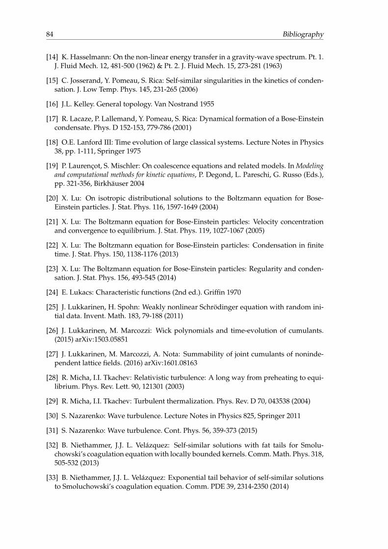
84 Bibliography

[14] K. Hasselmann: On the non-linear energy transfer in a gravity-wave spectrum. Pt. 1.J. Fluid Mech. 12, 481-500 (1962) & Pt. 2. J. Fluid Mech. 15, 273-281 (1963)

[15] C. Josserand, Y. Pomeau, S. Rica: Self-similar singularities in the kinetics of conden-sation. J. Low Temp. Phys. 145, 231-265 (2006)

[16] J.L. Kelley. General topology. Van Nostrand 1955

[17] R. Lacaze, P. Lallemand, Y. Pomeau, S. Rica: Dynamical formation of a Bose-Einsteincondensate. Phys. D 152-153, 779-786 (2001)

[18] O.E. Lanford III: Time evolution of large classical systems. Lecture Notes in Physics38, pp. 1-111, Springer 1975

[19] P. Laurencot, S. Mischler: On coalescence equations and related models. In Modelingand computational methods for kinetic equations, P. Degond, L. Pareschi, G. Russo (Eds.),pp. 321-356, Birkhauser 2004

[20] X. Lu: On isotropic distributional solutions to the Boltzmann equation for Bose-Einstein particles. J. Stat. Phys. 116, 1597-1649 (2004)

[21] X. Lu: The Boltzmann equation for Bose-Einstein particles: Velocity concentrationand convergence to equilibrium. J. Stat. Phys. 119, 1027-1067 (2005)

[22] X. Lu: The Boltzmann equation for Bose-Einstein particles: Condensation in finitetime. J. Stat. Phys. 150, 1138-1176 (2013)

[23] X. Lu: The Boltzmann equation for Bose-Einstein particles: Regularity and conden-sation. J. Stat. Phys. 156, 493-545 (2014)

[24] E. Lukacs: Characteristic functions (2nd ed.). Griffin 1970

[25] J. Lukkarinen, H. Spohn: Weakly nonlinear Schrodinger equation with random ini-tial data. Invent. Math. 183, 79-188 (2011)

[26] J. Lukkarinen, M. Marcozzi: Wick polynomials and time-evolution of cumulants.(2015) arXiv:1503.05851

[27] J. Lukkarinen, M. Marcozzi, A. Nota: Summability of joint cumulants of noninde-pendent lattice fields. (2016) arXiv:1601.08163

[28] R. Micha, I.I. Tkachev: Relativistic turbulence: A long way from preheating to equi-librium. Phys. Rev. Lett. 90, 121301 (2003)

[29] R. Micha, I.I. Tkachev: Turbulent thermalization. Phys. Rev. D 70, 043538 (2004)

[30] S. Nazarenko: Wave turbulence. Lecture Notes in Physics 825, Springer 2011

[31] S. Nazarenko: Wave turbulence. Cont. Phys. 56, 359-373 (2015)

[32] B. Niethammer, J.J. L. Velazquez: Self-similar solutions with fat tails for Smolu-chowski’s coagulation equation with locally bounded kernels. Comm. Math. Phys. 318,505-532 (2013)

[33] B. Niethammer, J.J. L. Velazquez: Exponential tail behavior of self-similar solutionsto Smoluchowski’s coagulation equation. Comm. PDE 39, 2314-2350 (2014)

Bibliography 85

[34] L.W. Nordheim: On the kinetic method in the new statistics and its application inthe electron theory of conductivity. Proc. R. Soc. London Ser. A 119, 689-698 (1928)

[35] R. Peierls: Zur kinetischen Theorie der Warmeleitung in Kristallen. Ann. Phys. 395,1055-1101 (1929)

[36] Y. Pomeau: Asymptotic time behaviour of nonlinear classical field equations. Non-linearity 5, 707-720 (1992)

[37] M. Pulvirenti, C. Saffirio, S. Simonella: On the validity of the Boltzmann equationfor short range potentials. Rev. Math. Phys. 26, 1450001 (2014)

[38] D.V. Semikoz, I.I. Tkachev: Kinetics of Bose condensation. Phys. Rev. Lett. 74, 3093-3097 (1995)

[39] D.V. Semikoz, I.I. Tkachev: Condensation of bosons in the kinetic regime. Phys. Rev.D 55, 489-502 (1997)

[40] H. Spohn: Kinetics of the Bose-Einstein condensation. Phys. D 239, 627-634 (2010)

[41] C. Sulem, P.-L. Sulem: The nonlinear Schrodinger equation: Self-focusing and wavecollapse. Springer 1999

[42] H. Triebel: Interpolation theory, function spaces, differential operators. North-Hol-land 1978

[43] H. Triebel: Theory of function spaces. Birkhauser 1983

[44] V.E. Zakharov: Weak-turbulence spectrum in a plasma without a magnetic field. Zh.Eksp. Teor. Fiz. 51, 688-696 (1967) [Sov. Phys. JEPT 24, 455-459 (1967)]

[45] V.E. Zakharov: Collapse of Langmuir waves. Zh. Eksp. Teor. Fiz. 62, 1745-1759 (1972)[Sov. Phys. JEPT 35, 908-914 (1972)]

[46] V.E. Zakharov, N.N. Filonenko: Energy spectrum for stochastic oscillations of a fluidsurface. Dokl. Acad. Nauka SSSR 170, 1292-1295 (1966) [Sov. Phys. Dokl. 11, 881-884(1967)]

[47] V.E. Zakharov, N.N. Filonenko: Weak turbulence of capillary waves. Zh. Prikl.Mekh. Tekh. Fiz. 8(5), 62-67 (1967) [J. Appl. Mech. Tech. Phys. 8(5), 37-40 (1967)]

[48] V.E. Zakharov, V.S. L’vov, G. Falkovich: Kolmogorov spectra of turbulence I. Waveturbulence. Springer 1992

on a kinetic equation arising in weak turbulence theory

Documents