On Actively Closing Loops in Grid-based FastSLAM

Cyrill Stachniss1 Dirk Hahnel1,2 Wolfram Burgard1 Giorgio Grisetti1,3

1University of Freiburg, Department of Computer Science, D-79110 Freiburg, Germany

2Intel Research Seattle, 1100 NE 45th Street, Seattle, WA 98105, USA

3Dipartimento Informatica e Sistemistica, Universita “La Sapienza”, I-00198 Rome, Italy

Correspondence author: Cyrill Stachniss, stachnis@informatik.uni-freiburg.de

Abstract

Acquiring models of the environment belongs to the fundamental tasks of mobile robots. In

the past, several researchers have focused on the problem of simultaneous localization and mapping

(SLAM). Classical SLAM approaches are passive in the sense that they only process the perceived

sensor data and do not influence the motion of the mobile robot. In this paper, we present a

novel integrated approach that combines autonomous exploration with simultaneous localization

and mapping. Our method uses a grid-based version of the FastSLAM algorithm and considers

at each point in time actions to actively close loops during exploration. By re-entering already

visited areas, the robot reduces its localization error and in this way learns more accurate maps.

Experimental results presented in this paper illustrate the advantage of our method over previous

approaches that lack the ability to actively close loops.

keywords: exploration, active loop-closure, place re-visiting, re-localization, FastSLAM

1 Introduction

In general, the task of acquiring models of unknown environments requires the solution of three sub-

tasks, which are mapping, localization, and motion control. Mapping is the problem of integrating the

information gathered with the robot’s sensors into a given representation. Localization is the problem

of estimating the position of the robot. Finally, the motion control problem involves the question of

how to steer a vehicle in order to efficiently guide it to a desired location or along a planned trajectory.

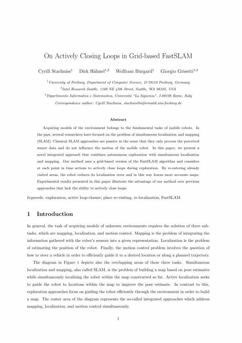
The diagram in Figure 1 depicts also the overlapping areas of these three tasks. Simultaneous

localization and mapping, also called SLAM, is the problem of building a map based on pose estimates

while simultaneously localizing the robot within the map constructed so far. Active localization seeks

to guide the robot to locations within the map to improve the pose estimate. In contrast to this,

exploration approaches focus on guiding the robot efficiently through the environment in order to build

a map. The center area of the diagram represents the so-called integrated approaches which address

mapping, localization, and motion control simultaneously.

1

activelocalization

integratedapproaches

exploration

motion control

mapping localization

SLAM

Figure 1: Sub-tasks that need to be solved by a robot in order to acquire accurate models of the

environment [14]. The overlapping areas represent combinations of these sub-tasks.

start start

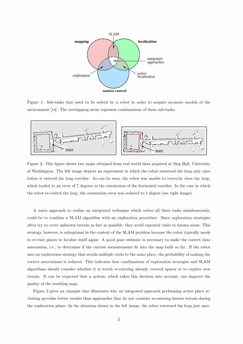
Figure 2: This figure shows two maps obtained from real world data acquired at Sieg Hall, University

of Washington. The left image depicts an experiment in which the robot traversed the loop only once

before it entered the long corridor. As can be seen, the robot was unable to correctly close the loop,

which leaded to an error of 7 degrees in the orientation of the horizontal corridor. In the case in which

the robot re-visited the loop, the orientation error was reduced to 1 degree (see right image).

A naive approach to realize an integrated technique which solves all three tasks simultaneously,

could be to combine a SLAM algorithm with an exploration procedure. Since exploration strategies

often try to cover unknown terrain as fast as possible, they avoid repeated visits to known areas. This

strategy, however, is suboptimal in the context of the SLAM problem because the robot typically needs

to re-visit places to localize itself again. A good pose estimate is necessary to make the correct data

association, i.e., to determine if the current measurements fit into the map built so far. If the robot

uses an exploration strategy that avoids multiple visits to the same place, the probability of making the

correct associations is reduced. This indicates that combinations of exploration strategies and SLAM

algorithms should consider whether it is worth re-entering already covered spaces or to explore new

terrain. It can be expected that a system, which takes this decision into account, can improve the

quality of the resulting map.

Figure 2 gives an example that illustrates why an integrated approach performing active place re-

visiting provides better results than approaches that do not consider re-entering known terrain during

the exploration phase. In the situation shown in the left image, the robot traversed the loop just once.

2

The robot was not able to correctly determine the angle between the loop and the straight corridor

because it did not collect enough data to accurately localize itself. The second map shown in the right

image has been obtained with the approach described in this paper after the robot traveled twice around

the loop before entering the corridor. As can be seen from the figure, this reduces the orientation error

from approximately 7 degrees (left image) to 1 degree (right image). This example illustrates that the

capability to actively close loops during exploration allows the robot to reduce its pose uncertainty

during exploration and thus to learn more accurate maps.

The contribution of this paper is an integrated algorithm for generating trajectories to actively

close loops during SLAM and exploration. Our algorithm uses a grid-based version of the FastSLAM

algorithm and maintains a Rao-Blackwellized particle filter to estimate the map and the trajectory of

the robot. Our approach explicitely takes into account the uncertainty about the pose of the robot

during the exploration task. Additionally, it reduces the risk that the robot becomes overly confident

in its pose when actively closing loops, which is a typical problem of particle filters in this context. As

a result, we obtain more accurate maps compared to combinations of SLAM with greedy exploration.

This paper is organized as follows. The next section discusses related work and in Section 3 we

then explain the idea of grid-based FastSLAM, the mapping algorithm used throughout this work. In

Section 4, we present our integrated exploration technique. We describe how to take into account the

pose uncertainty and how to actively close loops. Finally, Section 5 presents experiments carried out on

real robots as well as in simulation.

2 Related Work

Several previous approaches to SLAM and mobile robot exploration are related to our work. In the

context of exploration, most of the techniques presented so far focus on generating motion commands

that minimize the time needed to cover the whole terrain [2, 12, 23, 24]. Other methods seek to optimize

the view-points of the robot to maximize the expected information gain and to minimize the uncertainty

of the robot about grid cells [8, 20]. Most of these techniques, however, assume that the location of the

robot is known during exploration. In the area of SLAM, the vast majority of papers focuses on the

aspect of state estimation as well as belief representation and update [4, 5, 6, 10, 11, 15, 17, 21]. These

techniques, however, are passive and only consume incoming sensor data without explicitely generating

controls.

Recently, some techniques have been proposed which actively control the robot during SLAM. For

example, Makarenko et al. [14] as well as Bourgault et al. [1] extract landmarks out of laser range

scans and use an Extended Kalman Filter to solve the SLAM problem. Furthermore, they introduce a

utility function which trades off the cost of exploring new terrain with the utility of selected positions

with respect to a potential reduction of uncertainty. The approaches are similar to the work done by

Feder et al. [7] who consider local decisions to improve the pose estimate during mapping. Sim et

al. [19] presented an approach in which the robot follows a parametric curve to explore the environment

3

and considers place re-visiting actions if the pose uncertainty gets too high. These four techniques

integrate the uncertainty in the pose estimate of the robot into the decision process of where to move

next. However, they rely on the fact that the environment contains landmarks that can be uniquely

determined during mapping.

In contrast to this, the approach presented in this paper makes no assumptions about distinguishable

landmarks in the environment. It uses raw laser range scans to compute accurate grid maps. It considers

the utility of re-entering known parts of the environment and following an encountered loop to reduce

the uncertainty of the robot in its pose. In this way, the resulting maps become highly accurate.

3 Grid-Based FastSLAM

To estimate the map of the environment, we use a highly efficient variant of the FastSLAM algorithm [15],

which itself is an extension of the Rao-Blackwellized particle filter for simultaneous localization and

mapping proposed by Murphy et al. [5]. FastSLAM uses a set of weighted particles to represent the

full posterior p(x1:t, m | z1:t, u0:t−1) about the map m of the environment and the trajectory x1:t of the

robot given a sequence of observations z1:t up to time t and the odometry measurements u0:t−1. The

key idea of the Rao-Blackwellized particle filter for SLAM is to separate the estimation of the trajectory

of the robot from the map estimation process

p(x1:t, m | z1:t, u0:t−1) = p(x1:t | z1:t, u0:t−1)p(m | x1:t, z1:t, u0:t−1) (1)

= p(x1:t | z1:t, u0:t−1)p(m | x1:t, z1:t), (2)

where Eq. (2) is obtained from Eq. (1) by assuming that m is independent of the odometry measurements

u0:t−1 given all the poses x1:t of the robot and the corresponding observations z1:t.

To estimate the first term of Eq. (2), namely the posterior p(x1:t | z1:t, u0:t−1), FastSLAM uses a

particle filter. This filter estimates the trajectory of the robot based on the odometry information and

the observed laser range data similar to Monte-Carlo localization [3].

Estimating the full posterior about the map and poses of the robot can be done efficiently since

the quantity p(m | x1:t, z1:t) can be computed analytically once x1:t and z1:t are known. By assuming

that laser range finders provide accurate range observations and given one knows the poses of the robot

while obtaining these observations, a grid map can be directly computed using ray-casting operations.

As a result, each of the samples represents a possible trajectory of the robot and additionally maintains

an individual map which is updated upon “mapping with known poses” [16] according to its own pose

estimate.

One of the most common particle filtering algorithms is the Sampling Importance Resampling (SIR)

filter. FastSLAM incrementally processes the observations and the odometry readings as they are

available and updates the set of samples representing the posterior about the map and the trajectory of

the vehicle. The overall process can be summarized by the following four steps:

4

map of particle 2 map of particle 3map of particle 1

3 particles and their trajectories

alignmenterrors

alignmenterror

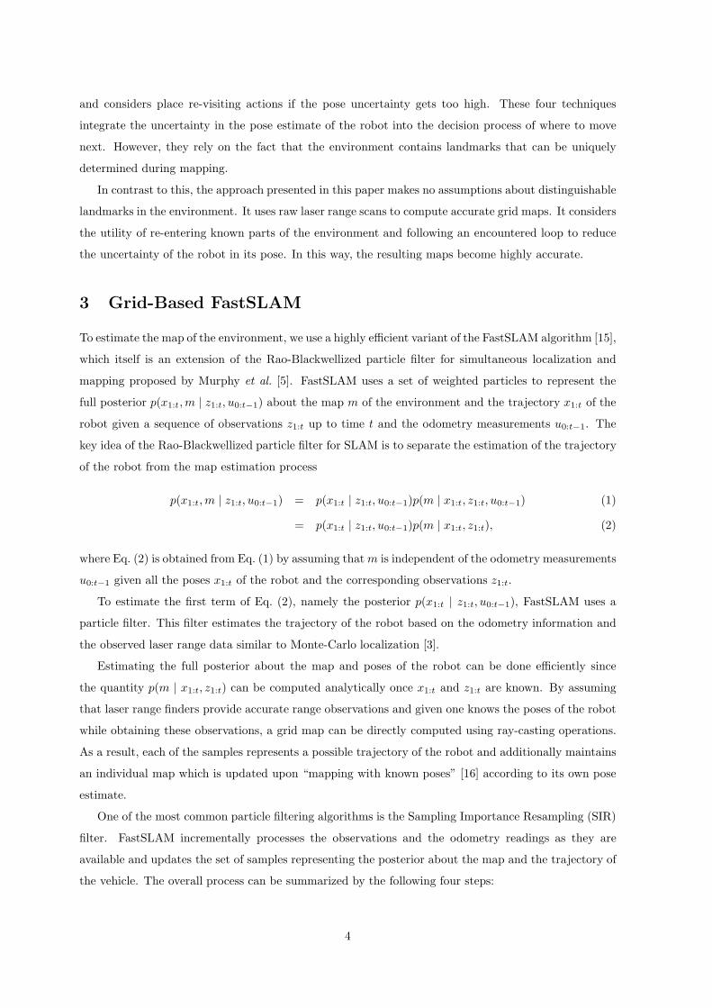
Figure 3: Example for three particles used within FastSLAM to represent p(x1:t, m | z1:t, u0:t−1). Each

particle estimates the trajectory of the robot and maintains an individual map which is updated accord-

ing to the estimated trajectory.

1. Sampling: The next generation of particles is obtained from the current generation, by sampling

from a proposal distribution π. The motion model of the robot is often used as the proposal.

2. Importance Weighting: An individual importance weight ω is assigned to each particle. The

weights account for the fact that the proposal distribution π in general is not equal to the true

distribution of successor states. In our filter, the weight of each particle is proportional to the

likelihood p(zt | m, xt) of the most recent observation given the map m associated with this particle

and the corresponding pose xt.

3. Resampling: Particles with a low importance weight ω are typically replaced by samples with a

high weight. This step is necessary since only a finite number of particles are used to approximate

a continuous distribution. Furthermore, resampling allows to apply a particle filter in situations

in which the true distribution differs from the proposal.

4. Map Estimating: For each particle, the corresponding map estimate is updated based on the

obtained observation and the pose represented by that particle.

The FastSLAM algorithm used throughout this paper computes grid maps. It applies a scan-

matching procedure to compute highly accurate odometry data and uses this corrected odometry in

the prediction step of the particle filter [11]. In this way, the number of particles can be reduced so that

even maps of large environments can be constructed online. An example for such a filter is illustrated in

Figure 3. It depicts three particles with the individually estimated trajectories and the maps updated

according to the estimated trajectory. In the depicted situation, the robot closed a loop and the dif-

ferent particles produced different maps. Particle 1 generated an quite accurate pose estimate, whereas

5

particles 3 yields big alignments errors. Therefore, particle 1 will get a much higher importance weight

compared to particle 3. The weight of particle 2 will by between the weight of particle 1 and 3 because

its alignment error is smaller than the one of particle 3 but bigger than the one of particle 1.

Note that adapting the map discretization leads to only minor changes in the resulting trajectory.

Generally, the finer the resolution, the more precise is typically the pose estimate and therefore the

resulting map. However, our observation is that as long as the grid resolution is reasonable small, it

mainly influences the execution time of the algorithm and the memory requirements. Typically, the grid

resolution is set values between 5cm and 15cm.

In the following section, we describe how to actively close loops during exploration in order to obtain

accurate grid maps using the FastSLAM algorithm.

4 Exploration With Active Loop-Closing for FastSLAM

During FastSLAM, whenever the robot explores new terrain, all samples have more or less the same

importance weight, since the most recent measurement is typically consistent with the part of the map

constructed from the immediately preceding observations. As a result, the uncertainty of the particle

filter increases. As soon as it re-enters known terrain, however, the maps of some particles are consistent

with the current measurement and some are not. Accordingly the weights of the samples differ largely.

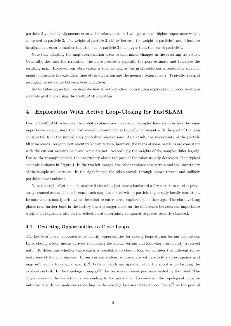
Due to the resampling step, the uncertainty about the pose of the robot usually decreases. One typical

example is shown in Figure 4. In the two left images, the robot explores new terrain and the uncertainty

of the sample set increases. In the right image, the robot travels through known terrain and unlikely

particles have vanished.

Note that this effect is much smaller if the robot just moves backward a few meters to re-visit previ-

ously scanned areas. This is because each map associated with a particle is generally locally consistent.

Inconsistencies mostly arise when the robot re-enters areas explored some time ago. Therefore, visiting

places seen further back in the history has a stronger effect on the differences between the importance

weights and typically also on the reduction of uncertainty compared to places recently observed.

4.1 Detecting Opportunities to Close Loops

The key idea of our approach is to identify opportunities for closing loops during terrain acquisition.

Here, closing a loop means actively re-entering the known terrain and following a previously traversed

path. To determine whether there exists a possibility to close a loop we consider two different repre-

sentations of the environment. In our current system, we associate with particle s an occupancy grid

map m[s] and a topological map G[s], both of which are updated while the robot is performing the

exploration task. In the topological map G[s], the vertices represent positions visited by the robot. The

edges represent the trajectory corresponding to the particle s. To construct the topological map, we

initialize it with one node corresponding to the starting location of the robot. Let x[s]t

be the pose of

6

s*

s*

s*

Figure 4: Evolution of a particle set and the map of the particle s∗ at three different time steps. In

the two left images, the vehicle traveled through unknown terrain, so that the uncertainty increased. In

the right image, the robot re-entered known terrain so that samples representing unlikely trajectories

vanished.

particle s at the current time step t. We add a new node at x[s]t to G[s] if the distance between x

[s]t and

all other nodes in G[s] exceeds a threshold c (here set to 2.5m) or if none of the other nodes in G[s] is

visible from x[s]t :

∀n ∈ nodes(G[s]) :[

distm[s](x[s]t

, n) > c ∨ not visiblem[s](x[s]t

, n)]

. (3)

Whenever a new node is created, we also add an edge from this node to the most recently visited node.

To determine whether or not a node is visible from another node, we perform a ray-casting operation

in the occupancy grid m[s].

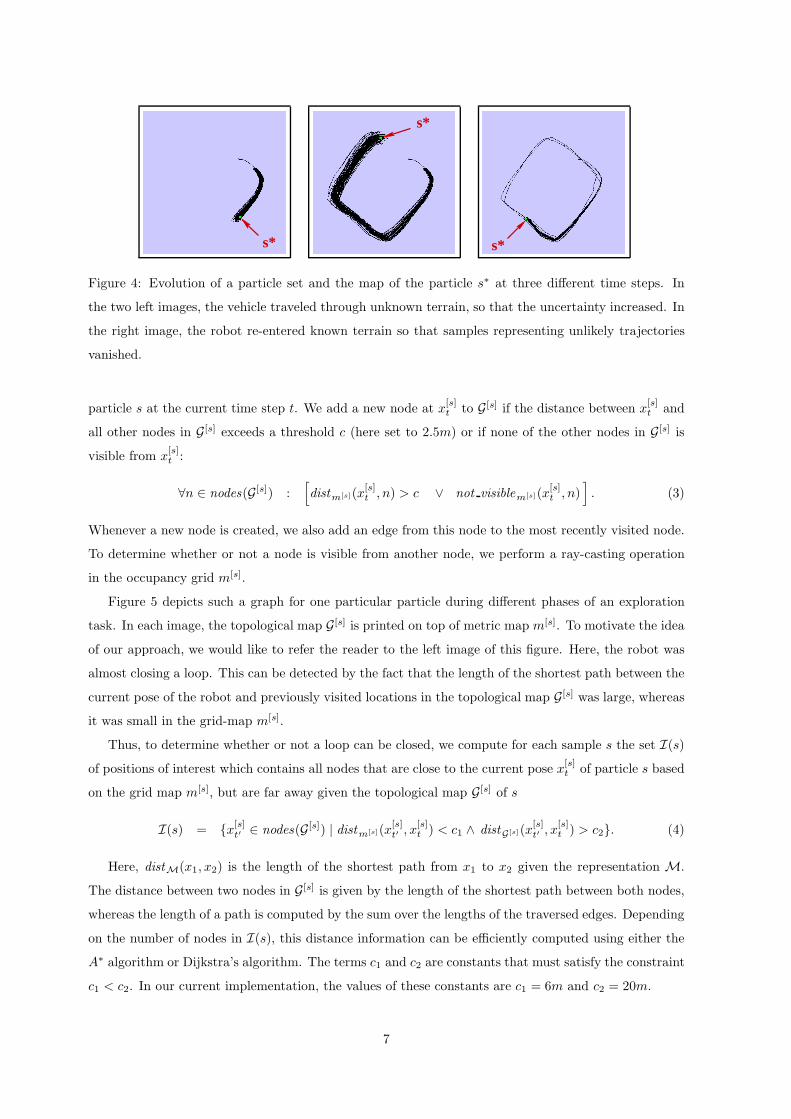
Figure 5 depicts such a graph for one particular particle during different phases of an exploration

task. In each image, the topological map G[s] is printed on top of metric map m[s]. To motivate the idea

of our approach, we would like to refer the reader to the left image of this figure. Here, the robot was

almost closing a loop. This can be detected by the fact that the length of the shortest path between the

current pose of the robot and previously visited locations in the topological map G[s] was large, whereas

it was small in the grid-map m[s].

Thus, to determine whether or not a loop can be closed, we compute for each sample s the set I(s)

of positions of interest which contains all nodes that are close to the current pose x[s]t of particle s based

on the grid map m[s], but are far away given the topological map G[s] of s

I(s) = {x[s]t′∈ nodes(G[s]) | distm[s](x

[s]t′

, x[s]t ) < c1 ∧ distG[s](x

[s]t′

, x[s]t ) > c2}. (4)

Here, distM(x1, x2) is the length of the shortest path from x1 to x2 given the representation M.

The distance between two nodes in G[s] is given by the length of the shortest path between both nodes,

whereas the length of a path is computed by the sum over the lengths of the traversed edges. Depending

on the number of nodes in I(s), this distance information can be efficiently computed using either the

A∗ algorithm or Dijkstra’s algorithm. The terms c1 and c2 are constants that must satisfy the constraint

c1 < c2. In our current implementation, the values of these constants are c1 = 6m and c2 = 20m.

7

x[s]t

6

I(s)���

?x

[s]t

��

x[s]t

-

Figure 5: The red dots and lines in these three image represent the nodes and edges of G[s]. In the left

image, I(s) contained two nodes (indicated by the arrows) and in the middle image the robot closed

the loop until the pose uncertainty is reduced. After this, it continued with the acquisition of unknown

terrain (right image).

If I(s) 6= ∅, there exist so-called shortcuts from the current pose x[s]t represented by the correspond-

ing particle to the positions in I(s). These shortcuts represent edges that would close a loop in the

topological map G[s]. The left image of Figure 5 illustrates a situation in which a robot encounters the

opportunity to close a loop since I(s) contains two nodes which is indicated by two arrows. The key

idea of our approach is to use such shortcuts whenever the uncertainty of the robot in its pose becomes

too large. The robot then re-visits portions of the previously explored area and in this way reduces the

uncertainty in its position.

To determine the most likely movement allowing the robot to follow a previous path of a loop, one in

principle has to integrate over all particles and consider all potential outcomes of that particular action.

Since this would be too time consuming for online-processing, we consider only the particle s∗ with the

highest accumulated logarithmic observation likelihood:

s∗ = argmaxs

t∑

i=1

log p(zi midm[s], x[s]i

). (5)

If I(s∗) 6= ∅, we choose the node xtefrom I(s∗) which is closest to x

[s∗]t

xte= argmin

x∈I(s∗)

distm[s∗](x[s∗]t

, x). (6)

In the sequel, xteis denoted as the entry point at which the robot has the possibility to close a loop. te

corresponds to the last time the robot was at the node xte.

Note that it can happen that the particle s∗ is far away from representing the correct pose estimate.

In such a situation, the robot sometimes computes a path, which cannot be traversed in practice. The

robot will follow this path until it recognizes that it is blocked and then will abort the loop closing

behavior.

8

Figure 6: The particle depletion problem: A robot traveled through the inner loop several times (left

image). After this, the diversity of hypotheses about the trajectory outside the inner loop had decreased

too much (middle image) and the robot is unable to close the outer loop correctly (right image).

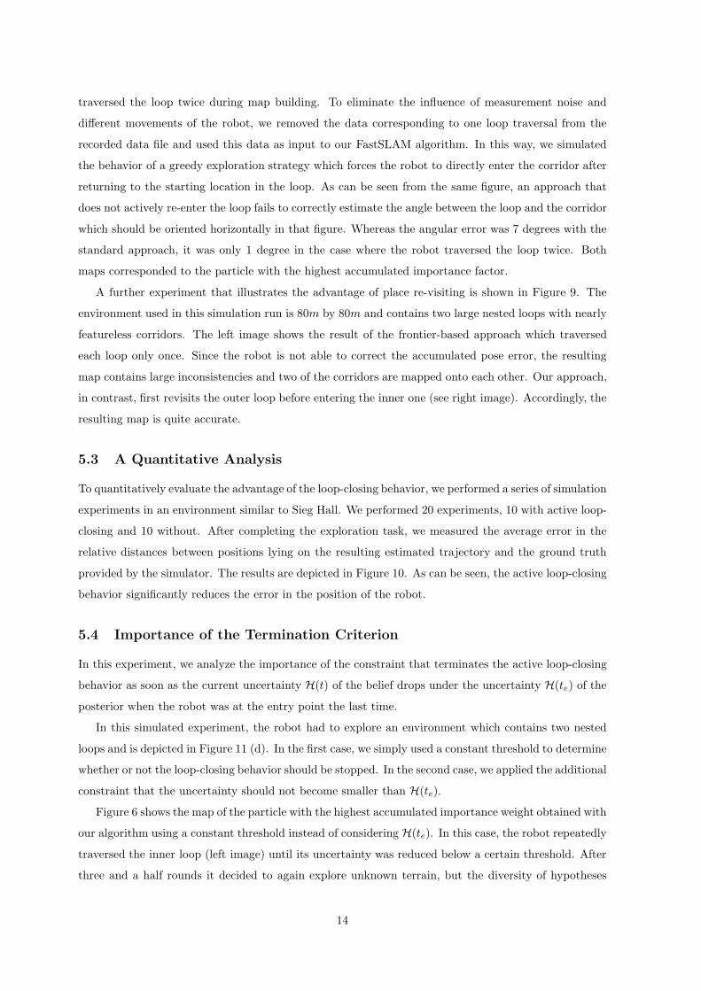
4.2 Stopping the Loop-Closing Process

To determine whether or not the robot should activate the loop-closing behavior, our system constantly

monitors the uncertainty H(t) about the robot’s pose at the current time step. The necessary condition

for starting the loop-closing process is the existence of an entry point xteand that H(t) exceeds a given

threshold. Once the loop-closing process has been activated, the robot approaches xteand then follows

the path taken after previously arriving at xte. During this process, the uncertainty in the pose of the

vehicle typically decreases because the robot is able to localize itself in the map built so far and unlikely

particles vanish.

Furthermore, we have to define a criterion for deciding when the robot actually has to stop following

a loop. A first attempt could be to introduce a threshold and to simply stop the trajectory following

behavior as soon as the uncertainty becomes smaller than a given threshold. This criterion, however, can

be problematic especially in the case of nested loops. Suppose the robot encounters the opportunity to

close a loop that is nested within an outer and so far unclosed loop. If it eliminates all of its uncertainty

by repeatedly traversing the inner loop, particles necessary to close the outer loop may vanish. As a

result, the filter diverges and the robot fails to build a correct map (compare Figure 6).

To remedy this so-called particle depletion problem [22], we introduce a constraint on the uncertainty

of the robot. Let H(te) denote the uncertainty of the posterior when the robot visited the entry point

last time. Then the new constraint allows the robot to re-traverse the loop only as long as its current

uncertainty H(t) exceeds H(te). If the constraint is violated the robot resumes its terrain acquisition

(exploration) process. This constraint is designed to reduce the risk of depleting relevant particles during

the loop-closing process. The idea is that by observing the area within the loop, the robot does not

obtain any information about the world outside the loop. As a result, the robot cannot reduce the

uncertainty H(t) in its current posterior below its uncertainty H(te) when entering the loop since H(te)

is the uncertainty stemming from the world outside the loop.

To better illustrate the importance of this constraint, consider the following example: A robot moves

9

from place A to place B and then repeatedly observes B. While it is mapping B, it does not get any

further information about A. Since each particle represents a whole trajectory of the robot, hypotheses

representing ambiguities about A will also vanish when reducing potential uncertainties about B. Our

constraint reduces the risk of depleting particles representing ambiguities about A by aborting the

loop-closing behavior at B as soon as the uncertainty drops below the uncertainty stemming from A.

Finally, we have to describe how we actually measure the uncertainty in the position estimate. The

typical way of measuring the uncertainty of a posterior is to use the entropy. To compute the entropy

of a posterior represented by particles, one typically uses a multi-dimensional grid representing the

possible (discretized) states. Each cell a in this grid stores a probability which is given by the sum of

the normalized weights of the samples corresponding to that cell. The entropy is then computed by

summing up −p(a) log p(a) of each cell a in that grid.

In the case of multi-modal distributions, however, the entropy does not consider the distance between

the different modes. As a result, a set of k different pose hypotheses which are located close by each other

leads to the same entropy value than the situation in which k hypotheses are randomly distributed over

the environment. The resulting maps, however, would look similar in the first case, but quite different

in the second case. In our experiments, we figured out that we obtain better results if we use the

volume expanded by the samples instead of the entropy of the posterior. We therefore calculate the

pose uncertainty by determining the volume of the oriented bounding box around the particle cloud.

A good approximation of the minimal oriented bounding box can be obtained efficiently by a principal

component analysis.

Note that the loop-closing process is also aborted after a robot traveled for a long period of time

in the same loop in order to avoid a – theoretically possible – endless loop-closing behavior. In all our

experiments, however, this problem has never been encountered.

4.3 Reducing the Exploration Time

The experiments presented later on in this paper demonstrate that our uncertainty based stopping

criterion is an effective way to reduce the risk of particle depletion. However, it can happen that newly

acquired sensor data acquired during loop-closing does not provide a lot of new information for the

robot. Moving through such terrain leads to an increased exploration time. Therefore, it would be more

efficient to abort the loop-closing in situations in which the new sensor data does not help to identify

unlikely hypotheses.

To estimate how well the current set of N particle represents the true posterior, Liu [13] introduced

the effective number of particles Neff (also called effective sample size):

Neff (t) =1

∑N

s=1

(

ω[s]t

)2 (7)

The idea behind this measure is to determine the variance in the importance weights of the particles.

Liu uses Neff to resample in an intelligent way but it is also useful in the context of active loop-

10

closing. We monitor the change of Neff over time, which allows us to analyze how the new acquired

information affects the filter. If Neff stays constant, the new information does not help to identify

unlikely hypotheses represented by the individual particles. In that case, the variance in the importance

weights of the particles does not change over time. If, in contrast, the value of Neff decreases over time,

the new information is used to identify that some particles are less likely than others. This is exactly

the criterion we need to decide whether or not the loop-closing should be aborted in order to keep the

exploration time small. As long as new information helps to identify unlikely particles, we follow the

loop. As soon as the observations do not provide any new knowledge about the environment for a period

of k time steps, we continue to explore new terrain.

Note that this criterion is optional and in not essential for a successful loop-closing strategy. It

can directly be used if the underlying FastSLAM approach applies an adaptive resampling technique 1.

More details on Rao-Blackwellized mapping using adaptive resampling have been published by Grisetti

et al. [9]. In the experimental section of this paper, we will demonstrate that Neff is a useful criterion

in the context of active loop-closing and how it behaves during exploration.

As long as the robot is localized well enough or no loop can be closed, we use a frontier-based

exploration strategy [2] to choose target points for the robot. A frontier is any known and unoccupied

cell that is an immediate neighbor of an unknown, unexplored cell [24]. By extracting frontiers from

a given grid map, one can easily determine potential target locations which lead the robot to so far

unknown terrain. To select one of these frontier cells as the next goal location, a common way is to

determine the travel cost to each frontier cell. This cost can be computed using Dijkstra’s algorithm

or a value iteration technique like done in [2]. It has been shown by Koenig and Tovey [12], that for

a single robot this strategy yields reasonable short trajectories compared to the theoretically optimal

solution. In our current system, we determine frontiers based on the map of the particle s∗.

A precise formulation of the loop-closing strategy is given by Algorithm 1. In our implementation, this

algorithm runs as a background process that is able interrupt the frontier-based exploration procedure.

1: Compute I(s∗)

2: if I(s∗) 6= ∅ then begin

3: H ← H(te)

4: path ← x[s∗]t· shortest pathG[s∗](xte

, x[s∗]t

)

5: while H(t) > H ∧ var(Neff (n− k), . . . , Neff (n)) > ǫ do

6: robot follow(path)

7: end

Algorithm 1: The loop-closing algorithm

1If no adaptive resampling is used, one needs to monitor the relative change in Neff after integrating each measurements,

because after each resampling step the weights of all particles are set to 1

N. As a result, Neff is always equal to the number

N of particles and the variance therefore is zero.

11

start

Figure 7: Active loop-closing of multiple nested loops.

4.4 Handling Multiple Nested Loops

Note that our loop-closing technique can also handle multiple nested loops. During the loop-closing

process, the robot follows its previously taken trajectory to re-localize. It does not leave this trajectory

until the termination criterion (see line 5 in Algorithm 1) is fulfilled. Therefore, it never starts a new

loop-closing process before the current one is completed. A typical example with multiple nested loops is

illustrated in Figure 7. In the situation depicted in the left picture, the robot starts with the loop-closing

process for the inner loop. After completing the most inner loop, it moves to the second inner one and

again starts the loop-closing process. Since our algorithm considers the uncertainty at the entry point,

it keeps enough variance in the filter to also close the outer loop correctly. In general, the quality of

the solution and whether or not the overall process succeeds depends on the number of particles used.

Since determining this quantity is an open research problem, the number of particles has to be defined

by the user in our current system.

5 Experiments

Our approach has been implemented and evaluated in a series of real world and simulation experiments.

For the real world experiments we used an iRobot B21r robot and an ActivMedia Pioneer II robot.

Both are equipped with a SICK laser range finder. For the simulation experiments we used the real-

time simulator of the Carnegie Mellon Robot Navigation Toolkit [18].

The experiments described in this section are designed to illustrate that our approach can be used

to actively learn accurate maps of large indoor environments. Furthermore, they demonstrate that our

integrated approach yields better results than an approach without active loop-closing. Additionally,

we analyze how the active termination of the loop-closure influences the result of the mapping process.

5.1 Real World Exploration

The first experiment was carried out to illustrate that our current system can effectively control a mobile

robot to actively close loops during exploration. To perform this experiment, we used a Pioneer II robot

to explore the main lobby of the Department for Computer Science at the University of Freiburg. The

12

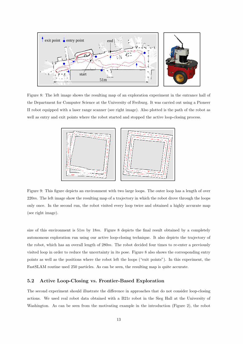
51m

exit point entry point end

start

Figure 8: The left image shows the resulting map of an exploration experiment in the entrance hall of

the Department for Computer Science at the University of Freiburg. It was carried out using a Pioneer

II robot equipped with a laser range scanner (see right image). Also plotted is the path of the robot as

well as entry and exit points where the robot started and stopped the active loop-closing process.

Figure 9: This figure depicts an environment with two large loops. The outer loop has a length of over

220m. The left image show the resulting map of a trajectory in which the robot drove through the loops

only once. In the second run, the robot visited every loop twice and obtained a highly accurate map

(see right image).

size of this environment is 51m by 18m. Figure 8 depicts the final result obtained by a completely

autonomous exploration run using our active loop-closing technique. It also depicts the trajectory of

the robot, which has an overall length of 280m. The robot decided four times to re-enter a previously

visited loop in order to reduce the uncertainty in its pose. Figure 8 also shows the corresponding entry

points as well as the positions where the robot left the loops (“exit points”). In this experiment, the

FastSLAM routine used 250 particles. As can be seen, the resulting map is quite accurate.

5.2 Active Loop-Closing vs. Frontier-Based Exploration

The second experiment should illustrate the difference in approaches that do not consider loop-closing

actions. We used real robot data obtained with a B21r robot in the Sieg Hall at the University of

Washington. As can be seen from the motivating example in the introduction (Figure 2), the robot

13

traversed the loop twice during map building. To eliminate the influence of measurement noise and

different movements of the robot, we removed the data corresponding to one loop traversal from the

recorded data file and used this data as input to our FastSLAM algorithm. In this way, we simulated

the behavior of a greedy exploration strategy which forces the robot to directly enter the corridor after

returning to the starting location in the loop. As can be seen from the same figure, an approach that

does not actively re-enter the loop fails to correctly estimate the angle between the loop and the corridor

which should be oriented horizontally in that figure. Whereas the angular error was 7 degrees with the

standard approach, it was only 1 degree in the case where the robot traversed the loop twice. Both

maps corresponded to the particle with the highest accumulated importance factor.

A further experiment that illustrates the advantage of place re-visiting is shown in Figure 9. The

environment used in this simulation run is 80m by 80m and contains two large nested loops with nearly

featureless corridors. The left image shows the result of the frontier-based approach which traversed

each loop only once. Since the robot is not able to correct the accumulated pose error, the resulting

map contains large inconsistencies and two of the corridors are mapped onto each other. Our approach,

in contrast, first revisits the outer loop before entering the inner one (see right image). Accordingly, the

resulting map is quite accurate.

5.3 A Quantitative Analysis

To quantitatively evaluate the advantage of the loop-closing behavior, we performed a series of simulation

experiments in an environment similar to Sieg Hall. We performed 20 experiments, 10 with active loop-

closing and 10 without. After completing the exploration task, we measured the average error in the

relative distances between positions lying on the resulting estimated trajectory and the ground truth

provided by the simulator. The results are depicted in Figure 10. As can be seen, the active loop-closing

behavior significantly reduces the error in the position of the robot.

5.4 Importance of the Termination Criterion

In this experiment, we analyze the importance of the constraint that terminates the active loop-closing

behavior as soon as the current uncertainty H(t) of the belief drops under the uncertainty H(te) of the

posterior when the robot was at the entry point the last time.

In this simulated experiment, the robot had to explore an environment which contains two nested

loops and is depicted in Figure 11 (d). In the first case, we simply used a constant threshold to determine

whether or not the loop-closing behavior should be stopped. In the second case, we applied the additional

constraint that the uncertainty should not become smaller than H(te).

Figure 6 shows the map of the particle with the highest accumulated importance weight obtained with

our algorithm using a constant threshold instead of considering H(te). In this case, the robot repeatedly

traversed the inner loop (left image) until its uncertainty was reduced below a certain threshold. After

three and a half rounds it decided to again explore unknown terrain, but the diversity of hypotheses

14

0

0.5

1

1.5

2

2.5

loop-closing frontiers

avg.

err

or in

pos

ition

[m]

Figure 10: This figure compares our loop-closing strategy with a pure frontier-based exploration tech-

nique. The left bar in this graph plots the average error in the pose of the robot obtained with our

loop-closing strategy. The right one shows the average error when a frontier-based approach was used.

As can be seen, our technique significantly reduces the distances between the estimated positions and

the ground truth (confidence intervals do not overlap).

had decreased too much (middle image). Accordingly the robot was unable to accurately close the

outer loop (right image). We repeated this experiment several times and in none of the cases was the

robot able to correctly map the environment. In contrast, our approach using the additional constraint

always generated an accurate map. One example is shown in Figure 11. Here, the robot stopped the

loop-closing after traversing half of the inner loop. In both cases we used 80 particles.

As this experiment illustrates, the termination of the loop-closing is important for the convergence

of the filter and to obtain accurate maps in environments with several (nested) loops. Note that similar

results in principle can also be obtained without this termination constraint if the number of particles

is dramatically increased. Since exploration is an online problem and each particle carries its own map

it is of utmost importance to keep the number of particles as small as possible. Therefore, our approach

can also be regarded as a contribution to limit the number of particles during FastSLAM.

5.5 Evolution of Neff

In this experiment, we demonstrate the behavior of the optional termination criterion that triggers the

active loop-closing behavior. Additionally to the constraint that the uncertainty H(t) must be bigger

than the uncertainty at the entry point H(te) of the loop, the process is stopped whenever the effective

number of particles Neff stays constant for a certain period of time. This criterion, which can be applied

if the underlying mapping system uses an adaptive resampling technique [9], was introduced to avoid

that the robot moves through the loop even if no new information can be obtained from the sensor data.

The robot re-traverses the loop only as long as the sensor data is useful to identify unlikely hypotheses

about maps and poses.

One typical evolution of Neff is depicted in the left image of Figure 12. To achieve a good visualization

of the evolution of Neff , we processed a recorded data file using 150 particles. Due to the adaptive

resampling strategy, only very few resampling operations were needed. The robot started at position A

15

entrypoint

(a) (b)

(c) (d)

Figure 11: In image (a), the robot detected an opportunity to close a loop. It traversed parts of the

inner loop as long as its uncertainty exceed the uncertainty H(te) of the posterior when the robot at

the entry point and started the loop-closing process. The robot then turned back and left the loop (b)

so that enough hypotheses survived to correctly close the outer loop (c) and (d). In contrast, a system

considering only a constant threshold criterion fails to map the environment correctly as depicted in

Figure 6.

25

50

75

100

A

Nef

f / N

[%

]

time index

B C

A

C

B

Figure 12: The graph plots the evolution of the Neff function over time during an experiment carried

out in the environment shown in the right image. The robot started at position A. The position B

corresponds to the closure of the inner loop, and C corresponds to closure of the outer loop.

16

and in the first part of the experiment moved through unknown terrain (between the positions A and

B). As can be seen, Neff decreases over time. After the loop has been closed correctly and unlikely

hypotheses had partly been removed by the resampling action (position B), the robot re-traversed the

inner loop and Neff stayed more or less constant. This indicates that acquiring further data in this area

has only a small effect on the relative likelihood of the particles and the system could not determine

which hypotheses represented unlikely configurations. In such a situation, it therefore makes more sense

to focus on new terrain acquisition and to not continue the loop-closing process.

Furthermore, we analyzed the length of the trajectory traveled by the robot. Due to the active loop-

closing, our technique generates longer trajectories compared to a purely frontier-based exploration

strategy. We performed several experiments in different environments in which the robot had the

opportunity to close loops and measured the average overhead. During our experiments, we observed

an overhead varying from 3% to 10%, but it obviously depends on number of loops in the environment.

5.6 Multiple Nested Loops

To illustrate, that our approach is able to deal with several nested loops, we performed a simulated

experiment shown in Figure 13. The individual images in this figure depict eight snapshots recorded

during exploration. Image (a) depicts the robot while exploring new terrain and image (b) while actively

closing the most inner loop. After that, the robot focused on acquiring so far unknown terrain and maps

the most outer loop as shown in (c) and (d). Then the robot detects a possibility to close a loop (e)

and follows its previously taken trajectory (f). After aborting the loop closing behavior, the robot again

explores the loop in the middle (g), again closes the loop accurately, and finishes the exploration task

(h).

5.7 Computational Resources

Note that our loop-closing approach needs only a few additional resources. To detect loops, we maintain

an additional topological map for each particle. These topological maps are stored as a graph structure

and for typical environments only a few kilobytes of extra memory is needed. To determine the distances

based on the grid map in Eq. (3) and (4), our approach directly re-uses the result of a value iteration

(alternatively Dijkstra’s algorithm) computed on the most likely grid map, which has already been

computed in order to evaluate the frontier cells. Only the distance computation using the topological

map needs to be done from scratch. However, since the number of nodes in the topological map is

much smaller than the number of grid cells, the computational overhead is comparably small. In our

experiments, the time to perform all computations in order to decide where to move next increased by

around 10ms on a standard PC when activation the active loop-closing technique.

17

topological map

best frontier

robot

active loop closure

loop detected active loop closure

new terrain acquisition

(a) (b) (c) (d)

(e) (f) (g) (h)

new terrain acquisition

new terrain acquisition

Figure 13: Snapshots during the exploration of a simulated environment with several nested loops. The

red circles represent nodes of the topological map plotted on top of the most likely grid map. The yellow

circle corresponds to the frontier cell the robot currently seeks to reach.

6 Conclusions

In this paper, we presented a novel approach for active loop-closing during autonomous exploration.

We combined a Rao-Blackwellized particle filter for localization and mapping with a frontier-based

exploration technique extended by the ability to actively close loops. Our algorithm forces the robot

to re-traverse previously visited loops and in this way reduces the uncertainty in the pose estimate. As

a result, we obtain more accurate maps compared to standard combinations of SLAM algorithms with

exploration techniques. As fewer particles need to be maintained to build accurate maps, our approach

can also be regarded as a contribution to limit the number of particles needed during FastSLAM.

Acknowledgment

This work has partly been supported by the German Science Foundation (DFG) under contract number

SFB/TR-8 (project A3) and by the EC under contract number FP6-004250-CoSy.

REFERENCES

[1] F. Bourgoult, A.A. Makarenko, S.B. Williams, B. Grocholsky, and F. Durrant-Whyte. Information

based adaptive robotic exploration. In Proc. of the IEEE/RSJ Int. Conf. on Intelligent Robots and

Systems (IROS), Lausanne, Switzerland, 2002.

18

[2] W. Burgard, M. Moors, C. Stachniss, and F. Schneider. Coordinated multi-robot exploration. IEEE

Transactions on Robotics, 2005. To appear.

[3] F. Dellaert, D. Fox, W. Burgard, and S. Thrun. Monte carlo localization for mobile robots. In

Proc. of the IEEE Int. Conf. on Robotics & Automation (ICRA), Leuven, Belgium, 1998.

[4] G. Dissanayake, H. Durrant-Whyte, and T. Bailey. A computationally efficient solution to the

simultaneous localisation and map building (SLAM) problem. In ICRA’2000 Workshop on Mobile

Robot Navigation and Mapping, San Francisco, CA, USA, 2000.

[5] A. Doucet, J.F.G. de Freitas, K. Murphy, and S. Russel. Rao-blackwellized partcile filtering for

dynamic bayesian networks. In Proc. of the Conf. on Uncertainty in Artificial Intelligence (UAI),

Stanford, CA, USA, 2000.

[6] A. Eliazar and R. Parr. DP-SLAM: Fast, robust simultainous localization and mapping without

predetermined landmarks. In Proc. of the Int. Conf. on Artificial Intelligence (IJCAI), Acapulco,

Mexico, 2003.

[7] H. Feder, J. Leonard, and C. Smith. Adaptive mobile robot navigation and mapping. Int. Journal

of Robotics Research, 18(7), 1999.

[8] R. Grabowski, P. Khosla, and H. Choset. Autonomous exploration via regions of interest. In Proc. of

the IEEE/RSJ Int. Conf. on Intelligent Robots and Systems (IROS), Las Vegas, NV, USA, 2003.

[9] G. Grisetti, C. Stachniss, and W. Burgard. Improving grid-based slam with rao-blackwellized

particle filters by adaptive proposals and selective resampling. In Proc. of the IEEE Int. Conf. on

Robotics & Automation (ICRA), pages 2443–2448, Barcelona, Spain, 2005.

[10] J.-S. Gutmann and K. Konolige. Incremental mapping of large cyclic environments. In Proc. of the

IEEE Int. Symposium on Computational Intelligence in Robotics and Automation (CIRA), pages

318–325, Monterey, CA, USA, 1999.

[11] D. Hahnel, W. Burgard, D. Fox, and S. Thrun. An efficient FastSLAM algorithm for generat-

ing maps of large-scale cyclic environments from raw laser range measurements. In Proc. of the

IEEE/RSJ Int. Conf. on Intelligent Robots and Systems (IROS), Las Vegas, NV, USA, 2003.

[12] S. Koenig and C. Tovey. Improved analysis of greedy mapping. In Proc. of the IEEE/RSJ

Int. Conf. on Intelligent Robots and Systems (IROS), Las Vegas, NV, USA, 2003.

[13] J.S. Liu. Metropolized independent sampling with comparisons to rejection sampling and impor-

tance sampling. Statist. Comput., 6:113–119, 1996.

[14] A.A. Makarenko, S.B. Williams, F. Bourgoult, and F. Durrant-Whyte. An experiment in integrated

exploration. In Proc. of the IEEE/RSJ Int. Conf. on Intelligent Robots and Systems (IROS),

Lausanne, Switzerland, 2002.

19

[15] M. Montemerlo, S. Thrun, D. Koller, and B. Wegbreit. FastSLAM: A factored solution to simul-

taneous localization and mapping. In Proc. of the National Conference on Artificial Intelligence

(AAAI), Edmonton, Canada, 2002.

[16] H.P. Moravec and A.E. Elfes. High resolution maps from wide angle sonar. In Proc. of the IEEE

Int. Conf. on Robotics & Automation (ICRA), pages 116–121, St. Louis, MO, USA, 1985.

[17] K. Murphy. Bayesian map learning in dynamic environments. In Neural Info. Proc. Systems (NIPS),

Denver, CO, USA, 1999.

[18] N. Roy, M. Montemerlo, and S. Thrun. Perspectives on standardization in mobile robot program-

ming. In Proc. of the IEEE/RSJ Int. Conf. on Intelligent Robots and Systems (IROS), Las Vegas,

NV, USA, 2003.

[19] R. Sim, G. Dudek, and N. Roy. Online control policy optimization for minimizing map uncertainty

during exploration. In Proc. of the IEEE Int. Conf. on Robotics & Automation (ICRA), New

Orleans, LA, USA, 2004.

[20] C. Stachniss and W. Burgard. Exploring unknown environments with mobile robots using coverage

maps. In Proc. of the Int. Conf. on Artificial Intelligence (IJCAI), pages 1127–1132, Acapulco,

Mexico, 2003.

[21] S. Thrun. An online mapping algorithm for teams of mobile robots. Int. Journal of Robotics

Research, 2001.

[22] R. van der Merwe, N. de Freitas, A. Doucet, and E. Wan. The unscented particle filter. Technical

Report CUED/F-INFENG/TR380, Cambridge University Engineering Department, August 2000.

[23] G. Weiß, C. Wetzler, and E. von Puttkamer. Keeping track of position and orientation of moving

indoor systems by correlation of range-finder scans. In Proc. of the IEEE/RSJ Int. Conf. on

Intelligent Robots and Systems (IROS), pages 595–601, Munich, Germany, 1994.

[24] B. Yamauchi. Frontier-based exploration using multiple robots. In Proc. of the Second International

Conference on Autonomous Agents, pages 47–53, Minneapolis, MN, USA, 1998.

20