on challenges in training recurrent neural networkssarathchandar.in/paper/chandar_phd_thesis.pdf ·...

Universite de Montreal

On Challenges in Training Recurrent Neural Networks

par

Sarath Chandar Anbil Parthipan

Departement d’informatique et de recherche operationnelleFaculte des arts et des sciences

These presentee a la Faculte des arts et des sciencesen vue de l’obtention du grade de Philosophiæ Doctor (Ph.D.)

en informatique

Composition du jury

President-rapporteur: Jian-Yun Nie

Directeur de recherche: Yoshua Bengio

Co-directeur: Hugo Larochelle

Membre du jury: Pascal Vincent

Examinateur externe: Alex Graves

November, 2019

Résumé

Dans un probleme de prediction a multiples pas discrets, la prediction a chaqueinstant peut dependre de l’entree a n’importe quel moment dans un passe lointain.Modeliser une telle dependance a long terme est un des problemes fondamentauxen apprentissage automatique. En theorie, les Reseaux de Neurones Recurrents(RNN) peuvent modeliser toute dependance a long terme. En pratique, puisque lamagnitude des gradients peut croıtre ou decroıtre exponentiellement avec la dureede la sequence, les RNNs ne peuvent modeliser que les dependances a court terme.Cette these explore ce probleme dans les reseaux de neurones recurrents et proposede nouvelles solutions pour celui-ci.

Le chapitre 3 explore l’idee d’utiliser une memoire externe pour stocker les etatscaches d’un reseau a Memoire Long et Court Terme (LSTM). En rendant l’operationd’ecriture et de lecture de la memoire externe discrete, l’architecture proposee reduitle taux de decroissance des gradients dans un LSTM. Ces operations discretespermettent egalement au reseau de creer des connexions dynamiques sur de longsintervalles de temps. Le chapitre 4 tente de caracteriser cette decroissance desgradients dans un reseau de neurones recurrent et propose une nouvelle architecturerecurrente qui, grace a sa conception, reduit ce probleme. L’Unite Recurrente Non-saturante (NRUs) proposee n’a pas de fonction d’activation saturante et utilise lamise a jour additive de cellules au lieu de la mise a jour multiplicative.

Le chapitre 5 discute des defis de l’utilisation de reseaux de neurones recurrentsdans un contexte d’apprentissage continuel, ou de nouvelles taches apparaissentau fur et a mesure. Les dependances dans l’apprentissage continuel ne sont passeulement contenues dans une tache, mais sont aussi presentes entre les taches. Cechapitre discute de deux problemes fondamentaux dans l’apprentissage continuel:(i) l’oubli catastrophique d’anciennes taches et (ii) la capacite de saturation dureseau. De plus, une solution est proposee pour regler ces deux problemes lors del’entraınement d’un reseau de neurones recurrent.

Mots cles: Reseaux de Neurones Recurrents, Dependances a long terme, UniteRecurrente Non-saturante, Reseaux de Neurones a Memoire Augmentee, MachineNeuronale de Turing, LSTMs, connexions dynamiques, apprentissage continuel,oubli catastrophique, capacite de saturation.

i

Summary

In a multi-step prediction problem, the prediction at each time step can dependon the input at any of the previous time steps far in the past. Modelling such long-term dependencies is one of the fundamental problems in machine learning. Intheory, Recurrent Neural Networks (RNNs) can model any long-term dependency.In practice, they can only model short-term dependencies due to the problem ofvanishing and exploding gradients. This thesis explores the problem of vanishinggradient in recurrent neural networks and proposes novel solutions for the same.

Chapter 3 explores the idea of using external memory to store the hidden statesof a Long Short Term Memory (LSTM) network. By making the read and writeoperations of the external memory discrete, the proposed architecture reduces therate of gradients vanishing in an LSTM. These discrete operations also enable thenetwork to create dynamic skip connections across time. Chapter 4 attempts tocharacterize all the sources of vanishing gradients in a recurrent neural networkand proposes a new recurrent architecture which has significantly better gradientflow than state-of-the-art recurrent architectures. The proposed Non-saturatingRecurrent Units (NRUs) have no saturating activation functions and use additivecell updates instead of multiplicative cell updates.

Chapter 5 discusses the challenges of using recurrent neural networks in thecontext of lifelong learning. In the lifelong learning setting, the network is expectedto learn a series of tasks over its lifetime. The dependencies in lifelong learning arenot just within a task, but also across the tasks. This chapter discusses the twofundamental problems in lifelong learning: (i) catastrophic forgetting of old tasks,and (ii) network capacity saturation. Further, it proposes a solution to solve boththese problems while training a recurrent neural network.

Keywords: Recurrent Neural Networks, Long-term Dependencies, Non-saturatingRecurrent Units, Memory Augmented Neural Networks, Neural Turing Machines,LSTMs, skip connections, lifelong learning, catastrophic forgetting, capacity satu-ration.

ii

Contents

Resume . . . . . . . . . . . . . . . . . . . . . . . . . . . . . . . . . . . . i

Summary . . . . . . . . . . . . . . . . . . . . . . . . . . . . . . . . . . . ii

Contents . . . . . . . . . . . . . . . . . . . . . . . . . . . . . . . . . . . iii

List of Figures . . . . . . . . . . . . . . . . . . . . . . . . . . . . . . . . vi

List of Tables . . . . . . . . . . . . . . . . . . . . . . . . . . . . . . . . x

Chapter 1: Introduction . . . . . . . . . . . . . . . . . . . . . . . . . . . 11.1 Contributions . . . . . . . . . . . . . . . . . . . . . . . . . . . . . . 21.2 Thesis layout . . . . . . . . . . . . . . . . . . . . . . . . . . . . . . 3

Chapter 2: Background . . . . . . . . . . . . . . . . . . . . . . . . . . . 52.1 Sequential Problems . . . . . . . . . . . . . . . . . . . . . . . . . . 5

2.1.1 Sequence Classification . . . . . . . . . . . . . . . . . . . . . 52.1.2 Language Modeling . . . . . . . . . . . . . . . . . . . . . . . 62.1.3 Conditional Language Modeling . . . . . . . . . . . . . . . . 62.1.4 Sequential Decision Making . . . . . . . . . . . . . . . . . . 7

2.2 Vanilla Recurrent Neural Networks . . . . . . . . . . . . . . . . . . 72.2.1 Limitations of Feedforward Neural Networks . . . . . . . . . 72.2.2 Recurrent Neural Networks . . . . . . . . . . . . . . . . . . 8

2.3 Problem of vanishing and exploding gradients . . . . . . . . . . . . 102.4 Long Short-Term Memory (LSTM) Networks . . . . . . . . . . . . . 11

2.4.1 Forget gate initialization . . . . . . . . . . . . . . . . . . . . 132.5 Other gated architectures . . . . . . . . . . . . . . . . . . . . . . . 142.6 Orthogonal RNNs . . . . . . . . . . . . . . . . . . . . . . . . . . . . 162.7 Unitary RNNs . . . . . . . . . . . . . . . . . . . . . . . . . . . . . . 172.8 Statistical Recurrent Units . . . . . . . . . . . . . . . . . . . . . . . 172.9 Memory Augmented Neural Networks . . . . . . . . . . . . . . . . . 18

2.9.1 Neural Turing Machines . . . . . . . . . . . . . . . . . . . . 192.9.2 Dynamic Neural Turing Machines . . . . . . . . . . . . . . . 21

iii

2.10 Normalization methods . . . . . . . . . . . . . . . . . . . . . . . . . 24

Chapter 3: LSTMs with Wormhole Connections . . . . . . . . . . . . 273.1 Introduction . . . . . . . . . . . . . . . . . . . . . . . . . . . . . . . 273.2 TARDIS: A Memory Augmented Neural Network . . . . . . . . . . 28

3.2.1 Model Outline . . . . . . . . . . . . . . . . . . . . . . . . . . 293.2.2 Addressing mechanism . . . . . . . . . . . . . . . . . . . . . 303.2.3 TARDIS Controller . . . . . . . . . . . . . . . . . . . . . . . 313.2.4 Micro-states and Long-term Dependencies . . . . . . . . . . 32

3.3 Training TARDIS . . . . . . . . . . . . . . . . . . . . . . . . . . . . 343.3.1 Using REINFORCE . . . . . . . . . . . . . . . . . . . . . . 353.3.2 Using Gumbel Softmax . . . . . . . . . . . . . . . . . . . . . 37

3.4 Gradient Flow through the External Memory . . . . . . . . . . . . 373.5 On the Length of the Paths Through the Wormhole Connections . . 413.6 On Generalization over the Longer Sequences . . . . . . . . . . . . 433.7 Experiments . . . . . . . . . . . . . . . . . . . . . . . . . . . . . . . 45

3.7.1 Character-level Language Modeling on PTB . . . . . . . . . 453.7.2 Sequential Stroke Multi-digit MNIST task . . . . . . . . . . 453.7.3 NTM Tasks . . . . . . . . . . . . . . . . . . . . . . . . . . . 483.7.4 Stanford Natural Language Inference . . . . . . . . . . . . . 49

3.8 Conclusion . . . . . . . . . . . . . . . . . . . . . . . . . . . . . . . . 49

Chapter 4: Non-saturating Recurrent Units . . . . . . . . . . . . . . . 514.1 Introduction . . . . . . . . . . . . . . . . . . . . . . . . . . . . . . . 514.2 Non-saturating Recurrent Units . . . . . . . . . . . . . . . . . . . . 52

4.2.1 Discussion . . . . . . . . . . . . . . . . . . . . . . . . . . . . 544.3 Experiments . . . . . . . . . . . . . . . . . . . . . . . . . . . . . . . 54

4.3.1 Copying Memory Task . . . . . . . . . . . . . . . . . . . . . 554.3.2 Denoising Task . . . . . . . . . . . . . . . . . . . . . . . . . 604.3.3 Character Level Language Modelling . . . . . . . . . . . . . 614.3.4 Permuted Sequential MNIST . . . . . . . . . . . . . . . . . 624.3.5 Model Analysis . . . . . . . . . . . . . . . . . . . . . . . . . 62

4.4 Conclusion . . . . . . . . . . . . . . . . . . . . . . . . . . . . . . . . 65

Chapter 5: On Training Recurrent Neural Networks for LifelongLearning . . . . . . . . . . . . . . . . . . . . . . . . . . . . . . . . . . . 675.1 Introduction . . . . . . . . . . . . . . . . . . . . . . . . . . . . . . . 675.2 Related Work . . . . . . . . . . . . . . . . . . . . . . . . . . . . . . 70

5.2.1 Catastrophic Forgetting . . . . . . . . . . . . . . . . . . . . 705.2.2 Capacity Saturation and Model Expansion . . . . . . . . . . 72

5.3 Tasks and Benchmark . . . . . . . . . . . . . . . . . . . . . . . . . 745.3.1 Copy Task . . . . . . . . . . . . . . . . . . . . . . . . . . . . 75

iv

5.3.2 Associative Recall Task . . . . . . . . . . . . . . . . . . . . . 755.3.3 Sequential Stroke MNIST Task . . . . . . . . . . . . . . . . 755.3.4 Benchmark . . . . . . . . . . . . . . . . . . . . . . . . . . . 765.3.5 Rationale for using curriculum style setup . . . . . . . . . . 78

5.4 Model . . . . . . . . . . . . . . . . . . . . . . . . . . . . . . . . . . 795.4.1 Gradient Episodic Memory (GEM) . . . . . . . . . . . . . . 795.4.2 Net2Net . . . . . . . . . . . . . . . . . . . . . . . . . . . . . 825.4.3 Extending Net2Net for RNNs . . . . . . . . . . . . . . . . . 835.4.4 Unified Model . . . . . . . . . . . . . . . . . . . . . . . . . . 855.4.5 Analysis of the computational and memory cost of the pro-

posed model . . . . . . . . . . . . . . . . . . . . . . . . . . . 865.5 Experiments . . . . . . . . . . . . . . . . . . . . . . . . . . . . . . . 87

5.5.1 Models . . . . . . . . . . . . . . . . . . . . . . . . . . . . . . 875.5.2 Hyper Parameters . . . . . . . . . . . . . . . . . . . . . . . . 885.5.3 Results . . . . . . . . . . . . . . . . . . . . . . . . . . . . . . 88

5.6 Conclusion . . . . . . . . . . . . . . . . . . . . . . . . . . . . . . . . 92

Chapter 6: Discussions and Future Work . . . . . . . . . . . . . . . . 936.1 Summary of Contributions . . . . . . . . . . . . . . . . . . . . . . . 936.2 Future Directions . . . . . . . . . . . . . . . . . . . . . . . . . . . . 94

6.2.1 Better Recurrent Architectures . . . . . . . . . . . . . . . . 946.2.2 Exploding gradients . . . . . . . . . . . . . . . . . . . . . . 946.2.3 Do we really need recurrent architectures? . . . . . . . . . . 946.2.4 Recurrent Neural Networks for Reinforcement Learning . . . 956.2.5 Reinforcement Learning for Recurrent Neural Networks . . . 95

6.3 Conclusion . . . . . . . . . . . . . . . . . . . . . . . . . . . . . . . . 96

Bibliography . . . . . . . . . . . . . . . . . . . . . . . . . . . . . . . . . 97

v

List of Figures

2.1 A vanilla Recurrent Neural Network. Biases are not shown in theillustration. . . . . . . . . . . . . . . . . . . . . . . . . . . . . . . . 9

2.2 RNN unrolled across the time steps. An unrolled RNN can be consid-ered as a feed-forward neural network with weights W ,U ,V sharedacross every layer. . . . . . . . . . . . . . . . . . . . . . . . . . . . . 9

2.3 Long Short-Term Memory (LSTM) Network. . . . . . . . . . . . . . 12

3.1 At each time step, controller takes xt, the memory cell that has beenread rt and the hidden state of the previous timestep ht−1. Then,it generates αt which controls the contribution of the rt into theinternal dynamics of the new controller’s state ht (We omit the βtin this visualization). Once the memory Mt becomes full, discreteaddressing weights wr

t is generated by the controller which will beused to both read from and write into the memory. To predict thetarget yt, the model will have to use both ht and rt. . . . . . . . . 33

3.2 TARDIS’s controller can learn to represent the dependencies amongthe input tokens by choosing which cells to read and write and creat-ing wormhole connections. xt represents the input to the controllerat timestep t and the ht is the hidden state of the controller RNN. 34

3.3 In these figures we visualized the expected path length in the memorycells for a sequence of length 200, memory size 50 with 100 simula-tions. a) shows the results for TARDIS and b) shows the simulationfor uMANN with uniformly random read and write heads. . . . . . 41

3.4 Assuming that the prediction at t1 depends on the t0, a wormholeconnection can shorten the path by creating a connection from t1 −m to t0 + n. A wormhole connection may not directly create aconnection from t1 to t0, but it can create shorter paths which thegradients can flow without vanishing. In this figure, we consider thecase where a wormhole connection is created from t1 −m to t0 + n.This connections skips all the tokens in between t1 −m and t0 + n. 42

vi

3.5 We have run simulations for TARDIS, MANN with uniform readand write mechanisms (uMANN) and MANN with uniform read andwrite head is fixed with a heuristic (urMANN). In our simulations,we assume that there is a dependency from timestep 50 to 5. We run200 simulations for each one of them with different memory sizes foreach model. In plot a) we show the results for the expected lengthof the shortest path from timestep 50 to 5. In the plots, as the sizeof the memory gets larger for both models, the length of the shortestpath decreases dramatically. In plot b), we show the expected lengthof the shortest path travelled outside the wormhole connections withrespect to different memory sizes. TARDIS seems to use the memorymore efficiently compared to other models in particular when the sizeof the memory is small by creating shorter paths. . . . . . . . . . . 44

3.6 An illustration of the sequential MNIST strokes task with multipledigits. The network is first provided with the sequence of strokesinformation for each MNIST digits (location information) as input,during the prediction the network tries to predict the MNIST digitsthat it has just seen. When the model tries to predict, the predictionsfrom the previous time steps are fed back into the network. For thefirst time step, the model receives a special <bos> token which isfed into the model in the first time step when the prediction starts. 47

3.7 Learning curves for LSTM and TARDIS for sequential stroke multi-digit MNIST task with 5, 10, and 15 digits respectively. . . . . . . . 48

4.1 Copying memory task for T = 100 (in top) and T = 200 (in bottom).Cross-entropy for random baseline : 0.17 and 0.09 for T=100 andT=200 respectively. . . . . . . . . . . . . . . . . . . . . . . . . . . . 56

4.2 Change in the content of the NRU memory vector for the copyingmemory task with T=100. We see that the network has learnt to usethe memory in the first 10 time steps to store the sequence. Then itdoes not access the memory until it sees the marker. Then it startsaccessing the memory to generate the sequence. . . . . . . . . . . . 58

4.3 Variable Copying memory task for T = 100 (in left) and T = 200(in right). . . . . . . . . . . . . . . . . . . . . . . . . . . . . . . . . 59

4.4 Comparison of top-3 models w.r.t the number of the steps to con-verge for different tasks. NRU converges significantly faster thanJANET and LSTM-chrono. . . . . . . . . . . . . . . . . . . . . . . 60

4.5 Denoising task for T = 100. . . . . . . . . . . . . . . . . . . . . . . 614.6 Validation curve for psMNIST task. . . . . . . . . . . . . . . . . . . 63

vii

4.7 Gradient norm comparison with JANET and LSTM-chrono acrossthe training steps. We observe significantly higher gradient normsfor NRU during the initial stages compared to JANET or LSTM-chrono. As expected, NRU’s gradient norms decline after about 25ksteps since the model has converged. . . . . . . . . . . . . . . . . . 64

4.8 Effect of varying the number of heads (left), memory size (middle),and hidden state size (right) in psMNIST task. . . . . . . . . . . . . 65

5.1 Per-level accuracy on previous tasks, current task, and future tasksfor a 128 dimensional LSTM trained in the SSMNIST task distri-bution by using the curriculum. The model heavily overfits to thesequence length. . . . . . . . . . . . . . . . . . . . . . . . . . . . . . 79

5.2 Current Task Accuracy for the different models on the three “taskdistributions”(Copy, Associative Recall, and SSMNIST respectively).On the x-axis, we plot the index of the task on which the modelis training currently and on the y-axis, we plot the accuracy of themodel on that task. Higher curves have higher current task accuracyand curves extending more have completed more tasks. For all thethree “task distributions”, our proposed small-Lstm-Gem-Net2Netmodel clears either more levels or same number of levels as the large-Lstm-Gem model. Before the blue dotted line, the proposed modelis of much smaller capacity (hidden size of 128) as compare to othertwo models which have a larger hidden size (256). Hence the largermodels have better accuracy initially. Capacity expansion techniqueallows our proposed model to clear more tasks than it would havecleared otherwise. . . . . . . . . . . . . . . . . . . . . . . . . . . . . 89

5.3 Previous Task Accuracy for the different models on the three taskdistributions (Copy, Associative Recall, and SSMNIST respectively).Different bars represent different models and on the y-axis, we plotthe average previous task accuracy (averaged for all the tasks thatthe model learned). Higher bars have better accuracy on the previ-ously seen tasks and are more robust to catastrophic forgetting. Forall the three task distributions, the proposed models are very closein performance to the large-Lstm-Gem models and much better thanthe large-Lstm models. . . . . . . . . . . . . . . . . . . . . . . . . . 89

viii

5.4 Future Task Accuracy for the different models on the three taskdistributions (Copy, Associative Recall, and SSMNIST respectively).Different bars represent different models and on the y-axis, we plotthe average future task accuracy (averaged for all the tasks that themodel learned). Higher bars have better accuracy on the previouslyunseen tasks and are more beneficial for achieving knowledge transferto future tasks. Even though the proposed model does not have anycomponent for specifically generalizing to the future tasks, we expectthe proposed model to generalize at least as well as the large-Lstm-Gem model and comparable to large-Lstm. Interestingly, our modeloutperforms the large-Lstm model for Copy task and is always betterthan (or as good as) the large-Lstm-Gem model. . . . . . . . . . . 90

5.5 Accuracy of the different models (small-Lstm-Gem-Net2Net, large-Lstm-Gem and large-Lstm respectively) as they are trained and eval-uated on different tasks for the Copy and the SSMNIST task dis-tributions. On the x-axis, we show the task on which the modelis trained and on the y-axis, we show the accuracy correspondingto the different tasks on which the model is evaluated. We observethat for the large-Lstm model, the high accuracy values are concen-trated along the diagonal which indicates that the model does notperform well on the previous task. In the case of both small-Lstm-Gem-Net2Net and large-Lstm-Gem models, the high values are inthe lower diagonal region indicating that the two models are quiteresilient to catastrophic forgetting. . . . . . . . . . . . . . . . . . . 91

ix

List of Tables

3.1 Character-level language modelling results on Penn TreeBank Dataset.TARDIS with Gumbel Softmax and straight-through (ST) estimatorperforms better than REINFORCE and it performs competitivelycompared to the SOTA on this task. ”+ R” notifies the use of RE-SET gates α and β. . . . . . . . . . . . . . . . . . . . . . . . . . . . 46

3.2 Per-digit based test error in sequential stroke multi-digit MNISTtask with 5,10, and 15 digits. . . . . . . . . . . . . . . . . . . . . . 48

3.3 In this table, we consider a model to be successful on copy or as-sociative recall if its validation cost (binary cross-entropy) is lowerthan 0.02 over the sequences of maximum length seen during thetraining. We set the threshold to 0.02 to determine whether a modelis successful on a task as in (Gulcehre et al., 2016). . . . . . . . . . 49

3.4 Comparisons of different baselines on SNLI Task. . . . . . . . . . . 50

4.1 Number of tasks where the models are in top-1 and top-2. Maximumof 7 tasks. Note that there are ties between models for some tasksso the column for top-1 performance would not sum up to 7. . . . . 55

4.2 Bits Per Character (BPC) and Accuracy in test set for characterlevel language modelling in PTB. . . . . . . . . . . . . . . . . . . . 62

4.3 Validation and test set accuracy for psMNIST task. . . . . . . . . . 63

5.1 Comparison of different models in terms of the desirable propertiesthey fulfill. . . . . . . . . . . . . . . . . . . . . . . . . . . . . . . . . 74

x

List of Abbreviations

BPC Bits per character

BPTT Backpropagation Through Time

CIFAR Canadian Institute for Advanced Research

DL Deep Learning

D-NTM Dynamic Neural Turing Machine

EUNN Efficient Unitary Neural Network

EURNN Efficient Unitary Recurrent Neural Network

EWC Elastic Weight Consolidation

FFT Fast Fourier Transform

GEM Gradient Episodic Memory

GORU Gated Orthogonal Recurrent Unit

GRU Gated Recurrent Unit

HAT Hard Attention Target

HMM Hidden Markov Model

iCaRL Incremental Classifier and Representation Learning

IMM Incremental Moment Matching

JANET Just Another NETwork

KL divergence Kullback-Leibler divergence

LRU Least Recently Used

LSTM Long Short Term Memory

LwF Learning without Forgetting

MANN Memory Augmented Neural Network

xi

ML Machine Learning

MLP Multi-Layer Perceptron

MNIST Mixed National Institute of Standards and Technology

NMC Nearest Mean Classifier

NOP No Operation

NRU Non-saturating Recurrent Unit

NTM Neural Turing Machine

psMNIST Permuted Sequential MNIST

PTB Penn Tree Bank

QP Quadratic Programming

REINFORCE REward Increment = Nonnegativev Factor times Offset

Reinforcement times Characteristic Eligibility

ReLU Rectified Linear Unit

RNN Recurrent Neural Network

SNLI Stanford Natural Language Inference

SOTA State-of-the-art

SRU Statistical Recurrent Unit

SSMNIST Sequential Stroke MNIST

TARDIS Temporal Automatic Relation Discovery In Sequences

xii

To my mother Premasundari.For all the sacrifices that she has made!She is the reason I’m where I am today!!

xiii

Acknowledgments

August 2014. I was visiting Hugo Larochelle’s lab at the University of Sher-brooke. Hugo and I were discussing my options for a PhD. “If you want to do aPh.D. in Deep Learning, you have to do it with Yoshua,” Hugo had said. I appliedonly to the University of Montreal and I got an offer to do my Ph.D. with YoshuaBengio and Hugo Larochelle. I accepted the offer and the next four years were awonderful journey. If I have to go back and redo my Ph.D., I would do it exactlyin the same way!

I should start my acknowledgements by thanking Hugo Larochelle. I know Hugosince NeurIPS 2013. Not only did he show me the right path to do my Ph.D. withYoshua, but he also agreed to co-supervise me. In the last four years, Hugo hasbeen my adviser, mentor, teacher, and well-wisher. Even though this thesis doesnot include any of my joint work with Hugo, this thesis is not possible without hisadvice and mentoring.

My next thanks are to Yoshua Bengio. Yoshua gave me the independence todo my research. However, he was always there every time I got stuck and ourdiscussions always helped me progress. He always encouraged me to do good scienceand not run after publications. Yoshua and Hugo together are the best combinationof advisers one could ask for!

I would like to thank my primary collaborators without whom this thesis is notpossible: Caglar Gulcehre, Chinnadhurai Sankar, and Shagun Sodhani. Chapters 3,4, and 5 in this thesis are joint work with Caglar, Chinna, and Shagun respectively.

I am grateful to be part of Mila, which is a very vibrant and dynamic researchlab that one can think of. I would like to thank the following Mila faculty membersfor several technical and career-related discussions over the last four years: Lau-rent Charlin, Aaron Courville, Will Hamilton, Simon Lacoste-Julien, GuillaumeLajoie, Roland Memisevic, Ioannis Mitliagkas, Chris Pal, Prakash Panangaden,Liam Paull, Joelle Pineau, Doina Precup, Alain Tapp, Pascal Vincent, GuillaumeRabusseau. I would like to thank Dzmitry Bahdanau, Harm de Vries, WilliamFedus, Prasanna Parthasarathi, Iulian Vlad Serban, Chiheb Trabelsi, and EugeneVorontsov for several interesting conversations. I would like to thank my lecoinnoirteam for all the fun in the workplace. Special thanks to Laura Ball for keeping ourcorner green!

xiv

I would like to thank the Google Brain Team in Montreal for hosting me asa student research scholar for the last 2 years. I have had several stimulatingresearch discussions with Hugo Larochelle, Marc Bellemare, Laurent Dnih, RossGoroshin, Danny Tarlow and Shibl Mourad (DeepMind) in the Google office. Aspecial thanks to my manager Natacha Mainville for always making sure that Inever had any blocks in my research and work at Google.

I would like to thank everyone who participated in Hugo’s weekly meetings:David Bieber, Liam Fedus, Disha Srivastava, and Danny Tarlow. Despite beingon a friday, these meetings were always fun! I would like to thank the followingexternal researchers for several interesting research discussions and career-relatedadvice: Kyunghyun Cho, Orhan Firat, Marlos Machado, Karthik Narasimhan, SivaReddy. During my Ph.D., I was lucky to mentor Mohammad Amini, VardhaanPahuja, Gabriele Prato, Shagun Sodhani, and Nithin Vasishta. I would like tothank all of them for the knowledge that I gained through mentoring them.

In the last seven years of my research, I was extremely lucky to have several goodcollaborators. Apart from the ones mentioned above, I would like to thank the fol-lowing: Ghulam Ahmed Ansari, Alex Auvolat, Sungjin Ahn, Nolan Bard, MichaelBowling, Neil Burch, Alexandre de Brebisson, Murray Campbell, Mathieu Duches-neau, Vincent Dumoulin, Iain Dunning, Jakob N. Foerster, Jie Fu, Alberto Garcia-Duran, Revanth Gengireddy, Mathieu Germain, Edward Hughes, Samira Kahou,Nan Rosemary Ke, Khimya Ketarpal, Taesup Kim, Marc Lanctot, Stanislas Lauly,Zhouhan Lin, Sridhar Mahadevan, Vincent Michalski, Subhodeep Moitra, Alexan-dre Nguyen, Emilio Parisotto, Prasanna Parthasarathi, Michael Pieper, OlivierPietquin, Janarthanan Rajendran, Sai Rajeshwar, Vikas Raykar, Subhendu Ron-gali, Amrita Saha, Karthik Sankaranarayanan, Francis Song, Jose M. R. Sotelo,Florian Strub, Dendi Suhubdy, Sandeep Subramanian, Gerry Tesauro, SaizhengZhang.

I would like to thank Simon Lacoste-Julien for accepting me to TA for hisgraphical models course for 2 years. In my Ph.D., I also got the opportunity toteach the Machine Learning course at McGill twice. I would like to thank all the300+ students who took the course. I learned a lot by teaching this course. Specialthanks to all my TAs for supporting me to teach such a large scale course.

Throughout my Ph.D., I was fortunate to hold several fellowships and scholar-ships. I was supported by an FQRNT-PBEEE fellowship by the Quebec Govern-ment for the second and third year. I was supported by an IBM Ph.D, fellowshipfor the fourth and fifth years. I also received the Antidote scholarship for NLPby Druide Informatique. Google also supported my Ph.D. by giving me a studentresearch scholar position which allowed me to work part-time at Google Brain Mon-treal. I would like to thank all these institutions for providing financial supportwhich helped me to do my research. Special thanks to all the staff members at

xv

Mila who made my Ph.D. life much easier: Frederic Bastien, Myriam Cote, Joce-lyne Etienne, Mihaela Ilie, Simon Lefrancois, Julie Mongeau, and Linda Peinthiere.

I would like to thank my undergrad adviser Susan Elias for introducing me toresearch, my Master’s adviser Ravindran Balaraman for introducing me to MachineLearning, my long-term collaborator and mentor Mitesh Khapra for introducing meto Deep Learning.

This thesis would not have been possible without the support of my friends andfamily! I will start by acknowledging my room-mate for the first three years: Chin-nadhuari Sankar. We had technical discussions even while cooking and driving. Ourpair-programming in late nights has resulted in several interesting projects includ-ing the NRU (presented in this thesis). Special thanks to Gaurav Isola, PrasannaParthasarathi, and Shagun Sodhani for being good friends, and well-wishers, andsupporting me whenever I face any personal issues. Thanks to Igor Kozlov, RiteshKumar, Disha Srivastava, Sandeep Subramaniam, Nithin Vasishta, and SrinivasVenkattaramanujam for all the fun time in Montreal. I would like to thank mylong-time friends Praveen Muthukumaran and Nivas Narayanasamy for supportingme through thick and thin. I would like to thank my music teacher Divya Iyer foraccommodating my busy research life and teaching me music whenever I find thetime. Music, for me, is a soul recharging experience!

Ph.D. is a challenging endeavour. It is the support of my family which encour-aged me to keep going. I would like to thank Sibi Chakravarthi for everything hehas done for me. Life would be boring without our silly fights! I also would liketo thank Chitra aunty for her support and advice. She always treats me the sameway as Sibi. I would like to thank Mamal Amini for all his love and care. Montrealhas given me a Ph.D. and a career, but you are the best gift that Montreal gaveme. Thank you for being such an awesome friend and brother. Thank you formaking sure I go to the gym even if there is a deadline the next day! I would liketo thank my sister Parani for her constant support. She always cares for me andencourages me every time I feel down. I would like to thank my wife Sankari forsupporting my dreams and understanding every night I was working in front of thedesktop (including the night I am writing this acknowledgement section!). Thankyou for your love and affection. I would like to thank my mom Premasundari foreverything. I am the world for her. This thesis is rightly dedicated to her. Finally,I would like to thank my father Parthipan for everything. He always wanted tosee me as a scientist. Now I can finally say that I have achieved your dreams forme dad! You are still living in our memories and I know you will be feeling proudabout me right now!

xvi

1 Introduction

Designing general-purpose learning algorithms is one of the long-standing goalsof artificial intelligence and machine learning. The success of Deep Learning (DL)(LeCun et al., 2015; Goodfellow et al., 2016) demonstrated gradient descent as onesuch powerful learning algorithm. However, it shifted the attention of the machinelearning research community from the search for a general-purpose learning algo-rithm to the search for a general-purpose model architecture. This thesis considersone such general-purpose model architecture class: Recurrent Neural Networks(RNNs). RNNs have become the de-facto models for sequential prediction prob-lems. Variants of RNNs are used in many natural language processing applicationslike speech recognition (Bahdanau et al., 2016), language modeling (Merity et al.,2017), machine translation (Wu et al., 2016), and dialogue systems (Serban et al.,2017). RNNs are also used for sequential decision-making problems (Hausknechtand Stone, 2015).

While RNNs are more suitable for sequential prediction problems, they can alsobe useful computation models for one-step prediction problems. A one-step predic-tion problem like image classification could still benefit from recurrent reasoningsteps over the available information to make better predictions as demonstrated byMnih et al. (2014). Thus any improvements to RNNs should have a significant im-pact on the general problem of prediction. This thesis proposes several architecturaland algorithmic improvements in training recurrent neural networks.

RNNs, even though a powerful class of model architectures, are difficult to traindue to the problem of vanishing and exploding gradients (Hochreiter, 1991; Bengioet al., 1994). While training an RNN using gradient descent, gradients could vanishor explode as the length of the sequence increases. While exploding gradientsdestabilize the training, vanishing gradients prohibit the model from learning long-term dependencies that exist in the data. Learning long-term dependencies is one ofthe central challenges for machine learning. Designing a general-purpose recurrentarchitecture which has no vanishing or exploding gradients while maintaining allits expressivity remains an open question. The first half of this thesis attempts toanswer this question.

Moving away from the single-task setting where one trains a model to performonly one task, the second half of the thesis considers a multi-task lifelong learning

1

setting. In a lifelong learning setting, the network has to learn a series of tasksrather than just one task. This is beneficial since the network can transfer knowl-edge from one task to another and hence learn new tasks faster than learning themfrom scratch. However, this comes with additional challenges. When we trainan RNN to learn multiple tasks it might forget the previous tasks while learningthe new task and hence its performance in previous tasks might degrade. Thisis known as catastrophic forgetting (McCloskey and Cohen, 1989). Also note thatRNNs are finite capacity parametric models. When forced to learn more tasks thanits capacity allows, an RNN tends to unlearn previous tasks to free the capacityto learn new tasks. We call this capacity saturation. Note that capacity saturationand catastrophic forgetting are related issues. While capacity saturation leads tocatastrophic forgetting, it is not the only source of catastrophic forgetting. Anothersource is the gradient descent algorithm itself which forces the parameter to moveto a different region in the parameter space to learn the new task better. The thesisattempts to provide solutions to tackle these additional challenges that would arisein a lifelong learning setting.

1.1 Contributions

The key contributions of this thesis are as follows:

— Dynamic skip-connections to avoid vanishing gradients. In a typicalrecurrent neural network, the state of the network at each time step is afunction of the state of the network at previous time step. This createsa linear chain that the gradients has to pass through. We propose a newrecurrent architecture called “TARDIS” which learns to create dynamic skipconnections to previous time steps so that the gradients can pass directlyto a previous time step without passing through all the intermediate timesteps. This significantly reduces the rate at which gradients vanish (Chapter3).

— A recurrent architecture with no vanishing gradients. In this thesis,we propose a new recurrent architecture which does not have any vanishinggradients by construction. We call the architecture “Non-saturating Recur-rent Unit” (NRU) (Chapter 4).

— RNNs for lifelong learning. We study the problem of using RNNs for life-long learning. While most of the existing work on lifelong learning focused oncatastrophic forgetting, this work highlights that the issue of capacity satura-tion is also important and proposes a hybrid learning algorithm which wouldtackle both catastrophic forgetting and capacity saturation. Specifically, we

2

extend the individual solutions for these problems from the feed-forward lit-erature and also merge them to tackle both problems together (Chapter 5).

This thesis is based on the following three publications:

1. Caglar Gulcehre, Sarath Chandar, Yoshua Bengio. Memory Augmented Neu-ral Networks with Wormhole Connections. In arXiv, 2017.— Personal Contributions: The model is inspired from our earlier work

(Gulcehre et al., 2016). Caglar came up with the idea of tying the read-ing and writing head. Caglar performed the language model and SNLIexperiments. I created the sequential stroke multi-digit MNIST task andperformed the benchmark experiments. Caglar and I wrote the paperwith significant contributions from Yoshua.

2. Sarath Chandar*, Chinnadhurai Sankar*, Eugene Vorontsov, Samira EbrahimiKahou, Yoshua Bengio. Towards Non-saturating Recurrent Units for Mod-elling Long-term Dependencies. Proceedings of AAAI, 2019.— Personal Contributions: I was looking for alternative solutions for

vanishing gradients after the TARDIS project. Yoshua suggested theidea of using a flat memory vector with ReLU based gating in one ofour discussions. I developed NRUs based on this suggestion. I designedthe experiments and implemented the tasks. Chinnadhurai and I ranmost of the experiments. Eugene helped us by running the unitary RNNbaselines. I wrote the paper with feedback from all the authors.

3. Shagun Sodhani*, Sarath Chandar*, Yoshua Bengio. Towards Training Re-current Neural Networks for Lifelong Learning. Neural Computation, 2019.— Personal Contributions: The idea of studying the capacity saturation

issue in lifelong learning was mine. I also came up with the idea ofcombining Net2Net with methods that mitigate catastrophic forgetting.I designed the tasks and Shagun ran all the experiments and we bothwrote the paper together with feedback from Yoshua.

1.2 Thesis layout

The rest of the thesis is organized as follows. Chapter 2 introduces sequentialproblems and recurrent neural networks. Chapter 2 also introduces the problemof vanishing and exploding gradients and provides necessary background on state-of-the-art recurrent architectures which aim to solve this problem. Chapter 3 andchapter 4 introduce two different solutions to solve the vanishing gradient problem:LSTMs with wormhole connections and Non-saturating Recurrent Units respec-tively. Chapter 5 discusses the challenges in training RNNs for lifelong learning

3

and proposes a solution. Chapter 6 concludes the thesis and outlines future re-search directions.

4

2 Background

In this chapter, we will provide the necessary background on recurrent neuralnetworks to understand this thesis. We assume that the reader already knows thebasics of machine learning, neural networks, gradient descent, and backpropagation.See (Goodfellow et al., 2016) for a relevant textbook.

2.1 Sequential Problems

This thesis focuses on sequential problems and we give the general definition ofa sequential problem here.

In a sequential problem, at every time step t, the system receives some input xtand has to produce some output yt. The number of time steps is a variable and itcan potentially be infinite (in which case the system receives an infinite stream ofinputs and produces an infinite stream of outputs). The input xt at any time stept can be optional and so is the output yt at any time step t. yt at any time stepmight be dependent on any of the previous xt or even all of previous xt which makesthe problem more challenging than the standard single step prediction problemswhere the output depends on just the immediately preceding input.

Now we will show several example applications which can be considered in thisframework of sequential problems.

2.1.1 Sequence Classification

Given a sequence x1, ...,xT , the task is to predict yT which is the class label ofthe sequence. This can be considered in the general sequential problem frameworkwith no output yt at all time steps except for t = T . The sequence is defined as(x1, ), (x2, ), ..., (xT−1, ), (xT ,yT ).

Example applications include sentence sentiment classification where given asequence of words, the task is to predict whether the sentiment of the sentence ispositive, negative or neutral.

5

2.1.2 Language Modeling

Given a sequence of words w1, ...,wT , the goal of language modeling is to modelthe probability of seeing this sequence of words or tokens, P (w1, ...,wT ). This canbe represented as the conditional probability of the next word given all the previouswords:

P (w1, ...,wT ) =T∏t=1

P (wt|wt−11 ) (2.1)

where wt−11 refers to w1, ...,wt−1 and w0

1 is defined as null. This task can beposed as a sequential prediction problem where at every time t, given w1, ...,wt−1,the system predicts wt. The sequence flow for this problem is defined as ( ,w1),(w1,w2), ..., (wT−1,wT ). At any point in time t, the system has seen the previoust−1 words (over t−1 time steps) and hence should be able to model the probabilityof the t-th word given the previous t− 1 words. A system trained with a languagemodeling objective can be used for unconditional language generation by samplinga word given the sequence of previously sampled words. It may also be used toscore a word sequence by P (w1, ...,wT ) using equation 2.1.

2.1.3 Conditional Language Modeling

In conditional language modeling, we model the probability of a sequence ofwords w1, ...,wT given some object o: P (w1, ...,wT |o). The conditioning object oitself can be a sequence. There are several applications for conditional languagemodeling.

In question answering, given a question (which is a sequence of words), the sys-tem has to generate the answer (which is another sequence of words). In machinetranslation, given a sequence of words in one language, the system has to generateanother sequence of words in a different language. In image captioning, given animage (which is a single object), the system has to generate a suitable caption(which is a sequence of words). In dialogue systems, given the previous utterances(each of which is a sequence of sentences), the system has to generate the nextutterance (which is a sequence of words). The sequence flow for conditional lan-guage modeling is defined as (o1, ), ..., (oT1 , ), ( ,w1), ..., ( ,wT2) where T1 is 1 fornon-sequential objects.

6

2.1.4 Sequential Decision Making

In sequential decision making, at any time step t, the agent perceives a state stand takes an action at. Based on the current state and the action, the agent receivessome reward rt+1 and moves to a new state st+1 with probability P (st+1|st, at). Thegoal of the agent is to find a policy (i.e. which action to take in the given state)such that it can maximize the discounted sum of the rewards, where the futurerewards are discounted by some discount factor γ ∈ [0, 1]. The sequence flowin this setting is ({ , s1}, a1), ({r2, s2}, a2), ..., ({rT , sT}, aT ). This is the centralproblem of Reinforcement Learning.

2.2 Vanilla Recurrent Neural Networks

In this section, we will first show the limitations in using feed-forward networksfor sequential problems. Then we will introduce recurrent neural networks as anelegant solution for sequential problems. We assume discrete outputs throughoutthe discussion (i.e. yt takes a finite set of values). The discussion can be easilyextended to the continuous output setting.

2.2.1 Limitations of Feedforward Neural Networks

Feedforward neural networks are the simplest neural network architectures thattake some input x and predict some output y. Consider a sequential problem whereat every time step t, the network receives xt and has to predict yt. The typicalarchitecture of a feedforward one-hidden layer fully-connected neural network isdefined as follows:

ht = f(Uxt + b) (2.2)

ot = softmax(Vht + c) (2.3)

where f is some non-linearity function like sigmoid or tanh, and ht is the hiddenstate of the network. U is the input to hidden state connection matrix and V isthe hidden state to output connection matrix. b and c are the bias vectors for thehidden layer and the output layer respectively. Softmax gives a valid probabilitydistribution over possible values yt can take.

Given a sequence of xt,yt, {(xt,yt)}Tt=1, the network is trained by minimizing

7

the negative log-likelihood of yt given xt.

L = −T∑t=1

log Pmodel(yt|xt) (2.4)

This loss function can be minimized by using the backpropagation algorithm. Thissimple model learns to predict yt solely based on xt. Hence, it cannot capture thedependency of yt with some previous xt′ with t′ < t. In other words, this is a state-less architecture since it cannot remember previous xt′ while making prediction forthe current yt.

The straightforward extension of this architecture to model the dependencieswith previous inputs is to consider previous k inputs while predicting the nextoutput. The architecture of such a network is defined as follows:

ht = f(U1xt +U2xt−1 + ...+Ukxt−k+1 + b) (2.5)


The loss function in this case is

L = −T∑t=1

log Pmodel(yt|xt,xt−1, ...,xt−k+1) (2.7)

While we simulate states in this architecture by explicitly feeding the previousk inputs, this model has limited expressive power in the sense that it can onlymodel the dependencies within the previous k inputs. In addition, the number ofparameters of the model grows linearly as the value of k increases. Ideally we wouldexpect to model the dependencies with all the previous inputs and also avoid thislinear growth in the number of parameters as the length of the sequence increases.

2.2.2 Recurrent Neural Networks

Recurrent Neural Networks (RNNs) are a family of neural network architecturesspecialized for processing sequential data. RNNs are similar to feedforward net-works except that the hidden states have a recurrent connection. RNNs can usethis hidden state to remember the previous inputs and hence the hidden state atany point of time acts like a summary of the entire history. The typical architectureof a simple, or vanilla RNN is defined as follows:

ht = f(Uxt +Wht−1 + b) (2.8)


8

where the matrix W corresponds to hidden to hidden connections. The initialhidden state h0 can be initialized to a zero vector or can be learned like otherparameters. Figure 2.1 shows the architecture of this RNN. RNNs when unrolledacross time correspond to a feedforward neural network with shared weights inevery time step (see Figure 2.2). Hence one can learn the parameters of the RNN byusing backpropagation in this unrolled network. This is known as backpropagationthrough time (BPTT). The memory required for BPTT increases linearly with thelength of the sequence. Hence we often approximate BPTT with truncated BPTTin which we truncate the backprop after some k time steps.

ot

ht= f ( )

xt

V

W

U

Figure 2.1 – A vanilla Recurrent Neural Network. Biases are not shown in the illustration.

o1

h1= f ( )

x1

V

W

U

h0

o2

h2= f ( )

x2

V

W

U

o3

h3= f ( )

x3

V

W

U

ot

ht= f ( )

xt

V

W

U

Figure 2.2 – RNN unrolled across the time steps. An unrolled RNN can be considered as afeed-forward neural network with weights W ,U ,V shared across every layer.

The loss function in this case could be

L = −T∑t=1

log Pmodel(yt|xt1) (2.10)

RNNs have several nice properties suitable for sequential problems.

1. Prediction for any yt is dependent on all the previous inputs.

9

2. The number of parameters is independent of the length of the sequences.This is achieved by sharing the same set of parameters across the time steps.

3. RNNs can naturally handle variable length sequences.

2.3 Problem of vanishing and exploding

gradients

Even though RNNs are capable of capturing long term dependencies, they oftenlearn only short term dependencies. This is mainly due to the fact that gradientsvanish as the length of the sequence increases. This is known as vanishing gradientproblem and has been well studied in the literature (Hochreiter, 1991; Bengio et al.,1994).

Consider an RNN which at each timestep t takes an input xt ∈ Rd and producesan output ot ∈ Ro. The hidden state of the RNN can be written as,

zt = Wht−1 +Uxt, (2.11)

ht = f(zt). (2.12)

where W and U are the recurrent and the input weights of the RNN respectivelyand f(·) is a non-linear activation function. Let L =

∑Tt=1 Lt be the loss function

that the RNN is trying to minimize. Given an input sequence of length T , we canwrite the derivative of the loss L with respect to parameters θ as,

∂L∂θ

=∑

1≤t1≤T

∂Lt1∂θ

=∑

1≤t1≤T

∑1≤t0≤t1

∂Lt1∂ht1

∂ht1∂ht0

∂ht0∂θ

. (2.13)

The multiplication of many Jacobians in the form of ∂ht

∂ht−1to obtain

∂ht1

∂ht0is the

main reason of the vanishing and the exploding gradients (Pascanu et al., 2013b):

∂ht1∂ht0

=∏

t0<t≤t1

∂ht∂ht−1

=∏

t0<t≤t1

diag[f ′(zt)]W . (2.14)

Let us assume that the singular values of a matrix M are ordered as, σ1(M) ≥σ2(M) ≥ · · · ≥ σn(M). Let α be an upper bound on the singular values of W , s.t.α ≥ σ1(W ), then the norm of the Jacobian will satisfy (Zilly et al., 2016),

|| ∂ht∂ht−1

|| ≤ ||W || ||diag[f ′(zt)|| ≤ α σ1(diag[f ′(zt)]), (2.15)

10

Pascanu et al. (2013b) showed that for || ∂ht

∂ht−1|| ≤ σ1( ∂ht

∂ht−1) ≤ η, the following

inequality holds:

||∏

t0≤t≤t1

∂ht∂ht−1

|| ≤ σ1

( ∏t0≤t≤t1

∂ht∂ht−1

)≤ ηt1−t0 . (2.16)

where α||f ′(zt)|| ≤ η for all t. We see that the norm of the product of Jacobiansgrows exponentially on t1−t0. Hence, if η < 1, the norm of the gradients will vanishexponentially fast. Similarly, if η > 1, the norm of the gradients may explodeexponentially fast. This is the problem of vanishing and exploding gradients inRNNs. While gradient clipping can limit the effect of exploding gradients, vanishinggradients are harder to prevent and so limit the network’s ability to learn long termdependencies.

The second cause of vanishing gradients is the activation function f . If theactivation function is a saturating function like a sigmoid or tanh, then its Jacobiandiag[f ′(zt)] has eigenvalues less than or equal to one, causing the gradient signal todecay during backpropagation. Long term information may decay when the spectralnorm of (Wdiag[f ′(zt)]) is less than 1 but this condition is actually necessary inorder to store this information reliably (Bengio et al., 1994; Pascanu et al., 2013b).

Designing a recurrent neural network architecture which has no vanishing orexploding gradients is an open question in the RNN literature. While there arecertain recurrent architectures which have no vanishing or exploding gradients,their parameterizations are rather less expressive (as we will see in this chapter).

2.4 Long Short-Term Memory (LSTM)

Networks

Long Short-Term Memory (LSTM) Networks were introduced by Hochreiter andSchmidhuber (1997) to mitigate the issue of vanishing and exploding gradients. TheLSTM is a recurrent neural network which maintains two recurrent states: a hiddenstate ht (similar to a vanilla RNN) and a cell state ct. The cell state is updated inan additive manner instead of the usual multiplicative manner, which is the mainsource of vanishing gradients. Further, the information flow to the cell state andout of the cell state are controlled by sigmoidal gates.

Specifically, the LSTM has three different gates: forget gate ft, input gate it,and output gate ot. All the three gates are functions of the current input xt and

11

the previous hidden state ht−1.

it = sigmoid(Wxixt +Whiht−1 + bi) (2.17)

ft = sigmoid(Wxfxt +Whfht−1 + bf ) (2.18)

ot = sigmoid(Wxoxt +Whoht−1 + bo). (2.19)

The cell state ct is updated as follows:

ct = tanh(Wxcxt +Whcht−1 + bc) (2.20)

ct = ft � ct−1 + it � ct (2.21)

where � denotes element-wise product and ct is the new information to be addedto the cell state. Intuitively, ft controls how much of ct−1 should be forgotten andit controls how much of ct has to be added to the cell state.

The hidden state is computed using the current cell state as follows:

ht = ot � tanh(ct). (2.22)

The LSTM maintains a cell state that is updated by addition rather than multipli-cation (see Equation 2.21) and serves as an “error carousel” that allows gradientsto skip over many transition operations. The gates determine which information isskipped. Figure 2.3 shows the architecture of LSTM.

Xt

ht-1

ct-1

𝛔

✕

ht

ct

𝛔 tanh

✕

+

𝛔

tanh

✕

ftit otct

~

Figure 2.3 – Long Short-Term Memory (LSTM) Network.

The cell state and the hidden state in an LSTM play two different roles. Whilethe cell state is responsible for information from the past that will be useful forfuture predictions, the hidden state is responsible for information from the past that

12

will be useful for the current prediction. Note that in a vanilla RNN, the hiddenstate played both these roles together. While a vanilla RNN has all the expressivepower that an LSTM has, the explicit parameterization of the LSTM makes thelearning problem easier. This idea of constructing explicit parameterizations tomake learning easier is one of the central themes of this thesis.

The LSTM, even though introduced in 1997, is still the de-facto model thatis used for most of the sequential problems. There has been few improvementsto the original version of LSTM proposed by Hochreiter and Schmidhuber (1997).The initial version of the LSTM did not have forget gates. The idea of addingforgetting ability to free memory from irrelevant information was introduced inGers et al. (2000). Gers et al. (2002) introduced the idea of peepholes connectingthe gates to the cell state so the network can learn precise timing and counting ofthe internal states. The parameterization of an LSTM with peephole connectionsis given below:

it = sigmoid(Wxixt +Whiht−1 +Wcict−1 + bi) (2.23)

ft = sigmoid(Wxfxt +Whfht−1 +Wcfct−1 + bf ) (2.24)

ct = ftct−1 + it tanh(Wxcxt +Whcht−1 + bc) (2.25)

ot = sigmoid(Wxoxt +Whoht−1 +Wcoct + bo) (2.26)

ht = ot tanh(ct) (2.27)

where the weight matrices from the cell to gate vectors (e.g. Wcf ) are diagonal.When we refer to LSTMs in this thesis, it is usually LSTMs with peephole connec-tions.

While the additive cell updates avoided the first source of vanishing gradients,the gradients still vanish in LSTMs due to the saturating activation functions usedfor gating. When the gating unit activations saturate, the gradient on the gatingunit themselves vanishes. However, locking the gates to ON (or OFF) is necessaryfor distance gradient propagation across memory. This introduces an unfortunatetrade-off where either the gate mechanism receives updates or gradients are skippedacross many transition operators. Due to this issue, LSTMs often end up learningonly short term dependencies. However, the short term dependencies learned byLSTMs are still longer than the dependencies learned by a vanilla RNN and hencethe name long short-term memory.

2.4.1 Forget gate initialization

Gers et al. (2000) proposed to initialize the bias of the forget gate to 1 whichhelped in modelling medium term dependencies when compared with zero initial-ization. This was also recently highlighted in the extensive exploration study by

13

Jozefowicz et al. (2015). Tallec and Ollivier (2018) proposed chrono-initialization toinitialize the bias of the forget gate (bf ) and input gate (bi). Chrono-initializationrequires the knowledge of maximum dependency length (Tmax) and it initializes thegates as follows:

bf ∼ log(U [1, Tmax − 1]) (2.28)

bi = −bf (2.29)

This initialization method encourages the network to remember information for ap-proximately Tmax time steps. While these forget gate bias initialization techniquesencourage the model to retain information longer, the model is free to unlearn thisbehaviour.

2.5 Other gated architectures

A simpler gated architecture called Gated Recurrent Unit (GRU) was introducedby Cho et al. (2014). Similar to LSTMs, GRUs also have gating units to control theinformation flow. However, unlike LSTMs which has three types of gates, GRUshas only two type of gates: an update gate zt and a reset gate rt. Both the gatesare functions of the current input xt and the previous hidden state ht−1.

zt = sigmoid(Wxzxt +Whzht−1 + bz) (2.30)

rt = sigmoid(Wxrxt +Whrht−1 + br) (2.31)

At any time step t, first the candidate hidden state ht is computed as follows:

ht = tanh(Wxhxt +Whh(rt � ht−1) + bh) (2.32)

When the reset gate is close to zero, the unit essentially forgets the previous state.This is similar to the forget gate in LSTM.

Now the hidden state ht is computed as a linear interpolation between theprevious hidden state ht−1 and the current candidate hidden state ht:

ht = (1− zt)� ht−1 + zt � ht (2.33)

where the update gate zt determines how much the unit updates its content basedon the newly available content. This is very similar to the cell state update in anLSTM. However, GRU does not maintain a separate cell state. The hidden stateserves the purpose of both the cell state and the hidden state in an LSTM. Whilethe cell state helps the LSTM to remember long-term information, in GRU, it is the

14

duty of the update gate to learn to remember long-term information. GRUs whilesimpler than LSTMs, are comparable in performance to LSTMs (Chung et al.,2014) and hence are widely used.

While GRUs reduced the number of gates in LSTM from three to two, JustAnother NETwork (JANET) (van der Westhuizen and Lasenby, 2018) reduces thenumber of gates further to only one: the forget gate ft.

ft = sigmoid(Wxfxt +Whfht−1 + bf ) (2.34)

At any time step t, first the candidate hidden state ht is computed as follows:

ht = tanh(Wxhxt +Whhht−1 + bh) (2.35)

Then the hidden state ht is computed as follows:

ht = ft � ht−1 + (1− ft)� ht (2.36)

JANET couples the input gate and the forget gate while removing the outputgate. Like GRUs, JANET also does not contain an explicit cell state. van derWesthuizen and Lasenby (2018) hypothesized that it will be beneficial to allowslightly more information to accumulate than the amount of information forgotten.This can be implemented by subtracting a pre-specified value β from the inputcontrol component. The modified JANET equations are given as follows:

st = Wxfxt +Whfht−1 + bf (2.37)

ht = tanh(Wxhxt +Whhht−1 + bh) (2.38)

ht = sigmoid(st)� ht−1 + (1− sigmoid(st − β))� ht (2.39)

van der Westhuizen and Lasenby (2018) showed that JANET with chrono-initializationperforms better than LSTMs and LSTMs with chrono-initialization. van der West-huizen and Lasenby (2018) call this the unreasonable effectiveness of the forgetgate.

The fact that GRUs and JANETs, with lesser number of gates, work betterthan LSTMs support our hypothesis that saturating gates make learning long-term dependencies difficult. We will get back to this crucial observation in Chapter4.

15

2.6 Orthogonal RNNs

Better initialization of the recurrent weight matrix has been explored in theliterature of RNNs. One standard approach is orthogonal initialization where therecurrent weight matrices are initialized using orthogonal matrices. Orthogonalinitialization makes sure that the spectral norm of the recurrent matrix is oneduring initialization and hence there is no vanishing gradient due to the recurrentweight matrix. This approach has two caveats. Firstly, the gradient would stillvanish due to saturating activation functions. Secondly, this is only an initializationmethod. Hence, RNNs are free to move away from orthogonal weight matrices andthe norm of the recurrent matrix can become less than or greater than one whichwould result in vanishing or exploding gradients respectively.

Le et al. (2015) addressed the first caveat using identity initialization (whichresults in a recurrent weight matrix with the spectral norm of one) to train RNNswith ReLU activation functions. While the authors showed good performance in afew tasks, ReLU RNNs are notoriously difficult to train due to exploding gradients.A simple way to avoid the second caveat is to add a regularization term to ensurethat the recurrent weight matrixW stays close to an orthogonal matrix throughoutthe training. For example, one can add:

λ||W TW − I||2. (2.40)

Vorontsov et al. (2017) proposed a direct parameterization of W which permits adirect control over the spectral norms of the matrix. Specifically, they consider thesingular value decomposition of the W matrix:

W = USVT (2.41)

where U and V are the orthogonal basis matrices and S is a diagonal spectralmatrix that has the singular values ofW as the diagonal entries. The basis matricesU and V are kept orthogonal by doing geodesic gradient descent along the set ofweights that satisfy UUT = I and VVT = I respectively. If we fix the S matrix tobe an identity matrix, we can ensure the orthogonality ofW matrix throughout thetraining. However, Vorontsov et al. (2017) proposes to parameterize the S matrixin such a way that the singular values can deviate from 1 by a margin of m. Thisis achieved with the following parameterization:

si = 2m(σ(pi)− 0.5) + 1, si ∈ {diag(S)},m ∈ [0, 1] (2.42)

This parameterization guarantees that the singular values are restricted to therange [1−m, 1 +m] while the underlying parameters pi are updated by using theregular gradient descent. Experiments by Vorontsov et al. (2017) conclude that

16

maintaining the hard orthogonal constraint can be overall detrimental. Authorshypothesise that orthogonal RNNs cannot forget information and this might beproblematic in tasks that require only short-term dependencies. On the otherhand, allowing the singular values to deviate from 1 by a small margin consistentlyimproved the performance. Deviating by a large margin can lead to vanishing andexploding gradients.

2.7 Unitary RNNs

Another line of work starting from (Arjovsky et al., 2016) explored the ideaof using unitary matrix parameterization for recurrent weight matrix. Unitarymatrices generalize orthogonal matrices to the complex domain. The spectral normof the unitary matrices is also one. Arjovsky et al. (2016) proposed a simpleparameterization of unitary matrices based on the observation that the product ofunitary matrices is a unitary matrix. Their parameterization ensured that one cando gradient descent on the parameters without deviating from the unitary recurrentweight matrix.

Wisdom et al. (2016) observed that the parameterization of Arjovsky et al.(2016) does not span the entire space of unitary matrices and proposed an alternateparameterization that has full capacity. To stay in the manifold of unitary matrices,Wisdom et al. (2016) has to re-project the recurrent weight matrix to the unitaryspace after every gradient update. Jing et al. (2017b) avoids the re-projection costby using an efficient unitary RNN parameterization with tunable representationcapacity which does not require any re-projection step. This model is called theEfficient Unitary Neural Network (EUNN).

One issue with orthogonal and unitary matrices is that they do not filter outinformation, preserving gradient norm but making forgetting impossible. GatedOrthogonal Recurrent Units (GORUs) (Jing et al., 2017a) addressed this issue bycombining Unitary RNNs with a forget gate to learn to filter the information. It isworth noting that Unitary RNNs are, in general, slow to train due to the inherentsequential computations in the parameterizations. Restricting the recurrent weightmatrices to be orthogonal or unitary also restricts the representation capacity ofan RNN.

2.8 Statistical Recurrent Units

Oliva et al. (2017) proposed a new ungated recurrent architecture called Statisti-

17

cal Recurrent Units (SRUs). SRUs model sequential information by using recurrentstatistics which are generated at multiple time scales. Specifically, SRUs maintainexponential moving averages m(α) defined as follows:

m(α)t = αm

(α)t−1 + (1− α)mt (2.43)

where α ∈ [0, 1) defines the scale of the moving average and mt is the recurrentstatistics at time t computed as follows:

rt = f(Wrmt−1 + br) (2.44)

mt = f(Wmrt +Wxxt + bm) (2.45)

where f is a ReLU activation function. As we can see, the recurrent statistics attime t is conditioned on the current input and on the recurrent statistics at theprevious time step. Oliva et al. (2017) proposed to consider m different values for α(where m is a hyper-parameter) to maintain the recurrent statistics at multiple timescales. At any time-step t, let mt denote the concatenation of all such recurrentstatistics.

mt = [mα1t ; mα2

t ; ...; mαmt ] (2.46)

Now the hidden state of the SRU is computed as follows:

ht = f(Whmt + bh) (2.47)

SRUs handle the vanishing gradients by having an ungated architecture with ReLUactivation function and simple recurrent statistics. However, it is worth noting thatthe recurrent statistics are computed by using exponential moving averages whichwill shrink the gradients.

2.9 Memory Augmented Neural Networks

Memory augmented neural networks (MANNs) (Graves et al., 2014; Westonet al., 2015) are neural network architectures that have access to an external mem-ory (usually a matrix) which it can read from or write to. The external memorymatrix can be considered as a generalization of the cell state vector in an LSTM. Inthis section, we will introduce two memory-augmented architectures: Neural Tur-ing Machines (Graves et al., 2014) and Dynamic Neural Turing Machines (Gulcehreet al., 2016).

18

2.9.1 Neural Turing Machines

Memory

Memory in Neural Turing Machine (NTM) is a matrix Mt ∈ Rk×q where k isthe number of memory cells and q is the dimensionality of each memory cell. Thecontroller neural network can use this memory matrix as a scratch pad to write toand read from.

Model Operation

The controller in an NTM can either be a feed-forward network or an RNN.The controller has multiple read heads, write heads, and erase heads to access thememory. For this discussion, we will assume that the NTM has only one headper operation. However, this description can be easily extended to the multi-headsetting.

At each time step t, the controller receives an input xt. Then it generates theread weight wr

t ∈ Rk×1. The read weights are used to generate the content vectorrt as a weighted combination of all the cells in the memory:

rt = MTt wr

t ∈ Rq×1 (2.48)

This content vector is used to condition the hidden state of the controller. Ifthe controller is a feed-forward network, then the hidden state of the controller isdefined as follows:

ht = f(xt, rt) (2.49)

where f is any non-linear function. If the controller is an RNN, then the hiddenstate of the controller is computed as:

ht = g(xt,ht−1, rt) (2.50)

where g can be a vanilla RNN or a GRU network or an LSTM network.

The controller also updates the memory with a projection of the current hiddenstate. Specifically, it computes the content to write as follows:

at = f(ht,xt) (2.51)

It also generate write weights wwt ∈ Rk×1 in similar way as read weights and erase

vector et ∈ Rq×1 whose elements are in the range (0,1). It updates each cell Mt[i]

19

as follows:

Mt[i] = Mt−1[i](1−wwt [i]et) + ww

t [i]at (2.52)

Intuitively, the writer erases some content from every cell in the memory and addsa weighted version of the new content to every cell in the memory.

Thus in every time step, the controller computes the current hidden state asa function of the content vector generated from the memory. Also, at every timestep, the controller writes the current hidden state to the memory. Thus, even ifthe controller is a feed-forward network, the architecture is recurrent due to theconditioning on the memory.

Addressing Mechanism

Now we will describe how the read head generates the read weights to addressthe memory cells. The write heads generate their write weights in a similar manner.

In NTMs, memory addressing is a combination of content-based addressing andlocation-based addressing.

The read head first generates a key for memory access:

kt = f(xt,ht−1) ∈ Rq×1 (2.53)

The key is compared with each cell in the memory Mt by using some similaritymeasure S to generate the content-based weights as follows:

wct =

exp(βtS[kt,Mt[i]])∑j exp(βtS[kt,Mt[j]])

(2.54)

where βt is a positive key strength vector that can amplify or attenuate the precisionof the focus.

Next, the read head generates a scalar interpolation gate gt ∈ (0, 1) which isused to interpolate between the content-based addressing and the previous addresswrt−1. The interpolated weight wg

t is defined as follows:

wgt = gtw

ct + (1− gt)wr

t−1 (2.55)

If the gating weight is one, then the previous weight is ignored and only the content-based weight is considered. If the gating weight is zero, then the content-basedweight is ignored and only the previous weight is considered. This interpolatedweight is passed as input to the location-based addressing.

20

After interpolation, the read head generates a shifting weight st which definesa normalized distribution over the allowed integer shifts. If the memory locationsare indexed from 0 to k-1, then the rotation applied to wg

t by st can be expressedas a circular convolution:

wt[i] =k−1∑j=0

wgt [j]st[i− j] (2.56)

where the indices are computed modulo N. The convolution operation may causeleakage of weight over time if the shift weight is not sharp. This is addressed bygenerating a scalar γt ≥ 1 which is used to sharpen wt to produce the final weights:

wrt [i] =

wt[i]γt∑

j wt[j]γt(2.57)

This addressing mechanism can learn to operate in three modes: pure content-based addressing, pure location-based addressing, content-based addressing follow-ing by location-based shifting. As we can see, the entire addressing mechanism iscontinuous and hence the architecture is fully differentiable. Graves et al. (2014)showed that NTMs can easily solve several algorithmic tasks which are very dif-ficult for LSTMs. NTMs inspired a series of memory augmented architectures:Dynamic NTMs (Gulcehre et al., 2016), Sparse Access Memory (Rae et al., 2016),and Differentiable Neural Computer (Graves et al., 2016). We will describe onlythe Dynamic NTM architecture, which is more relevant to this thesis.

2.9.2 Dynamic Neural Turing Machines

Memory

The memory matrix Mt ∈ Rk×q in the Dynamic NTM (D-NTM) is partitionedinto two parts: the address part At ∈ Rk×da and the content part Ct ∈ Rk×dc suchthat da + dc = q.

Mt = [At; Ct] (2.58)

The address part is considered to be a model parameter and is learned duringtraining. During inference, the address part is frozen and is not updated. On theother hand, the content part is updated during both training and inference. Also,the content part is reset to zero for every example, C0 = 0. The learnable addresspart allows the model to learn more sophisticated location-based strategies whencompared to the location-based addressing used in NTMs.

21

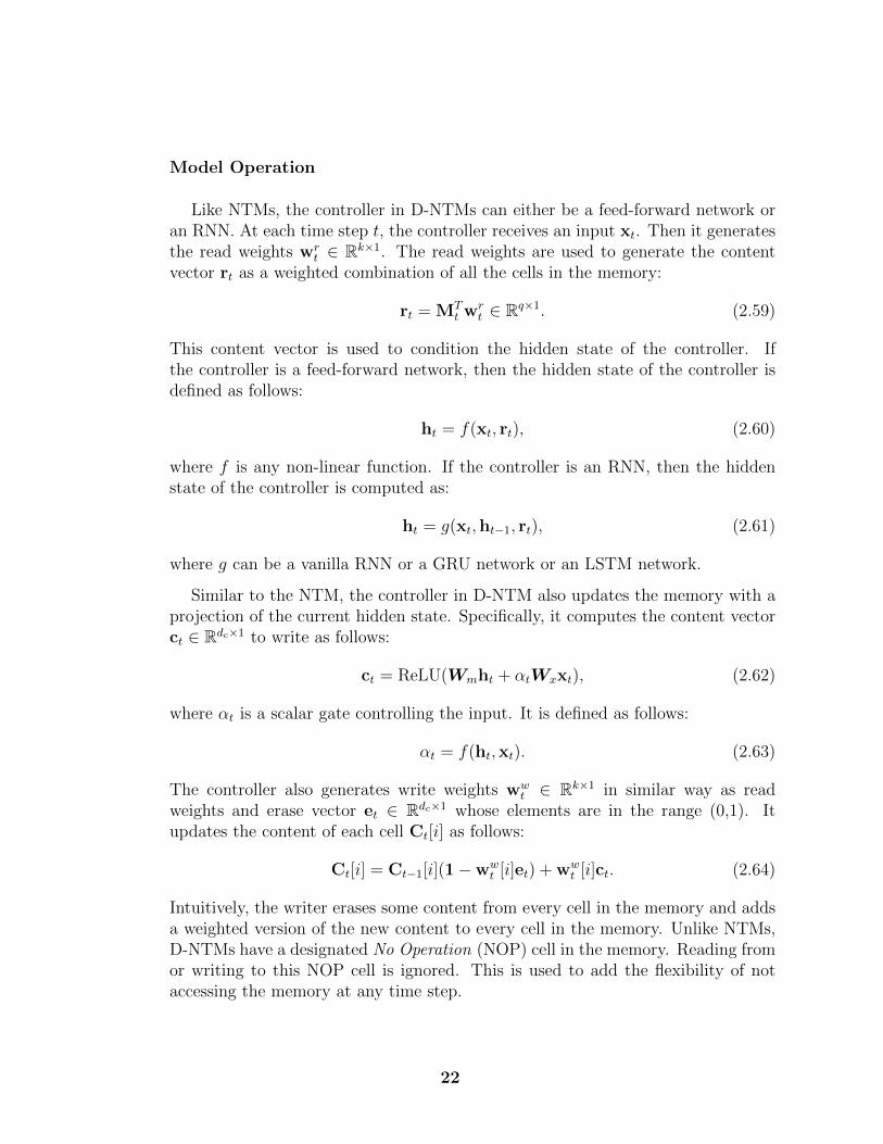
Model Operation

Like NTMs, the controller in D-NTMs can either be a feed-forward network oran RNN. At each time step t, the controller receives an input xt. Then it generatesthe read weights wr

t ∈ Rk×1. The read weights are used to generate the contentvector rt as a weighted combination of all the cells in the memory:

rt = MTt wr

t ∈ Rq×1. (2.59)

This content vector is used to condition the hidden state of the controller. Ifthe controller is a feed-forward network, then the hidden state of the controller isdefined as follows:

ht = f(xt, rt), (2.60)

where f is any non-linear function. If the controller is an RNN, then the hiddenstate of the controller is computed as:

ht = g(xt,ht−1, rt), (2.61)

where g can be a vanilla RNN or a GRU network or an LSTM network.

Similar to the NTM, the controller in D-NTM also updates the memory with aprojection of the current hidden state. Specifically, it computes the content vectorct ∈ Rdc×1 to write as follows:

ct = ReLU(Wmht + αtWxxt), (2.62)

where αt is a scalar gate controlling the input. It is defined as follows:

αt = f(ht,xt). (2.63)

The controller also generates write weights wwt ∈ Rk×1 in similar way as read

weights and erase vector et ∈ Rdc×1 whose elements are in the range (0,1). Itupdates the content of each cell Ct[i] as follows:

Ct[i] = Ct−1[i](1−wwt [i]et) + ww

t [i]ct. (2.64)

Intuitively, the writer erases some content from every cell in the memory and addsa weighted version of the new content to every cell in the memory. Unlike NTMs,D-NTMs have a designated No Operation (NOP) cell in the memory. Reading fromor writing to this NOP cell is ignored. This is used to add the flexibility of notaccessing the memory at any time step.

22

Addressing Mechanism

We describe the addressing mechanism for the read head here. But the samedescription holds for the write heads as well.

The read head first generates a key for the memory access:

kt = f(xt,ht−1) ∈ Rq×1. (2.65)

The key is compared with each cell in the memory Mt by using some similaritymeasure S to generate the logits for the address weights as follows:

zt[i] = βtS[kt,Mt[i]], (2.66)

where βt is a positive key strength vector that can amplify or attenuate the pre-cision of the focus. Up to this point, the addressing mechanism looks like thecontent-based addressing in the NTM. But note that the memory also has a loca-tion part and hence this adressing mechanism is a mix of content-based addressingand location-based addressing.

While writing, sometimes it is effective to put more emphasis on the least re-cently used (LRU) memory locations so that the information is not concentratedin only few memory cells. To implement this effect, D-NTM computes the movingaverage of the logits as follows:

vt = 0.1vt−1 + 0.9zt. (2.67)

This accumulated vt is rescaled by a scalar gate γt ∈ (0, 1) and subtracted fromthe current logits before applying the softmax operator. The final weight is givenas follows:

wrt = softmax(zt − γtvt−1). (2.68)

By setting γt to 0, the model can choose to use pure content-based addressing.This is known as dynamic LRU addressing since the model can dynamically decidewhether to use LRU addressing or not.

D-NTM uses single head with multi-step addressing similar to Sukhbaatar et al.(2015) instead of multiple heads used by the NTM.

Discrete Addressing

wrt in Equation 2.68 is a continuous vector and if used as such, the entire ar-

chitecture is differentiable. The D-NTM with continuous wrt vector is known as

23

continuous D-NTM.

Note that wrt is a valid probability distribution over k memory cells. Gulcehre

et al. (2016) also propose a discrete D-NTM which samples an index from thisprobability distribution. The discrete address wr

t is defined as follows:

wrt [k] = I(k = j) (2.69)

where j ∼ wrt and I is an indicator function. While we sample the index during

training, we can use argmax index during inference. This discrete addressing makesthe model non-differentiable and hence Gulcehre et al. (2016) used REINFORCE(Williams, 1992) to approximate the gradient. Training discrete D-NTMs was alsodifficult. Hence the authors suggested a curriculum based training where the modelstarts with continuous addressing and moves to discrete addressing over the periodof training. It was shown that D-NTMs performed better than NTMs in severaltasks.

2.10 Normalization methods

Normalization methods are used in deep neural networks to avoid vanishinggradients due to saturating activation functions. The basic idea is to normalizethe pre-activations of a layer such that the activation function in that layer doesnot saturate. Batch Normalization (Ioffe and Szegedy, 2015) normalized the pre-activation based on the batch-level statistics. Consider the pre-activation x over amini-batch B = {x1,x2, ...,xm} of m examples. We first compute the mini-batchmean and variance as follows:

µB =1

m

m∑i=1

xi (2.70)

σ2B =

1

m

m∑i=1

(xi − µB)2 (2.71)

Then, we compute the normalized pre-activation xi by using the mini-batch meanand variance.

xi =xi − µB√σ2B + ε

(2.72)

24

where ε is a small non-zero value added for numerical stability. The input to theactivation function yi is computed as follows:

yi = γxi + β (2.73)

where γ and β are the scaling and the shifting parameters respectively. Theseparameters are also learnt as part of training. Finally, the hidden layer activationsare computed as

h = f(BN(x)) (2.74)

where f is the activation function, x is the pre-activation, and BN is the batch-normalization operation such that BN(x) = y. Note that the scale and the shiftallows the network to cancel the effect of normalization if the task demands it.During testing, we will use a global mean and variance computed from training set.

Batch Normalization has been extended for recurrent neural networks in (Cooi-jmans et al., 2016; Laurent et al., 2016). However, to obtain the best performanceusing recurrent batch-normalization, one has to track independent normalizationstatistics for each time-step. During inference time, it is not clear how to handlesequences longer than the training sequences.

Ba et al. (2016) introduced Layer normalization as an alternative to the recurrentbatch normalization. The basic proposal by Ba et al. (2016) is to compute thenormalization statistics using the hidden units in the same layer instead of usingmini-batch of examples. Specifically, we compute

µl =1

H

H∑i=1

xi (2.75)

σ2l =

1

H

H∑i=1

(xi − µl)2 (2.76)

where H is the number of hidden units in the layer and xi is the pre-activation fori-th hidden unit. Now, we compute the normalized pre-activations as follows:

x =x− µl√σ2l + ε

(2.77)

Similar to the batch normalization, the normalized pre-activation is both scaledand shifted before applying the activation function.

The main advantage of layer normalization over batch normalization is we donot need to compute batch-level statistics. Hence, it is very easy to extend layernormalization to RNNs. We can apply layer normalization for pre-activations of

25

every activation function used in RNNs, LSTMs, or any other recurrent architec-tures. Ba et al. (2016) report that layer normalization helps in faster convergenceand also achieves better performance for several recurrent architectures.

26

3 LSTMs with WormholeConnections

In this chapter, we propose our first solution to avoid vanishing gradients calledTARDIS (Gulcehre et al., 2017).

3.1 Introduction

Memory augmented neural networks (MANNs) such as neural Turing machine(NTM) (Graves et al., 2014; Rae et al., 2016), dynamic NTM (D-NTM) (Gulcehreet al., 2016), and Differentiable Neural Computer (DNC) (Graves et al., 2016) usean external memory (usually a matrix) to store information and the MANN’s con-troller can learn to both read from and write into the external memory. As weshow here, it is in general possible to use particular MANNs to explicitly store theprevious hidden states of an RNN in the memory and that will provide shortcutconnections through time, called here wormhole connections, to look into thehistory of the states of the RNN controller. Learning to read and write into anexternal memory by using neural networks gives the model more freedom or flexi-bility to retrieve information from its past, forget or store new information into thememory. However, if the addressing mechanism for read and/or write operationsare continuous (like in the NTM and continuous D-NTM), then the access maybe too diffuse, especially early on during training. This can hurt especially thewriting operation, since a diffused write operation will overwrite a large fraction ofthe memory at each step, yielding fast vanishing of the memories (and gradients).On the other hand, discrete addressing, as used in the discrete D-NTM, should beable to perform this search through the past, but prevents us from using straightbackpropagation for learning how to choose the address.

We investigate the flow of the gradients and how the wormhole connections intro-duced by the controller affects it. Our results show that the wormhole connectionscreated by the controller of the MANN can significantly reduce the effects of thevanishing gradients by shortening the paths that the signal needs to travel betweenthe dependencies. We also discuss how the MANNs can generalize to sequenceslonger than the ones seen during the training.

27

In a discrete D-NTM, the controller must learn to read from and write into theexternal memory by itself and additionally, it should also learn the reader/writersynchronization. This can make learning more challenging. In spite of this diffi-culty, Gulcehre et al. (2016) reported that the discrete D-NTM can learn fasterthan the continuous D-NTM on some of the bAbI tasks. We provide a formalanalysis of gradient flow in MANNs based on discrete addressing and justify thisresult. In this chapter, we also propose a new MANN based on discrete address-ing called TARDIS (Temporal Automatic Relation Discovery in Sequences). InTARDIS, memory access is based on tying the write and read heads of the modelafter memory is filled up. When the memory is not full, the write head storesinformation in memory in the sequential order.

The main characteristics of TARDIS are as follows, TARDIS is a simple mem-ory augmented neural network model which can represent long-term dependenciesefficiently by using an external memory of small size. TARDIS represents thedependencies between the hidden states inside the memory. We show both the-oretically and experimentally that TARDIS fixes to a large extent the problemsrelated to long-term dependencies. Our model can also store sub-sequences or se-quence chunks into the memory. As a consequence, the controller can learn torepresent the high-level temporal abstractions as well. TARDIS performs well onseveral structured output prediction tasks as verified in our experiments.

The idea of using external memory with attention can be justified with theconcept of mental-time travel which humans do occasionally to solve daily tasks.In particular, in the cognitive science literature, the concept of chronesthesia isknown to be a form of consciousness which allows human to think about timesubjectively and perform mental time-travel (Tulving, 2002). TARDIS is inspiredby this ability of humans which allows one to look up past memories and plan forthe future using the episodic memory.

3.2 TARDIS: A Memory Augmented Neural

Network

Neural network architectures with an external memory represent the memoryin a matrix form, such that at each time step t the model can both read from andwrite to the external memory. The whole content of the external memory can beconsidered as a generalization of hidden state vector in a recurrent neural network.Instead of storing all the information into a single hidden state vector, our modelcan store them in a matrix which has a higher capacity and with more targetedability to substantially change or use only a small subset of the memory at each

28

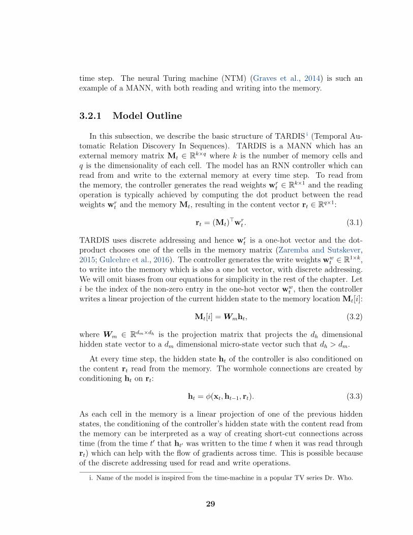
time step. The neural Turing machine (NTM) (Graves et al., 2014) is such anexample of a MANN, with both reading and writing into the memory.

3.2.1 Model Outline

In this subsection, we describe the basic structure of TARDIS i (Temporal Au-tomatic Relation Discovery In Sequences). TARDIS is a MANN which has anexternal memory matrix Mt ∈ Rk×q where k is the number of memory cells andq is the dimensionality of each cell. The model has an RNN controller which canread from and write to the external memory at every time step. To read fromthe memory, the controller generates the read weights wr

t ∈ Rk×1 and the readingoperation is typically achieved by computing the dot product between the readweights wr

t and the memory Mt, resulting in the content vector rt ∈ Rq×1:

rt = (Mt)>wr

t . (3.1)

TARDIS uses discrete addressing and hence wrt is a one-hot vector and the dot-

product chooses one of the cells in the memory matrix (Zaremba and Sutskever,2015; Gulcehre et al., 2016). The controller generates the write weights ww

t ∈ R1×k,to write into the memory which is also a one hot vector, with discrete addressing.We will omit biases from our equations for simplicity in the rest of the chapter. Leti be the index of the non-zero entry in the one-hot vector ww

t , then the controllerwrites a linear projection of the current hidden state to the memory location Mt[i]:

Mt[i] = Wmht, (3.2)

where Wm ∈ Rdm×dh is the projection matrix that projects the dh dimensionalhidden state vector to a dm dimensional micro-state vector such that dh > dm.

At every time step, the hidden state ht of the controller is also conditioned onthe content rt read from the memory. The wormhole connections are created byconditioning ht on rt:

ht = φ(xt,ht−1, rt). (3.3)

As each cell in the memory is a linear projection of one of the previous hiddenstates, the conditioning of the controller’s hidden state with the content read fromthe memory can be interpreted as a way of creating short-cut connections acrosstime (from the time t′ that ht′ was written to the time t when it was read throughrt) which can help with the flow of gradients across time. This is possible becauseof the discrete addressing used for read and write operations.

i. Name of the model is inspired from the time-machine in a popular TV series Dr. Who.

29

However, the main challenge for the model is to learn proper read and writemechanisms so that it can write the hidden states of the previous time steps thatwill be useful for future predictions and read them at the right time step. We callthis the reader/writer synchronization problem. Instead of designing complicatedaddressing mechanisms to mitigate the difficulty of learning how to properly ad-dress the external memory, TARDIS side-steps the reader/writer synchronizationproblem by using the following heuristics. For the first k time steps, our modelwrites the micro-states into the k cells of the memory in a sequential order. Whenthe memory becomes full, the most effective strategy in terms of preserving theinformation stored in the memory would be to replace the memory cell that hasbeen read with the micro-state generated from the hidden state of the controllerafter it is conditioned on the memory cell that has been read. If the model needsto perfectly retain the memory cell that it has just overwritten, the controller canin principle learn to do that by copying its read input to its write output (intothe same memory cell). The pseudocode and the details of the memory updatealgorithm for TARDIS is presented in Algorithm 1.

Algorithm 1 Pseudocode for the controller and memory update mechanism ofTARDIS.

1: Initialize h0

2: Initialize M0

3: for t ∈ {1, · · ·Tx} do4: Compute the read weights wr

t ← read(ht,Mt,xt)5: Sample from/discretize wr

t and obtain wrt

6: Read from the memory, rt ← (Mt)>wr

t .7: Compute a new controller hidden state, ht ← φ(xt,ht−1, rt)8: if t ≤ k then9: Write into the memory, Mt[t]←Wmht

10: else11: Select the memory location to write into j ← argmaxj(w

rt [j])

12: Write into the memory, Mt[j]←Wmht

There are two missing pieces in Algorithm 1: How to generate the read weights?What is the structure of the controller function φ? We will answer these twoquestions in detail in next two sub-sections.

3.2.2 Addressing mechanism

Similar to the D-NTM, memory matrix Mt of TARDIS has disjoint addresssection At ∈ Rk×a and content section Ct ∈ Rk×c, Mt = [At; Ct] and Mt ∈ Rk×q

for q = c+ a. However, unlike in the D-NTM, address vectors are fixed to random

30

sparse vectors. The controller reads both the address and the content parts of thememory, but it will only write into the content section of the memory.

The continuous read weights wrt are generated by an MLP which uses the in-

formation coming from ht, xt, Mt and the usage vector ut (described below). TheMLP is parametrized as follows:

πt[i] = a>tanh(W γh ht +W γ

x xt +W γmMt[i] +W γ

u ut) (3.4)

wrt = softmax(πt), (3.5)

where {a,W γh ,W

γx ,W

γm,W

γu } are learnable parameters. wr

t is a one-hot vectorobtained by either sampling from wr

t or by using argmax over wrt .

ut is the usage vector which denotes the frequency of accesses to each cell inthe memory. ut is computed from the sum of discrete address vectors wr

t andnormalizing them:

ut = norm(t−1∑i=1

wri ). (3.6)

The norm(·) applied in Equation 3.6 is a simple feature-wise computation of center-ing and divisive variance normalization. This normalization step makes the trainingeasier with the usage vectors. The introduction of the usage vector can help theattention mechanism to choose between the different memory cells based on theirfrequency of accesses to each cell of the memory. For example, if a memory cell isvery rarely accessed by the controller, for the next time step, it can learn to assignmore weights to those memory cells by looking into the usage vector. This way,the controller can learn an LRU access mechanism (Santoro et al., 2016; Gulcehreet al., 2016).

Further, in order to prevent the model to learn deficient addressing mechanisms,for e.g. reading the same memory cell which will not increase the memory capacityof the model, we decrease the probability of the last read memory location bysubtracting 100 from the logit of wr

t for that particular memory location.

3.2.3 TARDIS Controller

We use an LSTM controller, and its gates are modified to take into account thecontent rt of the cell read from the memory: ft

itot

=

sigm

sigm

sigm

(Whht−1 + Wxxt + Wrrt) , (3.7)

31

where ft, it, and ot are the forget gate, input gate, and output gate respectively.

The cell of the LSTM controller, ct is computed according to the Equation 3.8as follows:

ct = tanh(αtWhht−1 +W

xxt + βtWrrt),

ct = ftct−1 + itct, (3.8)

where αt, βt are the scalar RESET gates which control the magnitude of the in-formation flowing from the memory and the previous hidden states to the cell ofthe LSTM ct. By controlling the flow of information into the LSTM cell, thosegates will allow the model to store the sub-sequences or chunks of sequences intothe memory instead of the entire context.

We use Gumbel sigmoid (Maddison et al., 2016; Jang et al., 2016) for αt and βtdue to its behavior close to binary:(

αtβt

)=

(gumbel-sigmoidgumbel-sigmoid

)((wα>h

wβ>h

)ht−1 +

(wα>x

wβ>x

)xt +

(wα>r

wβ>r

)rt

), (3.9)

We find Gumbel-sigmoid to be easier to train than the regular sigmoid. Thetemperature of the Gumbel-sigmoid is fixed to 0.3 in all our experiments.

The hidden state of the LSTM controller is computed as follows:

ht = ot tanh(ct). (3.10)

In Figure 3.1, we illustrate the interaction between the controller and the mem-ory with various heads and components of the controller.

3.2.4 Micro-states and Long-term Dependencies

A micro-state of the LSTM for a particular time step is the summary of theinformation that has been stored in the LSTM controller of the model. By attendingover the cells of the memory which contains previous micro-states of the LSTM,the model can explicitly learn to restore information from its past.

The controller can learn to represent high-level temporal abstractions by cre-ating wormhole connections through the memory as illustrated in Figure 3.2. Inthis example, the model takes the token x0 at the first time-step and stores itsrepresentation to the first memory cell with address a0. In the second time-step,the controller takes x1 as input and writes into the second memory cell with theaddress a1. Furthermore, the β1 gate blocks the connection from h1 to h2. At the

32

a0

a1

a2

m0

m1

m2

Mt-1

ht⍺t

ct

xt

yt

mt

a0

a1

a2

m0

m1

m2

Mt

rtLegend:

: MLP output

: Read/Write output

: Observed Input

: Output prediction

: General Connection

: Multiplicative Connection

: Affine Connection

: Controller

Figure 3.1 – At each time step, controller takes xt, the memory cell that has been read rtand the hidden state of the previous timestep ht−1. Then, it generates αt which controls thecontribution of the rt into the internal dynamics of the new controller’s state ht (We omit theβt in this visualization). Once the memory Mt becomes full, discrete addressing weights wr

t isgenerated by the controller which will be used to both read from and write into the memory. Topredict the target yt, the model will have to use both ht and rt.

33

x0 x1 x2 x3 x4 x5

h0

h0

Write h0 to a0

x0

a0a1

Dependencies among the input tokens:

M0h0

h1

Write h1 to a1

x1

a0a1

M1h1

h0

h2

Write h2 to a0

x2

a0a1

M2

h1

h0

h3

Write h3 to a1

x3

a0a1

M3h1

h0

h4

Write h4 to a0

x4

a0a1

M4h1

h2 h2h3

h0

h5

Write h5 to a1

x5

a0a1

M5h1

h2 h4h3

h2 h4h3 h5

Read a0

β0=1 β1=0 β2=1 β3=0 β4=0

Read a1 Read a0 Read a1

Figure 3.2 – TARDIS’s controller can learn to represent the dependencies among the inputtokens by choosing which cells to read and write and creating wormhole connections. xt representsthe input to the controller at timestep t and the ht is the hidden state of the controller RNN.

third time-step, the controller starts reading. It receives x2 as input and reads thefirst memory cell where micro-state of h0 was stored. After reading, it computesthe hidden-state h2 and writes the micro-state of h2 into the first memory cell. Thelength of the path passing through the micro-states of h0 and h2 would be 1. Thewormhole connection from h2 to h0 would skip a time-step.

A regular single-layer RNN has a fixed graphical representation of a linear-chainwhen considering only the connections through its recurrent states or the temporalaxis. However, TARDIS is more flexible in that it can learn directed graphs withmore diverse structures using the wormhole connections and the RESET gates.The directed graph that TARDIS can learn through its recurrent states have atmost a degree of 4 at each vertex (maximum 2 incoming and 2 outgoing edges) andit depends on the number of cells (k) that can be stored in the memory.

In this work, we focus on a variation of TARDIS, where the controller maintainsa fixed-size external memory. However as in (Cheng et al., 2016), it is possible touse a memory that grows with respect to the length of its input sequences, butthat would not scale and can be more difficult to train with discrete addressing.

3.3 Training TARDIS

In this section, we explain how to train TARDIS as a language model. We uselanguage modeling as an example application. However, we would like to highlight

34

that TARDIS can also be applied to any complex sequence to sequence learningtask.

Consider N training examples where each example is a sequence of length T .At every time-step t, the model receives the input xt ∈ {0, 1}|V | which is a one-hot vector of size equal to the size of the vocabulary |V | and should produce theoutput yt ∈ {0, 1}|V | which is also a one-hot vector of size equal to the size of thevocabulary |V |.

The output of the model for the i-th example and t-th time-step is computed asfollows:

oit = softmax(W og(h(i)t , r

(i)t )), (3.11)

where W o are the learnable parameters and g(ht, rt) is a single layer MLP whichcombines both ht and rt as in deep fusion by Pascanu et al. (2013a). The taskloss would be the categorical cross-entropy between the targets and model outputs.Superscript i denotes that the variable is the output for the ith sample in thetraining set.

Lmodel(θ) = − 1

N

N∑i=1

T∑t=1

|V |∑k=1

y(i)t [k] log(o

(i)t [k]), (3.12)

However, the discrete decisions taken for memory access during every time-stepmakes the model not differentiable and hence we need to rely on approximatemethods of computing gradients with respect to the discrete address vectors. Inthis work we explore two such approaches: REINFORCE (Williams, 1992) and thestraight-through estimator (Bengio et al., 2013).

3.3.1 Using REINFORCE

REINFORCE is a likelihood-ratio method, which provides a convenient andsimple way of estimating the gradients of the stochastic actions. In this work,we focus on application of REINFORCE on sequential prediction tasks, such aslanguage modelling. For example i, let R(w

r(i)j ) be the reward for the action w

r(i)j

at timestep j. We are interested in maximizing the expected return for the wholeepisode as defined below:

J (θ) = E[T∑j=0

R(wr(i)j )] (3.13)

35

Ideally we would like to compute the gradients for Equation 3.13, however com-puting the gradient of the expectation may not be feasible. We would have to usea Monte-Carlo approximation and compute the gradients by using REINFORCEfor the sequential prediction task which can be written as in Equation 3.14.

∇θJ (θ) =1

N

N∑i=1

[T∑j=0

(R(wr(i)j )− bj)

T∑t=0

∇θ log(wr(i)t )], (3.14)

where bj is the reward baseline. However, we can further assume that the futureactions do not depend on the past rewards in the episode/trajectory and furtherreduce the variance of REINFORCE as in Equation 3.15.

∇θJ (θ) =1

N

N∑i=1

[T∑t=0

T∑j=t

(R(wr(i)j )− bj)∇θ log(w

r(i)t )], (3.15)

In our preliminary experiments, we find that the training of the model is easierwith discounted returns, instead of using the centered undiscounted return:

∇θJ (θ) =1

N

N∑i=1

[T∑t=0

T∑j=t

[γj−t(R(wr(i)j )− bj)]∇θ log(w

r(i)t )]. (3.16)

REINFORCE Training with an Auxiliary Cost Training models with RE-INFORCE can be difficult, due to the variance imposed into the gradients. Inrecent years, researchers have developed several tricks in order to mitigate the ef-fect of high-variance in gradients. As proposed by (Mnih and Gregor, 2014), wealso use variance normalization on the REINFORCE gradients.

For TARDIS, reward at timestep j (R(wr(i)j )) is the log-likelihood of the predic-

tion at that timestep. Our initial experiments showed that REINFORCE with thisreward structure often tends to under-utilize the memory and mainly rely on theinternal memory of the LSTM controller. Especially, in the beginning of training,it can just decrease the loss by relying on the memory of the controller and thiscan cause REINFORCE to increase the log-likelihood of the random actions.

In order to deal with this issue, instead of using the log-likelihood of the model asreward, we introduce an auxiliary cost to use as the reward R′ which is computedbased on predictions which are only based on the memory cell rt read by thecontroller and not the hidden state of the controller:

R′(wr(i)j ) =

|V |∑k=1

y(i)j [k] log(softmax(W o

r r(i)j +W o

xx(i)j ))[k], (3.17)

36

In Equation 3.17, we only train the parameters {W or ∈ Rdo×dm ,W o

x ∈ Rdo×dx}where do is the dimensionality of the output size and dx (for language modellingboth do and dx would be do = |V |) is the dimensionality of the input of the model.

We do not backpropagate through r(j)i and thus we denote it as r

(j)i in our equations.

3.3.2 Using Gumbel Softmax

Training with REINFORCE can be challenging due to the high variance of thegradients. Gumbel-softmax provides a good alternative with its straight-throughestimator to tackle the variance issue. Unlike (Maddison et al., 2016; Jang et al.,2016) instead of annealing the temperature or fixing it, our model learns the inverse-temperature with an MLP τ(ht) which has a single scalar output conditioned onthe hidden state of the controller.

τ(ht) = softplus(wτ>ht + bτ ) + 1. (3.18)

gumbel-softmax(πt[i]) = softmax((πt[i] + ξ)τ(ht)), (3.19)

We replace the softmax in Equation 3.5 with gumbel-softmax defined above. Duringforward computation, we sample from wr

t and use the generated one-hot vector wrt

for memory access. However, during backprop, we use wrt for gradient computation

and hence the entire model becomes differentiable.

Learning the temperature of the Gumbel-Softmax reduces the burden of per-forming extensive hyper-parameter search for the temperature.

3.4 Gradient Flow through the External

Memory

In this section, we analyze the flow of the gradients through the external mem-ory and will also investigate its efficiency in terms of dealing with the vanishinggradients problem (Hochreiter, 1991; Bengio et al., 1994). In our analysis, we alsoassume that the weights for the read/write heads are discrete.

We will show that the rate of the gradients vanishing through time for a memory-augmented recurrent neural network is much smaller than of a regular vanilla re-current neural network.

Consider the MANN where the contents of the memory are linear projections ofthe previous hidden states as described in Equation 3.2. Let us assume that both

37

reading and writing operations use discrete addressing. Let the content read fromthe memory at time step t correspond to some memory location i:

rt = Mt[i] = Ahit , (3.20)

where hit corresponds to the hidden state of the controller at some previous timestepit.

Now the hidden state of the controller in the external memory model can bewritten as,

zt = Wht−1 + Vrt +Uxt,

ht = f(zt). (3.21)

If the controller reads Mt[i] at time step t and its memory content is Ahit asdescribed above, then the Jacobians associated with Equation 3.21 can be computedas follows:

∂ht1∂ht0

=∏

t0<t≤t1

∂ht∂ht−1

=

( ∏t0<t≤t1

diag[f′(zt)]W

)+

t1−1∑k=t0

(∏

k<t∗<t1

diag[f′(zt∗)]W ) diag[f′(zk)]VA∂hik∂ht0

+ diag[f′(zt1)]VA∂hit1∂ht0

(3.22)

= Qt1t0 + Rt1t0 . (3.23)

where Qt1t0 and Rt1t0 are defined as,

Qt1t0 =∏

t0<t≤t1

diag[f′(zt)]W , (3.24)

Rt1t0 =t−1∑k=t0

(∏

k<t∗<t


+ diag[f′(zt1)]VA∂hit1∂ht0

.

(3.25)

As shown in Equation 3.23, Jacobians of the MANN can be rewritten as asummation of two matrices, Qt1t0 and Rt1t0 . The gradients flowing through Rt1t0

do not necessarily vanish through time, because it is the sum of jacobians computedover the shorter paths.

The norm of the Jacobian can be lower bounded as follows by using the Minkowski

38

inequality:

||∂ht1∂ht0|| = ||

∏t0<t≤t1

∂ht∂ht−1

|| (3.26)

= ||Qt1t0 + Rt1t0|| ≥ ||Rt1t0|| − ||Qt1t0||. (3.27)

Assuming that the length of the dependency is very long ||Qt1t0|| would vanishto 0. Then we will have,

||Qt1t0 + Rt1t0|| ≥ ||Rt1t0||. (3.28)

The rate of the gradients vanishing through time depends on the length of thesequence passing through Rt1t0 . This is typically less than the length of the se-quence passing through Qt1t0 . Thus the gradients vanish at a smaller rate than inan RNN. In particular the rate would strictly depend on the length of the shortestpaths from t1 to t0, because for the long enough dependencies, gradients throughthe longer paths would still vanish.

We can also derive an upper bound for the norm of the Jacobian as follows:

||∂ht1∂ht0|| = ||

∏t0<t≤t1

∂ht∂ht−1

|| (3.29)

= ||Qt1t0 + Rt1t0|| ≤ σ1(Qt1t0 + Rt1t0) (3.30)

where σ1(M) is the largest singular value of matrix M. Using the result from(Loyka, 2015), we can lower bound σ1(Qt1t0 + Rt1t0) as follows:

σ1(Qt1t0 + Rt1t0) ≥ |σ1(Qt1t0)− σ1(Rt1t0)| (3.31)

For long sequences we know that σ1(Qt1t0) will go to 0 (see equation 2.16).Hence,

σ1(Qt1t0 + Rt1t0) ≥ σ1(Rt1t0) (3.32)

The rate at which σ1(Rt1t0) reaches zero is strictly smaller than the rate at whichσ1(Qt1t0) reaches zero and with ideal memory access, it will not reach zero. Henceunlike vanilla RNNs, Equation 3.32 states that the upper bound of the norm of theJacobian will not reach zero for a MANN with ideal memory access.

Theorem 1. Consider a memory augmented neural network with T memory cellsfor a sequence of length T , and each hidden state of the controller is stored in

39

different cells of the memory. If the prediction at time step t1 has only a long-termdependency to t0 and the prediction at t1 is independent from the tokens appearingbefore t0, and the memory reading mechanism is perfect, then the model will notsuffer from vanishing gradients when we back-propagate from t1 to t0. i

Proof: If the input sequence has a longest-dependency on t0 for t1, we wouldonly be interested in gradients propagating from t1 to t0 and the Jacobians fromt1 to t0, i.e.

∂ht1

∂ht0. If the controller learns a perfect reading mechanism at time step

t1 it would read memory cell where the hidden state of the RNN at time step t0is stored at. Thus following the Jacobians defined in the Equation 3.23, we canrewrite the Jacobians as,

∂ht1∂ht0

=∏

t0<t≤t1

∂ht∂ht−1

=

( ∏t0<t≤t1

diag[f′(zt)]W

)+

t1−1∑k=t0

(∏

k<t∗<t1


+ diag[f′(zt1)]VA∂ht0∂ht0

(3.33)

In Equation 3.33, the first two terms might vanish as t1 − t0 grows. However,the singular values of the third term do not change as t1 − t0 grows. As a result,the gradients propagated from t1 to t0 will not necessarily vanish through time.However, in order to obtain stable dynamics for the network, the initialization ofthe matrices, V and A is important. �

This analysis highlights the fact that an external memory model with optimalread/write mechanism can handle long-range dependencies much better than anRNN. However, this is applicable only when we use discrete addressing for read-/write operations. Both NTM and D-NTM still have to learn how to read and writefrom scratch which is a challenging optimization problem. For TARDIS, tying theread/write operations make the learning become much simpler for the model. Inparticular, the results of the Theorem 1 points the importance of coming up withbetter ways of designing attention mechanisms over the memory.

The controller of a MANN may not be able learn to use the memory efficiently.For example, some cells of the memory may remain empty or may never be read.The controller can overwrite the memory cells which have not been read. As a resultthe information stored in those overwritten memory cells can be lost completely.However TARDIS avoids most of these issues by the construction of the algorithm.

i. Let us note that, unlike the Markovian n-gram assumption, here we assume that at eachtime step the dependency length n can be different.

40

3.5 On the Length of the Paths Through the

Wormhole Connections

As we have discussed in Section 3.4, the rate at which the gradients vanish for aMANN depends on the length of the paths passing along the wormhole connections.In this section we will analyse those lengths in depth for untrained models suchthat the model will assign uniform probability to read or write all memory cells.This will give us a better idea on how each untrained model uses the memory atthe beginning of the training.

A wormhole connection can be created by reading a memory cell and writinginto the same cell in TARDIS. For example, in Figure 3.2, while the actual pathfrom h4 to h0 is of length 4, memory cell a0 creates a shorter path of length 2(h0 → h2 → h4). We call the length of the actual path T and the length of theshorter path created by wormhole connections Tmem.

Consider a TARDIS model which has k cells in its memory. If TARDIS accesseseach memory cell uniformly at random, then the probability of accessing a randomcell i, p[i] = 1

k. The expected length of the shorter path created by wormhole

connections (Tmem) would be proportional to the number of reads and writes intoa memory cell. For TARDIS with reader choosing a memory cell uniformly atrandom, this would be Tmem =

∑Ti=k p[i] = T

k− 1 at the end of the sequence. We

verify this result by simulating the read and write heads of TARDIS as in Figure3.3 (a).

0 50 100 150 200

Num timesteps

0

2

4

6

8

10

12

Expe

cted

leng

th o

f pat

hs th

roug

h w

orm

hole

con

nect

ions

memory size 25memory size 50

a)

0 50 100 150 200

Num timesteps

0

2

4

6

8

10

12

Expe

cted

leng

th o

f pat

hs th

roug

h w

orm

hole

con

nect

ions

memory size 25memory size 50

b)

Figure 3.3 – In these figures we visualized the expected path length in the memory cells for asequence of length 200, memory size 50 with 100 simulations. a) shows the results for TARDISand b) shows the simulation for uMANN with uniformly random read and write heads.

Now consider a MANN with separate read and write heads each accessing thememory in discrete and uniformly random fashion. Let us call it uMANN. We willcompute the expected length of the shorter path created by wormhole connections

41

(Tmem) for uMANN. wrt and ww

t are the read and write head weights, each sampledfrom a multinomial distribution with uniform probability for each memory cellsrespectively. Let jt be the index of the memory cell read at timestep t. For anymemory cell i, len(·), defined below, is a recursive function that computes the lengthof the path created by wormhole connections in that cell.

len(Mt[i], i, jt) =

{len(Mt−1[jt], i, jt) + 1 if ww

t [i] = 1len(Mt−1[i], i, jt) if ww

t [i] = 0(3.34)

It is possible to prove that Tmem =∑

t Ei,jt [len(Mt[i], i, jt)] will be T/k − 1 byinduction for every memory cell. However, the proof assumes that when t is lessthan or equal to k, the length of all paths stored in the memory len(Mt[i], i, jt)should be 0. We have run simulations to compute the expected path length in amemory cell of uMANN as in Figure 3.3 (b).

This analysis shows that while TARDIS with uniform read head maintains thesame expected length of the shorter path created by wormhole connections asuMANN, it completely avoids the reader/writer synchronization problem.

If k is large enough, Tmem << T should hold. In expectation, σ1(Rt1t0) will decayproportionally to Tmem whereas σ1(Qt1t0) will decay proportional i to T . With idealmemory access, the rate at which σ1(Rt1t0) reaches zero would be strictly smallerthan the rate at which σ1(Qt1t0) reaches zero. Hence, as per Equation 3.32, theupper bound of the norm of the Jacobian will vanish at a much smaller rate.However, this result assumes that the dependencies on which the prediction reliesare accessible through the memory cell which has been read by the controller.

t0t1t0+n

t1-m

…

Figure 3.4 – Assuming that the prediction at t1 depends on the t0, a wormhole connection canshorten the path by creating a connection from t1 −m to t0 + n. A wormhole connection maynot directly create a connection from t1 to t0, but it can create shorter paths which the gradientscan flow without vanishing. In this figure, we consider the case where a wormhole connection iscreated from t1−m to t0 +n. This connections skips all the tokens in between t1−m and t0 +n.

In the more general case, consider a MANN with k ≥ T . The writer just fillsin the memory cells in a sequential manner and the reader chooses a memory cell

i. Exponentially when the Equation 2.16 holds.

42

uniformly at random. Let us call this model urMANN. Let us assume that thereis a dependency between two time-steps t0 and t1 as shown in Figure 3.4. If t0 wastaken uniformly between 0 and t1− 1, then there is a probability 0.5 that the readaddress invoked at time t1 will be greater than or equal to t0 (proof by symmetry).In that case, the expected shortest path length through that wormhole connectionwould be (t1 − t0)/2, but this still would not scale well. If the reader is very welltrained, it could pick exactly t0 and the path length will be 1.

Let us consider all the paths of length less than or equal to k + 1 of the formin Figure 3.4. Also, let n ≤ k/2 and m ≤ k/2. Then, the shortest path from t0 tot1 now has length n + m + 1 ≤ k + 1, using a wormhole connection that connectsthe state at t0 + n with the state at t1 −m. There are O(k2) such paths that arerealized, but we leave the distribution of the length of that shortest path as anopen question. However, the probability of hitting a very short path (of length lessthan or equal to k + 1) increases exponentially with k. Let the probability of theread at t1 −m to hit the interval (t0, t0 + k/2) be p. Then the probability thatthe shorter paths over the last k reads hits that interval is 1 − (1 − p)k/2, wherep is on the order of k/t1. On the other hand, the probability of not hitting thatinterval approaches to 0 exponentially with k.

Figure 3.4 illustrates how wormhole connections can create shorter paths. InFigure 3.5 (b), we show that the expected length of the path travelled outside thewormhole connections obtained from the simulations decreases as the size of thememory decreases. In particular, for urMANN and TARDIS the trend is very closeto exponential. As shown in Figure 3.5 (a), this also influences the total length ofthe paths travelled from time-step 50 to 5 as well. Writing into the memory byusing weights sampled with uniform probability for all memory cells cannot use thememory as efficiently as other approaches that we compare to. In particular fixingthe writing mechanism seems to be useful.

Even if the reader does not manage to learn where to read, there are many ”shortpaths” which can considerably reduce the effect of vanishing gradients.

3.6 On Generalization over the Longer

Sequences

Graves et al. (2014) have observed that LSTMs did not generalize well on se-quences substantially longer than the ones seen during the training. On the otherhand, a MANN such as an NTM or a D-NTM has been shown to generalize tolonger sequences on a set of toy tasks.

43

5 10 15 20 25 30 35 40 45 50

Memory Sizes

0

3

6

9

12

15

18

Leng

th o

f the

sho

rtest

pat

hs

MANN Uniform ReadMANN Uniform Read&WriteTARDIS

a)

5 10 15 20 25 30 35 40 45 50

Memory Sizes

0

3

6

9

12

15

18

Leng

th o

f the

sho

rtest

pat

hs o

utsi

de w

orm

hole

s

MANN Uniform ReadMANN Uniform Read&WriteTARDIS

b)

Figure 3.5 – We have run simulations for TARDIS, MANN with uniform read and write mech-anisms (uMANN) and MANN with uniform read and write head is fixed with a heuristic (ur-MANN). In our simulations, we assume that there is a dependency from timestep 50 to 5. We run200 simulations for each one of them with different memory sizes for each model. In plot a) weshow the results for the expected length of the shortest path from timestep 50 to 5. In the plots,as the size of the memory gets larger for both models, the length of the shortest path decreasesdramatically. In plot b), we show the expected length of the shortest path travelled outside thewormhole connections with respect to different memory sizes. TARDIS seems to use the memorymore efficiently compared to other models in particular when the size of the memory is small bycreating shorter paths.

We believe that the main reason for why LSTMs typically do not generalizeto sequences longer than the ones that are seen during training is mainly becausethe hidden state of an LSTM network utilizes an unbounded history of the inputsequence and as a result, its parameters are optimized using the maximum likeli-hood criterion to fit the sequences with lengths specific to the training examples.However, an n-gram language model or an HMM does not suffer from this issue.In comparison, an n-gram LM would use an input context with a fixed window sizeand an HMM has the Markov property in its latent space. As argued below, weclaim that while being trained, a MANN can also learn the ability to generalizefor sequences with a longer length than the ones that appear in the training set bymodifying the contents of the memory and reading from it.

A regular RNN will minimize the negative log-likelihood objective function forthe targets yt by using the unbounded history represented by the hidden state of theRNN, and it will model the parametrized conditional distribution p(yt|ht;θ) for theprediction at time-step t, while a MANN would learn p(yt|ht, rt;θ). If we assumethat rt represents all the dependencies that yt depends on in the input sequence,we will have p(yt|ht, rt;θ) ≈ p(yt|rt,xt;θ) where rt represents the dependencies ina limited context window that only contains paths shorter than the sequences seenduring training. Due to this property, we claim that MANNs such as NTM, D-NTMor TARDIS can generalize to longer sequences more easily. In our experiments on

44

PennTreebank, we show that a TARDIS language model trained to maximize thelog-likelihood for p(yt|ht, rt;θ) yields very close results while making predictionseven while using p(yt|rt,xt;θ) instead of p(yt|ht, rt;θ) during testing. The factthat the best results on bAbI dataset obtained in (Gulcehre et al., 2016) is with afeedforward controller and similarly in (Graves et al., 2014) a feedforward controllerwas used to solve some of the toy tasks also confirms our hypothesis. As a result,what has been written into the memory and what has been read becomes veryimportant to be able to generalize to the longer sequences.

3.7 Experiments

3.7.1 Character-level Language Modeling on PTB

As a preliminary study on the performance of our model we consider character-level language modelling. We have evaluated our models on the Penn TreeBank (PTB)corpus (Marcus et al., 1993) based on the train, valid and test sets used in (Mikolovet al., 2012). On this task, we are using layer-normalization (Ba et al., 2016) andrecurrent dropout (Semeniuta et al., 2016) as those are also used by the SOTAresults on this task. Using layer-normalization and recurrent dropout improves theperformance significantly and reduces the effects of overfitting. We train our mod-els with Adam (Kingma and Ba, 2014) over sequences of length 150. We show ourresults in Table 3.1.

In addition to the regular char-LM experiments, in order to confirm our hy-pothesis regarding the ability of MANNs to generalize to longer sequences, we havetrained a language model which learns p(yt|ht, rt;θ) by using a softmax layer asdescribed in Equation 3.11 and tested the performance using p(yt|rt,xt;θ). As inTable 3.1, the model’s performance by using p(yt|ht, rt;θ) is 1.26 BPC, howeverby using p(yt|rt,xt;θ) it becomes 1.28 BPC. This gap is small enough to confirmour assumption that p(yt|ht, rt;θ) ≈ p(yt|rt,xt;θ).

3.7.2 Sequential Stroke Multi-digit MNIST task

In this subsection, we introduce a new pen-stroke based sequential multi-digitMNIST prediction task as a benchmark for long term dependency modelling. Wealso benchmark the performance of LSTM and TARDIS on this challenging task.

45

Model BPCCW-RNN (Koutnik et al., 2014) 1.46

HF-MRNN (Sutskever et al., 2011) 1.41ME n-gram (Mikolov et al., 2012) 1.37

BatchNorm LSTM (Cooijmans et al., 2016) 1.32Zoneout RNN (Krueger et al., 2016) 1.27LayerNorm LSTM (Ha et al., 2016) 1.27

LayerNorm HyperNetworks (Ha et al., 2016) 1.23LayerNorm HM-LSTM & Step Fn. & Slope Annealing(Chung et al., 2016) 1.24

Our LSTM + Layer Norm + Dropout 1.28TARDIS + REINFORCE + R 1.28

TARDIS + REINFORCE + Auxiliary Cost 1.28TARDIS + REINFORCE + Auxiliary Cost + R 1.26

TARDIS + Gumbel Softmax + ST + R 1.25

Table 3.1 – Character-level language modelling results on Penn TreeBank Dataset. TARDISwith Gumbel Softmax and straight-through (ST) estimator performs better than REINFORCEand it performs competitively compared to the SOTA on this task. ”+ R” notifies the use ofRESET gates α and β.

Task and Dataset

Recently (de Jong, 2016) introduced an MNIST pen stroke classification taskand also provided a dataset which consisted of pen stroke sequences representingthe skeleton of the digits in the MNIST dataset. Each MNIST digit image I isrepresented as a sequence of quadruples {dxi, dyi, eosi, eodi}Ti=1, where T is thenumber of pen strokes to define the digit, (dxi, dyi) denotes the pen offset from theprevious to the current stroke (can be 1, -1 or 0), eosi is a binary valued featureto denote end of stroke and eodi is another binary valued feature to denote endof the digit. In the original dataset, the first quadruple contains absolute values(x, y) instead of offsets (dx, dy). Without loss of generality, we set the startingposition (x, y) to (0, 0) in our experiments. Each digit is represented by 40 strokesin average and the task is to predict the digit at the end of the stroke sequence.

While this dataset was proposed for incremental sequence learning in (de Jong,2016), we consider the multi-digit version of this dataset to benchmark modelsthat can handle long term dependencies. Specifically, given a sequence of pen-stroke sequences, the task is to predict the sequence of digits corresponding to eachpen-stroke sequences in the given order. This is a challenging task since it requiresthe model to learn to predict the digit based on the pen-stroke sequence, countthe number of digits and remember them and generate them in the same orderafter seeing all the strokes. In our experiments we consider 3 versions of this task

46

with 5, 10, and 15 digit sequences respectively. We generated 200,000 training datapoints by randomly sampling digits from the training set of the MNIST dataset.Similarly we generated 20,000 validation and test data points by randomly sam-pling digits from the validation set and test set of the MNIST dataset respectively.Average length of the stroke sequences in each of these tasks are 199, 399, and 599respectively.

4 6 3 2

<bos> 4 6 3

Figure 3.6 – An illustration of the sequential MNIST strokes task with multiple digits. Thenetwork is first provided with the sequence of strokes information for each MNIST digits (locationinformation) as input, during the prediction the network tries to predict the MNIST digits thatit has just seen. When the model tries to predict, the predictions from the previous time stepsare fed back into the network. For the first time step, the model receives a special <bos> tokenwhich is fed into the model in the first time step when the prediction starts.

Results

We benchmark the performance of LSTM and TARDIS in this new task. Bothmodels receive the sequence of pen strokes and at the end of the sequence areexpected to generate the sequence of digits followed by a particular <bos> token.The tasks is illustrated in Figure 3.6. We evaluate the models based on per-digiterror rate. We also compare the performance of TARDIS with REINFORCE withthat of TARDIS with gumbel softmax. All the models were trained for the samenumber of updates with early stopping based on the per-digit error rate in thevalidation set. Results for all 3 versions of the task are reported in Table-3.2. Fromthe table, we can see that TARDIS performs better than the LSTM in all threeversions of the task. Also TARDIS with gumbel-softmax performs slightly betterthan TARDIS with REINFORCE, which is consistent with our other experiments.

We also compare the learning curves of all three models in Figure-3.7. From thefigure we can see that TARDIS learns to solve the task faster than the LSTM byeffectively utilizing the given memory slots. Also, TARDIS with gumbel softmaxconverges faster than TARDIS with REINFORCE.

47

Model 5-digits 10-digits 15-digits

LSTM 3.00% 3.54% 8.81%TARDIS with REINFORCE 2.09% 2.56% 3.67%TARDIS with gumbel softmax 1.89% 2.23% 3.09%

Table 3.2 – Per-digit based test error in sequential stroke multi-digit MNIST task with 5,10,and 15 digits.

0 5 10 15 20 25epochs

0.0

0.1

0.2

0.3

0.4

0.5

0.6

0.7

0.8

valid

atio

n er

ror r

ate

TARDIS+GumbelLSTMTARDIS+REINFORCE

5 digits

0 5 10 15 20 25 30 35epochs

0.0

0.1

0.2

0.3

0.4

0.5

0.6

0.7

0.8

0.9

valid

atio

n er

ror r

ate

TARDIS+GumbelTARDIS+REINFORCELSTM

10 digits

0 10 20 30 40 50 60 70 80epochs

0.0

0.1

0.2

0.3

0.4

0.5

0.6

0.7

0.8

0.9

valid

atio

n er

ror r

ate

LSTMTARDIS+REINFORCETARDIS+Gumbel

15 digits

Figure 3.7 – Learning curves for LSTM and TARDIS for sequential stroke multi-digit MNISTtask with 5, 10, and 15 digits respectively.

3.7.3 NTM Tasks

Graves et al. (2014) proposed associative recall and the copy tasks to evaluate amodel’s ability to learn simple algorithms and generalize to sequences longer thanthe ones seen during the training. We trained a TARDIS model with 4 featuresfor the address and 32 features for the memory content part of the model. Weused a model with hidden states of size 120. Our model uses a memory of size 16.We train our model with Adam and used a learning rate of 3e-3. We show theresults of our model in Table 3.3. TARDIS was able to solve both tasks, both withGumbel-softmax and REINFORCE.

48

Copy Task Associative Recall

D-NTM cont. (Gulcehre et al., 2016) Success SuccessD-NTM discrete (Gulcehre et al., 2016) Success FailureNTM (Graves et al., 2014) Success SuccessTARDIS + Gumbel Softmax + ST Success SuccessTARDIS REINFORCE + Auxiliary Cost Success Success

Table 3.3 – In this table, we consider a model to be successful on copy or associative recall if itsvalidation cost (binary cross-entropy) is lower than 0.02 over the sequences of maximum lengthseen during the training. We set the threshold to 0.02 to determine whether a model is successfulon a task as in (Gulcehre et al., 2016).

3.7.4 Stanford Natural Language Inference

Bowman et al. (2015) proposed a new task to test a machine learning algorithm’sability to infer whether two given sentences entail, contradict or are neutral (se-mantic independence) from each other. However, this task can be considered along-term dependency task if the premise and the hypothesis are presented to themodel in sequential order, as also explored by Rocktaschel et al. (2015). Becausethe model should learn the dependency relationship between the hypothesis andthe premise. Our model first reads the premise, then the hypothesis. At the end ofthe hypothesis, the model predicts whether the premise and the hypothesis contra-dicts or entails. The model proposed by Rocktaschel et al. (2015), applies attentionover its previous hidden states over the premise when it reads the hypothesis. Inthat sense their model can still be considered to have some task-specific architec-tural design choice. TARDIS and our baseline LSTM models do not include anytask-specific architectural design choices. In Table 3.4, we compare the results ofdifferent models. Our model performs better than the other models we compareagainst in this experiment. However recently it has been shown that with archi-tectural tweaks, it is possible to design a model specifically to solve this task andachieve 88.2% test accuracy (Chen et al., 2016).

3.8 Conclusion

In this chapter, we proposed a simple and efficient memory augmented neuralnetwork model which can perform well both on algorithmic tasks and more realistictasks. Unlike previous approaches, we show better performance on real-world NLPtasks, such as language modelling and SNLI. We have also proposed a new task tomeasure the performance of the models dealing with long-term dependencies.

49

Model Test AccuracyWord by Word Attention (Rocktaschel et al., 2015) 83.5

Word by Word Attention two-way (Rocktaschel et al., 2015) 83.2LSTM + LayerNorm + Dropout 81.7

TARDIS + REINFORCE + Auxiliary Cost 82.4TARDIS + Gumbel Softmax + ST 84.3

NTM 80.2D-NTM 80.9

LSTM (Bowman et al., 2015) 82.3NTM + Layer-Norm + Dropout 81.8

D-NTM + Layer-Norm + Dropout 82.3

Table 3.4 – Comparisons of different baselines on SNLI Task.

We provide a detailed analysis on the effects of using external memory for thegradients and justify the reason why MANNs generalize better on sequences longerthan the ones seen in the training set. We have also shown that the gradients willvanish at a much slower rate (if they vanish) when an external memory is beingused. Our theoretical results should encourage further studies in the directionof developing better attention mechanisms that can create wormhole connectionsefficiently.

50

4 Non-saturating RecurrentUnits

In this chapter, we introduce our second solution to mitigating vanishing gradi-ents, called Non-saturating Recurrent Units (NRUs) (Chandar et al., 2019).

4.1 Introduction

Successful architectures, like the LSTM (Hochreiter and Schmidhuber, 1997) andGRU (Cho et al., 2014), alleviate vanishing gradients by allowing information toskip transition operators (and their activation functions) via an additive path thatserves as memory. Both gates and transition operators use bounded activationfunctions (sigmoid, tanh). These help keep representations stable but attenuategradients in two ways: they are contractive and they saturate at the bounds. Acti-vation functions whose gradients contract as they saturate are typically referred toas saturating nonlinearities; in that sense, rectified linear units (ReLU) (Nair andHinton, 2010) are non-saturating and thus help reduce vanishing gradients in deepfeed-forward networks (Krizhevsky et al., 2012; Xu et al., 2015).

Saturating activation functions still dominate in the literature for recurrentneural networks, in part because of the success of LSTM on sequential problems(Sutskever et al., 2014; Vinyals and Le, 2015; Merity et al., 2017; Mnih et al., 2016).As these functions saturate, gradients contract. In addition, while saturated gatesmay push more information through memory and improve gradient flow across along sequence, the gradient to the gating units themselves vanishes. We expect thatnon-saturating activation functions and gates could improve the modelling of long-term dependencies by avoiding these issues. We propose a non-saturating recurrentunit (NRU) that forgoes both saturating activation functions and saturating gates.We present a new architecture with the rectified linear unit (ReLU) and demon-strate that it is well equipped to process data with long distance dependencies,without sacrificing performance on other tasks.

Saturating gating functions introduce a trade-off where distant gradient propa-gation may occur at the cost of vanishing updates to the gating mechanism. Weseek to avoid this trade-off between distant gradient propagation but not update-able gates (saturated gates) and short gradient propagation but updateable gates

51

(non-saturated gates). To that end, we propose the Non-saturating Recurrent Unit— a gated recurrent unit with no saturating activation functions.

4.2 Non-saturating Recurrent Units

At any time-step t, the NRU takes some input xt and updates its hidden stateas follows:

ht = f(Whht−1 +Wixt +Wcmt−1) (4.1)

where ht−1 ∈ Rh is the previous hidden state, mt−1 ∈ Rm is the previous memorycell, and f is a ReLU non-linearity. The memory cell in NRU is a flat vector similarto the cell vector in the LSTM. However, in NRU, the hidden state and the memorycell need not be of the same size. We allow the memory cell to be larger than thehidden state to hold more information.

At every time step t, memory cells are updated as follows:

mt = mt−1 +

k1∑i=1

αivwi −

k2∑i=1

βivei (4.2)

where— mt ∈ Rm is the memory vector at time t.— k1 is the number of writing heads and k2 is the number of erasing heads. We

often set k1 = k2 = k.— vwi ∈ Rm is a normalized vector which defines where to write in the memory.

Similarly vei ∈ Rm is a normalized vector which defines where to erase in thememory.

— αi is a scalar value which represents the content which is written in thememory along the direction of vwi . Similarly, βi is a scalar value whichrepresents the content which is removed from the memory along the directionof vei .

Intuitively, the network first computes a low-dimensional projection of the cur-rent hidden state by generating a k-dimensional α vector. Then it writes each unitof this k-dimensional vector along k different basis directions (vwi s). These k basisdirections specify where to write as continuous-valued vectors and hence there isno need for saturating non-linearities or discrete addressing schemes. The networkalso similarly erases some content from the memory (by using β and vei s).

52

Scalars αi and βi are computed as follows:

αi = fα(xt,ht,mt−1) (4.3)

βi = fβ(xt,ht,mt−1) (4.4)

where fα and fβ are linear functions followed by an optional ReLU non-linearity.Vectors vwi and vei are computed as follows:

vwi = fw(xt,ht,mt−1) (4.5)

vei = fe(xt,ht,mt−1) (4.6)

where fw and fe are linear functions followed by an optional ReLU non-linearityfollowed by an explicit normalization. We used L5 normalization in all of ourexperiments since it performed slightly better than L2 normalization in our initialexperiments.

Each v vector is m-dimensional and there are 2k such vectors that need to begenerated. This requires a lot of parameters which could create problems bothin terms of computational cost and in terms of overfitting. We reduce this largenumber of parameters by using the following outer product trick to factorize the vvectors:

pwi = fw1(xt,ht,mt−1) ∈ R√m (4.7)

qwi = fw2(xt,ht,mt−1) ∈ R√m (4.8)

vwi = g(vec(pwi qwiT )) (4.9)

where fw1 and fw2 are linear functions, vec() vectorizes a given matrix, g is anoptional ReLU non-linearity followed by an explicit normalization. Thus, insteadof producing an m-dimensional vector for the direction, we only need to produce a2√m-dimensional vector which requires substantially fewer parameters and scales

more reasonably. We can further reduce the number of parameters by generatinga 2√km-dimensional vector instead of 2k

√m-dimensional vector and then use the

outer product trick to generate the required km-dimensional vector. We do thistrick in our implementation of NRU.

If there is no final ReLU activation function while computing α, β, and v, thenthere is no distinction between write and erase heads. For example, either βi orvei could become negative, changing the erasing operation into one that adds tothe memory. Having an explicit ReLU activation in all these terms forces thearchitecture to use writing heads to add information to the memory and erasingheads to erase information from the memory. However, we treat this enforcementas optional and in some experiments, we let the network decide how to use theheads by removing these ReLU activations.

53

4.2.1 Discussion

In vanilla RNNs, the hidden state acts as the memory of the network. Sothere is always a contradiction between stability (which requires small enough Wh

to avoid explosions) and long-term storage (which requires high enough Wh toavoid vanishing gradients). This contradiction is exposed in a ReLU RNN whichavoids the saturation from gates at the cost of network stability. LSTM and GRUreduce this problem by introducing memory in the form of information skippedforward across transition operators, with gates determining which information isskipped. However, the gradient on the gating units themselves vanishes whenthe unit activations saturate. Since distant gradient propagation across memoryis aided by gates that are locked to ON (or OFF), this introduces an unfortunatetrade-off where either the gate mechanism receives updates or gradients are skippedacross many transition operators.

NRU also maintains a separate memory vector like the LSTM and GRU. Unlikethe LSTM and GRU, NRU does not have saturating gates. Even if the pathspurely through hidden states h vanish (with small enough Wh), the actual longterm memories are stored in memory vector m which has additive updates andhence no vanishing gradient.

Although the explicit normalization in vectors vwi and vei may cause gradientsaturation for large values, we focus on the nonlinearities because of their outsizedeffect on vanishing gradients. In comparison, the effect of normalization is lesspronounced than that of explicitly saturating nonlinearities like tanh or sigmoidwhich are also contractive based on our experiments. Also, normalization hasbeen employed to avoid the saturation regimes of these nonlinearities (Ioffe andSzegedy, 2015; Cooijmans et al., 2016). Furthermore, we observe that foregoingthese nonlinearities allows the NRU to converge much faster than other models.

4.3 Experiments

In this section, we compare the performance of NRU networks with severalother RNN architectures in three synthetic tasks (5 including variants) and tworeal tasks. Specifically, we consider the following extensive list of recurrent ar-chitectures: RNN with orthogonal initialization (RNN-orth), RNN with identityinitialization (RNN-id), LSTM (Hochreiter and Schmidhuber, 1997), LSTM withchrono initialization (LSTM-chrono) (Tallec and Ollivier, 2018), GRU (Cho et al.,2014), JANET (van der Westhuizen and Lasenby, 2018), SRU (Oliva et al., 2017),EURNN (Jing et al., 2017b), GORU (Jing et al., 2017a). We used the FFT-likealgorithm for the orthogonal transition operators in EURNN and GORU as it tends

54

to be much faster than the tunable algorithm, both proposed by Jing et al. (2017b).While these two algorithms have a low theoretical computational complexity, theyare difficult to parallelize.

We mention common design choices for all the experiments here: RNN-orth andRNN-id were highly unstable in all our experiments and we found that adding layernormalization helps. Hence all our RNN-orth and RNN-id experiments use layernormalization. We did not see any significant benefit in using layer normalizationfor other architectures and hence it is turned off by default for other architectures.NRU with linear writing and erasing heads performed better than with ReLU basedheads in all our experiments except the language model experiment. Hence we usedlinear writing and erasing heads unless otherwise mentioned. We used the Adamoptimizer (Kingma and Ba, 2014) with a default learning rate of 0.001 in all ourexperiments. We clipped the gradients by norm value of 1 for all models exceptGORU and EURNN since their transition operators do not expand norm. We useda batch size of 10 for most tasks, unless otherwise stated.

Table-4.1 summarizes the results of this section. Out of 10 different architecturesthat we considered, NRU is the only model that performs among the top 2 modelsacross all 7 tasks. The code for the NRU Cell is available at https://github.

com/apsarath/NRU.

Model in Top-1 in Top-2

RNN-orth 1 1RNN-id 1 1LSTM 1 1LSTM-chrono 1 1GRU 1 2JANET 1 3SRU 1 1EURNN 2 3GORU 0 1NRU 4 7

Table 4.1 – Number of tasks where the models are in top-1 and top-2. Maximum of 7 tasks.Note that there are ties between models for some tasks so the column for top-1 performance wouldnot sum up to 7.

4.3.1 Copying Memory Task

The copying memory task was introduced in Hochreiter and Schmidhuber (1997)as a synthetic task to test the network’s ability to remember information over manytime-steps. The task is defined as follows. Consider n different symbols. In the

55

https://github.com/apsarath/NRU

https://github.com/apsarath/NRU

0 25K 50K 75K 100K 125K 150K 175K 200KNumber of updates

0.00

0.05

0.10

0.15

0.20

0.25

0.30

Cross E

ntropy

Copying Memory Task, delay time T = 100LSTM-chronoNRUJANETGRURNN-orthRNN-idLSTMSRUEURNNGORU


0.00

0.05

0.10

0.15

0.20

0.25

0.30

Cross E

ntropy

Copying Memory Task, delay time T = 200LSTM-chronoNRUJANETGRURNN-orthRNN-idLSTMSRUEURNNGORU

Figure 4.1 – Copying memory task for T = 100 (in top) and T = 200 (in bottom). Cross-entropyfor random baseline : 0.17 and 0.09 for T=100 and T=200 respectively.

56

first k time-steps, the network receives an initial sequence of k random symbolsfrom the set of n symbols sampled with replacement. Then the network receivesa “blank” symbol for T − 1 steps followed by a “start recall” marker. The networkshould learn to predict a “blank” symbol, followed by the initial sequence after themarker. Following Arjovsky et al. (2016), we set n = 8 and k = 10. The copyingtask is a pathologically difficult long-term dependency task where the output atthe end of the sequence depends on the beginning of the sequence. We can vary thedependency length by varying the length of the sequence T . A memoryless modelis expected to achieve a sub-optimal solution which predicts a constant sequenceafter the marker, for any input (referred to as the “baseline” performance). Thecross-entropy for such a model would be klogn

T+2n(Arjovsky et al., 2016).

We trained all models with approximately the same number of parameters(∼23.5k), in an online fashion where every mini-batch is dynamically generated.We consider T = 100 and T = 200. In Figure 4.1 we plot the cross-entropy loss forall the models. Unsurprisingly, EURNN solves the task in a few hundred updatesas it is close to an optimal architecture tuned for this task (Henaff et al., 2016).Conversely, RNN-orth and RNN-id get stuck at baseline performance. NRU con-verges faster than all other models, followed by JANET which requires two to threetimes more updates to solve the task.

We observed the change in the memory vector across the time steps in Figure-4.2. We can see that the network has learnt to add information into the memoryin the beginning of the sequence and then it does not access the memory until itsees the marker. Then it makes changes in the memory in the last 10 time steps tocopy the sequence. Note that NRU has to make changes in the memory even whilecopying the sequence since there is no location based addressing of the memory.

We performed additional experiments following the observation by Henaff et al.(2016) that gated models like the LSTM outperform a simple non-gated orthogonalnetwork (similar to the EURNN) when the time lag T is varied in the copying task.This variable length task highlights the non-generality of the solution learned bymodels like EURNN. Only models with a dynamic gating mechanism can solvethis problem. In Figure-4.3, we plot the cross-entropy loss for all the models. Theproposed NRU model is the fastest to solve this task, followed by JANET, whilethe EURNN performs poorly, as expected according to Henaff et al. (2016). Thesetwo experiments highlight the fact that NRU can store information longer thanother recurrent architectures. Unlike EURNN which behaves like a fixed clockmechanism, NRU learns a gating function to lock the information in the memoryas long as needed. This is similar to the behaviour of other gated architectures.However, NRU beats other gated architectures mainly due to better gradient flowwhich results in faster learning. Figure-4.4 shows that NRU converges significantlyfaster than its strongest competitors (JANET and LSTM-chrono) in all the 4 tasks.

57

Figure 4.2 – Change in the content of the NRU memory vector for the copying memory taskwith T=100. We see that the network has learnt to use the memory in the first 10 time steps tostore the sequence. Then it does not access the memory until it sees the marker. Then it startsaccessing the memory to generate the sequence.

58


0.0

0.1

0.2

0.3

0.4

0.5

Cros

s Ent

ropy

Variable Copying Memory Task, delay time T = 1 to 100LSTM-chronoNRUJANETGRURNN-orthRNN-idLSTMSRUEURNNGORU


0.0

0.1

0.2

0.3

0.4

0.5

Cros

s Ent

ropy

Variable Copying Memory Task, delay time T = 1 to 200LSTM-chronoNRUJANETGRURNN-orthRNN-idLSTMSRUEURNNGORU

Figure 4.3 – Variable Copying memory task for T = 100 (in left) and T = 200 (in right).

59

Figure 4.4 – Comparison of top-3 models w.r.t the number of the steps to converge for differenttasks. NRU converges significantly faster than JANET and LSTM-chrono.

4.3.2 Denoising Task

The denoising task was introduced by Jing et al. (2017a) to test both the memo-rization and forgetting ability of RNN architectures. This is similar to the copyingmemory task. However, the data points are located randomly in a long noisy se-quence. Consider again an alphabet of n different symbols from which k randomsymbols are sampled with replacement. These symbols are then separated by ran-dom lengths of strings composed of a “noise” symbol, in a sequence of total lengthT . The network is tasked with predicting the k symbols upon encountering a “startrecall” marker, after the length T input sequence. Again we set n = 8 and k = 10.This task requires both an ability to learn long term dependencies and also anability to filter out unwanted information (considered noise).

The experimental procedure is exactly the same as described for the copyingmemory task. In Figure 4.5 we plot the cross-entropy loss for all the models forT = 100. In this task, all the models converge to the solution except EURNN. WhileNRU learns faster in the beginning, all the algorithms converge after approximatelythe same number of updates.

60


0.0

0.1

0.2

0.3

0.4

0.5

Cros

s Ent

ropy

Denoising Task, delay time T = 100LSTM-chronoJANETGRURNN-orthRNN-idLSTMSRUEURNNGORUNRU

Figure 4.5 – Denoising task for T = 100.

4.3.3 Character Level Language Modelling

Going beyond synthetic data, we consider character level language modellingwith the Penn Treebank Corpus (PTB) (Marcus et al., 1993). In this task, thenetwork is fed one character per time step and the goal is to predict the nextcharacter. Again we made sure that all the networks have approximately the samecapacity (∼2.15M parameters). We use a batch size of 128 and perform truncatedbackpropagation through time, every 150 time steps. We evaluate according to bitsper character (BPC) and accuracy.

All models were trained for 20 epochs and evaluated on the test set after selectingfor each the model state which yields the lowest BPC on the validation set. Thetest set BPC and accuracy are reported in Table-4.2. We did not add drop-out orbatch normalization to any model. From the table, we can see that GRU is thebest performing model, followed closely by NRU. We note that language modellingdoes not require very long term dependencies. This is supported by the fact thatchanging the additive memory updates in NRU to multiplicative updates doesnot hurt performance (it actually improves it). This is further supported by ourobservation that setting Tmax to 50 was better than setting Tmax to 150 in chrono-initialization for LSTM and JANET. All the best performing NRU models usedReLU activations in the writing and erasing heads.

61

Model BPC Accuracy

LSTM 1.48 67.98LSTM-chrono 1.51 67.41GRU 1.45 69.07JANET 1.48 68.50GORU 1.53 67.60EURNN 1.77 63.00NRU 1.47 68.48

Table 4.2 – Bits Per Character (BPC) and Accuracy in test set for character level languagemodelling in PTB.

4.3.4 Permuted Sequential MNIST

The Permuted Sequential MNIST task was introduced by Le et al. (2015) as abenchmark task to measure the performance of RNNs in modelling complex longterm dependencies. In a sequential MNIST task, all the 784 pixels of an MNISTdigit are fed to the network one pixel at a time and the network must classifythe digit in the 785th time step. Permuted sequential MNIST (psMNIST) makesthe problem harder by applying a fixed permutation to the pixel sequence, thusintroducing longer term dependencies between pixels in a more complex order.

For this task, we used a batch size of 100. All the networks have approximatelythe same number of parameters (∼165k). This corresponds to 200 to 400 hiddenunits for most of the architectures. Since the FFT-style algorithm used with EU-RNN requires few parameters, we used a large 1024 unit hidden state still achievingfewer parameters (∼17k parameters) at maximum memory usage. We report vali-dation and test accuracy in Table-4.3 and plot the validation curves in Figure-4.6.On this task, NRU performs better than all the other architectures, followed bythe EURNN. The good performance of the EURNN could be attributed to itslarge hidden state, since it is trivial to store all 784 input values in 1024 hiddenunits. This model excels at preserving information, so performance is boundedby the classification performance of the output layer. While NRU remains stable,RNN-orth and RNN-id are not stable as seen from the learning curve. Surprisingly,LSTM-chrono is not performing better than regular LSTM.

4.3.5 Model Analysis

Stability: While we use gradient clipping to limit exploding gradients in NRU,we observed gradient spikes in some of our experiments. We suspect that the net-work recovers due to consistent gradient flow. To verify that the additive nature

62

Figure 4.6 – Validation curve for psMNIST task.

Model valid test

RNN-orth 88.70 89.26RNN-id 85.98 86.13LSTM 90.01 89.86LSTM-chrono 88.10 88.43GRU 92.16 92.39JANET 92.50 91.94SRU 92.79 92.49EURNN 94.60 94.50GORU 86.90 87.00NRU 95.46 95.38

Table 4.3 – Validation and test set accuracy for psMNIST task.

63

of the memory does not cause memory to explode for longer time steps, we per-formed a sanity check experiment where we trained the model on the copy task(with T=100, 200, and 500) with random labels and observed that training didnot diverge. We observed some instabilities with all the models when training withlonger time steps (T = 2000). With NRU, we observed that the model convergedfaster and was more stable with a higher memory size. For instance, our modelconverged almost twice as early when we increased the memory size from 64 to 144.

Forgetting Ability: We performed another sanity check experiment to gaugethe forgetting ability of our model. We trained it on the copy task but reset thememory only once every k= 2, 5, and 10 examples and observed that NRU learnedto reset the memory in the beginning of every example.

Gradient Flow: To give an overview of the gradient flow across different timesteps during training, we compared the total gradient norms in the copying memorytask for the top 3 models: NRU, JANET and LSTM-Chrono (Figure 4.7). We seethat the NRU’s gradient norm is considerably higher during the initial stages ofthe training while the other model’s gradient norms rise after about 25k steps.After 25k steps, the drop in the NRU gradient norm coincides with the model’sconvergence, as expected. We expect that this ease of gradient flow in NRU servesas an additional evidence that NRU can model long-term dependencies better thanother architectures.

Figure 4.7 – Gradient norm comparison with JANET and LSTM-chrono across the trainingsteps. We observe significantly higher gradient norms for NRU during the initial stages comparedto JANET or LSTM-chrono. As expected, NRU’s gradient norms decline after about 25k stepssince the model has converged.

64

Hyper-parameter Sensitivity Analysis

NRU has three major hyper-parameters: memory size (m), number of heads(k) and hidden state size (h). To understand the effect of these design choices, wevaried each hyper-paramteter by fixing other hyper-parameters for the psMNISTtask. The baseline model was m = 256, k = 4, h = 200. We varied k ∈ {1, 4, 9, 16},m ∈ {100, 256, 400}, and h ∈ {50, 100, 200, 300}. We trained all the models for afixed number of 40 epochs. Validation curves are plotted in Figure-4.8. It appearsthat increasing k is helpful, but yields diminishing returns above 4 or 9. For ahidden state size of 200, a larger memory size (like 400) makes the learning difficultin the beginning, though all the models converge to a similar solution. This maybe due to the increased number of parameters. On the other hand, for a memorysize of 256, small hidden states appear detrimental.

Figure 4.8 – Effect of varying the number of heads (left), memory size (middle), and hiddenstate size (right) in psMNIST task.

4.4 Conclusion

In this chapter, we introduce Non-saturating Recurrent Units (NRUs) for mod-elling long term dependencies in sequential problems. The gating mechanism inNRU is additive (like in LSTM and GRU) and non-saturating (unlike in LSTMand GRU). This results in better gradient flow for longer durations. We presentempirical evidence in support of non-saturating gates in the NRU with (1) im-proved performance on long term dependency tasks, (2) higher gradient norms,and (3) faster convergence when compared to baseline models. NRU was the bestperforming general purpose model in all of the long-term dependency tasks thatwe considered and is competitive with other gated architectures in short-term de-pendency tasks. This work opens the door to other potential non-saturating gatedrecurrent network architectures.

65

We would also like to apply NRU in several real world sequential problems innatural language processing and reinforcement learning where the LSTM is thedefault choice for recurrent computation.

66

5On Training RecurrentNeural Networks forLifelong Learning

In the last two chapters, we explored the problem of learning long-term de-pendencies that arises when training recurrent neural networks with very long se-quences. The focus was on single-task setting. In this chapter, we explore thechallenges that arise while training RNNs in a multi-task lifelong learning setting.The results reported in this chapter appears in (Sodhani et al., 2019).

5.1 Introduction

Lifelong machine learning considers systems that can learn many tasks (from oneor more domains) over a lifetime (Thrun, 1998; Silver et al., 2013). This has sev-eral names and manifestations in the literature: incremental learning (Solomonoff,1989), continual learning (Ring, 1997), explanation-based learning (Thrun, 1996,2012), never-ending learning (Carlson et al., 2010), etc. The underlying idea mo-tivating these efforts is the following: lifelong learning systems would be moreeffective at learning and retaining knowledge across different tasks. By exploit-ing similarity across tasks, they would be able to obtain better priors for the taskat hand. Lifelong learning techniques are very important for training intelligentautonomous agents that would need to operate and make decisions over extendedperiods of time. These characteristics are especially important in the industrialsetups where the deployed machine learning models are being updated frequentlywith new incoming data whose distribution need not match the data on which themodel was originally trained.

The lifelong learning paradigm is not just restricted to the multi-task settingwith clear task boundaries. In real life, the system may have no control over whattask it receives at any given time step. In such situations, there is no clear taskboundary. Lifelong learning is also relevant when the system is learning just asingle task but the data distribution changes over time.

Lifelong learning is an extremely challenging task for machine learning modelsbecause of two primary reasons:

67

1. Catastrophic Forgetting: As the model is trained on a new task (or anew data distribution), it is likely to forget the knowledge it acquired fromthe previous tasks (or data distributions). This phenomenon is also knownas catastrophic interference (McCloskey and Cohen, 1989).

2. Capacity Saturation: Any parametric model, however large, can onlyhave a fixed amount of representational capacity, to begin with. Given thatwe want the model to retain knowledge as it progresses through multipletasks, the model would eventually run out of capacity to store the knowledgeacquired in the successive tasks. The only way for it to continue learning,while retaining previous knowledge, is to increase its capacity on the fly.

Catastrophic forgetting and capacity saturation are related issues. In fact, ca-pacity saturation can lead to catastrophic forgetting. But it is not the only causefor catastrophic forgetting. As the model is trained on one data distribution for along time, it can forget its “learning” from the previous data distributions irrespec-tive of how much effective capacity it has. While an under-capacity model couldbe more susceptible to catastrophic forgetting, having sufficient capacity (by sayusing very large models) does not protect against catastrophic forgetting (as wedemonstrate in section 5.5). Interestingly, a model that is immune to catastrophicforgetting could be more susceptible to capacity saturation (as it uses more of itscapacity to retain the previously acquired knowledge). We demonstrate this effectas well in section 5.5. It is important to think about both catastrophic forgettingand capacity saturation together, as solving just one problem does not take care ofthe other problem. Further, the role of capacity saturation and capacity expansionin lifelong learning is an under-explored topic.

Motivated by these challenges, we compile a list of desirable properties that amodel should fulfill to be deemed suitable for lifelong learning settings:

1. Knowledge Retention - As the model learns to solve new tasks, it shouldnot forget how to solve the previous tasks.

2. Knowledge Transfer - The model should be able to reuse the knowledgeacquired during previous tasks to solve the current task. If the tasks arerelated, this knowledge transfer would lead to faster learning and bettergeneralization over the lifetime of the model.

3. Parameter Efficiency - The number of parameters in the model shouldideally be bounded, or grow at-most sub-linearly as new tasks are added.

4. Model Expansion - The model should be able to increase its capacity onthe fly by “expanding” itself.

The model expansion characteristic comes with additional constraints: In a truelifelong learning setting, the model would experience a continual stream of training

68

data that cannot be stored. Hence, any model would, at best, have access to onlya small sample of the historical data. In such a setting, we cannot rely on pastexamples to train the expanded model from scratch and a zero-shot knowledgetransfer is desired. Considering the parameter efficiency and the model expansionqualities together implies that we would also want the computational and memorycosts of the model to increase only sublinearily as the model trains on new tasks.

We propose to unify the Gradient Episodic Memory (GEM) model (Lopez-Pazand Ranzato, 2017) and the Net2Net framework (Chen et al., 2015) to develop amodel suitable for lifelong learning. The GEM model provides a mechanism toalleviate catastrophic forgetting, while allowing for improvement in the previoustasks by beneficial backward transfer of knowledge. Net2Net is a technique fortransferring knowledge from a smaller, trained neural network to another larger,untrained neural network. We discuss both these models in detail in the RelatedWork (section 5.2).

One reason hindering research in lifelong learning is the absence of standardizedtraining and evaluation benchmarks. For instance, the vision community benefitedimmensely from the availability of the ImageNet dataset (Deng et al., 2009) andwe believe that availability of a standardized benchmark would help to propel andstreamline research in the domain of lifelong learning. Creating a good bench-mark set up to study different aspects of lifelong learning is extremely challenging.Lomonaco and Maltoni (2017) proposed a new benchmark for Continuous ObjectRecognition (CORe50) in the context of computer vision. Lopez-Paz and Ranzato(2017) considered different variants of MNIST and CIFAR-100 datasets for lifelongsupervised learning. These benchmarks help study-specific challenges like catas-trophic forgetting by abstracting out the other challenges, but they are quite farfrom a real-life setting. Another limitation of the existing benchmarks is that theyare largely focused on non-sequential tasks and there has been no such benchmarkavailable for lifelong learning in the context of sequential supervised learning. Se-quential supervised learning, like reinforcement learning, is a sequential task andhence more challenging than one step supervised learning tasks. However, un-like reinforcement learning, the setup is still supervised and hence makes it easierto focus on the challenges in lifelong learning in isolation from the challenges inreinforcement learning.

In this work, we propose a curriculum-based, simple and intuitive benchmark forevaluating lifelong learning models in the context of sequential supervised learning.We consider a single task setting where the model starts with the first data dis-tribution (the simplest data distribution) and subsequently progresses to the moredifficult data distributions. We can consider each data distribution as a task byitself. Each task has well-defined criteria of completion and the model can starttraining on a task only after learning over all the previous tasks in the curricu-lum. Each time the model finishes a task, it is evaluated on all the tasks in the

69

curriculum (including the tasks that it has not been trained on so far) so as tocompare the performance of the model in terms of both catastrophic forgetting(for the previously seen tasks) and generalization (to unseen tasks).

If the model fails to learn a task (as per pre-defined criteria of success), we ex-pand the model and let it train on the current task again. The expanded modelis again evaluated on all the tasks just like the regular, unexpanded model. Per-forming this evaluation step enables us to analyze and understand how the modelexpansion step affects the model’s capabilities in terms of generalization and catas-trophic forgetting. We describe the benchmark and the different tasks in detail inthe Tasks and Setup section(section 5.3).

The main contributions of this work are as follows:

1. We tackle the two main challenges of lifelong learning by unifying Gradi-ent Episodic Memory (a lifelong learning technique to alleviate catastrophicforgetting) with Net2Net (a capacity expansion technique).

2. We propose a simple benchmark of tasks for training and evaluating modelsfor learning sequential problems in the lifelong learning setting.

3. We show that both GEM and Net2Net which are originally proposed forfeed-forward architectures are indeed useful for recurrent neural networks aswell.

4. We evaluate the proposed unified model on the proposed benchmark andshow that the unified model is better suited to the lifelong learning settingas compared to the two constituent models.

5.2 Related Work

We review the prominent works dealing with catastrophic forgetting, capacitysaturation and model expansion, as these are the important aspects of lifelonglearning.

5.2.1 Catastrophic Forgetting

Much of the work in the domain of catastrophic forgetting can be broadly clas-sified into two approaches:

1. Model Regularization: A common and useful strategy is to freeze parts ofthe model as it trains on successive tasks. This can be seen as locking in theknowledge about how to solve different tasks in different parts of the model so

70

that training on the subsequent tasks cannot interfere with this knowledge.Sometimes, the weights are not completely frozen and are regularized to notchange too much as the model trains across different tasks. This approach isadopted by elastic weight consolidation (EWC) (Kirkpatrick et al., 2016). Asthe model trains through the sequence of tasks, learning is slowed down forweights which are important to the previous tasks. Liu et al. (2018) extendedthis model by reparameterizing the network to approximately diagonalize theFisher information matrix of the network parameters. This reparameteriza-tion leads to a factorized rotation of the parameter space and makes thediagonal Fisher Information Matrix assumption (of the EWC model) moreapplicable. Chaudhry et al. (2018) presented RWalk, a generalization ofEWC and Path Integral (Zenke et al., 2017) with a theoretically groundedKL-divergence based perspective along with several new metrics. One down-side of such approaches is the loss in the effective trainable capacity of themodel as more and more model parameters are regularized over time. Thismay seem counter-intuitive given the desirable properties that we want thelifelong learning systems to have (section 5.1), but the different objectivescan be in tension.

2. Rehearsing using previous examples: When learning on a given task,the model is also shown examples from the previous tasks. This rehearsalsetup (Silver and Mercer, 2002) can help in two ways - if the tasks are related,training on multiple tasks helps in transferring knowledge across the tasks. Ifthe tasks are unrelated, the setup still helps to protect against catastrophicforgetting. Rebuffi et al. (2017) proposed the iCaRL model which focuses onthe class-incremental learning setting where as the number of classes (in theclassification system) increases, the model is shown examples from the previ-ous tasks. Generally, this strategy requires persisting some training examplesper task. In practice, the cost of persisting some data samples (in terms ofmemory requirements) is much smaller than the memory requirements of themodel. Though, in the rehearsal setup, the computational cost of trainingthe model increases with each new task as the model has to rehearse on theprevious tasks as well.

Mensink et al. (2012) proposed the Nearest Mean Classifier (NCM) model in thecontext of large scale, multi-class image classification. The idea is to use distance-based classifiers where a training example is assigned to the class which is “nearest”to it. The setup allows adding new classes and new training examples to existingclasses at a near-zero cost. Thus the system can be updated on the fly as moretraining data becomes available. Further, the model could periodically be trainedon the complete dataset (collected thus far). Li and Hoiem (2016) proposed theLearning without Forgetting (LwF) approach in the context of computer visiontasks. The idea is to divide the model into different components. Some of these

71

components are shared between different tasks and some of the components aretask-specific. When a new task is introduced, first the existing network is used tomake predictions for the data corresponding to the new task. These predictions areused as the “ground-truth” labels to compute a regularization loss that ensures thattraining on the new task does not affect the model’s performance on the previoustask. Then a new task-specific component is added to the network and the networkis trained to minimize the sum of loss on the current task and the regularisationloss. The “addition” of new components per task makes the LwF model parameterinefficient.

Li and Hoiem (2016) proposed to use the distillation principle (Hinton et al.,2015) to incrementally train a single network for learning multiple tasks by usingdata only from the current task. Lee et al. (2017) proposed incremental momentmatching (IMM) which incrementally matches the moment of the posterior dis-tribution of the neural network which is trained on the first and the second task,respectively. While this approach seems to give strong results, it is evaluated onlyon datasets with very few tasks. Serra et al. (2018) proposed to use hard attentiontargets (HAT) to learn pathways in a given base network using the ID of the giventask. The pathways are used to obtain the task-specific networks. The limitationof this approach is that it requires knowledge about the current task ID.

The recently proposed Gradient Episodic Memory approach (Lopez-Paz andRanzato, 2017) outperforms many of these models while enabling positive transferon the previous tasks. It uses an episodic memory which stores a subset of theobserved examples from each task. When training on a given task, an additionalconstraint is added such that the loss on the data corresponding to the previoustasks does not increase though it may or may not decrease. One limitation of themodel is the need to compute gradients corresponding to the previous task at eachlearning iteration. Given that GEM needs to store only a few examples per task(in our experiments, we stored just one batch of examples), the storage cost isnegligible. Given the strong performance and low memory cost, we use GEM asthe first component of our unified model.

5.2.2 Capacity Saturation and Model Expansion

The problem of capacity saturation and model expansion has been extensivelystudied from different perspectives. Some works explored model expansion as amean of transferring knowledge from a small network to a large network, to easethe training of deep neural networks (Gutstein et al., 2008; Furlanello et al., 2018).Analogously, the idea of distilling knowledge from a larger network to a smallernetwork has been explored in (Hinton et al., 2015; Romero et al., 2014). The ma-jority of these approaches focus on training the new network on a single supervised

72

task where the data distribution does not change much and the previous examplescan be reused several times. This is not possible in a true online lifelong learningsetting, where the model experiences a continual stream of training data and hasno access to previously seen examples again.

Chen et al. (2015) proposed using function-preserving transformations to ex-pand a small, trained network (referred to as the teacher network) into a large,untrained network (referred to as the student network). Their primary motivationwas to accelerate the training of large neural networks by first training small neuralnetworks (which are easier and faster to train) and then transferring their knowl-edge to larger neural networks. The paper evaluated the technique in the contextof single task supervised learning and mentioned continual learning as one of themotivations. Given that Net2Net enables the zero-shot transfer of knowledge tothe expanded network, we use this idea of function preserving transformations toachieve zero-shot knowledge transfer in the proposed unified model.

Rusu et al. (2016) proposed the idea of Progressive Networks that explicitlysupports the transfer of features across a sequence of tasks. The progressive networkstarts with a single column or model (neural network) and new columns are addedas more tasks are encountered. Each time the network learned a task, the newlyadded column (corresponding to the task) is “frozen” to ensure that “knowledge”cannot be lost. Each new column uses the layer-wise output from all the previouscolumns to explicitly enable transfer learning. As a new column is added per task,the number of columns (and hence the number of network parameters) increasesquadratically with the number of tasks. Further, when a new column is added,only a fraction of the new capacity is actually utilized, thus each new column isincreasingly underutilized. Another limitation is that during training, the modelexplicitly needs to know when a new task starts so that a new column can beadded to the network. Similarly, during inference, the network needs to know thetask to which the current data point belongs to so that it knows which columnto use. Aljundi et al. (2016) build upon this idea and use a Network of Expertswhere each expert model is trained for one task. During inference, a set of gatingautoencoders are used to select the expert model to query. This gating mechanismhelps to reduce the dependence on knowing the task label for the test data points.

Mallya et al. (2018) proposed the piggyback approach to train the model on abase task and then learn different bit masks (for parameters in the base network)for different tasks. One advantage as compared to Progressive Networks is that only1 bit is added per parameter of the base model (as compared to 1 new parameterper parameter of the base model). The shortcoming of the approach, however, isthat knowledge can be transferred only from the base task to the subsequent tasksand not between different subsequent tasks.

Table 5.1 compares the different lifelong learning models in terms of the desirable

73

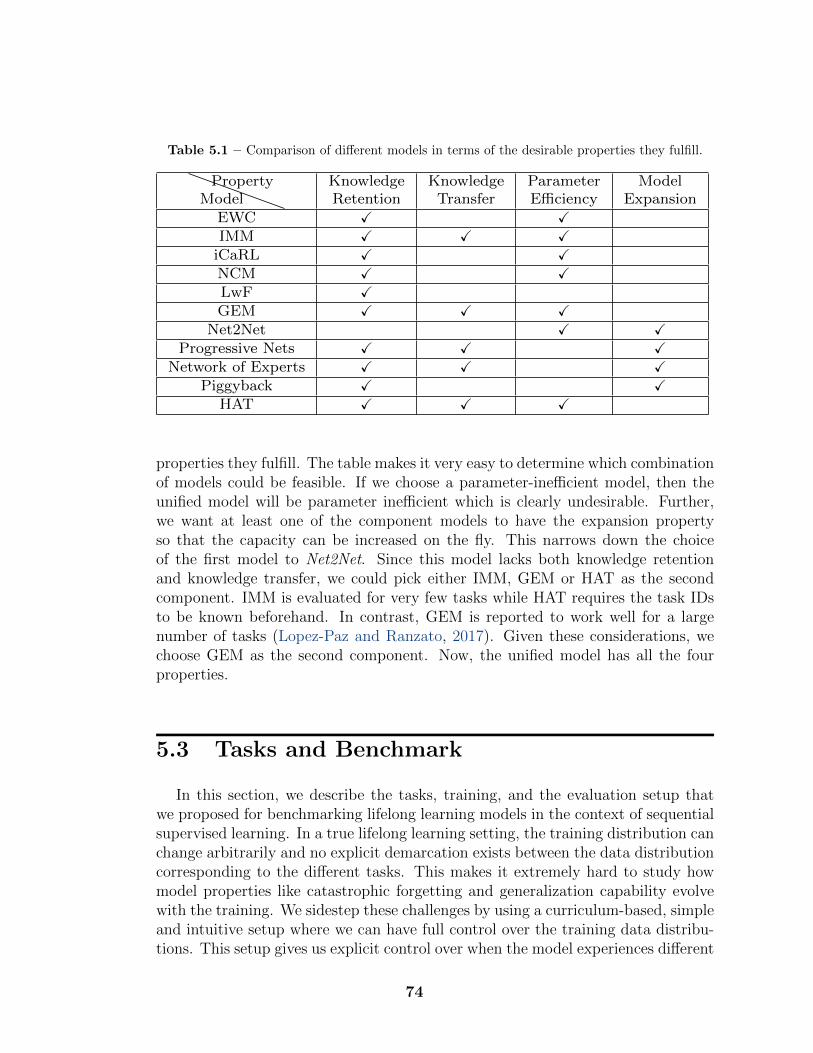
Table 5.1 – Comparison of different models in terms of the desirable properties they fulfill.

ModelProperty Knowledge

RetentionKnowledge

TransferParameterEfficiency

ModelExpansion

EWC X XIMM X X X

iCaRL X XNCM X XLwF XGEM X X X

Net2Net X XProgressive Nets X X X

Network of Experts X X XPiggyback X X

HAT X X X

properties they fulfill. The table makes it very easy to determine which combinationof models could be feasible. If we choose a parameter-inefficient model, then theunified model will be parameter inefficient which is clearly undesirable. Further,we want at least one of the component models to have the expansion propertyso that the capacity can be increased on the fly. This narrows down the choiceof the first model to Net2Net. Since this model lacks both knowledge retentionand knowledge transfer, we could pick either IMM, GEM or HAT as the secondcomponent. IMM is evaluated for very few tasks while HAT requires the task IDsto be known beforehand. In contrast, GEM is reported to work well for a largenumber of tasks (Lopez-Paz and Ranzato, 2017). Given these considerations, wechoose GEM as the second component. Now, the unified model has all the fourproperties.

5.3 Tasks and Benchmark

In this section, we describe the tasks, training, and the evaluation setup thatwe proposed for benchmarking lifelong learning models in the context of sequentialsupervised learning. In a true lifelong learning setting, the training distribution canchange arbitrarily and no explicit demarcation exists between the data distributioncorresponding to the different tasks. This makes it extremely hard to study howmodel properties like catastrophic forgetting and generalization capability evolvewith the training. We sidestep these challenges by using a curriculum-based, simpleand intuitive setup where we can have full control over the training data distribu-tions. This setup gives us explicit control over when the model experiences different

74

data distributions and in what order. Specifically, we train the models in the cur-riculum style setup (Bengio et al., 2009) where the tasks are ordered by difficulty.We discuss the rationale behind using the curriculum approach in section 5.3.5. Weconsider the following three tasks as part of the benchmark.

5.3.1 Copy Task

The copy task is an algorithmic task introduced by Graves et al. (2014) totest whether the training network can learn to store and recall a long sequence ofrandom vectors. Specifically, the network is presented with a sequence of randomlyinitialized, seven-bit vectors. Each such vector is followed by an eighth bit whichserves as a delimiter flag. This flag is zero at all time-steps except for the endof the sequence. The network is trained to generate the entire sequence exceptthe delimiter flag. The different levels are defined by considering input sequencesof different lengths. We start with input sequences of length 5 and increase thesequence length in steps of 3 and go till the maximum sequence length of 62 (20levels). We can consider arbitrarily large sequences but we restrict ourselves tomaximum sequence length of 62 as none of the considered models were able tolearn all these sequences. We report the bit-wise accuracy metric.

5.3.2 Associative Recall Task

The associative recall task is another algorithmic task introduced by Graveset al. (2014). In this task, the network is shown a list of items where each item is asequence of randomly initialized 8-bit binary vectors, bounded on the left and theright by the delimiter symbols. First, the network is shown a sequence of items andthen it is shown one of the items (from the sequence). The model is required tooutput the item that appears next from the ingested sequence. We set the lengthof each item to be 3. The levels are defined in terms of the number of items in thesequence. The first level considers sequences with 5 items and the number of itemsis increased in steps of 3 per level, going till 20 levels where there are 62 items persequence. We report the bit-wise accuracy metric.

5.3.3 Sequential Stroke MNIST Task

The Sequential Stroke MNIST (SSMNIT) task was introduced by Gulcehre et al.(2017) with an emphasis on testing the long-term dependency modeling capabilitiesof RNNs. In this task, each MNIST digit image I is represented as a sequence ofquadruples {dxi, , dyi, eosi, eodi}Ti=1. Here, T is the number of pen strokes needed

75

to define the digit, (dxi, dyi) denotes the pen offset from the previous to the currentstroke (can be 1, -1 or 0), eosi is a binary-valued feature to denote end of strokeand eodi is another binary-valued feature to denote end of the digit. The averagenumber of strokes per digit is 40. Given a sequence of pen-stroke sequences, the taskis to predict the sequence of digits corresponding to each pen-stroke sequences inthe given order. This is an extremely challenging task as the model is first requiredto predict the digits based on the pen-stroke sequence, count the number of digits,and then generate the digits in the same order as the input after having processedthe entire sequence of pen-strokes. The levels are defined in terms of the numberof digits that make up the sequence. Given that this task is more challenging thanthe other two tasks, we use a sequence of length 1 (i.e. single digit sequences) forthe first level and increase the sequence length in steps of 1. Just like before, weconsider 20 levels and report the per-digit accuracy as the metric.

5.3.4 Benchmark

So far, we have considered the setup with three tasks and have defined multiplelevels within each task. Alternatively, we could think of each task as a “task dis-tribution” and each level (within the task) as a task (within a “task distribution”).From now on, we employ the task-distribution / task notation to keep the discussionconsistent with the literature in lifelong learning where multiple tasks are consid-ered. Thus we have 3 task distributions (Copy, Associative Recall, and SSMNIST)and multiple tasks (in increasing order of difficulty) per task distribution. To beclosely aligned with the true lifelong learning setup, we train all the models in anonline manner where the network sees a stream of training data. Further, none ofthe examples are seen more than once. A common setup in online learning is totrain the model with one example at a time. Instead, we train the model usingmini-batches of 10 examples at a time to exploit the computational benefits of us-ing mini-batches. However, we ensure that every mini-batch is generated randomlyand that none of the examples are repeated so that a separate validation or testdataset is not needed. For each task (within a task distribution), we report thecurrent task accuracy as an indicator of the model’s performance on the currenttask. If the running-average of the current task accuracy, averaged over the last kbatches, is greater-than or equal-to c%, the model is said to have learned the taskand we can start training the model on the next task. If the model fails to learn thecurrent task, we stop the training procedure and report the number of tasks com-pleted. Every model is trained for m mini-batches before it is evaluated to checkif it has learned the task. Since we consider models with different capacity, somemodels could learn the task faster thus experiencing fewer examples. This setupensures that each model is trained on the same number of examples. This trainingprocedure is repeated for all the task distributions. Benchmark parameters k, m,

76

and c can be set to any reasonable value, as long as they are kept constant for alltasks in a given task distribution. Specifically, we set k = 100, and m = 10000for all the tasks, as well as c = 80 for Copy and c = 75 for Associative Recall andSSMNIST.

In the lifelong learning setting, it is very important for the model to retain knowl-edge from the previous tasks while generalizing to the new tasks. Hence, each timethe model learns a task, we evaluate it on all the previous tasks (that it has beentrained on so far) and report the model’s performance (in terms of accuracy) foreach of the previous task. Additionally, we also report the average of all these pre-vious task accuracies and denote it as the per-task-previous-accuracy. When themodel fails to learn a task and its training is stopped, we report both the individualper-task-previous-accuracy metrics and the average of these metrics, which is de-noted as the previous-task-accuracy. While the per-task-previous-accuracy metriccan be used as a crude approximation to quantify the effect of catastrophic forget-ting, we highlight that the metric, on its own, is an insufficient metric. Considera model which learns to solve just 1 task and terminates training after the 2nd

task. When evaluated for backward transfer, it would be evaluated only on the 1st

task. Now consider a model which just finished training on the 10th task. Whenevaluated for backward transfer, it would be evaluated on the first 9 tasks. per-task-previous-accuracy metric favors models which stop training early and hencethe series of per-task-previous-accuracy metrics is a more relevant measure.

Another interesting aspect of lifelong learning is the generalization to unseentasks. Analogous to the per-task-previous-accuracy and previous-task-accuracy, weconsider the per-task-future-accuracy and future-task-accuracy. There is no successcriteria associated with this evaluation phase and the metrics are interpreted as aproxy of a model’s ability to generalize to future tasks. In our benchmark, the tasksare closely related, which makes it reasonable to test generalization to new tasks.Note that the benchmark tasks can have levels beyond 20 as well. We limited ourevaluation to 20 levels as none of the models could complete all the levels.

In the context of lifelong learning systems, the model needs to expand its capac-ity once it has saturated, to make sure it can keep learning from the incoming data.We simulate this scenario in our benchmark setting as follows. If the model fails tocomplete a given task, we use some capacity expansion technique and expand theoriginal model into a larger model. Specifically, since we are considering RNNs, weexpand the size of the hidden state matrix. The expanded model is then allowedto train on the current task for 20000 iterations. From there, the expanded modelis evaluated (and trained on subsequent tasks) just like a regular model. If theexpanded model fails on any task, the training is terminated. Note that this ter-mination criterion is a part of our evaluation protocol. In practice, we can expandthe model as many times as we want. In the ablation studies, we consider a casewhere the model is expanded twice.

77

5.3.5 Rationale for using curriculum style setup

For all three task distributions, it can be argued that as the sequence length in-creases, the tasks become more challenging, since the model needs to store/retrievea much longer sequence. Hence, for each task distribution, we define a curriculumof tasks by controlling the length of the input sequences. We note that our exper-imental setup is different from a real-life setting in two ways: First, in real-life, wemay not know beforehand which data point belongs to which data (or task) dis-tribution. Second, in real life, we have no control over the difficulty or complexityof the incoming data points. For the benchmark, we assume perfect knowledge ofwhich data points belong to which task and we assume full control over the datadistribution. This trade-off has several advantages:

1. As the tasks are arranged in increasing order of difficulty, it becomes mucheasier to quantify the change in the model’s performance as the evaluationdata distribution becomes different from the training data distribution.

2. It enables us to extrapolate the capacity of the model with respect to theunseen tasks. If the model is unable to solve the nth task, it is unlikely tosolve any of the subsequent tasks as they are harder than the current task.Thus, we can use the number of tasks solved (while keeping other factorslike optimizer fixed) as an ordinal indicator of the model’s capacity.

3. As the data distribution becomes harder, the model is forced to use moreand more of its capacity to learn the task.

4. In general, given n tasks, there are n! ways of ordering the task and the modelshould be evaluated on all these combinations as the order of training taskscould affect the model’s performance. Having the notion of the curriculumgives us a natural way to order the tasks.

To highlight the fact that curriculum-based training is not trivial, we show theperformance of an LSTM in the SSMNIST task in figure 5.1. We can see thattraining on different tasks makes the model highly susceptible to over-fitting toany given task and less likely to generalize across tasks.

Capacity saturation can happen because of two reasons in our proposed bench-mark:

1. The model is operating in a lifelong learning setting and when the modellearns a new task, it also needs to spend some capacity to retain knowledgeabout the previous tasks.

2. As the sequence length increases, the new tasks require more capacity to belearned.

78

1 2 3 4 5 6 7Task

0.0

0.2

0.4

0.6

0.8

1.0Ac

cura

cy

Previous TasksCurrent TaskFuture Tasks

Figure 5.1 – Per-level accuracy on previous tasks, current task, and future tasks for a 128dimensional LSTM trained in the SSMNIST task distribution by using the curriculum. Themodel heavily overfits to the sequence length.

Given these factors, it is expected that as the model learns new tasks, its capacitywould be strained, thus necessitating solutions that enable the model to increaseits capacity on the fly.

5.4 Model

In this section, we first describe how the rehearsal setup is used in the GEMmodel and how the function preserving transformations can be used in the Net2Netmodel. Next, we describe how we extend the Net2Net model for RNNs. Then, wedescribe how the proposed model leverages both these mechanisms in a unifiedlifelong learning framework.

5.4.1 Gradient Episodic Memory (GEM)

In this section, we provide a brief overview of the Gradient Episodic Memory(Lopez-Paz and Ranzato, 2017) and how it is used for alleviating catastrophicforgetting, while ensuring positive transfer on the previous tasks.

79

The basic idea is to store some input examples corresponding to each task (thatthe model has been trained on so far) in a memory buffer B. In practice, the bufferwould have a fixed size, say Bsize. If we know T , the number of tasks that themodel would encounter, we could reserve Bsize/T number of slots for each task.Alternatively, we could start with the first task, use all the slots for storing theexamples from the first task. Then, as we progress through tasks, we keep reducingthe number of memory slots per task. While selecting the examples to store in thebuffer, we just save the last few examples from each task. Specifically, we storeonly 1 minibatch of examples (10 examples) per task and find that even this smallamount of data is sufficient.

As the model is training on the lth task, care is taken to ensure that the currentgradient updates do not increase the loss on the examples already saved in thememory. This is achieved as follows. Given that the model is training on thelth task, we first compute the parameter gradient with respect to the data forthe current task, which we denote as the current task gradient or as gl. Then aparameter gradient is computed corresponding to each of the previous tasks and isdenoted as the previous task gradient. If the current gradient gl increases the loss onany of the previous tasks, it is projected to the closest gradient gl (where closenessis measured in terms of L2 norm) such that the condition is no more violated.Whether the current task gradient increases the loss on any of the previous taskscan be checked by computing the dot product between current task gradient and theprevious task gradient (corresponding to the given previous task). The projectedgradient update gl can be obtained by solving the following set of equations

minimizegl1

2‖gl − gl‖2

2

subject to 〈gl, gk〉 ≥ 0 for all k < l. (5.1)

To solve (5.1) efficiently, the authors use the primal of a Quadratic Program (QP)with inequality constraints:

minimizez1

2z>Cz + p>z

subject to Az ≥ b, (5.2)

where C ∈ Rp×p, p ∈ Rp, A ∈ R(t−1)×p, and b ∈ Rt−1. The dual problem of (5.2) is:

minimizeu,v1

2u>Cu− b>v

subject to A>v − Cu = p,

v ≥ 0. (5.3)

If (u?, v?) is a solution to (5.3), then there is a solution z? to (5.2) satisfying

80

Cz? = Cu? (Dorn, 1960).

The primal GEM QP (5.1) can be rewritten as:

minimizez1

2z>z − g>z +

1

2g>g

subject to Gz ≥ 0,

where G = −(g1, . . . , gt−1), and the constant term g>g is discarded. This newequation is a QP on p variables (where p is the number of parameters of the neuralnetwork). Since the network could have a lot of parameters, it is not feasible tosolve this equation and the dual of the GEM QP is considered:

minimizev1

2v>GG>v + g>G>v

subject to v ≥ 0, (5.4)

since u = G>v+g and the term g>g is constant. This is a QP on t−1� p variables(where t is the number of observed tasks so far). Solution for the dual problem(5.4), v?, can be used to recover the projected gradient update as g = G>v? + g.The authors recommend adding a small constant γ ≥ 0 to v? as it helps to bias thegradient projection to updates that favoured beneficial backwards transfer.

We refer to this projection step as computing the GEM gradient and the result-ing update as the GEM update. Since the projected gradient is only constrainedto not increase the loss on the previous examples, a beneficial backward transfer ispossible.

There are several downsides of using the GEM model. First, the projection ofcurrent task gradient regularizes the model, thereby decreasing its effective capac-ity. This effect can be seen in figure 5.2 where for all the three task distributions,the green curve (Large LSTM model which does not use the GEM update) con-sistently outperforms the red curve (LSTM model which uses the GEM update)both in terms of current task accuracy and in terms of numbers of tasks completed.We counter this limitation by using functional transformations to enable capacityexpansion. Another downside is the cost - both in terms of computation and mem-ory - of storing and rehearsing over the previous examples. We found that for allour experiments, storing just 10 examples per task is sufficient to get benefit fromthe GEM model. Hence the memory footprint of storing the training examplesis very small and almost negligible as compared to the memory cost of persistingdifferent copies of the model. The computational overhead of computing the GEMgradient could be reduced to some extent by controlling the frequency at which themodel rehearses on the previous examples and future work could look at a moresystematic approach to eliminate or reduce this computational cost.

81

5.4.2 Net2Net

Training a lifelong learning system on a continual stream of data can be seen astraining a model with an infinite amount of data. As the model experiences moreand more data points, the size of its effective training dataset increases and eventu-ally the network would have to expand its capacity to continue training. Net2Net(Chen et al., 2015) proposed a very simple technique, based on function preservingtransformations, to achieve zero-shot knowledge transfer when expanding a small,trained network (referred to as the teacher network) into a large, untrained net-work (referred to as the student network). Given a teacher network represented bythe function y = f(x, θ) (where θ refers to the network parameters), a new set ofparameters φ are chosen such that ∀x, f(x, φ) = g(x, θ). The paper considered twovariants of this approach - Net2WiderNet which increases the width of an existingnetwork and Net2DeeperNet which increases the depth of the existing network.The main benefit of using function-preserving transformations is that the studentnetwork immediately performs as well as the original network without having togo through a period of low performance.

We use the Net2WiderNet for expanding the capacity of the model. The formu-lation of Net2WiderNet is as follows.

Assume that we start with a fully connected network where we want to widenlayers i and i + 1. The weight matrix associated with layer i is W (i) ∈ Rm×n andthat associated with layer i+1 isW (i+1) ∈ Rn×p. Layer i may use any element-wisenon-linearity. When we widen layer i, the weight matrix W (i) expands into U (i) tohave q output units where q > n. Similarly, when we widen layer i+ 1, the weightmatrix W (i+1) expands into U (i+1) to have q input units.

A random mapping function g : {1, 2, · · · , q} → {1, 2, · · · , n}, is defined as:

g(j) =

{j j ≤ nrandom sample from {1, 2, · · ·n} j > n

For expanding W (i), the columns of U (i) are randomly chosen from W (i) usingg as shown:

U(i)k,j = W

(i)k,g(j)

Notice that the first n columns of W (i) are copied directly into U (i).

The rows of U (i+1) are randomly chosen from W (i+1) using g as shown:

U(i+1)j,h =

1

|{x|g(x) = g(j)}|W

(i+1)g(j),h

82

Similar to the previous case, the first n rows of W (i+1) are copied directly intoU (i+1).

The replication factor, (given by 1|{x|g(x)=g(j)}|), is introduced to make sure that

the output of the two models is exactly the same. This procedure can be easilyextended to multiple layers. Similarly, the procedure can be used for expandingconvolutional networks (where layers will have more convolution channels) as con-volution is multiplication by a doubly block circulant matrix).

Once the training network has been expanded, the newly created larger networkcan continue training on the incoming data. In theory, there is no restriction onhow many times the Net2Net transformation is applied, though we limit to usingthe transformation only once for most of our experiments.

While Chen et al. (2015) mention lifelong learning as one of their motivations,they only focused on transfer learning from smaller network to a larger network forthe single-task setup. Secondly, they considered the Net2Net transformation in thecontext of feed-forward and convolutional models. Our work is the first attempt touse Net2Net style function transformations for model expansion in the context oflifelong learning or even for sequential models.

5.4.3 Extending Net2Net for RNNs

In this section, we discuss the applicability of the Net2Net formulation for theRNNs in the context of lifelong learning.

The Net2WiderNet transformation makes two recommendations about the train-ing of the student network. The first is that the learning rate for the student net-work may be reduced by an order of 10. This argument seems useful in the originalsetup in which Net2Net is proposed: training the student model over the same dataon which the teacher model was trained. In the context of lifelong learning, themodel does not see the same data again and the data distribution changes withthe task. Hence the argument about lowering the learning rate does not apply.Our preliminary experiments showed that reducing the learning rate degrades theperformance of the model. Hence we decided not to reduce the learning rate afterthe expansion.

The second and more important recommendation is that a small amount ofrandom noise should be added to the student network to break the symmetry. Inour initial experiments, we found that adding noise is a requirement and the modelwithout noise performs extremely poorly. This is in contrast to the feed-forwardsetting where the model works quite well even without using noise.

In the case of RNNs, when we apply the Net2WiderNet transformation, the

83

condition number of the hidden-to-hidden matrices increases drastically and it be-comes ill-conditioned. Recall that the condition number is defined as the ratio ofthe largest singular value of the matrix to its smallest singular value. The ideal con-dition number would be 1 (as is the case of orthogonal matrices) and ill-conditionednetworks are harder to train. Without adding noise, the condition number becomesinfinity after expansion. This is due to the presence of correlated rows in the ma-trix. One way to get around this problem is to add a small amount of noise whichhelps to precondition the weight matrices and hence reduce their condition number.The issue with adding random noise is that it breaks down the equality conditionand hence comes with a trade-off - A higher amount of random noise reduces thecondition number more (make it better conditioned) but pushes the output of thenewly instantiated student network away from the predictions of the old teachernetwork.

To that end, we propose a simple extension to the noise addition procedurewhich ensures that the output of the student and the teacher networks remainthe same while taking care of the preconditioning aspect. Let us say that we hadthe weight matrix Wm×n which we expanded into Um×p using the Net2WiderNettransformation (where p > n). U would have some columns of W replicated. Letus say that the ith column was replicated j times. Then, we would generate a noisematrix of small random values of size m× j. The columns from this noise matrixwould be added to columns that were replicated from ith column of the input matrixW. The noise matrix is generated such that for any row in the matrix, the sumof elements in that row of the noise matrix is 0. It can be shown mathematicallythat this transformation gives the exact same output as the case of no noise. Wehave to employ this procedure to make sure that the random noise we add sums upto 0. Since the given noise is random, it eliminates the correlation between rowsand columns of the expanded weight matrix. Since the noise sums up to 0, it doesensure that the output of the student network is the same as that of the teachernetwork.

How do we generate a matrix of random values where the sum of values alongeach row is 0? We describe a technique to generate a vector of random numberssuch that the values sum up to 1 and then we can use the technique multiple timesto sample multiple rows to form the matrix. Let us say we want to generate avector of random values of length k such that the values sum to 1. We first samplek − 1 random points in the range (0, 1). Note that all these k − 1 values will besmaller than 1 and larger than 0. We added the numbers 0 and 1 to this sequenceand sort the sequence in the ascending order. This gives us a sorted sequence ofk + 1 points where each point lies in the range [0, 1] with the first value being0 and the last value being 1. We take pairwise difference of values between theadjacent points i.e. (second value - first value), (third value - second value) and soon. Summing up this sequence of values would give us (last value - first value) as

84

all the other terms would cancel out. Since the first value is 0 and the last valueis 1, the sum of the sequence of resulting k points is 1. From this sequence ofnumbers, we can subtract 1/k to each of them and the resulting sequence wouldexactly sum up to 0. These steps are also described in Algorithm 2. Additionally,we scale the noise so that it is in the same range as the magnitude of the weightsof the teacher network. Scaling the noise does not change the sum of the noiseelements as both the positive and the negative elements get scaled by the sameamount and still cancel each other. We use this strategy while using the expansionstep.

Algorithm 2 Generating a random-valued vector of length k where the valuessum to 0

1: procedure Generator(k)2: Sample k − 1 random points in the range (0, 1).3: Add values 0 and 1 to the sequence of sampled values.4: Sort the sequence and create a new sequence by subtracting the pairwise

values from the sorted sequence.5: The resulting sequence of k values will sum to 1 (described in the text).6: From each of the values, subtract 1/k to ensure that the resulting sequence

of random values sums up to 0.

5.4.4 Unified Model

We now describe how we combine the catastrophic forgetting solution (GEM)and the capacity expansion solution (functional transformations) to come up witha more suitable model for lifelong learning. Given a task distribution, we randomlyinitialize a model, reset the episodic memory to be empty and start training themodel on the first task (simplest task). Once a task is learned, the model startstraining on the subsequent, more difficult tasks. When we are training the modelon the lth task, the episodic memory already has some examples corresponding tothe first l − 1 tasks. The current task gradient is projected with respect to theprevious task gradients to ensure that it does not increase the loss associated withany of the examples in the episodic memory. The projected GEM Gradient is usedto update the weights of the model (GEM Update). The model is trained on thecurrent task for a fixed number of iterations. The last m training examples fromthe current task are stored in the episodic memory for use in the subsequent tasks.In general, the m examples can be selected with some more sophisticated strategythough Lopez-Paz and Ranzato (2017) reports, and we validate, that using just thelast m samples works well in practice.

85

If the model completes learning the current task (i.e. achieves a thresholdamount of accuracy after training), the model can start training on the next task.If the model fails to learn the current task, and has not been expanded so far,the model is expanded to a larger model and is allowed to train further on thecurrent task. Once the expanded model is trained, it is re-evaluated to check if ithas learned the task. If it has, the model progresses to the next task, otherwise,the training procedure is terminated. Irrespective of how much is the current taskaccuracy, the model is evaluated on all the tasks - to measure its previous taskaccuracy and future task accuracy.

5.4.5 Analysis of the computational and memory cost ofthe proposed model

As noted in section 5.1, an important desideratum in lifelong learning modelsis that the computational and the memory costs of the model should ideally growsublinearly as the model is trained on new tasks. In the context of our proposedmodel, the computational and memory costs can change in the following ways:

1. The Net2Net component expands the model. In this case, the expandedmodel would take more resources (both in terms of parameters and time)than the earlier model. We note that the expansion step does not happen forevery new task and is performed only when the model’s capacity saturates.This is in contrast to approaches like Rusu et al. (2016) where a new copyof the network is added every time a new task is introduced thus increasingboth the parameters and the compute time linearly with the number of tasks.In our case, the frequency of expansion is sublinear in the number of tasks.

2. The GEM model stores some examples (in a buffer) from the previous tasksand performs gradient computation with respect to those examples, alongwith the gradient computation for the current examples. As noted in sec-tion 5.4.1, we could keep the buffer size to be fixed and replace some examplesfrom the previous tasks as new examples are observed while making sure thatall the tasks are represented through examples in the buffer. In practice, wefound that storing a few examples per task is sufficient to get benefit fromthe GEM model (as also observed by Lopez-Paz and Ranzato (2017)), mak-ing the memory footprint negligible. As noted earlier, future work couldlook at some systematic ways of selecting the examples from the buffer thusreducing the computational overhead.

One beneficial side effect of using Net2Net expansion is the zero-shot knowledgetransfer that further amortizes the cost of training a newly initialized larger model

86

- either from a smaller, pre-trained model or from dataset corresponding to thetasks encountered so far.

5.5 Experiments

5.5.1 Models

For each task distribution, we consider a standard recurrent (LSTM) modeloperating in the lifelong learning setting. We consider the different aspects oftraining a lifelong learning system and describe how the model variants can accountfor these aspects. We start with an LSTM model with hidden state size of 128 andrefer to this model as the small-Lstm model. This model has sufficient capacity tolearn the first few tasks. We start training the (small-Lstm) model as describedin section 5.3.4. To avoid catastrophic forgetting, we could additionally use theGEM update when training the model. The resulting model is referred to as thesmall-Lstm-Gem model. After learning some tasks, the model would have used upall its capacity (since it is retaining the knowledge of the previous tasks as well). Inthis case, we could expand the model’s capacity using the Net2Net transformationand the model with this capability is referred to as the small-Lstm-Gem-Net2Netmodel. This is the model we propose. Alternatively, we could have started thetraining with a larger model (large-Lstm model) and could have used the GEMupdate (large-Lstm-Gem model) to counter forgetting. The strategy of alwaysstarting training with a large network would not work in practice because in thelifelong learning setting we do not know what network would be sufficiently largeto learn all the tasks beforehand. If we start with a very large model, we wouldneed a lot more computational resources to train the model and the model wouldbe very prone to over-fitting. Our proposed model (small-Lstm-Gem-Net2Net) getsaround this problem by increasing the capacity on the fly as and when needed. Forthe large-Lstm model family, we set the size of the hidden layer to be 256. Ourempirical analysis shows that it is possible to expand the models to a size muchlarger than their current size without interfering with the GEM update.

For the performance on the current task, large-Lstm model can be treated asthe gold standard since this model has the largest capacity among all the modelsconsidered. Unlike the models which use the GEM Update, this model does nothave to “use” some of its capacity for retaining the knowledge of the previous tasks.For the performance on the previous tasks (catastrophic forgetting), we consider thelarge-Lstm-Gem model as the gold standard as this model has the largest capacityamong all the models and is specifically designed to counter catastrophic forgetting.

87

While we do not have a gold standard for the Future Task Accuracy, both large-Lstm-Gem and large-Lstm are reasonable models to compare with. Overall, wehave three different gold standards for three setups (and metrics) and we compareour proposed model to these different gold standards (each specialized for a specificuse-case).

5.5.2 Hyper Parameters

All the models are implemented using PyTorch 0.4.1 (Paszke et al., 2017). Adamoptimizer (Kingma and Ba, 2014) is used with a learning rate of 0.001. We usedone layer LSTM models with hidden dimensions of size 128 and 256. Net2Net isused to expand LSTM models of size 128 to 256. For the GEM model, we keep oneminibatch (10 examples) of data per task for obtaining the projected gradients.We follow the guidelines and hyperparameter configurations as specified in therespective papers for both GEM and Net2Net models.

5.5.3 Results

Figure 5.2 shows the trend of the current task accuracy for the different modelson the three task distributions. In these plots, a higher curve corresponds tothe model that has higher accuracy on the current task and models which learnmore tasks are spread out more along the x-axis. We compare the performanceof the proposed model small-Lstm-Gem-Net2Net with the gold standard large-Lstm model. We additionally compare with large-Lstm-Gem model as both thismodel and the proposed model are constrained to use some of their capacity onthe previous tasks. Hence it provides a more realistic estimate of the strengthof the proposed model. It also allows us to study the effect of the GEM Updateon the model’s effective capacity (in terms of the number of tasks cleared). Theblue dotted line corresponds to the expansion step when the model is not able tolearn the current task and had to expand. This shows that using the capacityexpansion technique from Net2Net enables learning on newer tasks. We highlightthat before expansion, the proposed model small-Lstm-Gem-Net2Net had a muchsmaller capacity (128 hidden dims) as compared to the other two models whichstarted with a much larger capacity (256 hidden dims). This explains why thelarger models have much better performance in the initial stages. Post expansion,the proposed model overtakes the GEM based model in all the cases (in terms ofthe number of tasks solved). We can observe that in all the cases, the large-Lstmmodel outperforms the large-Lstm-Gem model, which suggests that using the GemUpdate comes at the cost of reducing the capacity for the current task. Usingcapacity expansion techniques with GEM enables the model to account for this

88

loss of capacity.

0 2 4 6 8 10 12 14Task

0.75

0.80

0.85

0.90

0.95

Accu

racy

0 2 4 6 8 10Task

0.74

0.75

0.76

0.77

Accu

racy

small-Lstm-Gem-Net2Netlarge-Lstmlarge-Lstm-GemExpanding small-Lstm-Gem

2 4 6 8 10 12Task

0.600.650.700.750.800.850.90

Accu

racy

Figure 5.2 – Current Task Accuracy for the different models on the three “task distributions”(Copy, Associative Recall, and SSMNIST respectively). On the x-axis, we plot the index of thetask on which the model is training currently and on the y-axis, we plot the accuracy of themodel on that task. Higher curves have higher current task accuracy and curves extending morehave completed more tasks. For all the three “task distributions”, our proposed small-Lstm-Gem-Net2Net model clears either more levels or same number of levels as the large-Lstm-Gem model.Before the blue dotted line, the proposed model is of much smaller capacity (hidden size of 128)as compare to other two models which have a larger hidden size (256). Hence the larger modelshave better accuracy initially. Capacity expansion technique allows our proposed model to clearmore tasks than it would have cleared otherwise.

Models0.00.10.20.30.40.50.60.70.80.9

Accu

racy

Models0.72

0.73

0.74

0.75

0.76

0.77

Accu

racy

large-Lstmsmall-Lstm-Gem-Net2Netlarge-Lstm-Gem

Models0.00.10.20.30.40.50.60.70.80.9

Accu

racy

Figure 5.3 – Previous Task Accuracy for the different models on the three task distributions(Copy, Associative Recall, and SSMNIST respectively). Different bars represent different modelsand on the y-axis, we plot the average previous task accuracy (averaged for all the tasks thatthe model learned). Higher bars have better accuracy on the previously seen tasks and are morerobust to catastrophic forgetting. For all the three task distributions, the proposed models arevery close in performance to the large-Lstm-Gem models and much better than the large-Lstmmodels.

Figure 5.3 shows the trend of the previous task accuracy for the different mod-els. A higher bar corresponds to better accuracy on the previous tasks (moreresilience to catastrophic forgetting). We compare the performance of the pro-posed model small-Lstm-Gem-Net2Net with the gold standard model large-Lstm-Gem. We additionally compare with the large-Lstm model to demonstrate thatGEM Update is essential to have a good performance on the previous tasks. Themost important observation is the relative performance of the proposed small-Lstm-Gem-Net2Net model and the large-Lstm-Gem model. The small-Lstm-Gem-Net2Net model started as a smaller model, consistently learned more tasks than

89

Models0.4

0.5

0.6

0.7Ac

cura

cylarge-Lstm-Gemsmall-Lstm-Gem-Net2Netlarge-Lstm

Models0.5

0.6

0.7

0.8

Accu

racy

Models0.0

0.1

0.2

0.3

0.4

Accu

racy

Figure 5.4 – Future Task Accuracy for the different models on the three task distributions(Copy, Associative Recall, and SSMNIST respectively). Different bars represent different modelsand on the y-axis, we plot the average future task accuracy (averaged for all the tasks that themodel learned). Higher bars have better accuracy on the previously unseen tasks and are morebeneficial for achieving knowledge transfer to future tasks. Even though the proposed model doesnot have any component for specifically generalizing to the future tasks, we expect the proposedmodel to generalize at least as well as the large-Lstm-Gem model and comparable to large-Lstm.Interestingly, our model outperforms the large-Lstm model for Copy task and is always betterthan (or as good as) the large-Lstm-Gem model.

large-Lstm-Gem model and is still almost as good as large-Lstm-Gem model interms of Previous Task Accuracy. This shows that the proposed model is veryrobust to catastrophic forgetting while being very good at learning the currenttask. We also observe that for all the three “task distributions”, the models usingthe GEM update are more resilient to catastrophic forgetting as compared to themodels without the GEM Update.

Figure 5.4 shows the trend of the future task accuracy for different models. Ahigher bar corresponds to better accuracy on the future (unseen) tasks. Since wedo not have any gold standard for this setup, we consider both large-Lstm-Gemand large-Lstm models as they both are reasonable models to compare with. Thegeneral trend is that our proposed model is quite close to the reference models for2 out of 3 tasks. Note that both the larger models started training with a muchlarger capacity and further, the large-Lstm model is not constrained by the GEMUpdate and hence the maximum amount of effective capacity. This could be onereason why the model can outperform our proposed model for one of the tasks.

We also consider the heatmap plots where we plot the accuracy of differentmodels (for different “task distributions”) as they are trained and evaluated ondifferent tasks. As pointed out in section 5.3.4, the aggregated metrics (current taskaccuracy, previous task accuracy, etc) are not sufficient to compare the performanceof different models and fine-grained analysis is useful for having a holistic view. Weobserve that for the large-Lstm model, the large values are concentrated along thediagonal while for the small-Lstm-Gem-Net2Net and the large-Lstm-Gem models,the high values are concentrated in the lower diagonal region indicating that the twomodels are quite resilient to catastrophic forgetting. Additionally, note that while

90

1 2 3 4 5 6 7 8 9 10 11Training Task

12

34

56

78

910

11Ev

alua

tion

Task

0.5

0.6

0.7

0.8

0.9

1 2 3 4 5 6 7 8 9 10Training Task

12

34

56

78

910

Eval

uatio

n Ta

sk

0.6

0.7

0.8

0.9

1 2 3 4 5 6 7 8 9 10 11 12 13Training Task

12

34

56

78

9101

1121

3Ev

alua

tion

Task

0.5

0.6

0.7

0.8

0.9

(a) Copy Task

1 2 3 4 5 6 7Training Task

12

34

56

7Ev

alua

tion

Task

0.30

0.45

0.60

0.75

0.90

1 2 3 4 5Training Task

12

34

5Ev

alua

tion

Task

0.30

0.45

0.60

0.75

0.90

1 2 3 4 5 6 7 8 9 10 11 12 13Training Task

12

34

56

78

9101

112

Eval

uatio

n Ta

sk

0.15

0.30

0.45

0.60

0.75

0.90

(b) SSMNIST Task

Figure 5.5 – Accuracy of the different models (small-Lstm-Gem-Net2Net, large-Lstm-Gem andlarge-Lstm respectively) as they are trained and evaluated on different tasks for the Copy and theSSMNIST task distributions. On the x-axis, we show the task on which the model is trained andon the y-axis, we show the accuracy corresponding to the different tasks on which the model isevaluated. We observe that for the large-Lstm model, the high accuracy values are concentratedalong the diagonal which indicates that the model does not perform well on the previous task.In the case of both small-Lstm-Gem-Net2Net and large-Lstm-Gem models, the high values arein the lower diagonal region indicating that the two models are quite resilient to catastrophicforgetting.

91

the large-Lstm-Gem model appears to be more resilient to catastrophic forgetting,the small-Lstm-Gem-Net2Net model consistently clears more tasks. Note that eventhough we are evaluating the models for all the tasks in the benchmark, we arerestricting the heatmap to only show evaluation results for the highest task indexthat the model could solve. This results in square-shaped heatmaps which areeasier to analyze.

It is important to note that we are using a single proposed model (small-Lstm-Gem-Net2Net) and comparing it with gold-standard models in 3 different contexts- performance on the current task, performance on the backward tasks and perfor-mance on the future tasks. Our model can provide strong performance on all threetasks by countering catastrophic forgetting and by using capacity expansion.

5.6 Conclusion

In this chapter, we study the problem of capacity saturation and catastrophicforgetting in lifelong learning in the context of sequential supervised learning. Wepropose to unify Gradient Episodic Memory (a catastrophic forgetting alleviationapproach) and Net2Net (a capacity expansion approach) to develop a model thatis more suitable for lifelong learning. We also propose a curriculum based eval-uation benchmark where the models are trained on a task with increasing levelsof difficulty. This enables us to sidestep some of the challenges that arise whenstudying lifelong learning. We conduct experiments on the proposed benchmarktasks and show that the proposed model is better suited for the lifelong learningsetting as compared to the two individual models. As future work, we would wantto address the computational overhead associated with the GEM Update step. Onepotential solution called Averaged GEM has been recently proposed by Chaudhryet al. (2019).

92

6 Discussions and FutureWork

In this final chapter, we summarize the contributions of this thesis and discusssome possible future research directions based on this thesis’s work.

6.1 Summary of Contributions

This thesis focused on the challenges in training Recurrent Neural Networks(RNNs). Specifically, we attempted to tackle the following three fundamental chal-lenges that arise when training RNNs in single-task and multi-task settings:

— Vanishing gradients: When training RNNs with very long sequences, gra-dients vanish for two reasons: recurrent matrix multiplication (due to thelinear chain dependencies on previous hidden states) and saturating activa-tion functions. In Chapter 3, we proposed a recurrent architecture calledTARDIS which is basically an LSTM with dynamic skip connections (akawormhole connections) to the previous hidden states. These dynamic skipconnections create tree-structured dependencies to previous hidden statesrather than linear chain dependencies created in a vanilla LSTM. This helpsin better gradient flow in very long sequences. Chapter 4 proposes anotherrecurrent architecture called Non-saturating Recurrent Unit (NRU). NRUsreplace recurrent multiplicative updates with recurrent additive updates anddoes not have any saturating activation function. Thus NRUs have signifi-cantly better gradient flow when compared to other state-of-the-art recurrentarchitectures.

— Capacity saturation and Catastrophic forgetting: When training RNNsin the lifelong learning setting, where it would see a series of tasks, the per-formance on the previous tasks might degrade while learning the currenttask. This is known as catastrophic forgetting. Catastrophic forgetting couldhappen for two reasons: (i) while trying to find the optimal parameter con-figuration for the current task, the model could move away from the optimalparameter configuration for the previous tasks, (ii) Since we are using afinite capacity parametric model, the network would unlearn some previ-ous task to learn the current task if there is not enough capacity to learn

93

more tasks. This second issue is known as Capacity saturation. While muchof the existing work studies catastrophic forgetting in isolation, Chapter 5stresses that we should study both capacity saturation and catastrophic for-getting together. We specifically propose a new way to train RNNs whichincorporates solutions for solving both capacity saturation (Net2Net) andcatastrophic forgetting (GEM).

6.2 Future Directions

6.2.1 Better Recurrent Architectures

The search for a fully expressive recurrent neural network with no vanishingand exploding problem is not yet over. This thesis proposes few ways to improvethe current recurrent architectures and more research is needed to design an idealrecurrent neural network. The work proposed in this thesis sets up the groundworkby introducing architectural changes to improve RNNs and should be followed upby investigating how to improve the learning algorithm itself.

6.2.2 Exploding gradients

NRUs mitigate the problem of vanishing gradients by using non-saturating ac-tivations but they can still suffer from exploding gradients. Unlike vanishing gra-dients, exploding gradients can be controlled by gradient clipping. Our initialexploration of gradient clipping with NRUs shows that it is not a principled so-lution to have a stable training dynamics and more research is needed to devisebetter ways of handling exploding gradients. While most of the literature is focusedon vanishing gradients, we hypothesise that it is easier to work in the explodinggradients regime than the vanishing gradients regime. We conjecture that oncethe gradient vanishes, there is no hope in learning those long-term dependencies.NRUs and ReLU RNNs could be good starting points for research on explodinggradients.

6.2.3 Do we really need recurrent architectures?

Recently introduced Transformer architecture (Vaswani et al., 2017) is shown tobe superior to the recurrent architectures on several NLP tasks (Liu et al., 2019a,b).Transformer is essentially a feed-forward neural network with self-attention mech-anism. This raises the critical question: do we really need recurrent architectures?

94

In one of our recent work (Sankar et al., 2019), we show that we need both atten-tion and recurrence to model sequential problems. One potential research directionis to combine the benefits on Transformers and RNNs by designing a hybrid se-quence modeling architecture. Some of the recent efforts in this direction includesTransformer-XL (Dai et al., 2019) and Universal Transformers (Dehghani et al.,2019). Another important research initiative would be to design very deep RNNsto compete with the benefits that Transformers gain through their depth. Whiletraining very deep LSTMs would have vanishing gradient issues, deep NRUs shouldreduce the vanishing gradient issue and would be the ideal architecture for this task.

6.2.4 Recurrent Neural Networks for Reinforcement Learn-ing

Learning long-term credit assignment is one of the fundamental problems in Re-inforcement Learning (RL) (Sutton and Barto, 1998). RNNs are primarily used tohandle the partial observability in RL (Heess et al., 2015) though RNNs can be seenas the architectural solution for handling long-term credit assignment. However,dependencies in a typical RL task could be in the order of thousands of time steps.Hence we need recurrent architectures which can model really long-term depen-dencies. NRUs can be considered as the first step towards such powerful recurrentarchitectures. Our initial experiments show that NRUs can model dependenciesof length of order 2000 in the copy task. One immediate step would be to applyNRUs on standard RL tasks with very long dependencies.

6.2.5 Reinforcement Learning for Recurrent Neural Net-works

While the previous subsection suggested using RNNs to model long-term creditassignment problem in RL, we can also transfer the knowledge from the RL litera-ture on the long-term credit assignment problem to learning long-term dependenciesin RNNs. One potential research direction is to look at eligibility traces (Sutton andBarto, 1998) in RL and derive equivalent algorithms for training RNNs. In chapter3, we used REINFORCE to compute approximate gradients for non-differentiablecomponents of TARDIS architecture. A possible extension is to design better waysof computing approximate gradients using RL.

95

6.3 Conclusion

In this thesis, we discussed some of the fundamental challenges in training Re-current Neural Networks. This includes the problems of vanishing gradients, catas-trophic forgetting, and capacity saturation. The thesis has made some progress ineach of these problems by proposing new architectures and training algorithms. Aswe highlighted in the introduction, any improvement to training RNNs should havea significant impact in several real-world sequential problems. We strongly believethat the proposed architectures and algorithms would show such impact.

96

Bibliography

R. Aljundi, P. Chakravarty, and T. Tuytelaars. Expert Gate: Lifelong Learningwith a Network of Experts. ArXiv e-prints, November 2016.

Martın Arjovsky, Amar Shah, and Yoshua Bengio. Unitary evolution recurrentneural networks. In Proceedings of the 33nd International Conference on Ma-chine Learning, ICML 2016, New York City, NY, USA, June 19-24, 2016,pages 1120–1128, 2016.

Jimmy Lei Ba, Jamie Ryan Kiros, and Geoffrey E Hinton. Layer normalization.arXiv preprint arXiv:1607.06450, 2016.

Dzmitry Bahdanau, Jan Chorowski, Dmitriy Serdyuk, Philemon Brakel, andYoshua Bengio. End-to-end attention-based large vocabulary speech recogni-tion. In 2016 IEEE International Conference on Acoustics, Speech and SignalProcessing, ICASSP 2016, Shanghai, China, March 20-25, 2016, pages 4945–4949, 2016. doi: 10.1109/ICASSP.2016.7472618. URL https://doi.org/10.

1109/ICASSP.2016.7472618.

Yoshua Bengio, Patrice Simard, and Paolo Frasconi. Learning long-term depen-dencies with gradient descent is difficult. Neural Networks, IEEE Transactionson, 5(2):157–166, 1994.

Yoshua Bengio, Jerome Louradour, Ronan Collobert, and Jason Weston. Curricu-lum learning. In Proceedings of the 26th annual international conference onmachine learning, pages 41–48. ACM, 2009.

Yoshua Bengio, Nicholas Leonard, and Aaron Courville. Estimating or propagat-ing gradients through stochastic neurons for conditional computation. arXivpreprint arXiv:1308.3432, 2013.

Samuel R Bowman, Gabor Angeli, Christopher Potts, and Christopher D Man-ning. A large annotated corpus for learning natural language inference. arXivpreprint arXiv:1508.05326, 2015.

Andrew Carlson, Justin Betteridge, Bryan Kisiel, Burr Settles, Estevam R Hr-uschka Jr, and Tom M Mitchell. Toward an architecture for never-endinglanguage learning. In AAAI, volume 5, page 3. Atlanta, 2010.

Sarath Chandar, Chinnadhurai Sankar, Eugene Vorontsov, Samira Ebrahimi Ka-hou, and Yoshua Bengio. Towards non-saturating recurrent units for modellinglong-term dependencies. In The Thirty-Third AAAI Conference on Artificial

97

https://doi.org/10.1109/ICASSP.2016.7472618


Intelligence, AAAI 2019, The Thirty-First Innovative Applications of ArtificialIntelligence Conference, IAAI 2019, The Ninth AAAI Symposium on Educa-tional Advances in Artificial Intelligence, EAAI 2019, Honolulu, Hawaii, USA,January 27 - February 1, 2019., pages 3280–3287, 2019. doi: 10.1609/aaai.v33i01.33013280. URL https://doi.org/10.1609/aaai.v33i01.33013280.

A. Chaudhry, P. K. Dokania, T. Ajanthan, and P. H. S. Torr. Riemannian Walkfor Incremental Learning: Understanding Forgetting and Intransigence. arXive-prints, January 2018.

Arslan Chaudhry, Marc’Aurelio Ranzato, Marcus Rohrbach, and Mohamed Elho-seiny. Efficient lifelong learning with A-GEM. In 7th International Conferenceon Learning Representations, ICLR 2019, New Orleans, LA, USA, May 6-9,2019, 2019. URL https://openreview.net/forum?id=Hkf2_sC5FX.

Qian Chen, Xiaodan Zhu, Zhenhua Ling, Si Wei, and Hui Jiang. Enhancing andcombining sequential and tree lstm for natural language inference. arXivpreprint arXiv:1609.06038, 2016.

Tianqi Chen, Ian Goodfellow, and Jonathon Shlens. Net2net: Accelerating learningvia knowledge transfer. arXiv preprint arXiv:1511.05641, 2015.

Jianpeng Cheng, Li Dong, and Mirella Lapata. Long short-term memory-networksfor machine reading. arXiv preprint arXiv:1601.06733, 2016.

Kyunghyun Cho, Bart van Merrienboer, Caglar Gulcehre, Dzmitry Bahdanau,Fethi Bougares, Holger Schwenk, and Yoshua Bengio. Learning phrase repre-sentations using RNN encoder-decoder for statistical machine translation. InProceedings of the 2014 Conference on Empirical Methods in Natural LanguageProcessing, EMNLP 2014, October 25-29, 2014, Doha, Qatar, A meeting ofSIGDAT, a Special Interest Group of the ACL, pages 1724–1734, 2014. URLhttp://aclweb.org/anthology/D/D14/D14-1179.pdf.

Junyoung Chung, Caglar Gulcehre, KyungHyun Cho, and Yoshua Bengio. Em-pirical evaluation of gated recurrent neural networks on sequence modeling.CoRR, abs/1412.3555, 2014. URL http://arxiv.org/abs/1412.3555.

Junyoung Chung, Sungjin Ahn, and Yoshua Bengio. Hierarchical multiscale recur-rent neural networks. arXiv preprint arXiv:1609.01704, 2016.

Tim Cooijmans, Nicolas Ballas, Cesar Laurent, and Aaron C. Courville. Recurrentbatch normalization. CoRR, abs/1603.09025, 2016. URL http://arxiv.org/

abs/1603.09025.

Zihang Dai, Zhilin Yang, Yiming Yang, Jaime G. Carbonell, Quoc Viet Le, andRuslan Salakhutdinov. Transformer-xl: Attentive language models beyond afixed-length context. In Proceedings of the 57th Conference of the Associationfor Computational Linguistics, ACL 2019, Florence, Italy, July 28- August 2,2019, Volume 1: Long Papers, pages 2978–2988, 2019. URL https://www.

aclweb.org/anthology/P19-1285/.

98

https://doi.org/10.1609/aaai.v33i01.33013280

https://openreview.net/forum?id=Hkf2_sC5FX

http://aclweb.org/anthology/D/D14/D14-1179.pdf

http://arxiv.org/abs/1412.3555



https://www.aclweb.org/anthology/P19-1285/


Edwin D. de Jong. Incremental sequence learning. arXiv preprintarXiv:1611.03068, 2016.

Mostafa Dehghani, Stephan Gouws, Oriol Vinyals, Jakob Uszkoreit, and LukaszKaiser. Universal transformers. In 7th International Conference on LearningRepresentations, ICLR 2019, New Orleans, LA, USA, May 6-9, 2019, 2019.URL https://openreview.net/forum?id=HyzdRiR9Y7.

Jia Deng, Wei Dong, Richard Socher, Li-Jia Li, Kai Li, and Li Fei-Fei. Imagenet:A large-scale hierarchical image database. In Computer Vision and PatternRecognition, 2009. CVPR 2009. IEEE Conference on, pages 248–255. Ieee,2009.

William S Dorn. Duality in quadratic programming. Quarterly of Applied Mathe-matics, 18(2):155–162, 1960.

T. Furlanello, Z. C. Lipton, M. Tschannen, L. Itti, and A. Anandkumar. BornAgain Neural Networks. ArXiv e-prints, May 2018.

Felix A. Gers, Jurgen Schmidhuber, and Fred A. Cummins. Learning to forget:Continual prediction with LSTM. Neural Computation, 12(10):2451–2471,2000. doi: 10.1162/089976600300015015. URL https://doi.org/10.1162/

089976600300015015.

Felix A. Gers, Nicol N. Schraudolph, and Jurgen Schmidhuber. Learning precisetiming with LSTM recurrent networks. J. Mach. Learn. Res., 3:115–143, 2002.URL http://jmlr.org/papers/v3/gers02a.html.

Ian Goodfellow, Yoshua Bengio, and Aaron Courville. Deep Learning. MIT Press,2016. http://www.deeplearningbook.org.

Alex Graves, Greg Wayne, and Ivo Danihelka. Neural turing machines. arXivpreprint arXiv:1410.5401, 2014.

Alex Graves, Greg Wayne, Malcolm Reynolds, Tim Harley, Ivo Danihelka, Ag-nieszka Grabska-Barwinska, Sergio G. Colmenarejo, Edward Grefenstette,Tiago Ramalho, John Agapiou, Adria P. Badia, Karl M. Hermann, Yori Zwols,Georg Ostrovski, Adam Cain, Helen King, Christopher Summerfield, PhilBlunsom, Koray Kavukcuoglu, and Demis Hassabis. Hybrid computing us-ing a neural network with dynamic external memory. Nature, advance onlinepublication, October 2016. ISSN 0028-0836. doi: 10.1038/nature20101. URLhttp://dx.doi.org/10.1038/nature20101.

Caglar Gulcehre, Sarath Chandar, Kyunghyun Cho, and Yoshua Bengio. Dynamicneural turing machine with soft and hard addressing schemes. arXiv preprintarXiv:1607.00036, 2016.

Caglar Gulcehre, Sarath Chandar, and Yoshua Bengio. Memory augmented neuralnetworks with wormhole connections. CoRR, abs/1701.08718, 2017. URLhttp://arxiv.org/abs/1701.08718.

99

https://openreview.net/forum?id=HyzdRiR9Y7

https://doi.org/10.1162/089976600300015015

https://doi.org/10.1162/089976600300015015

http://jmlr.org/papers/v3/gers02a.html

http://www.deeplearningbook.org

http://dx.doi.org/10.1038/nature20101


Steven Gutstein, Olac Fuentes, and Eric Freudenthal. Knowledge transfer indeep convolutional neural nets. International Journal on Artificial IntelligenceTools, 17(03):555–567, 2008.

David Ha, Andrew Dai, and Quoc V Le. Hypernetworks. arXiv preprintarXiv:1609.09106, 2016.

Matthew J. Hausknecht and Peter Stone. Deep recurrent q-learning for partiallyobservable mdps. In 2015 AAAI Fall Symposia, Arlington, Virginia, USA,November 12-14, 2015, pages 29–37, 2015. URL http://www.aaai.org/ocs/

index.php/FSS/FSS15/paper/view/11673.

Nicolas Heess, Jonathan J. Hunt, Timothy P. Lillicrap, and David Silver. Memory-based control with recurrent neural networks. CoRR, abs/1512.04455, 2015.URL http://arxiv.org/abs/1512.04455.

Mikael Henaff, Arthur Szlam, and Yann LeCun. Recurrent orthogonal networksand long-memory tasks. In Proceedings of the 33nd International Conferenceon Machine Learning, ICML 2016, 2016.

Geoffrey Hinton, Oriol Vinyals, and Jeff Dean. Distilling the knowledge in a neuralnetwork. arXiv preprint arXiv:1503.02531, 2015.

Sepp Hochreiter. Untersuchungen zu dynamischen neuronalen netzen. Diploma,Technische Universitat Munchen, page 91, 1991.

Sepp Hochreiter and Jurgen Schmidhuber. Long short-term memory. Neural Com-putation, 9(8):1735–1780, 1997.

Sergey Ioffe and Christian Szegedy. Batch normalization: Accelerating deep net-work training by reducing internal covariate shift. CoRR, abs/1502.03167,2015. URL http://arxiv.org/abs/1502.03167.

Eric Jang, Shixiang Gu, and Ben Poole. Categorical reparameterization withgumbel-softmax. arXiv preprint arXiv:1611.01144, 2016.

Li Jing, Caglar Gulcehre, John Peurifoy, Yichen Shen, Max Tegmark, Marin Sol-jacic, and Yoshua Bengio. Gated orthogonal recurrent units: On learning toforget. CoRR, abs/1706.02761, 2017a.

Li Jing, Yichen Shen, Tena Dubcek, John Peurifoy, Scott A. Skirlo, Yann LeCun,Max Tegmark, and Marin Soljacic. Tunable efficient unitary neural networks(EUNN) and their application to rnns. In Proceedings of the 34th InternationalConference on Machine Learning, ICML 2017, Sydney, NSW, Australia, 6-11August 2017, pages 1733–1741, 2017b.

Rafal Jozefowicz, Wojciech Zaremba, and Ilya Sutskever. An empirical explo-ration of recurrent network architectures. In Proceedings of the 32nd Inter-national Conference on Machine Learning, ICML 2015, Lille, France, 6-11July 2015, pages 2342–2350, 2015. URL http://proceedings.mlr.press/

v37/jozefowicz15.html.

100

http://www.aaai.org/ocs/index.php/FSS/FSS15/paper/view/11673

http://www.aaai.org/ocs/index.php/FSS/FSS15/paper/view/11673



http://proceedings.mlr.press/v37/jozefowicz15.html

http://proceedings.mlr.press/v37/jozefowicz15.html

D. P. Kingma and J. Ba. Adam: A Method for Stochastic Optimization. ArXive-prints, December 2014.

J. Kirkpatrick, R. Pascanu, N. Rabinowitz, J. Veness, G. Desjardins, A. A.Rusu, K. Milan, J. Quan, T. Ramalho, A. Grabska-Barwinska, D. Hassabis,C. Clopath, D. Kumaran, and R. Hadsell. Overcoming catastrophic forgettingin neural networks. ArXiv e-prints, December 2016.

Jan Koutnik, Klaus Greff, Faustino Gomez, and Juergen Schmidhuber. A clockworkrnn. arXiv preprint arXiv:1402.3511, 2014.

Alex Krizhevsky, Ilya Sutskever, and Geoffrey E. Hinton. Imagenet classificationwith deep convolutional neural networks. In Advances in Neural InformationProcessing Systems 25: 26th Annual Conference on Neural Information Pro-cessing Systems 2012. Proceedings of a meeting held December 3-6, 2012, LakeTahoe, Nevada, United States., pages 1106–1114, 2012.

David Krueger, Tegan Maharaj, Janos Kramar, Mohammad Pezeshki, NicolasBallas, Nan Rosemary Ke, Anirudh Goyal, Yoshua Bengio, Hugo Larochelle,Aaron Courville, et al. Zoneout: Regularizing rnns by randomly preservinghidden activations. arXiv preprint arXiv:1606.01305, 2016.

Cesar Laurent, Gabriel Pereyra, Philemon Brakel, Ying Zhang, and Yoshua Ben-gio. Batch normalized recurrent neural networks. In 2016 IEEE InternationalConference on Acoustics, Speech and Signal Processing, ICASSP 2016, Shang-hai, China, March 20-25, 2016, pages 2657–2661, 2016. doi: 10.1109/ICASSP.2016.7472159. URL https://doi.org/10.1109/ICASSP.2016.7472159.

Quoc V. Le, Navdeep Jaitly, and Geoffrey E. Hinton. A simple way to initializerecurrent networks of rectified linear units. CoRR, abs/1504.00941, 2015.

Yann LeCun, Yoshua Bengio, and Geoffrey E. Hinton. Deep learning. Nature, 521(7553):436–444, 2015. doi: 10.1038/nature14539. URL https://doi.org/10.

1038/nature14539.

Sang-Woo Lee, Jin-Hwa Kim, Jaehyun Jun, Jung-Woo Ha, and Byoung-Tak Zhang. Overcoming catastrophic forgetting by incremental mo-ment matching. In I. Guyon, U. V. Luxburg, S. Bengio, H. Wal-lach, R. Fergus, S. Vishwanathan, and R. Garnett, editors, Advancesin Neural Information Processing Systems 30, pages 4652–4662. Cur-ran Associates, Inc., 2017. URL http://papers.nips.cc/paper/

7051-overcoming-catastrophic-forgetting-by-incremental-moment-matching.

pdf.

Zhizhong Li and Derek Hoiem. Learning without forgetting. In European Confer-ence on Computer Vision, pages 614–629. Springer, 2016.

Xialei Liu, Marc Masana, Luis Herranz, Joost Van de Weijer, Antonio M Lopez,and Andrew D Bagdanov. Rotate your networks: Better weight consolidationand less catastrophic forgetting. arXiv preprint arXiv:1802.02950, 2018.

101


https://doi.org/10.1038/nature14539

https://doi.org/10.1038/nature14539

http://papers.nips.cc/paper/7051-overcoming-catastrophic-forgetting-by-incremental-moment-matching.pdf



Xiaodong Liu, Pengcheng He, Weizhu Chen, and Jianfeng Gao. Multi-task deepneural networks for natural language understanding. In Proceedings of the57th Conference of the Association for Computational Linguistics, ACL 2019,Florence, Italy, July 28- August 2, 2019, Volume 1: Long Papers, pages 4487–4496, 2019a. URL https://www.aclweb.org/anthology/P19-1441/.

Xiaodong Liu, Pengcheng He, Weizhu Chen, and Jianfeng Gao. Improving multi-task deep neural networks via knowledge distillation for natural language un-derstanding. CoRR, abs/1904.09482, 2019b. URL http://arxiv.org/abs/

1904.09482.

Vincenzo Lomonaco and Davide Maltoni. Core50: a new dataset and benchmarkfor continuous object recognition. In Sergey Levine, Vincent Vanhoucke, andKen Goldberg, editors, Proceedings of the 1st Annual Conference on RobotLearning, volume 78 of Proceedings of Machine Learning Research, pages 17–26. PMLR, 13–15 Nov 2017. URL http://proceedings.mlr.press/v78/

lomonaco17a.html.

David Lopez-Paz and Marc Aurelio Ranzato. Gradient episodic mem-ory for continual learning. In I. Guyon, U. V. Luxburg, S. Bengio,H. Wallach, R. Fergus, S. Vishwanathan, and R. Garnett, editors, Ad-vances in Neural Information Processing Systems 30, pages 6467–6476.Curran Associates, Inc., 2017. URL http://papers.nips.cc/paper/

7225-gradient-episodic-memory-for-continual-learning.pdf.

Sergey Loyka. On singular value inequalities for the sum of two matrices. arXivpreprint arXiv:1507.06630, 2015.

Chris J Maddison, Andriy Mnih, and Yee Whye Teh. The concrete distribu-tion: A continuous relaxation of discrete random variables. arXiv preprintarXiv:1611.00712, 2016.

Arun Mallya, Dillon Davis, and Svetlana Lazebnik. Piggyback: Adapting a singlenetwork to multiple tasks by learning to mask weights. In Proceedings of theEuropean Conference on Computer Vision (ECCV), pages 67–82, 2018.

Mitchell P. Marcus, Beatrice Santorini, and Mary Ann Marcinkiewicz. Building alarge annotated corpus of english: The penn treebank. Computational Lin-guistics, 19(2):313–330, 1993.

Michael McCloskey and Neal J Cohen. Catastrophic interference in connectionistnetworks: The sequential learning problem. In Psychology of learning andmotivation, volume 24, pages 109–165. Elsevier, 1989.

Thomas Mensink, Jakob Verbeek, Florent Perronnin, and Gabriela Csurka. Metriclearning for large scale image classification: Generalizing to new classes atnear-zero cost. In Computer Vision–ECCV 2012, pages 488–501. Springer,2012.

102




http://proceedings.mlr.press/v78/lomonaco17a.html

http://proceedings.mlr.press/v78/lomonaco17a.html

http://papers.nips.cc/paper/7225-gradient-episodic-memory-for-continual-learning.pdf

http://papers.nips.cc/paper/7225-gradient-episodic-memory-for-continual-learning.pdf

Stephen Merity, Nitish Shirish Keskar, and Richard Socher. Regularizing andoptimizing LSTM language models. CoRR, abs/1708.02182, 2017. URLhttp://arxiv.org/abs/1708.02182.

Tomas Mikolov, Ilya Sutskever, Anoop Deoras, Hai-Son Le, Stefan Kombrink,and J Cernocky. Subword language modeling with neural networks. preprint(http://www. fit. vutbr. cz/imikolov/rnnlm/char. pdf), 2012.

Andriy Mnih and Karol Gregor. Neural variational inference and learning in beliefnetworks. arXiv preprint arXiv:1402.0030, 2014.

Volodymyr Mnih, Nicolas Heess, Alex Graves, and Koray Kavukcuoglu. Re-current models of visual attention. In Advances in Neural Informa-tion Processing Systems 27: Annual Conference on Neural Informa-tion Processing Systems 2014, December 8-13 2014, Montreal, Quebec,Canada, pages 2204–2212, 2014. URL http://papers.nips.cc/paper/

5542-recurrent-models-of-visual-attention.

Volodymyr Mnih, Adria Puigdomenech Badia, Mehdi Mirza, Alex Graves, Tim-othy P. Lillicrap, Tim Harley, David Silver, and Koray Kavukcuoglu. Asyn-chronous methods for deep reinforcement learning. In Proceedings of the 33ndInternational Conference on Machine Learning, ICML 2016, New York City,NY, USA, June 19-24, 2016, pages 1928–1937, 2016.

Vinod Nair and Geoffrey E Hinton. Rectified linear units improve restricted boltz-mann machines. In Proceedings of the 27th international conference on ma-chine learning (ICML-10), pages 807–814, 2010.

Junier B. Oliva, Barnabas Poczos, and Jeff G. Schneider. The statistical recurrentunit. In Proceedings of the 34th International Conference on Machine Learn-ing, ICML 2017, Sydney, NSW, Australia, 6-11 August 2017, pages 2671–2680,2017.

Razvan Pascanu, Caglar Gulcehre, Kyunghyun Cho, and Yoshua Bengio. How toconstruct deep recurrent neural networks. arXiv preprint arXiv:1312.6026,2013a.

Razvan Pascanu, Tomas Mikolov, and Yoshua Bengio. On the difficulty of trainingrecurrent neural networks. ICML (3), 28:1310–1318, 2013b.

Adam Paszke, Sam Gross, Soumith Chintala, Gregory Chanan, Edward Yang,Zachary DeVito, Zeming Lin, Alban Desmaison, Luca Antiga, and AdamLerer. Automatic differentiation in pytorch. In NIPS-W, 2017.

Jack W. Rae, Jonathan J. Hunt, Tim Harley, Ivo Danihelka, Andrew W.Senior, Greg Wayne, Alex Graves, and Timothy P. Lillicrap. Scalingmemory-augmented neural networks with sparse reads and writes. CoRR,abs/1610.09027, 2016.

103


http://papers.nips.cc/paper/5542-recurrent-models-of-visual-attention

http://papers.nips.cc/paper/5542-recurrent-models-of-visual-attention

Sylvestre-Alvise Rebuffi, Alexander Kolesnikov, Georg Sperl, and Christoph HLampert. icarl: Incremental classifier and representation learning. In Proc.CVPR, 2017.

Mark B Ring. Child: A first step towards continual learning. Machine Learning,28(1):77–104, 1997.

Tim Rocktaschel, Edward Grefenstette, Karl Moritz Hermann, Tomas Kocisky,and Phil Blunsom. Reasoning about entailment with neural attention. arXivpreprint arXiv:1509.06664, 2015.

Adriana Romero, Nicolas Ballas, Samira Ebrahimi Kahou, Antoine Chassang,Carlo Gatta, and Yoshua Bengio. Fitnets: Hints for thin deep nets. arXivpreprint arXiv:1412.6550, 2014.

Andrei A Rusu, Neil C Rabinowitz, Guillaume Desjardins, Hubert Soyer, JamesKirkpatrick, Koray Kavukcuoglu, Razvan Pascanu, and Raia Hadsell. Pro-gressive neural networks. arXiv preprint arXiv:1606.04671, 2016.

Chinnadhurai Sankar, Sandeep Subramanian, Chris Pal, Sarath Chandar, andYoshua Bengio. Do neural dialog systems use the conversation history ef-fectively? an empirical study. In Proceedings of the 57th Conference ofthe Association for Computational Linguistics, ACL 2019, Florence, Italy,July 28- August 2, 2019, Volume 1: Long Papers, pages 32–37, 2019. URLhttps://www.aclweb.org/anthology/P19-1004/.

Adam Santoro, Sergey Bartunov, Matthew Botvinick, Daan Wierstra, and TimothyLillicrap. One-shot learning with memory-augmented neural networks. arXivpreprint arXiv:1605.06065, 2016.

Stanislau Semeniuta, Aliaksei Severyn, and Erhardt Barth. Recurrent dropoutwithout memory loss. arXiv preprint arXiv:1603.05118, 2016.

Iulian Vlad Serban, Alessandro Sordoni, Ryan Lowe, Laurent Charlin, JoellePineau, Aaron C. Courville, and Yoshua Bengio. A hierarchical latentvariable encoder-decoder model for generating dialogues. In Proceedingsof the Thirty-First AAAI Conference on Artificial Intelligence, February 4-9, 2017, San Francisco, California, USA., pages 3295–3301, 2017. URLhttp://aaai.org/ocs/index.php/AAAI/AAAI17/paper/view/14567.

J. Serra, D. Surıs, M. Miron, and A. Karatzoglou. Overcoming catastrophic for-getting with hard attention to the task. arXiv e-prints, January 2018.

Daniel L Silver and Robert E Mercer. The task rehearsal method of life-long learn-ing: Overcoming impoverished data. In Conference of the Canadian Societyfor Computational Studies of Intelligence, pages 90–101. Springer, 2002.

Daniel L Silver, Qiang Yang, and Lianghao Li. Lifelong machine learning systems:Beyond learning algorithms. In AAAI Spring Symposium: Lifelong MachineLearning, volume 13, page 05, 2013.

104


http://aaai.org/ocs/index.php/AAAI/AAAI17/paper/view/14567

Shagun Sodhani, Sarath Chandar, and Yoshua Bengio. On training recurrent neuralnetworks for lifelong learning. Neural Computation, 2019.

Ray J Solomonoff. A system for incremental learning based on algorithmic proba-bility. In Proceedings of the Sixth Israeli Conference on Artificial Intelligence,Computer Vision and Pattern Recognition, pages 515–527, 1989.

Sainbayar Sukhbaatar, Arthur Szlam, Jason Weston, and Rob Fergus. End-to-endmemory networks. arXiv preprint arXiv:1503.08895, 2015.

Ilya Sutskever, James Martens, and Geoffrey E Hinton. Generating text withrecurrent neural networks. In Proceedings of the 28th International Conferenceon Machine Learning (ICML-11), pages 1017–1024, 2011.

Ilya Sutskever, Oriol Vinyals, and Quoc V. Le. Sequence to sequence learning withneural networks. In Advances in Neural Information Processing Systems 27:Annual Conference on Neural Information Processing Systems 2014, December8-13 2014, Montreal, Quebec, Canada, pages 3104–3112, 2014.

Richard S. Sutton and Andrew G. Barto. Introduction to Reinforcement Learning.MIT Press, Cambridge, MA, USA, 1st edition, 1998. ISBN 0262193981.

Corentin Tallec and Yann Ollivier. Can recurrent neural networks warp time? In6th International Conference on Learning Representations, ICLR 2018, Van-couver, BC, Canada, April 30 - May 3, 2018, Conference Track Proceedings,2018. URL https://openreview.net/forum?id=SJcKhk-Ab.

Sebastian Thrun. Explanation-based neural network learning. In Explanation-Based Neural Network Learning, pages 19–48. Springer, 1996.

Sebastian Thrun. Lifelong learning algorithms. In Learning to learn, pages 181–209.Springer, 1998.

Sebastian Thrun. Explanation-based neural network learning: A lifelong learningapproach, volume 357. Springer Science & Business Media, 2012.

Endel Tulving. Chronesthesia: Conscious awareness of subjective time. 2002.

Jos van der Westhuizen and Joan Lasenby. The unreasonable effectiveness of theforget gate. CoRR, abs/1804.04849, 2018. URL http://arxiv.org/abs/

1804.04849.

Ashish Vaswani, Noam Shazeer, Niki Parmar, Jakob Uszkoreit, Llion Jones,Aidan N. Gomez, Lukasz Kaiser, and Illia Polosukhin. Attention is allyou need. In Advances in Neural Information Processing Systems 30: An-nual Conference on Neural Information Processing Systems 2017, 4-9 De-cember 2017, Long Beach, CA, USA, pages 5998–6008, 2017. URL http:

//papers.nips.cc/paper/7181-attention-is-all-you-need.

Oriol Vinyals and Quoc V. Le. A neural conversational model. CoRR,abs/1506.05869, 2015. URL http://arxiv.org/abs/1506.05869.

105

https://openreview.net/forum?id=SJcKhk-Ab



http://papers.nips.cc/paper/7181-attention-is-all-you-need

http://papers.nips.cc/paper/7181-attention-is-all-you-need


Eugene Vorontsov, Chiheb Trabelsi, Samuel Kadoury, and Chris Pal. On orthogo-nality and learning recurrent networks with long term dependencies. In Pro-ceedings of the 34th International Conference on Machine Learning, ICML2017, 2017.

Jason Weston, Sumit Chopra, and Antoine Bordes. Memory networks. In Pro-ceedings Of The International Conference on Representation Learning (ICLR2015), 2015. In Press.

Ronald J. Williams. Simple statistical gradient-following algorithms for connec-tionist reinforcement learning. Machine Learning, 8:229–256, 1992.

Scott Wisdom, Thomas Powers, John R. Hershey, Jonathan Le Roux, and Les E.Atlas. Full-capacity unitary recurrent neural networks. In Advances in NeuralInformation Processing Systems 29: Annual Conference on Neural Informa-tion Processing Systems 2016, December 5-10, 2016, Barcelona, Spain, pages4880–4888, 2016.

Yonghui Wu, Mike Schuster, Zhifeng Chen, Quoc V. Le, Mohammad Norouzi,Wolfgang Macherey, Maxim Krikun, Yuan Cao, Qin Gao, Klaus Macherey,Jeff Klingner, Apurva Shah, Melvin Johnson, Xiaobing Liu, Lukasz Kaiser,Stephan Gouws, Yoshikiyo Kato, Taku Kudo, Hideto Kazawa, Keith Stevens,George Kurian, Nishant Patil, Wei Wang, Cliff Young, Jason Smith, JasonRiesa, Alex Rudnick, Oriol Vinyals, Greg Corrado, Macduff Hughes, and Jef-frey Dean. Google’s neural machine translation system: Bridging the gapbetween human and machine translation. CoRR, abs/1609.08144, 2016. URLhttp://arxiv.org/abs/1609.08144.

Bing Xu, Naiyan Wang, Tianqi Chen, and Mu Li. Empirical evaluation of rectifiedactivations in convolutional network. arXiv preprint arXiv:1505.00853, 2015.

Wojciech Zaremba and Ilya Sutskever. Reinforcement learning neural turing ma-chines. CoRR, abs/1505.00521, 2015.

F. Zenke, B. Poole, and S. Ganguli. Continual Learning Through Synaptic Intelli-gence. arXiv e-prints, March 2017.

Julian Georg Zilly, Rupesh Kumar Srivastava, Jan Koutnık, and Jurgen Schmid-huber. Recurrent highway networks. arXiv preprint arXiv:1607.03474, 2016.

106


on challenges in training recurrent neural networkssarathchandar.in/paper/chandar_phd_thesis.pdf ·...

Documents