on choice in a complex environment choice in a complex environment murali agastya...
TRANSCRIPT

On choice in a complex environment
Murali Agastya ∗
Arkadii Slinko †
April 20, 2009
Abstract
A Decision Maker (DM) must choose at discrete moments from a finite set of actionsthat result in random rewards. The environment is complex in that she finds it impos-sible to describe the states and is thus prevented from application of standard Bayesianmethods. This paper presents an axiomatic theory of choice in such environments.
Our approach is to postulate that the DM has a preference relation defined directlyover the set of actions which is updated over time in response to the observed rewards.Three simple axioms that highlight the independence of the given actions, the boundedrationality of the agent, and the principle of insufficient reason at margin are necessaryand sufficient for the DM’s preferences to admit a utility representation. The DM’sbehavior in this case will be akin to fictitious play. We then show that, if rewards aredrawn by a stationary stochastic process, the observed behavior of such a DM almostsurely cannot be distinguished from anyone who is fully cognizant of the environment.
Keywords: Ex-post utility maximization, Choice under ignorance, Multisets, Fictitiousplay.
∗Murali Agastya, Economics Discipline, H04 Merewether Building University of Sydney NSW 2006AUSTRALIA†A.M.Slinko, Department of Mathematics, University of Auckland, Private Bag 92019, Auckland NEW
ZEALAND
1

1 Introduction
Consider a Decision Maker (DM) who has to repeatedly choose from a finite set of actions.Each action results in a random reward, also drawn from a finite set. The environment iscomplex in the sense that the DM is either unable to offer a complete description of thestates of the world or is unable to construct a meaningful prior probability distribution.Naturally, the well established Bayesian methods of, say Savage (1954) or Anscombe andAumann (1963), would then be inapplicable.1 Yet, decision makers often find themselvesin these situations and do somehow make choices, the complexity of the environmentnotwithstanding. This paper offers a theory of choice in such environments.
Our approach is to postulate that the DM has a preference relation defined directlyover the set of actions which is updated over time in response to the sequences of observedrewards. Thus, if A denotes the set of all actions and H the set of all histories, the DM iscompletely described by the family D := (�ht)ht∈H , where �ht is a well defined preferencerelation on the actions following a history ht at date t. A history consists of the sequencesof rewards, drawn from a finite set R, that are obtained over time to each of the actions.We impose axioms on D.
There is a considerable literature in economics and psychology on a variety of “stimulus-response” models of individual choice behavior. In these models, the DM does not attemptto learn the environment, instead she looks at the past experiences and takes her decisionsusing a rule of thumb. To use a term coined by Reinhard Selten, the DM indulges inex-post rational behavior.2 In this literature, the “stimulus” is almost always modeled as areal number which is interpreted as a monetary payoff or an exogenously specified cardinalutility assignment to a reward. The rule that maps these past payoffs to actions is eitherfully specified or is assumed to have some desirable properties. The focus is the analysisof implied adaptive dynamics. These imputed rules of updating vary widely. They rangefrom modifications of fictitious play and reinforcement learning to imitation of peers etc.See for example Borgers, Morales, and Sarin (2004), Schlag (1998), Gigerenzer and Selten
1Knight (1921) and Ellsberg (1961) concern the existence of a prior. More recent and a more directquestioning of the assumption that a DM may have a well defined state space (let alone a known prior)have lead to Gilboa and Schmeidler (1995), Easley and Rustichini (1999), Dekel, Lipman, and Rustichini(2001), Gilboa and Schmeidler (2003) and Karni (2006) among others. Gilboa and Schmeidler (1995), inparticular, forcefully argues how in many environments there is no naturally given state space and how thelanguage of expected utility theory precludes its application in these cases.
2See Selten (2001) and the informal discussion available at http://www.strategy-business.com/press/16635507/05209.
1
(2001), Fudenberg and Levine (1998) and the references therein.An exception to the above is Easley and Rustichini (1999) (hereafter ER). Instead
of directly assuming rules that map payoffs to actions, ER, like us, consider an abstractindividual decision problem modeled as a family of preference relations, not on actions buton lotteries over them, and impose axioms on it. The use of the axiomatic approach todynamic choice under ignorance makes ER the closest relative of this paper. We defer acomplete discussion of the relation of this work to ER (and other literature) to Section 7.We do note here however that there are significant differences both in the formal modelingdetails and in the conceptual basis for the axioms. For instance, our formulation allowsfor considerable path dependence of the DM’s preferences over actions across time whichis ruled out in ER. Our results will also show that the DM can be initially ambiguous onhow to value the rewards but becomes increasingly precise over time. This feature too isabsent in ER (since they also assume that rewards/payoffs are monetary). In fact, theclass of adaptive learning procedures that are axiomatized here resemble fictitious play incontrast to the replicator dynamics characterized in their work.3
What we do share with ER and many of the works cited above is that the DM operatesin a social environment in which there are other decision makers. For, we assume that ateach date the DM is able to observe rewards that occur to each of the actions, includingthose that she herself did not choose. Such an assumption on observability of rewards seemsparticularly natural for situations such as betting on horses or investing on a share-market.For, in these cases there is a sufficient diversity of preferences so that all the actions arechosen in each period by various individuals and outcomes are publicly observable.
There are three results in the main — Theorem 1 is a “utility representation” resultfor D. Theorem 2 uses the previous result to show that the observed behavior of a DMwho obeys our axioms is virtually indistinguishable from a fully rational DM providedthe rewards are generated by a stationary stochastic process. Proposition 3 is a simpleempirical test for refuting the axioms. The novelty in the proof of Theorem 1 is theidentification of a certain isomorphism between preferences over actions across time and abinary relation over multisets of rewards. We then prove Proposition 2, a representationresult for orderings of multisets — a technical result which we expect to be of independentinterest with applications elsewhere in Decision Theory and Social Choice. Theorem 1 isthen deduced from Proposition 2. We shall now elaborate on the axioms and these results.
3Fictitious play was introduced by Brown (1951). See Fudenberg and Levine (1998) for variations offictitious play. See Hopkins (2002) for a nice comparison of fictitious play and replicator dynamics.
2

There are three axioms. The first axiom requires that a comparison of a pair of actionsat any date depends on the historical sequence of observed rewards corresponding to onlythat pair. The second axiom captures the bounded rationality of the DM. It insists thatfor any sequence of rewards attributed to an action in any history, the DM is able to trackonly the number of times various rewards have accrued. The final axiom concerns theupdating of preferences in response to the rewards and is loosely based on the principleof insufficient reason: if a pair of actions receive the same reward in the current periodfollowing a history ht, then their current relative ranking is carried forward to the nextperiod.
One way of ranking actions that would satisfy the above axioms would be for the DMto assign utility weights to the underlying set of rewards and, just as in fictitious play, theutility of an action at any date is the average utility of the rewards that have occured tothe action until then. Our first result, Theorem 1 in Section 2, shows the above axioms areequivalent to precisely this procedure with the following caveat. The set of endogenouslydetermined utility weights for rewards that are available to the DM at any date are notnecessarily unique (even after applying positive affine transformations). Rather, the DMcan choose the utility weights for the rewards from a certain convex polytope Ut in Rn
for each date t such that Ut+1 ⊆ Ut. It is worth noting that the non-uniqueness in thevaluation of rewards coexists with the DM’s preferences over actions being complete andtransitive at every date.
We refer to the above axiomatized procedure as ex-post rationality. Thus, in a nut-shell, Theorem 1 shows that our axioms are equivalent to the agent choosing between theempirical distributions of the rewards to different actions as if she is an expected utilitymaximiser. The fact that Ut+1 ⊆ Ut means an ex-post rational DM learns more about herimputed utilities for the rewards over time.
The simultaneous determination of both the value of rewards and the ranking of actionsover time given by Theorem 1 sets our work apart from the existing literature on dynamiclearning procedures cited previously. Moreover the evolution of utility weights permittedby our result shows that our framework allows for classes of behavior that are not usuallycaptured in the above literature. For instance,4 in evaluating a pair of treatments (ac-tions), suppose a doctor finds the first action has resulted in much better outcomes in the
4This example is related to one given in Gilboa and Schmeidler (2003) who attribute it to Peyton Youngwhen discussing scenarios where their Combination Axiom fails. Their Combination Axiom is related toAxiom 3 here.
3

past but most recently has resulted in a fatality. The second action has no such record.Then, in our framework, even with a single such outcome, it is consistent for the doctorto strictly prefer the second action. That is, in our framework, it is possible that somerewards are implicitly considered to be “infinitely” more relevant than others.
The intersection of all polytopes of the sequence (Ut)t≥1 is always a singleton. How-ever, it does not necessarily constitute a valid assignment of utility weights to the rewards.In the event it does, just this one vector of utility weights may be used to describe theDM’s behavior in all time periods. In this case, the DM is said to admit a “global utilityrepresentation”. An ex-post rational DM with a global utility representation would simplybe engaging in fictitious play. In Theorem 2 (see Section 6.2), we show that in stationarystochastic environments, an external observer will typically be unable to distinguish be-tween an ex-post DM and a rational DM that is fully cognizant of the environment andmaximizes expected utility.
Despite Theorem 2, it is important to realize that all our axioms are imposed onbehavior following observed data and are hence refutable. In Proposition 3 (see Section 6.3),we present a simple condition for checking whether a DM is consistent with our axioms.The condition involves simply checking whether a certain finite system of linear inequalitiesadmits a solution.
The rest of the paper is organised as follows. Section 2 introduces the basic setup.The axioms are formally presented and discussed in Section 3. In Section 4 we formallyintroduce “ex-post utility representation” and “ex-post rational behavior” and study theirproperties. The representation results are in Section 5. Proposition 2, the representationresult for multisets that may be of independent interest occurs in Section 5.1. Section 6discusses various aspects of the paper.
Relation of our work to the literature is in Section 7. Besides the connections to theliterature on learning procedures, the nature of the representation result for D is boundto invite a comparison with Case Based Decision Theory developed by Itzhak Gilboa andDavid Schmeidler. We refer the reader to their book Gilboa and Schmeidler (2001) for anoverview of their various contributions to this theory. The relation of our model to theirtheory is also given in Section 7. Section 8 concludes.
4

2 The Model
A Decision Maker must choose from a finite set A = {a1, . . . , am} of m actions at eachmoment t = 0, 1, 2, . . .. Every action results in a reward, drawn from a finite set R ={1, . . . , n}. The rewards are governed by a stochastic process unknown to the DM. Letr(t)i denote the reward to an action ai at moment t and rt = (r(t)1 , . . . , r
(t)m ) the vector of
rewards to the various actions. A history at date t is a sequence of vectors of rewardsht = (r0, . . . , rt−1).
The DM makes no attempt to learn the characteristics of the underlying data generatingprocess. Rather, she relies on precedent to determine her preferences over actions. That is,upon observing a ht at date t, the DM works out a preference relation5 �ht on the set ofactions A. At date t she chooses one of the maximal actions with respect to �ht , observesthe set of outcomes rt and calculates a new preference relation �ht+1 where ht+1 = (ht, rt).We will soon impose a set of axioms that govern these preferences.
Let Ht denote the set of all histories at date t and H =⋃t≥1Ht. Thus, the family
of preference relations D := (�h)h∈H completely describes the DM. Our objective is todiscuss the behavior of this learning agent through the imposition of certain axioms thatencapsulate her procedural rationality. For a DM satisfying these axioms we will derive autility representation theorem that is based on the empirical distribution of rewards in thehistory.
Before proceeding any further with the analysis, it is important to point out two salientfeatures of the above formulation of the DM.
First, as in Easley and Rustichini (1999), a history describes the rewards to all theactions in each period, including those that the DM did not choose. This implicitly assumesthat decisions are taken in a social context where other people are taking other actionsand the rewards for each action are publicly announced. Examples of such situations arenumerous and include investing in a share market and betting on horses. Relaxing thisassumption of learning in a social context is a topic of future research.
Second, note that we require a preference on actions to be specified after every conceiv-able history. Given the temporal nature of the problem at hand this assumption may bequite natural. For, all conceivable histories may appear by assuming that the underlyingrandom process generates every r ∈ Rm with a positive probability. The assumption is
5Throughout, by a preference relation on any set, we mean a binary relation that is a complete, transitiveand reflexive ordering of the elements.
5

also much in the spirit of the theoretical developments in virtually all decision theory. Forinstance, in Savage (1954), a ranking of all conceivable acts is required. (See Aumann andDreze (2008) or Blume, Easley, and Halpern (2006) however.) The presumption underlyingsuch a requirement is that any subset of these acts may be presented to the DM and thata necessary aspect of a theory is that it is applicable with sufficient generality.
Non-trivial D. We maintain a non-triviality assumption on D for the rest of this paper.That is, we assume that there exists some one-period history h1 ∈ H1 and a pair of actionsa, b such that a �h1 b. It is worth emphasizing that this does not entail any loss ingenerality. Indeed, should this not be the case, the implication in conjunction with ouraxioms will be that the DM is indifferent between all actions following all histories makingany analysis redundant.
2.1 Multisets
For the axioms of dynamic choice and the thumb rule for choice that will ultimately becharacterized, the number of times different rewards accrue to a given action during ahistory is important. To describe this, it is convenient to use multisets. We remind thereader that a multiset over an underlying set may contain several copies of any given elementof the latter. The number of copies of an element is called its multiplicity. Our interest isin multisets over R. Therefore, a typical multiset is a vector µ = (µ(1), . . . , µ(n)) ∈ Zn+,
where µ(i) is the multiplicity of the ith prize and the cardinality of this multiset isn∑i=1
µ(i).
Let Pt denote the subset of all such multisets of cardinality t whereupon
P =∞⋃t=1
Pt (1)
denotes the set of all non-empty multisets over R. We will write Pt[n] or P[n] when weneed to emphasize the number of available rewards. The union of µ, ν ∈ P is defined as themultiset µ∪ν for which (µ∪ν)(i) = µ(i)+ν(i) for any i ∈ R. In other words, µ∪ν = µ+ν,the usual sum of two vectors (of integers). Observe that whenever µ ∈ Pt and ν ∈ Ps, thenµ ∪ ν ∈ Pt+s.
Given any history h ∈ Ht, let µi(a, h) denote the number of times the reward i hasoccured in the history corresponding to action a and µ(a, h) = (µ1(a, h), . . . , µn(a, h)). Wewill refer to µ(a, h) as the multiset of prizes corresponding to the pair (a, h).
6

Example 1. Suppose that for t = 9 and n = 5 the history of rewards for action a is
h(a) = (1, 1, 3, 5, 2, 5, 2, 2, 2), then µ(a, h) = (2, 4, 1, 0, 2).
An alternative self-explanatory notation for this multiset that is often used in mathematicsis µ(a, h) = {12, 24, 3, 52}.
At various places we will also need to consider preference relations on Pt. We will use�t to denote a relation on Pt. We alert the reader that this should not be confused with�h which is a preference relation on A the set of actions.
3 Axioms
We impose three axioms on the DM’s behavior. The first axiom says that in comparing apair of actions, the information regarding the other actions is irrelevant. Formally, givena history ht ∈ Ht and an action a ∈ A, let ht(a) be the sequence of rewards correspondingto this action.
Axiom 1. Consider ht, h′t and actions a, b ∈ A such that ht (a) = h′t (a) and ht (b) = h′t (b).Then a �ht b if and only if a �h′t b.
The next axiom aims to capture the bounded rationality of the agent. Although theagent has the entire history at her disposal, we postulate that for any action, she canonly track the number of times different rewards were realised. Thus, if the empiricaldistribution of rewards corresponding to the two actions a and b is the same in a historyht, then the DM is indifferent between them.
Axiom 2. Consider a history ht at which for two actions a, b ∈ A, the multisets of prizesare the same, i.e. µ(a, ht) = µ(b, ht). Then a ∼ht b.
Our final axiom describes how the DM revises her preferences in response to newinformation.
Axiom 3. For any history ht and any r ∈ R, if ht+1 = (ht, rt) where rt = (r, . . . , r), then�ht+1=�ht.
Due to Axiom 1, an implication of Axiom 3 is that if at some history ht the DM (weakly)prefers an action a to b and in the current period both these actions yield the same reward,
7

then DM continues to prefer a to b. We view Axiom 3 as loosely capturing the “principleof insufficient reason at the margin”. In principle it allows for a wide range of behavior.For instance it allows for the fact that some rewards are infinitely more “important” thanothers. For instance, after any history, ranking actions by lexicographically ordering theircorresponding multisets of prizes is entirely consistent with this axiom.
We view the axioms as mostly plausible hypotheses of behavior under ignorance. How-ever, it is worth noting that Axiom 1 is reminiscent of the Independence of IrrelevantAlternatives and could be subjected to a similar sort of criticism. Axiom 3 also rules outcertain kinds of behavior that may be considered intuitive on some grounds. For instance,consider a situation where an action a has resulted in a “high” or a “low” reward an evennumber of times while b has resulted in a “medium” reward in every period over a longhorizon t. It is conceivable that the DM prefers b to a for the security it offers at datet. Now suppose that at t + 1 both a and b yield the low reward. One might argue thatthe DM’s belief that b never delivers a low reward is shaken whereupon she revises herpreference away from b.
It is worth pausing to compare the above axioms with those in ER. In their work, muchof the focus is on the transition of preferences over actions from date t to date t + 1, i.e.the more serious axiomatic treatment in their work concerns assumptions in the spirit ofAxiom 3 above. It is therefore not possible to find direct counterparts of Axiom 1 andAxiom 2 in their work. Nonetheless, their Assumption 5.4 (PC-Pairwise Comparisons),namely that the “new measure of relative preference between action a and b is independentof the payoffs to the other actions” is precisely in the spirit of Axiom 1. Likewise, theirAssumption 6.2 (E-Exchangeability) which “requires that the time order in which statesare observed is unimportant” corresponds to Axiom 2.
We do not assume that rewards are monetary but if one does so, Axiom 3 wouldthen be weaker than their Monotonicity assumption on the transition of preferences. Butwe emphasize that the key difference is that here Axiom 3 allows for considerable pathdependence in the revision of preferences. In other words, it is entirely possible in ourframework that there can be a pair of t period histories ht, h′t such that �ht=�h′t and yetwhen followed by the same reward vector at ht+1 = (ht, rt) and h′t+1 = (h′t, rt) we have�ht+1 6=�h′t+1
. In their setting, �ht=�h′t implies �ht+1=�h′t+1for all rt.
8

4 Ex-post Utility
Our axioms will ultimately characterize a thumb rule for dynamic choice that entails utilitymaximization in a certain ex-post sense. Our aim in this section is to offer an independentmotivation for this procedure and study some of its properties.
The rule that underlies what we will presently define to be “ex-post rational” behavioris to closely related to fictitious play, a widely studied learning procedure in games. (Seethe references given in Footnote 3.) As under fictitious play, at any moment the DM looksat the empirical distribution of rewards obtained to a given action in the past. She thenranks these empirical distributions by assigning utility weights u = (u1, . . . , un) to theunderlying rewards and taking the expected values of the empirical distributions. Unlikein the usual fictitious play, there is a set of these weights which may be revised at eachpoint in time. Ex-post utility maximization places some restrictions on how these weightsare revised. The definition below makes this precise.
For any two vectors x = (x1, . . . , xn), y = (y1, . . . , yn) of Rn, we let x · y denote their
dot product, i.e. x · y =n∑i=1
xiyi.
Definition 1 (Ex-Post Utility Representation). A sequence (ut)t≥1 of vectors of Rn+ is
said to be an ex-post utility representation of D = (�h)h∈H if, for all t ≥ 1,
a �h b ⇔ µ(a, h) · ut ≥ µ(b, h) · ut ∀ a, b ∈ A, ∀h ∈ Hs, (2)
for all s ≤ t. The representation is said to be global if ut ≡ u for some u ∈ Rn+.
A plausible rationale for the DM to engage in the above behavior is as follows. Recallthat the DM she is ignorant of the probabilities. In the absence of any knowledge aboutthe environment, a reasonable thing to do is to assume that the process of generatingrewards is stationary and to replace the probabilities of the rewards with their empiricalfrequencies. Due to the assumed stationarity of the process she expects that these fre-quencies approximate probabilities well (at least in the limit), so in a way the DM acts asan expected utility maximiser relative to the empirical distribution of rewards. There is agood reason to allow the DM to use different vectors of utilities at different moments. Thiswill allow her to refine her utility weights, at each moment, from the previous period toreflect her preferences over longer histories.6 Therefore, in an ex-post representation, not
6Allowing for the utility weights to vary over time also has the advantage of accommodating D thathave lexicographic properties. (See Section 6.1.)
9

only the vector ut but any ut+k with k ≥ 1 may also be used to represent �ht .
Definition 2 (Ex-post rational). The DM is said to be ex-post rational if D admits anex-post utility representation.
We emphasise that the object that is of ultimate interest is the ranking of the actionsfollowing histories, namely D. Clearly, the same D can admit several ex-post utility repre-sentations. Indeed, should (ut)t≥1 be an ex-post utility representation of some D, then anysequence (u′t)t≥1 obtained by applying some positive affine transformations u′t 7→ αtut+βt
(with αt > 0) is also an ex-post utility representation. The next step is therefore to offera succinct characterization of all the ex-post utility representations of a given D.
It is clear from above that, with no loss in generality, we may begin by assuming thatevery ut in an ex-post utility representation (ut)t≥1 lies in ∆ ⊆ Rn, the n− 1 dimensionalunit simplex consisting of all non-negative vectors x = (x1, . . . , xn) such that x1+. . .+xn =1. Due to the non-triviality assumption, for any ut, not all coordinates are equal. Hencewe may assume that at any ut = (u1, . . . , un) in a representation, min{ui} = 0 (andmax{ui} > 0). Hence, ut may in fact be assumed to lie in the following subset of the unitsimplex:
∆i = {u = (u1, . . . , un) ∈ ∆ | ui = 0}, (3)
which is one of the facets7 of ∆.Next, note that by arbitrarily choosing u = (u1, . . . , un) ∈ Rn as the utility weights, we
obtain an order �u on Pt,8 whereby for any two multisets µ, ν ∈ Pt,
µ �u ν ⇐⇒n∑i=1
µ(i)ui ≥n∑i=1
ν(i)ui. (4)
Definition 3 (Representable ordering of Pt). A preference relation �t on Pt is said to berepresentable if there exists some u ∈ Rn such that �t=�u.
The interest in representable orders over Pt for any t should be clear since any ex-postutility representation of D induces a representable order, namely �ut , on Pt. The followingLemma is a key step for obtaining all equivalent ex-post utility representations of D.
7Facet of a polytope is a face of the maximal dimension.8There is a slight abuse of notation here – �u being an ordering on Pt must depend on t. The value of
t will be clear from the context.
10
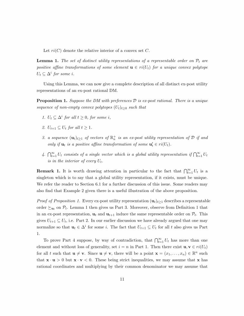
Let ri(C) denote the relative interior of a convex set C.
Lemma 1. The set of distinct utility representations of a representable order on Pt arepositive affine transformations of some element u ∈ ri(Ut) for a unique convex polytopeUt ⊆ ∆i for some i.
Using this Lemma, we can now give a complete description of all distinct ex-post utilityrepresentations of an ex-post rational DM.
Proposition 1. Suppose the DM with preferences D is ex-post rational. There is a uniquesequence of non-empty convex polytopes (Ut)t≥0 such that
1. Ut ⊆ ∆i for all t ≥ 0, for some i,
2. Ut+1 ⊆ Ut for all t ≥ 1.
3. a sequence (ut)t≥1 of vectors of R+n is an ex-post utility representation of D if and
only if ut is a positive affine transformation of some u′t ∈ ri(Ut).
4.⋂∞t=1 Ut consists of a single vector which is a global utility representation if
⋂∞t=1 Ut
is in the interior of every Ut.
Remark 1. It is worth drawing attention in particular to the fact that⋂∞t=1 Ut is a
singleton which is to say that a global utility representation, if it exists, must be unique.We refer the reader to Section 6.1 for a further discussion of this issue. Some readers mayalso find that Example 2 given there is a useful illustration of the above proposition.
Proof of Proposition 1. Every ex-post utility representation (ut)t≥1 describes a representableorder �ut on Pt. Lemma 1 then gives us Part 3. Moreover, observe from Definition 1 thatin an ex-post representation, ut and ut+1 induce the same representable order on Pt. Thisgives Ut+1 ⊆ Ut, i.e. Part 2. In our earlier discussion we have already argued that one maynormalize so that ut ∈ ∆i for some i. The fact that Ut+1 ⊆ Ut for all t also gives us Part1.
To prove Part 4 suppose, by way of contradiction, that⋂∞t=1 Ut has more than one
element and without loss of generality, set i = n in Part 1. Then there exist u,v ∈ ri(Ut)for all t such that u 6= v. Since u 6= v, there will be a point x = (x1, . . . , xn) ∈ Rn suchthat x · u > 0 but x · v < 0. These being strict inequalities, we may assume that x hasrational coordinates and multiplying by their common denominator we may assume that
11

the coordinates are in fact integers. After that we may change the ith coordinate xi ofx to x′n so as to achieve x1 + x2 + . . . + x′n = 0. Now since un = vn = 0, we will stillhave x′ · u > 0 and x′ · v < 0 for x′ = (x1, x2, . . . , x
′n). Now x′ is uniquely represented
as x′ = µ − ν for two multisets µ and ν. Since the sum of coefficients of x′ was zero, thecardinality of µ will be equal to the cardinality of ν. Let this common cardinality be t.Then, by the above inequalities, we have µ �u ν but µ ≺v ν, which is to say u and v
describe different representable orders on Pt, in contradiction of the fact that u and v,being in ri(Ut), must describe the same representable order on Pt. Since only points inthe relative interior of any Ut are valid utility representations, ∩t≥1Ut cannot be a globalutility representation unless it lies in ri(Ut) for all t.
5 Representation Results
In the previous sections, we have given a set of axioms that describe the behavior of theDM and discussed a class of preferences of the DM that we termed ex-post rational. Wewill now show the following:
Theorem 1 (Main Representation Theorem). Suppose m ≥ 3. The following are equiva-lent:
1. D = (�h)h∈H satisfies Axioms 1– 3.
2. D is ex-post rational.
Remark 2. Taken together with Proposition 1, the above Theorem shows that a D thatsatisfies Axioms 1-3 is uniquely identified by a non-increasing sequence of convex polytopeswhose relative interiors determine the ex-post utility representations.
Remark 3. It is worth noting that Theorem 1 obtains despite the fact that at eachdate there are only finitely many rewards — there are no topological assumptions nordo we rely on the possibility of mixed strategies. The strategy of proof for showing thenon-trivial part of Theorem 1, namely that 1 ⇒ 2, is as follows. We first show thatunder Axioms 1-3, D is equivalent to a partial order over all multisets P that satisfiescertain properties. Ex-post representability of D is then easily seen to be equivalent tothat ordering in P admitting a certain utility representation. We shall therefore provethis latter representation in Section 5.1 and then we will give the proof of Theorem 1 in
12

Section 5.2. Besides being important for the proof of Theorem 1, we expect the materialpresented in Section 5.1 to be of independent interest with applications elsewhere.
Example 2. The requirement in Theorem 1 that there are at least three actions for theagent to choose from cannot be dropped. To see this we have the following counter-examplewithm = 2. Pick any utility vector u = (u1, . . . , un) for the rewards and define D as follows:
Following a history ht ∈ Ht,1. If µ(ai, ht) · u > µ(aj , ht) · u, the DM strictly prefers ai to aj , where i 6= j andi, j = 1, 2.
2. If µ(a1, ht) · u = µ(a2, ht) · u, then(a) If the corresponding multisets of rewards are the same, i.e. µ(a1, ht) = µ(a2, ht),
then the actions are indifferent.(b) Otherwise a1 is strictly preferred.
It may be readily verified that D described above satisfies Axioms 1-3 but does not admitan ex-post utility representation.
5.1 A representation result for orders on multisets
As we know from Section 2, multisets of cardinality t are important for a DM as they areclosely related to histories at date t. The DM has to be able to compare them for all t.At the same time in the context of this paper it does not make much sense to comparemultisets of different cardinalities (it would if we had missing observations). Due to this,our main focus in this subsection is a family of orders (�t)t≥1, where �t is an order onPt. In this case we denote by � the naturally induced partial (but reflexive and transitive)binary relation on P whereby for any µ, ν ∈ P, µ � ν if both µ and ν are of the samecardinality, say t, and µ �t ν and � is undefined otherwise.9
A typical � involves a comparison of only multisets of equal cardinality. Let us considerthe following condition that relates orders of different cardinalities.
Definition 4 (Consistency). An order �= (�t)t≥1 on P is said to be consistent if for anyµ, ν ∈ Pt and any ξ ∈ Ps,
9Mathematically speaking P here is considered as an object graded by positive integers. In a gradedobject all operations and relations are defined on its homogeneous components only.
13

µ �t ν ⇐⇒ µ ∪ ξ �t+s ν ∪ ξ. (5)
One simple example of a non-trivial consistent order is to fix a vector of (not all equal)utility weights u = (u1, . . . , un) and take �t to be the representable order �u on Pt. Alarger class of consistent orders are those that satisfy the following condition.
Definition 5 (Local Representability). An order �:= (�t)t≥1 on P is locally representableif, for every t ≥ 1, there exist ut ∈ Rn such that
µ �s ν ⇐⇒ µ · ut ≥ ν · ut ∀µ, ν ∈ Ps, ∀s ≤ t. (6)
A sequence (ut)t≥1 is said to locally represent � if (6) holds. The order � is said to beglobally representable if there exist u ∈ Rn such that (6) is satisfied for ut = u for all t.
The lexicographic ordering of all multisets is locally representable but not globally.It is easy to check that any locally representable linear order on P is consistent. Moreinterestingly, we have the following:
Proposition 2. An order �= (�t)t≥1 on P is consistent if and only if it is locally repre-sentable.
Remark 4. By the above Proposition, every �t in a consistent order � on P is repre-sentable. Applying Lemma 1 and repeating the proof of Proposition 1 virtually ad verbatim,we note that any consistent order (�t)t≥1 is uniquely identified by a sequence of polytopes(Ut)t≥0 that satisfies the properties listed in Proposition 1.
Proof of Proposition 2. The “if” part is straightforward to verify. Suppose the sequenceof vectors (ut)t≥1 represents �= (�t)t≥1. Let µ, ν ∈ Ps with µ �s ν and η ∈ Pt. Thenµ ·us+t ≥ ν ·us+t since us+t can be used to compare multisets of cardinality t as t < t+ s.But now
(µ+ η) · us+t − (ν + η) · us+t = µ · us+t − ν · us+t ≥ 0
which means µ+ η �s+t ν + η.To see the converse, let �= (�t)t≥1 be consistent. An immediate implication of consis-
tency is that for any µ1, ν1 ∈ Pt and µ2, ν2 ∈ Ps,
µ1 �t ν1 and µ2 �s ν2 =⇒ µ1 ∪ µ2 �t+s ν1 ∪ µ2 �t+s ν1 ∪ ν2, (7)
14

where we have µ1 ∪ µ2 �t+s ν1 ∪ ν2 if and only if either µ1 �t ν1 or µ2 �s ν2.Now suppose, by way of contradiction, that local representability fails at some t which
means that ut is the first vector that cannot be found. Note that there are N =(n+t−1
t
)multisets of cardinality t in total. Let us enumerate all the multisets in Pt so that
µ1 �t µ2 �t · · · �t µN−1 �t µN . (8)
Some of these relations may be equivalencies, the others will be strict inequalities. LetI = {i | µi ∼t µi+1} and J = {j | µj �t µj+1}. If �t is complete indifference, i.e. allinequalities in (8) are equalities, then it is representable and can be obtained by assigning1 to all of the utilities. Hence at least one ranking in (8) is strict or J 6= ∅.
The non-representability of �t is equivalent to the assertion that the system of linearequalities (µi − µi+1) · x = 0, i ∈ I, and linear inequalities (µj − µj+1) · x > 0, j ∈ J , hasno semi-positive solution.
A standard linear-algebraic argument tells us that inconsistency of the system above isequivalent to the existence of a nontrivial linear combination
N−1∑i=1
ci(µi − µi+1) = 0 (9)
with non-negative coefficients cj for j ∈ J of which at least one is non-zero (see, for example,Theorem 2.9 of Gale (1960), page 48). Coefficients ci, for i ∈ I, can be replaced by theirnegatives since the equation (µi − µi+1) · x = 0 can be replaced with (µi+1 − µi) · x = 0.Thus we may assume that all coefficients of (9) are non-negative with at least one positivecoefficient cj for j ∈ J . Since the coefficients of vectors µi − µi+1 are integers, we maychoose c1, . . . , cn to be non-negative rational numbers and ultimately non-negative integers.
The equation (9) can be rewritten as
N−1∑i=1
ciµi =N−1∑i=1
ciµi+1, (10)
which can be rewritten as the equality of two unions of multisets:
N−1⋃i=1
µi ∪ . . . ∪ µi︸ ︷︷ ︸ci
=N−1⋃i=1
µi+1 ∪ . . . ∪ µi+1︸ ︷︷ ︸ci
(11)
15

which contradicts to cj > 0, µj � µj+1 and (7). This contradiction proves the proposition.
5.2 Proof of Theorem 1
Proof of Theorem 1. Let us show the non-trivial part of the theorem, which is, 1⇒ 2. Webegin by defining, for each t ≥ 1, a binary relation �∗t on Pt as follows: for any µ, ν ∈ Pt,
µ �∗t ν or µ �∗t ν ⇐⇒ there exists a, b ∈ A and a history ht ∈ Ht
such that µ = µ(a, ht) and ν = µ(b, ht) and (12)
a �ht b or a �ht b respectively.
We need to show that �∗t is antisymmetric. Otherwise, for a certain pair of multisetsµ, ν ∈ Pt, different choices of histories and actions can result in both µ �∗t ν and ν �∗t µat once. However, we claim that:
Claim 1. For any a, b, c, d ∈ A and any two histories ht, h′t ∈ Ht such that µ(a, ht) =µ(c, h′t) and µ(b, ht) = µ(d, h′t),
a �ht b ⇐⇒ c �ht′ d.
The above claim ensures that �∗t is antisymmetric since �h is antisymmetric. It isnow also clear that the sequence �∗= (�∗t )t≥1 inherits the non-triviality assumption in thesense that for some t the relation �∗t is not a complete indifference. Next we claim that
Claim 2. �∗t is a preference ordering on Pt.
Both of the above claims only rely on Axiom 1 and Axiom 2. By a repeated applicationof Axiom 3, we see at once that
Claim 3. The sequence �∗= (�∗t )t≥1 is a consistent order on P (in the sense of Defini-tion 4).
Applying Proposition 2 we note that (�∗t )t≥1 is locally representable. Any (ut)t≥1
representation of (�∗t )t≥1 then, by construction of the latter, will constitute an ex-postutility representation of D.
16

The proof of Theorem 1 is therefore complete upon giving the proofs of Claim 1 andClaim 2 and verifying that fact that 2⇒ 1. All of these are relatively straightforward butnevertheless relegated to the Appendix.
6 Discussion
In this section, we shall discuss several aspects our model including the empirical implica-tions and robustness of Theorem 1. Let L(n) in Rn denote the linear hyperplane whosenormal is n, i.e.
L(n) = {x ∈ Rn : n · x = 0}. (13)
6.1 On the set of all utility representations
Theorem 1 shows that a utility representation obtains under fairly weak assumptions.The set of feasible utility assignments were given in Proposition 1. Note that since autility assignment u ∈ Ut is already normalised, no two elements of ri(Ut) are affinetransformations of each other (see the proof of Lemma 1). In this sense, the DM may beambiguous about the actual value she assigns to individual rewards although the relativeranking of the rewards remains unchanged over time. The following example illustrateshow the possible utility assignments to the rewards, i.e. the polytopes in Proposition 1,evolve.
Example 3. Assume there are three rewards, i.e. R = {1, 2, 3}. Recall from the proofof Theorem 1 that a D that satisfies Axioms 1-3 is equivalent to a consistent orderingover P as given in Definition 4 and an ex-post utility representation of D is a local utilityrepresentation of � as given in Definition 5. Let �= (�t)t≥1 be that ordering over P.
Since P1 = R, the order �1 is simply a ranking of the three rewards. Let us assumethat 1 �1 2 �1 3. Then any choice of utilities for the rewards u1 > u2 > u3 would represent�1 on P1. One can normalise these by setting the least utility to zero and scaling them toadd to one so that vectors from the relative interior of
U1 = {(u1, 1− u1, 0) | u1 ∈ [1/2, 1]}
effectively give us all representations of �1.
17

Next, we consider P2. The multisets in P2 are listed in the table below with multiplic-ities for each multiset appearing in the first three columns. In the rightmost column wegive the notation for each multiset.
1 2 3 Notation
µ1 2 0 0 12
µ2 1 1 0 12µ3 1 0 1 13
1 2 3 Notation
µ4 0 2 0 22
µ5 0 1 1 23µ6 0 0 2 32
Table 1: P2 = {µ1, µ2, µ3, µ4, µ5, µ6}.
Consistency requires that �2 must necessarily rank 12 �2 12 as the top two multisetsand 23 �2 32 as two bottom ones, Furthermore, 13 and 22 must be placed in between12 and 23 although we have freedom to choose the relation between them. Thus, wehave three possible orderings of P2 that would be consistent with the given �1 dependingon how this ambiguity is resolved. If 13 ∼2 22, representability gives u1 = 2u2, whichimmediately pins down U2 = {(2/3, 1/3, 0)}. Moreover, for all t > 2 we will also haveUt = U2 = {(2/3, 1/3, 0)}.
U1 [12 , 1]
uulllllllllllllllll
�� ))RRRRRRRRRRRRRRRRR
U2 [12 ,23 ]
||yyyy
yyyy
�� ""FFFF
FFFF
{23}
��
[23 , 1]
||yyyy
yyyy
�� ""EEEE
EEEE
U3 [12 ,35 ] {3
5} [35 ,23 ] {2
3} [23 ,34 ] {3
4} [34 , 1]
Figure 1: Schematic description of consistent orders on Pt[3], t ≤ 3, when 1 �1 2 �1 3.
If, on the other hand, 13 �2 22, we have U2 = {(u1, 1− u1, 0) |u1 ∈ [2/3, 1]} and in theresidual case of 22 �2 13, we have U2 = {(u1, 1 − u1, 0) |u1 ∈ [1/2, 2/3]}. Going furtherto P3 = P3[3], the possibilities are listed in Figure 3. In the figure, the set Ut is encodedby the interval of values that u1 is allowed to take. For a u1 that lies in the different setslisted in the terminal nodes of the graph, we obtain a distinct preference relation on P3
that is consistent with 1 �1 2 �1 3. The above process can be continued for t > 3 alongsimilar lines.
18

As illustrated in the above example, the DM becomes increasingly precise over thevalues assigned to the rewards. This is also true in general as Ut+1 ⊆ Ut. However, thelimiting set ∩t≥1Ut may not constitute a representation as shown in the following example.
Example 4. Consider the case where there are three rewards, i.e. R = {1, 2, 3} andD = (�h)h∈H is the lexicographic ordering, where
a �h b ⇔
if µ1(a, h) > µ1(b, h)
if µ1(a, h) = µ1(b, h) and µ2(a, h) > µ2(b, h).(14)
This ordering is represented by choosing Ut whose elements are of the form (u1, u2, u3) =(u1, 1−u1, 0) where u1 ∈ (t/(t+ 1), 1). And yet, there cannot be a global representation ofthis lexicographic ordering since the intersection
⋂∞t=1 Ut = (1, 0, 00) is a boundary point.
Recall that although a global utility representation may not exist but if one does, itmust be unique. (See Proposition 2.)
To ensure the existence of a global utility representation, one requires some form of theArchimedean axiom on the DM’s behavior. We do not pursue this here since the role ofsuch axioms is well understood in Decision Theory.
6.2 Random Rewards and Observed Behavior
For the rest of this section, suppose that there is a stationary stochastic process Xt thatgenerates the rewards. From the probability measure that governs this process, one cancompute the probability that an action ai receives the reward j at any given date. Denotethis probability by qij . To each action a1, . . . , am, we then have a corresponding lotteryqi = (qi1, . . . , qin) over the set of rewards.
Consider, for the moment, a DM that is fully aware of the environment and satisfies theexpected utility hypothesis. Given vNM utility vector for the rewards u = (u1, . . . , un),naturally we shall say that an action ai∗ is a best action for the DM if
u · qi∗ ≥ u · qi for all 1 ≤ i ≤ m. (15)
Our interest here is in the observed behavior in the above environment of a DM whodoes not know the environment but satisfies Axioms 1-3 vis-a-vis a DM that knows theenvironment. We will show the following.
19

Theorem 2. Consider a DM that is consistent with Axioms 1-3 and admits a global utilityrepresentation u. Suppose the stationary stochastic process Xt is such that there is a uniquebest action. Then, with probability one, the DM chooses the best action corresponding to u
at all but finitely many dates.
Remark 5. The best action is determined by a finite set of linear inequalities (15). Fora generic choice of probabilities and global utility vectors, the existence of a unique bestaction is therefore assured. Thus, the existence of a unique best action in Theorem 2 is aweak requirement.
To see how Theorem 2 obtains, pick any two actions, say a1 and a2. Suppose that ourstationary stochastic process produces reward ri for a1 and reward rj for a2 with probabilitypij . We model this event by the vector fij = ei − ej . So without loss of generality we mayassume that the stochastic process Xt actually produces not prizes but these vectors andlet Yt = X1 + · · ·+Xt. To illustrate, suppose R = {1, 2, 3} and the following sequences ofprizes are realized
a1: 1 1 2 3 2 2 1 3 3 3 1 2 . . .
a2: 2 3 1 1 3 1 2 2 1 2 3 3 . . .
The initial five realizations of our stochastic process X1, X2, X3, X4 and X5 are respec-tively
f12 =
1−1
0
, f13 =
10−1
, f21 =
−110
, f31 =
−101
, f23 =
01−1
and correspondingly
Y1 =
1−1
0
, Y2 =
2−1−1
, Y3 =
10−1
, Y4 =
000
, Y5 =
01−1
We are interested in the behavior of Yt = X1 + X2 + . . . + Xt. For, by Theorem 1, a
DM with a global utility representation u chooses the first action at moment t if Yt ·u > 0,chooses the second action at moment t if Yt ·u < 0 and chooses any action when Yt ·u = 0.
20

Observe that the coordinates of Yt will necessarily sum to zero. Therefore, Yt lies onthe hyperplane L(1) where 1 = (1, . . . , 1). In fact, Yt is a random walk on the integergrid in L(1) generated by the vectors fij . These vectors are not linearly independent. Forinstance, in the above example, we have f12 + f23 = f13. Thus if we take f12 and f23 as abasis for this grid, then f13 will represent a diagonal move. In general, the m − 1 vectors{f12, f23, . . . , fm−1m} form a basis, so that having m prizes we have a walk on an m − 1dimensional grid with a drift
d =∑i 6=j
pijfij .
We are now ready to prove the theorem:
Proof of Theorem 2. Consider the hyperplane L = L(u). With no loss in generality, labelthe unique best action as a1 and pick any other action and label it a2. It suffices to showthat with probability one, the DM chooses a1 in all but finitely many periods. Axiom 1will then complete the proof.
First, note that10
q1 − q2 = d. (16)
By hypothesis then, u · d > 0 which is to say that d lies above the hyperplane L. By theStrong Law of Large numbers, 1
tYt converges almost surely to d. Hence, with probabilityone, Yt also lies above L for all but finitely many t. Recalling that the DM may choose a2
only when Yt · u ≤ 0, the claim follows readily upon appealing to Axiom 1.
6.3 Empirical Test of the Axioms
In this section, our interest is in what an external observer can infer about a DM, who isconsistent with Axiom 1-3, simply by observing her sequential choices and the sequence ofrewards.
To first illustrate and simplify exposition, assume that there are only two actions andR = {1, 2, 3}. Suppose the following sequence of rewards are realised:
10To see (16), note that q1i =∑n
j=1 pij and q2i =∑n
j=1 pji. Next, observe that the `th coordinate ofany fij is non-zero only if ` is either i or j. Therefore, diei =
∑nj=1 pijfij +
∑nj=1 pjifji or that diei =(∑n
j=1(pij − pji))ei.
21

a1: 1 1 2 3 2 2 1 3 3 3 1 2a2: 2 3 1 1 3 1 2 2 1 2 3 3
By observing the choices of the DM along this sequence, the DM’s preferences over theactions following all two period histories (i.e. �h2 for h2 ∈ H2) will be revealed. Indeed,to discover this relation, all we need to do is figure out how she ranks the six multisetsin P2 listed in Table 3. The comparisons 12 ? 22, 22 ? 32 and 12 ? 32 will be encounteredat moments 1,5 and 9. The comparisons 12 ? 23, 13 ? 22 and 12 ? 32 will be encountered atmoments 4,8 and 12, respectively. When the DM resolves these comparisons by choosingone action or another the whole preference order on P2 will be revealed. On the otherhand, if 2 is the least valued prize, the sequences
a1: 1 3 1 3 1 3 . . .
a2: 2 2 2 2 2 2 . . .
never reveals agent’s preferences between rewards 1 and 3.More generally, one can design particular sequences of rewards and by observing those
rewards, one can figure out what �ht is for all ht ∈ Ht. This amounts to constructing asequence of rewards that reveals the implied preferences on Pt[n]. The idea is, at everystep, to undo all the previous comparisons and then to present the agent with the new one.Also note that for such revelation to occur the DM must switch from one action to another.Such sequences and switching can be engineered via experiments in a laboratory. However,if rewards are instead drawn at random, we know from Theorem 2 and Remark 5, the DMrarely switches.11
The point is, that while it is feasible to discover a DM’s characteristics using experi-mental data from the laboratory, typically only very limited conclusions can be drawn of aDM using the empirical data on her choices out in the field (where the rewards are drawnat random). We emphasise however, that the inability to deduce the preference relationdoes undermine the refutability of our Axioms.
Proposition 3. Suppose we observe that a DM, who is known to have non-trivial pref-erences, has chosen actions a1, . . . , at, . . . , aT in successive periods and the history hT .Suppose that any u = (u1, . . . , un) that satisfies the system of inequalities
µ(at, ht) · u ≥ µ(a, ht) · u a ∈ A, t = 1, . . . , T, (17)11 Should the non-generic possibility of a driftless {Yt} occur (the random process described Section 6.2)
with n = 3 rewards, the walk will be recurrent and the utilities will still be revealed. Not so for n > 3.
22

where ht is the sub-history of hT until period t, is necessarily of the form ui = uj for alli, j = 1, . . . , n. Then the DM violates one of the Axioms 1-3.
Proof. Suppose that, by way of contradiction, the DM obeys Axioms 1-3. By Theorem 1,the DM is then ex-post rational. Applying Proposition 1 and choosing any ex-post utilityrepresentation (ut)t≥1 of such a DM, we note that uT ∈ UT must be a solution to theabove system of inequalities. Furthermore, since UT lies on a facet of the unit simplex∆ ⊂ Rn, uT is in fact a solution of (17) such that not all of its coordinates are equal. Thiscontradiction establishes the Proposition.
6.4 Ex-post Rationality with Bounded Recall
Throughout, we had assumed that the DM can track the entire history. An alternativehypothesis is that she can only track the last k observations. In fact such a hypothesismay be more plausible if the underlying process Xt which produces rewards for actionsis not stationary. Indeed, if Xt becomes uncorrelated after time k, then, even if the DMremembers old observations, they become of no use. A DM who understands this aspectof the environment (but still possibly ignorant about other aspects) may use only the lastk observations.
With bounded recall then, the DM is only required to rank in a consistent fashionmultisets of cardinality not greater than k. But then, Proposition 2 breaks down.
The following is a consistent linear order on P3[4] (taken from Sertel and Slinko (2005))but is not representable.
13 � 122 � 123 � 124 � 122 � 123 � 124 � 132 � 134 � 23 �
223 � 142 � 224 � 232 � 234 � 242 � 33 � 324 � 342 � 43.
Indeed we have:223 � 142, 242 � 33, 134 � 23. (18)
If this ranking were representable then the respective system of inequalities
2u2 + u3 ≥ u1
u2 ≥ 3u3
u1 + u3 ≥ 3u2
23

would have a non-zero non-negative solution, but it has not. These inequalities implyu1 = u2 = u3 = u4 = 0.
Whether some weaker form of representability of the DM can be achieved remains atopic for future research.
7 Related Literature
There is a large body of literature that begins with the assumption that the DM is a longrun expected utility maximiser. Certain simple thumb rules are posited and the questionis if these simple rules yield the optimizing behavior of a fully rational player. See Lettauand Uhlig (1995), Schlag (1998) and Robson (2001) among others. Given the Axioms andthe representation, the analysis presented in Section 6.2 is in this spirit.
The main focus of this paper is however on the axiomatic development of the DM’sbehavior that attempts to capture from first principles how a DM learns. From this stand-point, Borgers, Morales, and Sarin (2004) and ER are two works that share this concern.The former considers behavioral rules that take the action/payoff pair that was realised inthe previous period and map it to a mixed strategy on A. The desirable properties thatare imposed on a behavioral rule (monotonicity, expediency, unbiasedness etc.) involvecomparing the payoffs realised in the previous periods. Thus, no distinction is being madebetween payoffs and rewards.
ER is the closest relative of this work as it explicitly considers axioms on sequencesof preferences in a dynamic context. Like us, ER study a family of preference relations{�ht}t≥1 on the set of actions A indexed by histories. There are however both formaland conceptual differences. Unlike us, they find it necessary to extend �ht to a preferencerelation over ∆(A), the set of all lotteries over A while in our paper we do not needlotteries. They too, just as in Borgers, Morales, and Sarin (2004), assume that the rewardsare monetary payoffs. In our setting the outcome of an action is an arbitrary reward. Thisdistinction is important since, as we have seen, at each stage, there is in fact a convexpolytope of endogenously determined utilities for the rewards that determines the DM’sbehavior. Interestingly, our representation result Theorem 1 shows that our three axiomsenough to at once jointly determine the updating method and the payoffs to underlyingrewards.
Conceptually, ER’s focus is on the transition from the preference relation �ht to �ht+1
in response to the most recently observed rewards. A driving assumption in their work is
24
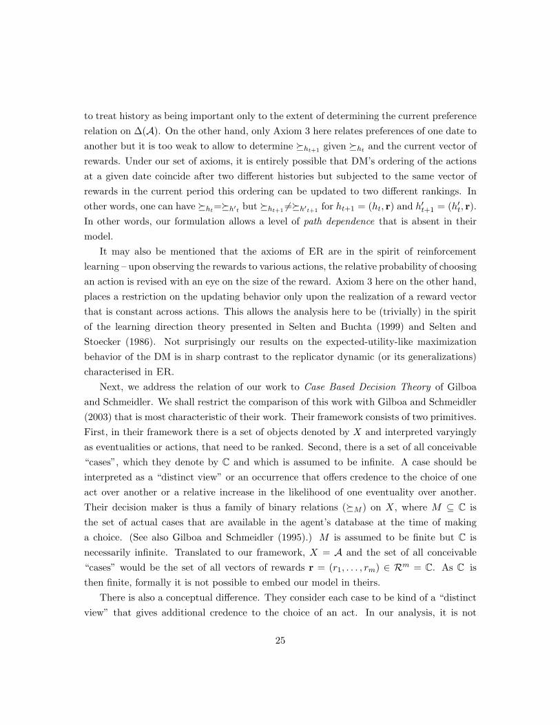
to treat history as being important only to the extent of determining the current preferencerelation on ∆(A). On the other hand, only Axiom 3 here relates preferences of one date toanother but it is too weak to allow to determine �ht+1 given �ht and the current vector ofrewards. Under our set of axioms, it is entirely possible that DM’s ordering of the actionsat a given date coincide after two different histories but subjected to the same vector ofrewards in the current period this ordering can be updated to two different rankings. Inother words, one can have �ht=�h′t but �ht+1 6=�h′t+1 for ht+1 = (ht, r) and h′t+1 = (h′t, r).In other words, our formulation allows a level of path dependence that is absent in theirmodel.
It may also be mentioned that the axioms of ER are in the spirit of reinforcementlearning – upon observing the rewards to various actions, the relative probability of choosingan action is revised with an eye on the size of the reward. Axiom 3 here on the other hand,places a restriction on the updating behavior only upon the realization of a reward vectorthat is constant across actions. This allows the analysis here to be (trivially) in the spiritof the learning direction theory presented in Selten and Buchta (1999) and Selten andStoecker (1986). Not surprisingly our results on the expected-utility-like maximizationbehavior of the DM is in sharp contrast to the replicator dynamic (or its generalizations)characterised in ER.
Next, we address the relation of our work to Case Based Decision Theory of Gilboaand Schmeidler. We shall restrict the comparison of this work with Gilboa and Schmeidler(2003) that is most characteristic of their work. Their framework consists of two primitives.First, in their framework there is a set of objects denoted by X and interpreted varyinglyas eventualities or actions, that need to be ranked. Second, there is a set of all conceivable“cases”, which they denote by C and which is assumed to be infinite. A case should beinterpreted as a “distinct view” or an occurrence that offers credence to the choice of oneact over another or a relative increase in the likelihood of one eventuality over another.Their decision maker is thus a family of binary relations (�M ) on X, where M ⊆ C isthe set of actual cases that are available in the agent’s database at the time of makinga choice. (See also Gilboa and Schmeidler (1995).) M is assumed to be finite but C isnecessarily infinite. Translated to our framework, X = A and the set of all conceivable“cases” would be the set of all vectors of rewards r = (r1, . . . , rm) ∈ Rm = C. As C isthen finite, formally it is not possible to embed our model in theirs.
There is also a conceptual difference. They consider each case to be kind of a “distinctview” that gives additional credence to the choice of an act. In our analysis, it is not
25

just the set of “distinct views” but also “how many” times any of those given views areexpressed is important. To elaborate further, Gilboa and Schmeidler (2003) work witha family of relations �M⊆ X × X with M a finite set of C being the parameter. C isnecessarily infinite. We, on the other hand, work with a family of relations �µ⊆ X × Xwhere the parameter µ is a multiset of C (a finite set).
8 Conclusion and Future Work
In this paper, we have presented a theory of choice in a complex environment, a theory thatdoes not rely on the action/state/consequence approach. Three simple axioms secure thatthe DM has an ex-post utility representation and behaves as an expected utility maximiserwith regard to the empirical distribution of rewards.
In future work we expect to relax the following assumptions:
(a) that the agent is learning in a social setting. A history in this case would containmissing observations,
(b) allow the DM to have bounded recall,
(c) allow for the possibility that the DM faces a possibly different problem in each period(thus making the analysis comparable to case based decision theory of Gilboa andSchmeidler (1995)).
Appendix
Proof of Lemma 1. We recall a few basic facts about hyperplane arrangements in Rn (seeOrlik and Terao (1992) for more information about them). A hyperplane arrangement Ais any finite set of hyperplanes. Given a hyperplane arrangement A and a hyperplane J ,both in Rn, the set
AJ = {L ∩ J | L ∈ A}
is called the induced arrangement of hyperplanes in J .A region of an arrangement A is a connected component of the complement U of the
union of the hyperplanes of A, i.e., of the set
U = Rn \⋃L∈A
L.
26

Any region of an arrangement is an open set.Every point u = (u1, . . . , un) ∈ Rn defines an order �u on Pt, which obtains when we
allocate utilities u1, . . . , un to prizes i = 1, 2, . . . , n, that is
µ �u ν ⇐⇒n∑i=1
µ(i)ui ≥n∑i=1
ν(i)ui. (19)
Any order on Pt that can be expressed as above for some u ∈ Rn is said to be repre-sentable. We will now argue that the representable linear orders on Pt are in one-to-onecorrespondence with the regions of the following hyperplane arrangement.
Consider the hyperplane arrangement
A(t, n) ={L(µ− ν) | µ, ν ∈ Pt[n]
}. (20)
where L(µ− ν) is as given by Eq. (13).The set of representable linear orders on Pt[n] is in one-to-one correspondence with the
regions of A = A(t, n). In fact, then the linear orders �u and �v on Pt will coincide if andonly if u and v are in the same region of the hyperplane arrangement A. This immediatelyfollows from the fact that the order µ �x ν changes to µ ≺x ν (or the other way around)when x crosses the hyperplane L(µ − ν). The closure of every such region is a convexpolytope.
Let us note that in (19) we can divide all utilities by u1 + . . . + un and the inequalitywill still hold. Hence we could from the very beginning consider that all vectors of utilitiesare in the hyperplane J given by x1 + . . . + xn = 1 and even in the simplex ∆ given byxi ≥ 0 for i = 1, 2, . . . , n.
Thus, every representable linear order on Pt is associated with one of the regions of theinduced hyperplane arrangement AJ .
Let us note that due to our non-triviality assumption the vector(
1n , . . . ,
1n
)does not
correspond to any order. Consider a utility vector u ∈ ∆ different from(
1n , . . . ,
1n
)lying
in one of the regions of AJ whose closure is V . We then can normalise u applying apositive affine linear transformation which makes its lowest utility zero. Indeed, supposethat without loss of generality u1 ≥ u2 ≥ . . . ≥ un 6= 1
n . Then we can solve for α and β thesystem of linear equations α+ nβ = 1 and αun + β = 0 and since the determinant of thissystem is 1 − nun 6= 0 its solution is unique. Then the vector of utilities u′ = αu + β · 1will lie on the facet ∆n of ∆ and we will have �u′=�u. Hence the polytope V has one face
27

on the boundary of ∆. We denote it U . So if the order � on Pt is linear the dimension ofU will be n− 2.
In general, when the order on Pt is not linear, the utility vector u that represents thisorder must be a solution to the finite system of equations and strict inequalities:
(µ− ν) · u = 0 whenever µ ∼u ν,
(µ− ν) · u > 0 whenever µ �u ν,∀µ, ν ∈ Pt. (21)
Then u will lie in one (or several) of the hyperplanes of A(k, n). In that hyperplane anarrangement of hyperplanes of smaller dimension will be induced by A(k, n) and u willbelong to a relative interior of a polytope U of dimension smaller than n− 2.
Let now �= (�t)t≥1 be a consistent order on P. By Proposition 1 it is locally repre-sentable. We have just seen that in such case, for any t, there is a convex polytope Ut suchthat any vector ut ∈ ri(Ut) represents �t. Due to consistency any vector us ∈ ri(Us), fors > t will also represent �t so Ut ⊇ Us. Thus we see that our polytopes are nested. Notethat only points in the relative interior of Ut are suitable points of utilities to rationalise �t.We also note that the intersection
⋂∞t=1 Ut has exactly one element. This is immediately
implied by the following
Proof of Theorem 1. We give the proofs of Claim 1, Claim 2 and the fact that 2 ⇒ 1 insequence.
Proof of Claim 1. Take the hypothesis as given. If the actions a, b, c, d ∈ A are distinct,consider a history gt ∈ Ht such that gt(a) = ht(a), gt(b) = ht(b), gt(c) = h′t(a) andgt(d) = h′t(b). Applying Axiom 2, a ∼gt c and b ∼gt d and therefore, a �gt b ⇔ c �gt d.Apply Axiom 1 to complete the claim.
Suppose now that a, b, c, d are not all distinct. We will prove that if µ(a, h) = µ(c, h′)and µ(b, h) = µ(b, h′), then
a �ht b⇐⇒ c �h′t b,
which is the main case. Let us consider five histories presented in the following table:
h h1 h2 h3 h′
a h(a) h(a) h′(b) h′(b) h′(a)
b h(b) h(b) h(b) h′(b) h′(b)
c h(c) h′(c) h′(c) h′(c) h′(c)
28

In what follows we repeatedly use Axiom 1 and Axiom 2 and transitivity of �hi , i = 1, 2, 3.Comparing the first two histories, we deduce that c ∼h1 a �h1 b and c �h1 b. Nowcomparing h1 and h2 we have c �h2 b ∼h2 a and c �h2 a. Next, we compare h2 and h3
and it follows that c �h3 a ∼h2 b, whence c �h3 b. Now comparing the last two historieswe obtain c �h′ b, as required.
Proof of Claim 2. Given the fact that actions must be ranked for all conceivablehistories, �∗t is a complete ordering of Pt. From its construction, �∗t is also is reflexive.Again, through appealing to Axiom 1 and Axiom 2 repeatedly, it may be verified that it isalso transitive. Indeed, choose µ, ν, ξ ∈ Pt such that µ �∗t ν and ν �∗t ξ. Pick three distinctactions a, b, c ∈ A and consider a history ht ∈ Ht such that µ(a, ht) = µ, µ(b, ht) = ν andµ(c, ht) = ξ. By definition, a �ht b and b �ht c while transitivity of �ht shows that a �ht c.Hence µ �∗t ξ.
Finally, we turn to the implication 2⇒ 1. That Axioms 1 and 2 are met by an ex-postrational D is easy to see. To prove that Axiom 3 holds, suppose that the sequence of utilityvectors (ut)t≥1 represents the DM and suppose a �ht b and at the moment t both actions aand b yield a reward i. Then we have µ(a, ht+1) = µ(a, ht)+ei and µ(b, ht+1 = µ(b, ht)+ei,where ei is the ith vector of the standard basis of Rn. Due to consistency condition, theutility vector ut+1 can also be used for comparisons of histories shorter than t + 1, so wehave
µ(a, ht) · ut+1 ≥ µ(a, ht) · ut+1
From here we obtain:
µ(a, ht+1) · ut+1 = (µ(a, ht) + ei) · ut+1 ≥ (µ(b, ht) + ei) · ut+1 = µ(b, ht+1) · ut+1.
Hence a �ht+1 b.
References
Anscombe, F., and R. Aumann (1963): “A definition of subjective probabiliy,” Annalsof Mathematical Statistics, 34, 199–205.
29

Aumann, R. J., and J. H. Dreze (2008): “Rational Expectations in Games,” AmericanEconomic Review, 98(1), 72–86.
Blume, L. E., D. A. Easley, and J. Y. Halpern (2006): “Redoing the Foundations ofDecision Theory,” in Tenth International Conference on Principles of Knowledge Rep-resentation and Reasoning KR(2006), pp. 14–24.
Borgers, T., A. J. Morales, and R. Sarin (2004): “Expedient and Monotone LearningRules,” Econometrica, 72(2), 383–405.
Brown, G. W. (1951): “Iterative solutions of games by fictitious play,” in In ActivityAnalysis of Production and Allocation, ed. by T. C. Koopmans. New York: Wiley.
Dekel, E., B. L. Lipman, and A. Rustichini (2001): “Representing Preferences witha Unique Subjective State Space,” Econometrica, 69(4), 891–934.
Easley, D., and A. Rustichini (1999): “Choice without Beliefs,” Econometrica, 67(5),1157–1184.
Ellsberg, D. (1961): “Risk, Ambiguity, and the Savage Axioms,” Quarterly Journal ofEconomics, 74(4).
Fudenberg, D., and D. K. Levine (1998): The Theory of Learning in Games. MITPress.
Gale, D. (1960): The Theory of Linear Economic Models. McGraw-Hill, New-York.
Gigerenzer, G., and R. Selten (eds.) (2001): Bounded Rationality: The AdaptiveToolbox. MIT Press.
Gilboa, I., and D. Schmeidler (1995): “Case-Based Decision Theory,” The QuarterlyJournal of Economics, 110(3), 605–39.
(2001): A Theory of Case-Based Decisions. Cambridge University Press.
(2003): “Inductive Inference: An Axiomatic Approach,” Econometrica, 71(1),1–26.
Hopkins, E. (2002): “Two Competing Models of How People Learn in Games,” Econo-metrica, 70(6), 2141–2166.
30

Karni, E. (2006): “Subjective expected utility theory without states of the world,” Jour-nal of Mathematical Economics, 42(3), 325–342.
Knight, F. H. (1921): Risk, Uncertainty and Profit. Boston, MA: Hart, Schaffner &Marx; Houghton Mifflin Co.
Lettau, M., and H. Uhlig (1995): “Rules of Thumb and Dynamic Programming,”Tilburg University Discussion Paper.
Orlik, P., and H. Terao (1992): Arrangements of Hyperplanes. Springer-Verlag, Berlin.
Robson, A. J. (2001): “Why Would Nature Give Individuals Utility Functions?,” Journalof Political Economy, 109, 900–914.
Savage, L. J. (1954): The Foundations of Statistics. Harvard University Press, Cam-bridge, Mass.
Schlag, K. H. (1998): “Why Imitate, and If So, How?, : A Boundedly Rational Approachto Multi-armed Bandits,” Journal of Economic Theory, 78(1), 130–156.
Selten, R. (2001): “What is bounded rationality?,” in Bounded Rationality: The AdaptiveToolbox, ed. by G. Gigerenzer, and R. Selten. MIT Press.
Selten, R., and J. Buchta (1999): “Experimental Sealed-Bid First Price Auctions withDirectly Observed Bid Functions.,” In D. Budescu, I. Erev, and R. Zwick (eds.), Gamesand Human Behavior: Essays in the Honor of Amnon Rapoport NJ: Lawrenz AssociatesMahwah.
Selten, R., and R. Stoecker (1986): “End Behavior in Sequences of Finite Prisoners’Dilemma Supergames: A Learning Theory Approach,” Journal of Economic Behaviorand Organization., 7, 47–70.
Sertel, M. R., and A. Slinko (2005): “Ranking Committees, Income Streams or Mul-tisets,” Economic Theory.
31