On Customized Goods, Standard Goods, and Competition¶

Niladri B. Syam C. T. Bauer College of Business

University of Houston 385 Melcher Hall, Houston, TX 77204

Email: nbsyam@uh.edu Phone: (713) 743 4568 Fax: (713) 743 4572

Nanda Kumar School of Management

The University of Texas at Dallas Email: nkumar@utdallas.edu

Phone: (972) 883 6426 Fax: (972) 883 6727

Forthcoming: Marketing Science

November 10, 2005

¶ Authors are listed in reverse alphabetic order; both authors contributed equally to the article. The authors wish to thank the Editor-in-Chief Steve Shugan, the AE and two anonymous reviewers for their valuable comments. We also wish to thank Professors Preyas Desai, Jim Hess, Chakravarthi Narasimhan, Surendra Rajiv, Ram Rao and the seminar participants at the Carlson School of Management (Minnesota), Wash U. (St. Louis), Singapore Management University and National University of Singapore for many insightful comments. The usual disclaimer applies.

On Customized Goods, Standard Goods, and Competition

Abstract

In this study, we examine firms’ incentive to offer customized products in addition to their standard products in a competitive environment. We offer several key insights. First, we delineate market conditions in which firms will (will not) offer customized products in addition to their standard products. Surprisingly, we find that when firms offer customized products they can not only expand demand but can also increase the prices of their standard products relative to when they do not. Second, we find that when a firm offers customized products it is a dominant strategy for it to also offer its standard product. This result highlights the role of standard products and the importance of retaining them when firms offer customized products. Third, we identify market conditions under which ex-ante symmetric firms will adopt symmetric or asymmetric customization strategies. Fourth, we highlight how the degree of customization offered in equilibrium is affected by market parameters. We find that the degree of customization is lower when both firms offer customized products relative to the case when only one firm offers customized products. Finally, we show that customizing products under competition does not lead to a Prisoner’s Dilemma.

Key Words: Degree of product customization, mass-customization, standard products, competition, game-theory.

1. Introduction

Advances in information technology facilitate the tracking of consumer behavior

and preferences and allows firms to customize their marketing mix. The practice of firms

customizing their products is pervasive. Product categories that have seen a rise in

customization include apparel, automobiles, cosmetics, furniture, personal computers,

and sneakers among others. The business press has also accorded a lot of importance to

this phenomenon (see for example, The Wall Street Journal, Sept. 7; Sept. 8; and Oct. 8,

2004).

Extant work on product customization in the Information Systems literature

(e.g., Dewan, Jing and Seidmann, 2003) has focused on markets where firms customize

products completely to match the consumers’ preferences. In these models the level of

customization is not a decision variable however, prices of the products are customized.

While the idea of customizing prices and products is very appealing, it is a common

marketing practice, particularly in spatially differentiated product markets, to charge the

same (posted) price for the customized products even if different consumers choose

different options while customizing. For example, at LandsEnd.com consumers can

purchase a standard pair of Jeans for $29.95 or a customized pair for $54. A customer

may choose to customize a range of options but regardless of the options chosen the price

of the customized pair of Jeans is $54. The practice of charging the same price for all

customized variants is not limited to the apparel industry. Indeed Reflect.com a

manufacturer of custom-made cosmetics allows consumers to customize the color and

- 1 -

type of finish (glossy or matte) of a lipstick for $17.1 Once again the price of all variants

is the same regardless of the color or type of finish chosen by different consumers.

In addition, as mentioned in a recent article (The Wall Street Journal, October 8,

2004) the decision of what to customize appears to be a critical strategic decision. For

example, Home Depot’s EXPO division allows consumers to customize the color of rugs,

whereas Rug Rats, a Farmville, Va., manufacturer will customize both the colors and

patterns of its rugs. Similarly, in the home furniture market Ethan Allen customizes

furniture, but will not allow customers to use their own fabric. Crate & Barrel, on the

other hand, will upholster furniture from fabric provided by the customer. These

examples and the discussion in the WSJ article illustrate the fact that the level of

customization is an important strategic variable and firms operating in the same industry

adopt different customization strategies. Extant theory on product customization,

however, does not shed much light on how the level of customization offered is affected

by market characteristics or why firms adopt different customization strategies.2 An

additional consideration in offering customized products is the impact they have on the

prices and profitability of the firms’ standard offerings.

With these institutional practices in mind, we address the following research

questions. First, how is the nature of competition between firms, and their profitability,

affected when they offer customized products in addition to their standard products?

Under what market conditions (if any) can firms benefit from offering customized

products in addition to their standard offerings? Second, is it ever profitable for firms to

1 Similarly, at Timberland.com consumers can get a customized pair of boots for $200 regardless of the options chosen. 2 The level of customization is not a decision variable in Dewan, Jing and Siedmann (2003) so their study does not offer any specific predictions on this issue.

- 2 -

offer only customized products to the exclusion of standard products? Third, when it is

optimal to offer customized products, what should the optimal degree of customization

be, and how is it related to market characteristics? Fourth, what effect does the strategy of

offering customized products have on the intensity of competition between firms’

standard products, and on their prices? Finally, we seek to examine whether ex ante

symmetric firms can pursue asymmetric strategies as it relates to product customization.

The motivation for exploring this issue is to understand the strategic forces that may help

explain why competing firms might adopt different customization strategies.

Our work contributes to the scant but growing literature on product customization

(Dewan, Jing and Seidmann 2003; Syam, Ruan and Hess 2004). Dewan, Jing and

Seidmann (2003) consider a duopoly in which the competing firms offer completely

customized products to match the preferences of a set of consumers and so the degree of

customization is not a decision variable in their model. However, they do allow the prices

to be customized. As noted earlier, it is a common marketing practice to charge the same

price for the customized products even if consumers choose different options while

customizing. Furthermore, firms operating in the same market differ in the degree of

customization offered and in many markets products are not completely customized. We

add to extant literature by examining a setup in which prices of all customized offerings

of a firm are the same and the degree of customization is endogenously determined. In

doing so we offer several predictions that are new and distinct from those offered by

Dewan, Jing and Seidmann (2003). First, we identify the role of market parameters on the

degree of customization offered in equilibrium. Second, Dewan, Jing and Seidmann

(2003) find that the standard good prices remain the same independent of firms’ decision

- 3 -

to offer customized products. In contrast, we find that the price of the standard good may

be higher or lower when firms decide to offer customized products relative to the case

when there are no customized offerings. In addition to being a new finding the fact that

under certain market conditions firms are able to increase the price of the standard

offerings by adding customized products to their product line is very counter-intuitive.

Syam, Ruan and Hess (2004) examine a duopoly in which firms compete by offering

only customized products. In their setup the product has two attributes and firms decide

whether and which attribute(s) to customize. Because standard products do not exist in

their model in equilibrium, they are unable to make statements about the effects of firms’

decision to customize, on the competition between, and pricing of, their standard

products. Most importantly, they find that by offering only customized products in

equilibrium, firms are unable to increase their profits relative to the case when they only

offered standard products. An important contribution of the current paper is to show that

firms can increase profits by offering both standard and customized products.

We also see our paper contributing to the growing literature on customizing the

marketing mix (Zhang and Krishnamurthi 2004; Gourville and Soman 2005; Liu, Putler

and Weinberg 2004). There is a rich literature in marketing and economics (Shaffer and

Zhang 1995, Bester and Petrakis 1996, Fudenberg and Tirole 2000, Chen and Iyer 2002,

Villas-Boas 2003) which examines the effect of customizing prices to individual

customers. In general the finding is that customized pricing among symmetric firms tends

to intensify competition as a firm’s promotional efforts are simply neutralized by its rival.

We contribute to this body of work by examining the effect of offering customized

products under competition. We find that when symmetric firms offer customized

- 4 -

products it does not lead to a prisoners’ dilemma, even though it could intensify price

competition. Chen, Narasimhan and Zhang (2001) offer similar conclusions in the

context of price customization.

If the key distinguishing feature of customized products is that they better match

customer’s preferences (Peppers and Rogers 1997), then the dichotomy of standard and

customized products is hard to sustain. Every ‘standard’ product is customized for those

consumers whose preferences square up with the features embedded in the product. In

that sense ‘preference fit’ is a necessary but not a sufficient condition for a product to be

called customized. In this paper, we view product customization as firms providing

consumers the option of influencing the production process to obtain a product that is

similar to the standard offering but is individually unique. Clearly the cost of producing

such a customized product would depend on the options that are provided to the

consumers and the information that is exchanged between the consumer and the firm. In

our model these two features distinguish a customized product from a standard offering.

First, customization is expensive and so the marginal cost of a customized product is

increasing and convex in the degree of customization (the options that consumers are

provided), which is endogenously determined. Second, customized products come into

existence when customers transmit their preference information, thus allowing firms to

match consumers’ preferences more closely.

1.1 Overview of the Model, Results and Intuition

We consider a model with two firms competing to serve a market of

heterogeneous consumers with differentiated standard products. The standard products

are located at the ends of a line of unit length. Each firm can complement its standard

- 5 -

product with customized products that are horizontally differentiated from the standard

product. If firms decide to offer customized products they also decide on the degree of

customization and its price. Consumers in our model differ both in the location of their

ideal product and their intensity of preference for products (or disutility when the product

offered does not match their ideal point). The former is captured by assuming that

consumers’ ideal product is distributed uniformly on a line of unit length, while the latter

is captured by assuming the existence of two segments (a high and low cost segment) that

differ in their transportation cost or disutility parameter. The interaction between

consumers’ utility and the degree of customization is incorporated by assuming that the

transportation or disutility cost of consumers is decreasing in the degree of customization.

We find that firms can increase their profits by offering customized products in a

competitive setting. This finding is counter to that from the price-customization literature

which finds that with symmetric firms, price customization intensifies competition and

leads to a prisoner’s dilemma. The main driver of our finding is that when firms compete

only with standard products then serving the marginal consumers whose ideal point is

sufficiently removed from the standard products requires firms to lower price, thus

implicitly subsidizing the infra-marginal consumers. If the intensity of preference of the

high cost segment is sufficiently large, the benefit of reducing price to serve the marginal

consumers is less than the cost of subsidizing the infra-marginal consumers who are

satisfied with the standard product. Under these conditions firms will set prices of the

standard product so that some of the consumers in the high cost segment are not served.

Product customization achieves two objectives. First, it allows firms to grow demand by

serving customers that were not served with standard products. Second, it allows firms to

- 6 -

extract the surplus from the infra-marginal consumers. This is accomplished by using

customized products to target those consumers whose preferences are far removed from

the standard products, and by using the standard products to target the fringes of

consumers whose preferences are close to them. This allows firms to compete efficiently

for consumers that are not satisfied with their standard offerings, without having to

needlessly subsidize consumers that are. Under certain conditions, firms can increase the

price of their standard products when they also offer customized products compared to

the situation in which they do not. Hauser and Shugan (1983) 3 obtain a similar result in

their study of the defensive strategies of an incumbent in response to the entry of a new

product.4 In their model there are discrete consumer segments that do not all value the

incumbent’s product in the same manner. In such a market, the incumbent’s post-entry

price can go up especially, if the entrant serves the segment that does not value the

incumbent’s product very highly. In the context of uniformly distributed preferences,

both H&S and Kumar and Sudharshan (1988) find that the optimal response to entry is to

decrease price. We find that the prices of the standard product can go up even when

consumer preferences are uniformly distributed. Another important distinction is that in

our model the customized product is offered by the same firm that offers standard

products, and so the problem of adjusting the price of a firm’s existing product is distinct

from adjusting its price in response to another firm’s product. The main driver of our

result is that by offering customizing products firms are able to serve the needs of

customers that do not value the standard products very much. In that sense, the role of the

customized products in our model is similar to that of the entrant’s product in H&S.

3 Henceforth referred to as H&S. 4 We thank the Editor-in-Chief for encouraging us to contrast our results with that from this literature.

- 7 -

Nevertheless, the mere addition of an additional product is not sufficient to increase the

price of standard product. It is important that the additional product(s) be a better match

to the preferences of consumers who are not satisfied with the standard offering. We

show that this can be accomplished with customized offerings.

We also find that, when a firm decides to offer customized products it is a

dominant strategy for it to also offer its standard product. This result highlights the role

of standard products and the importance of retaining them when firms offer customized

products. Thus, the effect that offering customized products has on the nature of

competition between standard products, might in itself warrant a closer look at product

customization.

While customized products may mitigate the intensity of competition between

standard products this comes at the expense of increased competition between the

customized products. Since the customized products in our model compete head-to-head,

competition between them can be very intense.5 Customized products of firms are less

differentiated than their standard counterparts, and in the extreme, if both firms offer

complete customization their customized offerings are completely undifferentiated.

Because the intensity of competition between firms is increasing in the degree of

customization, firms internalize this effect in choosing the degree of customization and

choose partially customized products in equilibrium. It is worth noting that partial

customization of products is not driven by costs, but is a consequence of firms

internalizing the strategic effect of the degree of customization on the nature of price

competition. Interestingly, this logic carries through even if only one of the firms offers

5 In our model, when both firms offer customized products, the marginal consumer that is most dissatisfied with both standard products ends up directly comparing the utilities from the two customized products.

- 8 -

customized products. The rationale for this finding is that the firm that does not offer

customized products is confronted with a vastly superior product line and is forced to

drastically lower its price if it is to have any market share. This puts downward pressure

on the prices of both the customized and the standard offerings of the customizing firm,

and the desire to ease price competition induces it to choose less-than-full customization.

We find that in equilibrium, the degree of customization chosen by a firm when

its rival does not offer customized products is higher than that when both firms offer

customized products. While conventional wisdom might suggest the opposite, this

intuition does not carry through in our context since firms internalize the effect of

customization levels on price competition. Finally, we highlight how the optimal degree

of customization varies with market parameters and delineate market conditions that are

(not) conducive to offering customized products. Interestingly, an equilibrium where ex-

ante symmetric firms pursue asymmetric product strategies exists where one firm prefers

to offer customized products while its rival does not. This finding might help explain why

firms such as Home Depot’s Expo and Rug Rats (alluded to in the introduction) operating

in the same industry offer varying levels of customization.

In our base model, firms charge the same price for all customized products it

offers. While this assumption is consistent with institutional practice in markets for

spatially differentiated products we would like to note that our main findings are not

sensitive to this assumption. Indeed, we demonstrate that all our findings continue to hold

in a setting where firms customize the products as well as the prices of the customized

offerings.6 If firms charge the same price for all customized products then the infra-

marginal consumers who purchase the customized product derive positive surplus. If

6 This extension may be found in the Technical Supplement available from the authors upon request.

- 9 -

firms are allowed to customize prices then they are able to extract additional rents from

these customers. Nevertheless, the price of the customized offerings must still leave these

consumers indifferent between purchasing the customized product of the firm and the

standard product of the firm. The customized price is thus the price of the standard

product plus the premium the consumer is willing to pay for the reduction in misfit cost

as a result of product customization. Because this premium is increasing in the degree of

customization firms have an incentive to offer higher levels of customization. However,

higher levels of customization reduce product differentiation and intensify price

competition. These two forces are identical to the forces that operate in our base model

without price customization and so the qualitative insights obtained in our base setup

continue to hold even when firms are allowed to customize prices.

It is also reasonable to ask why firms may customize products but not prices. One

reason for this observed practice may be that customizing products only requires

information on the location of the consumer’s ideal point, while customizing prices

requires information on the consumers’ ideal point as well as their misfit cost or how

much they value product differences. In our model, heterogeneity on this dimension is

captured by assuming the existence of two discrete consumer segments: one with low and

the other with high misfit cost. Furthermore, their preference is assumed to be common

knowledge. In practice, there may be a continuum of consumer types with misfit cost

having support over a range of values. Uncertainty over the distribution of consumer

types could deter firms in such markets from customizing prices even though they have

information to customize the products. With an extension (in the Technical Supplement)

- 10 -

we have demonstrated that even if firms had information to customize prices our main

findings continue to hold.

The rest of the paper is organized as follows. In section 2 we present the model

and derive the demand and profit functions. We characterize the equilibrium decisions

and derive the main results in section 3. In sections 4 and 5 we analyze the implications

of relaxing two assumptions of our model. We conclude in section 6.

2. Model of Customized Goods and Standard Goods

We develop a model with two firms – A and B, competing to serve a market of

consumers with heterogeneous preferences. Each firm offers a standard product which is

differentiated from that of its rival’s. We assume that firms’ standard products are located

at the ends of a line AB of unit length, with A at zero and B at one. All consumers are in

the market to purchase at most one unit of the product and have a common reservation

price of r for their ideal product. The heterogeneity in consumers’ preferences in our

model is along two dimensions. First, consumers differ in their definition of an ideal

product offering. For example, of the consumers in the market for a pair of jeans from

Lands’ End, some may prefer a short rise while others may prefer a long rise; some may

prefer to have a coin pocket others may not. Heterogeneity in preferences along these

(and other) dimensions is represented by assuming that consumers’ ideal points are

distributed uniformly on the line AB. Second, consumers differ in the intensity of their

preference or the transportation cost parameter, independent of the location of their ideal

point. For example, of the consumers who prefer a coin pocket in their jeans, some might

value this feature more than others. To keep the analysis simple we assume that

independent of the location of their ideal point, a fractionα have a transportation cost

- 11 -

parameter of 1, while the remaining fraction ( )1 α− , have a transportation cost of 1t > .

We label consumers in the former segment as low-cost consumers and those in the latter

segment as high-cost consumers and index them as the l and h segments respectively.

Formally, the indirect utility functions of consumers in the high and low cost segments,

whose ideal point is x units away from firm i’s standard product are as follows:

( )( )

High-cost consumers: |

Low-cost consumers: |h i i

l i i

U p x r tx p

U p x r x p

= − −

= − − (1)

In the utility functions specified above, [ ]0,1x∈ , denotes the distance between the ideal

point of consumers in either segment and firm i’s standard product, and ip denotes the

price of firm i’s standard product. Thus, consumers in the high-cost segment value

product differences more, and so incur a higher disutility (tx > x) when a firm’s product

does not match their ideal point, relative to the low-cost segment.

By offering customized products a firm can provide an offering that more closely

matches consumers’ preferences. When firm i decides to complement its standard product

with customized products, it chooses the degree of customization. We let [ ]0,1id ∈

represent the fraction of meaningful attributes (to consumers) in the product that firms

choose to customize. Lands’ End offers a consumer the option to customize the fit, rise,

front pocket style, leg, waist, inseam, thigh shape, seat shape. Of course, there might be

other attributes that a consumer may want customized (example, the number of loops, the

width of the loop, size of the coin pocket etc.). For simplicity, we assume that attributes

that are customized are fully customized to meet the consumers’ preferences. If the

competing firm j chooses to offer more (fewer) options than firm i for consumers to

customize, then its degree of customization will be greater (less) than that of firm i:

- 12 -

j id d> ( )j id d< . Clearly, the cost of customizing products would depend on id .

Furthermore, for any given choice of degree of customization, id by firm i the cost of

materials and labor would depend on the options chosen by the consumer. We assume

that the cost per unit of the customized product is2

2id . In addition to variable costs, a firm

that decides to offer customized products also incurs a fixed cost of k.7 The indirect

utility function of consumers in the high and low cost segments from consuming firm i’s

product with a degree of customization, id is as follows:

( ) ( )( ) ( )

High-cost consumers: , | 1

Low-cost consumers: , | 1h i i i i

l i i i i

U p d x r d tx p

U p d x r d x p

= − − −

= − − − (2)

Notice how a firm’s choice of the degree of customization affects the disutility

consumers incur in equation (2). If 0id = then the firm does not offer any customization

and so (2) reduces to (1). For any 0id > , the customized product is closer to the

consumers’ ideal point than the standard product. Notice also that if 1id = the product is

completely customized and exactly matches the consumers’ ideal point.

The interaction among firms and between firms and consumers is formalized as a

three-stage game. In the first stage, firms decide whether or not to offer customized

products in addition to their standard product. If they do choose to customize they incur a

fixed cost of k, symmetric across the firms. It is helpful to denote the strategy space of

firm i={A, B}as { },il S SC= where S represents firm i’s decision to only offer the

7 Normalizing the fixed cost to zero leads to identical results. Nevertheless, we retain this parameter to reflect the commitment (or lack thereof) by a firm to offer customized products. It also captures the fact that negotiating contracts with third parties is both time consuming and costly. Importantly, a firm that does not commit these resources upfront will not have the ability to offer customized products even if it wanted to. We thank the Area Editor and an anonymous reviewer for encouraging us to reflect on this issue.

- 13 -

standard product and SC represents its decision to offer customized products in addition

to its standard product.8 We let ,A Bl l< > denote the first stage outcome. If they choose to

offer the customized product they set the degree of customization to offer in the second

stage. In the third stage, firms set prices given the first and second stage decisions:

,A Bl l< > and Ad , Bd (if applicable) and consumers make their product choice given the

prices set by the firms.

Note that any firm that chooses S in the first stage has essentially committed to a

zero degree of customization in the second. The fixed cost of setting up customization

capabilities in the first stage, acts as a credible commitment device since firms that have

not invested in customization technologies cannot provide any customization in the

second stage. We let iSp and iCp denote the prices charged by firm i={A, B} for its

standard product and customized products (if applicable) respectively. The price of all

customized products is the same regardless of the options the consumer indicates. This

assumption is consistent with institutional practice.9 The profits of firms A and B given

the first stage decisions ,A Bl l< > are denoted as ,A Bl lA< >Π and ,A Bl l

B< >Π . We start by

analyzing consumer behavior and the demand for all possible outcomes of the first stage:

,A Bl l< > .

We first characterize the demand conditional on first stage outcomes that induce

four sub-games in the second stage corresponding to the cases when (a) both firms offer

only standard products denoted ,S S< > ; (b) when both firms offer standard and

8 See section 5 for an analysis of a model where firms can offer customized products without having to offer their standard products. 9 As noted earlier, allowing firms to customize the prices of the customized products does not qualitatively change our results. For a formal analysis of this setup please see the Technical Supplement available from the authors.

- 14 -

customized products denoted ,SC SC< > ; (c) when firm A offers both standard and

customized products while B only offers its standard product denoted ,SC S< > and

finally, (d) when B offers both standard and customized products while A only offers its

standard product, denoted ,S SC< > . Consumer behavior and the demand

characterization in these sub-games are presented in the following subsections.

2.1 When both firms offer only standard products

For any given ASp , BSp , following (1) consumers in the low-cost segment located

at x will purchase firm A’s standard product iff:

( ){ }max 0, 1AS BSr x p r x p− − ≥ − − −

The left-hand side (LHS) of the above inequality denotes the net utility from purchasing

firm A’s standard product, and the right-hand side (RHS) that from buying firm B’s

standard product, or choosing not to buy at all, whichever is higher. Given this choice

rule, consumers in the low-cost segment located at , 12

S S BS ASl

p px< > − += are indifferent

to buying either firm’s standard product (superscripts are used to distinguish between the

different subgames). Hence, consumers located at ,[0, ]S Slx x< >∈ will purchase firm A’s

product while those located at ,[ ,1]S Slx x< >∈ will purchase firm B’s standard product.

Similarly, consumers in the high-cost segment located at x will purchase firm A’s

standard product iff:

( ){ }max 0, 1AS BSr tx p r t x p− − ≥ − − −

- 15 -

If t is sufficiently large so that this segment is not fully served then ,S S ASAh

r pxt

< > −=

represents the identity of marginal consumers in the high-cost segment who are

indifferent to purchasing firm A’s standard product and not purchasing at all.10 Similarly,

, 1S S BSBh

r pxt

< > −= − denotes the identity of consumers in the high-cost segment indifferent

to purchasing firm B’s standard product and not purchasing at all. Therefore, in the high-

cost segment consumers located at ,[0, ]S SAhx x< >∈ will purchase firm A’s standard product

while those located at ,[ ,1]S SBhx x< >∈ will purchase firm B’s standard product. Consumers

located in the interval , ,[ , ]S S S SAh Bhx x x< > < >∈ do not purchase either firm’s product. The profit

functions of firms A and B in this sub-game are:

( )( ), , ,1S S S S S SA l Ah ASx x pα α< > < > < >Π = + − (3)

( ) ( )( )( ), , ,1 1 1S S S S S SB l Bh BSx x pα α< > < > < >Π = − + − − (4)

2.2 When only one firm offers both standard and customized products

Suppose firm A offers customized products in addition to its standard product

while firm B only offers its standard product. In this case, consumers in the low-cost

segment located close to zero (A) may still purchase the standard product if:

( )1AS A ACr x p r d x p− − ≥ − − − . Consumers located at ,SC S AC ASAl

A

p pxd

< > −= are

indifferent to purchasing firm A’s standard and customized product, so that consumers

10 We find that if both segments are fully covered then firms will not offer customized products in equilibrium. Given our focus we therefore assume that the high cost segment is not covered. We establish this in Proposition 1.

- 16 -

located at ,[0, ]SC SAlx x< >∈ will purchase firm A’s standard product. Consumers located at

,SC SAlx x< >≥ will purchase firm A’s customized product iff:

( ) ( )1 1A AC BSr d x p r x p− − − ≥ − − −

Given this choice rule consumers located at ( )

, 12

SC S AC BSBl

A

p pxd

< > − +=

−are indifferent to

purchasing firm A’s customized product and firm B’s standard product.11 Consequently,

consumers in the low-cost segment in the interval , ,[ , ]SC S SC SAl Blx x x< > < >∈ will purchase firm

A’s customized products while those in the interval ,[ ,1]SC SBlx x< >∈ will purchase B’s

standard product. Using the same procedure we can identify the location of consumers in

the high-cost segment indifferent to purchasing firm A’s standard and customized

products ( ),SC SAhx< > and that of consumers indifferent to purchasing A’s customized

product and B’s standard product ( ),SC SBhx< > . Given this behavior the profit functions of

firms in this sub-game are:

, , ,

2, , , ,

( (1 ) )

( )( ( ) (1 )( ))( )2

SC S SC S SC SA Al Ah AS

SC S SC S SC S SC S ABl Al Bh Ah AC

x x pdx x x x p k

α α

α α

< > < > < >

< > < > < > < >

Π = + −

+ − + − − − − (5)

( ) ( )( )( ), , ,1 1 1SC S SC S SC SB Bl Bh BSx x pα α< > < > < >Π = − + − − (6)

The demand and profits in the sub-game ,S SC< > is similarly derived.

11 Note that the demands in the <SC, S> case have been obtained under complete coverage of the high-cost segment. This is not an assumption but rather an equilibrium outcome. We find that when at least one firm offers customized products it is in the firm’s interest to cover the high-cost segment. The same is true with incomplete coverage in the <SC, SC> sub-game. We demonstrate this formally in the Technical Supplement.

- 17 -

2.3 When both firms offer standard and customized products

For any given degree of customization offered by A and B, Ad and Bd consumers

in the low-cost segment located close to firm A will purchase its standard product iff:

( )1AS A ACr x p r d x p− − ≥ − − − . Similar to the earlier case, consumers located at

,SC SC AC ASAl

A

p pxd

< > −= are indifferent to purchasing firm A’s standard and customized

products and so consumers located at ,[0, ]SC SCAlx x< >∈ will purchase firm A’s standard

product. Consumers located at ,SC SCAlx x< >≥ will purchase firm A’s customized product iff:

( ) ( )( )1 1 1A AC B BCr d x p r d x p− − − ≥ − − − −

Given this inequality, consumers located at , 12

SC SC B AC BCABl

A B

d p pxd d

< > − − +=

− − are indifferent to

purchasing the customized products of the two firms. Finally, consumers located at

,SC SCABlx x< >≥ will purchase firm B’s customized products iff:

( )( ) ( )1 1 1B BC BSr d x p r x p− − − − ≥ − − −

Given the above inequality, consumers located at ,SC SC B BS BCBl

B

d p pxd

< > + −= will be

indifferent to purchasing firm B’s customized and standard products. Using the same

procedure we can determine ,SC SCAhx< > , ,SC SC

ABhx< > and ,SC SCBhx< > representing the corresponding

marginal consumers in the high-cost segment, and obtain the profit functions of firms A

and B in this sub-game:

, , ,

2, , , ,

( (1 ) )

( )( ( ) (1 )( ))( )2

SC SC SC SC SC SCA Al Ah AS

SC SC SC SC SC SC SC SC AABl Al ABh Ah AC

x x pdx x x x p k

α α

α α

< > < > < >

< > < > < > < >

Π = + −

+ − + − − − − (7)

- 18 -

, , ,

2, , , ,

( (1 ) (1 )(1 ))

( )( ( ) (1 )( ))( )2

SC SC SC SC SC SCB Bl Bh BS

SC SC SC SC SC SC SC SC BBl ABl Bh ABh BC

x x pdx x x x p k

α α

α α

< > < > < >

< > < > < > < >

Π = − + − −

+ − + − − − − (8)

Notice that in (7) and (8) the fixed cost k, that firms need to incur to acquire

customization capabilities, is reflected.

3. Equilibrium Analysis

The first stage outcomes induce four sub-games corresponding to ,S S< > ,

,SC SC< > , ,SC S< > and ,S SC< > . Because firms in our model are symmetric it is

sufficient to analyze only the first three sub-games.

3.1 Pricing and Customization Strategies

We characterize the pricing strategies and choice of degree of customization (if

applicable) in the following sections. In the remainder of our paper we set α to ½. Our

results are qualitatively unaffected for any α∈(0, 1).

3.1.1 When both firms only offer standard products: < S, S >

We start with an analysis of the case where there is incomplete coverage of the

high cost segment. In this sub-game the profits of the two firms are as defined in

equations (3) and (4). Optimizing these profits with respect to ASp and BSp respectively,

we obtain the equilibrium prices and profits in this sub-game, which are summarized in

the following Lemma.

Lemma 1: Let r ≥2. There exists 392)( 2* −+−+= rrrrt , such that when t > )(* rt there is complete market coverage of the low transportation cost segment and incomplete market coverage of the high transportation cost segment. The optimal prices are

)4/()2(,, ttrpp SSBS

SSAS ++== ><>< and the optimal profits are

><>< Π=Π SSB

SSA

,, = 2

2

)4(4)2)(2(

tttrt

+++ .

- 19 -

Proof: See appendix.12

When firms compete to serve consumers with only their standard products they

are faced with the following trade-off. On the one hand, there are consumers (located on

either ends of the line) whose preferences are adequately met with the standard product.

On the other hand, there are consumers (those located in the middle of the line) whose

ideal product is sufficiently different from the standard offerings. The latter group of

consumers limits the firms’ ability to extract surplus from consumers who are satisfied

even with the standard offering. To ensure non-negative surplus for the marginal

consumer in the low cost segment firms will need to lower price. Consumers whose

preferences are close to the standard product derive higher surplus than the marginal

consumers. This surplus goes up even further when firms attempt to serve all consumers

in the high-cost segment as this would require a further reduction in price. Furthermore,

the extent of price reduction required to serve all the consumers in the high-cost segment

is increasing in t. Indeed when t exceeds the threshold identified in the Lemma, firms

would prefer not to serve all consumers in the high-cost segment. The profits

characterized in this sub-game serve as a useful benchmark as firms will have an

incentive to offer customized products only if profits can be increased relative to this case

(Proposition 1).

3.1.2 When only one firm offers both standard and customized products: < SC, S >

Consider the sub-game in which firm A offers both standard and customized

products while B offers only its standard product. In this case, the profits of the firms A

and B are as defined in (5) and (6) respectively. In characterizing the equilibrium solution

12 All proofs are in the Appendix. In the remainder of this paper we assume that t >t*(r), the condition for incomplete coverage of the high-cost segment. In Proposition 1 we show that this condition is necessary for customization to occur.

- 20 -

we first solve for prices chosen by the firms in the third stage for any given Ad and then

optimize firm A’s profits with respect to Ad to obtain the degree of customization offered

by firm A in equilibrium.

Lemma 2: When only one firm (say firm A) offers customized products in addition to its standard product while its rival (firm B) only offers standard products then in equilibrium the prices and the degree of customization (offered by firm A) are:

)1(12))8(24( ,,,

,

2

ttdddp

SSCSSCSSCSSC AAA

AS +−−+

=><><><

>< , )1(3

))2(6( ,,,,

2

ttdddp

SSCSSCSSCSSC AAA

AC +−−+

=><><><

><

)1(6)2)(6( ,,,

,

2

ttdddp

SSCSSCSSCSSC AAA

BS +−−+

=><><><

>< , 0)1(: ,,,, =−−− ><><><>< SSCSSCSSCSSC

ACBhAA pxdtrd .

The optimal profits in this sub-game are obtained by substituting the above values in (5) and (6).

Recall that in the previous sub-game some consumers in the high cost segment

were not served by the standard products. In the equilibrium characterized in Lemma 2,

firm A’s customized products serves these consumers. The number of such people served

depends on the degree of customization and firm A chooses it such that all consumers in

both the high and low cost segment are served. An additional benefit is that firm A can

now charge a higher price (under certain conditions) for its standard product, without

compromising its ability to compete (with the customized product) for the marginal

consumers. Firm B on the other hand offers only the standard product and is forced to

lower price to compete with its rival’s customized offerings. Since, prices in our model

are strategic complements firm A is forced to keep the price of its customized products

low, which in turn affects the price of A’s standard product. When the intensity of

preference (t) of the high cost segment is sufficiently small, the strategic effect on prices

may offset any benefit from increased market coverage. Consequently, the benefit of

- 21 -

offering customized products depends critically on the intensity of preference of the high-

cost segment.

To understand the effect on firm B’s profits, note that to compete with its rival’s

customized products it is forced to lower price. While this lowers margins it will increase

firm B’s demand. Hence, the net effect on firm B’s profits will depend on the elasticity of

demand. If the demand expansion that results from lowering prices is large enough to

offset the reduction in margins, firm B’s profits can be higher in this sub-game relative to

that in the <S, S> sub-game. Can firm B also benefit from offering customized products?

3.1.3 When both firms offer standard and customized products: < SC, SC>

In this sub-game, we characterize the prices for any given Ad , Bd using equations

(7), (8) and then optimize the second stage profits of both firms simultaneously with

respect to Ad , Bd to obtain the degree of customization offered by both firms in

equilibrium.

Lemma 3: When both firms offer customized products in addition to their standard products then in equilibrium the prices and the degree of customization offered are:

)1(4))8(8( ,,,

,,

2

ttdddpp

SCSCSCSCSCSCSCSCSCSC

BSAS +−−+

==><><><

><><

)1(2)2( 22 ,,

,,

ttddpp

SCSCSCSCSCSCSCSC

BCAC +−+

==><><

><>< , 0)1(: ,,,, =−−− ><><><>< SCSCSCSCSCSCSCSC

ACABh pxdtrd

The optimal profits in this sub-game are obtained by substituting the above values in (7) and (8).

In this sub-game firm B also insulates its standard products from direct

competition by offering customized products. There are two competing forces.

Competition is more focused; firms compete for the marginal consumers with their

- 22 -

customized products while insulating their standard products from price competition.

However, as customized products are less differentiated than the standard products,

competition between them is more intense and increases in the transportation cost

parameter (t) of the high-cost segment. Conventional wisdom would suggest that when t

is sufficiently high, price competition would be less intense. This intuition does not

survive in our context as the degree of customization is endogenous and increasing in t,

decreasing the level of differentiation between the customized offerings of the two firms.

Despite the increased competition between customized products, the counterweighing

forces, that of mitigating the intensity of competition between the standard products and

demand expansion, are beneficial to firms. We find that for moderate values of t the

benefit from reduced competition between standard products offsets the cost of increased

competition between customized offerings. In contrast, when t is sufficiently high this

does not hold and one firm would prefer not to offer customized products. These ideas

are formalized in Theorem 1.

3.2 Choice of Product Strategy

Before characterizing the equilibrium outcome in the first stage of the game, in

Proposition 1 we first identify market conditions under which firms will not find it

profitable to complement their standard offerings with customized products. We then

restrict our attention to market conditions in which firms may benefit from offering

customized products in addition to their standard offerings and characterize the

equilibrium strategies in Theorem 1. In Proposition 2 we compare the equilibrium degree

of customization chosen by firms when both offer customized products to that when only

one firm offers customized products.

- 23 -

Proposition 1: If both the high and low cost segments are fully covered when firms only offer standard products then neither firm has an incentive to offer customized products.

Proposition 1 implies that a necessary condition for firms to offer customized

products in equilibrium is incomplete coverage of the market when firms offer only

standard products. When the intensity of preference of consumers in the high end

segment (t) is not too large then firms will find it profitable to serve all consumers in both

the segments. Recall that in order to serve the marginal consumers with standard products

firms will need to lower the price of the standard product, implicitly subsidizing the infra-

marginal consumers. Consequently, the key trade-off facing firms when deciding to serve

the marginal consumers is the cost of the implicit subsidy to the infra-marginal

consumers versus the benefit of additional consumers served. When t is not too high the

latter dominates the former and so in equilibrium firms set the price of the standard goods

so that all consumers in the market are served. This price-volume trade-off is well

understood and is not a new result. However, what is new and interesting is that if the

market is covered, firms would not benefit from offering customized products in addition

to their standard products. The intuition behind this is as follows. Consider a deviation by

a firm from <S, S > to <SC, S >. The degree of customization offered in equilibrium is

increasing in t, and so when t is small the deviating firm does not offer very high levels of

customization. The firm that only offers the standard product can drop its price since the

price reduction that is required to counter its rival’s attempt to gain market share is not

too high. Therefore, the benefit from offering customized products is readily voided by

the rival and neither firm benefits from offering customized products. Said differently,

when consumers in the high cost segment do not value product differences sufficiently (t

- 24 -

is sufficiently small) the need to offer customized products does not arise as their

preferences are adequately satisfied with the standard offerings. Given our interest, in the

remainder of the paper we assume that t is larger than the threshold identified in Lemma

1 so that the high end segment is not completely covered. Specifically, we will assume

that t > )(* rt . This condition is necessary, but not sufficient for customized products to be

offered in equilibrium. In the next Theorem, we identify the equilibrium product

strategies under different market conditions.

Theorem 1: For a given r there exist critical values )(** rt and )(*** rt of the transportation cost, such that:

(i) if t < )(** rt then the pure strategy Nash equilibrium is <S, S > and both the firms offer only standard products.

(ii) if )(** rt < )(rtt ∗∗∗< then the pure strategy Nash equilibrium is <SC, SC> and both the firms offer standard and customized products.

(iii) if ***( )t r < t then the pure strategy Nash equilibrium is <SC, S> or <S, SC> and only one firm offers standard and customized products.

When t is large enough so that the high end segment is not fully covered with

standard products alone but still not too large then in equilibrium firms only offer

standard products. In contrast, when t is moderately large both firms offer customized

and standard products in equilibrium. However, when t is very large only one firm offers

customized products in equilibrium. To better understand the parameter space over which

different equilibria arise please refer to Figure 1.13

The difference in firm A’s profits between sub-games <SC, S> and <S, S>,

,SC SA< >Π - ,S S

A< >Π is represented on the y-axis of the panel on the left. The difference in firm

B’s profits between sub-games < SC, SC > and <SC, S>, , ,SC SC SC SB B< > < >Π −Π is represented

on the y-axis of the panel on the right. Consider first the panel on the left. The value of t

13 For the illustration in Figures 1-3 the model parameters are set to the following values: α=1/2, k=0 and r = 3 and t is varied over a range of values.

- 25 -

where this difference is zero is )(** rt in Theorem 1. Note that for all **( )t t r< ,

, ,SC S S SA A< > < >Π < Π so that firm A prefers not to offer customized products if firm B does

not offer customized products and vice versa.

Figure 1: Product Strategies and Intensity of Preference

If **( )t t r> , firm A prefers to offer customized products if firm B offers only standard

products. In the panel on the right in Figure 1, we examine the incentives of firm B. The

value of t where the difference , ,SC SC SC SB B< > < >Π −Π is zero is ***( )t r in Theorem 1. Notice

that for ** ***( ), ( )t t r t r ∈ , , ,SC SC SC SB B< > < >Π > Π so that firm B prefers to offer customized

products if firm A offers customized products. Consequently, for ** ***( ), ( )t t r t r ∈ both

firms offer customized products. Note that for ***( )t t r> , , ,SC SC SC SB B< > < >Π < Π and so firm B

prefers not to offer customized products when firm A offers customized products. Hence,

for ***( )t t r> only one firm offers customized products in equilibrium.

The main driver of this finding is the effect market parameters have on firms’

choice of degree of customization and its ensuing effect on price competition between

standard and customized products. Specifically, we find that the degree of customization

is increasing in t (see proof of Theorem 1). This in turn has two effects on the prices of

4 6 8 10t

-0.2

-0.1

0.1

0.2

0.3

asc,sas,s

5 6 7 8 9 10t

-0.02

0.02

0.04

0.06

bsc,scbsc,s

- 26 -

the customized products. The direct effect of higher levels of customization is higher

prices resulting from better fit between the customized products and consumers’

preferences. The strategic effect, however, works in the opposite direction as higher

levels of customization makes the customized products offered by the competing firms

less differentiated and intensifies price competition. Offering customized products

however, has a very interesting effect on the price of the standard products. In contrast, to

the findings of Dewan, Jing and Seidmann (2003) we find that the price of the standard

products can be higher or lower relative to their prices when neither firm offers

customized products.14 As shown in figure 2 below, for small to moderate values of the

intensity of preference parameter (t) we find that the price of the standard good is higher

in the <SC, SC> sub-game relative to the <S, S> sub-game. The finding that offering

customized products allows firms to increase the price of the standard goods relative to

the <S, S> sub-game is both interesting and counter-intuitive.

Figure 2: Prices in the <S, S > and <SC, SC> Subgames and Intensity of Preference t

14 As noted earlier, Dewan, Jing and Seidmann (2003) find that the price of the standard goods are unaffected by firms’ decision to offer customized products (Please see Proposition 2, page 1062).

5 6 7 8 9 10

0.9

1

1.1

1.2

1.3

1.4

,S Ssp< >

,SC SCcp< >

,SC SCsp< >

- 27 -

In the absence of customized products, competition for the marginal consumer

who is most dissatisfied with the standard products forces firms to leave money on the

table with the infra-marginal consumers. When firms have both standard and customized

products, they can use the former to target the infra-marginal consumers and the latter to

target the marginal consumer. As a result firms can charger higher prices for the standard

products. For moderate values of t, the optimal response of the firms is to offer moderate

levels of customization. This reduces the differentiation between the customized products

only slightly, and thus moderately increases the competition between the firms. However,

the higher prices of the standard products and demand expansion due to the customized

products are sufficient to offset this competitive effect, making customization by both

firms profitable compared to offering only standard products. When t is sufficiently high,

t > )(*** rt , the optimal response of the firms is to offer very high levels of customization,

and this intensifies competition between customized products. In addition to lowering

prices of the customized products this also depresses the prices of the standard offerings.

Competition with high levels of customization erodes profits to such an extent that it

cannot be offset by the reduced competition between standard products or by demand

expansion. Under this condition, one firm will prefer not to offer customized products

and the equilibrium outcome is one where ex-ante symmetric firms adopt asymmetric

product strategies (and hence different levels of customization). This might explain the

differences in strategies (noted in the Introduction) pursued by Home Depot’s Expo and

Rug Rats in the rugs market and Ethan Allen and Crate and Barrel in the furniture

market.

- 28 -

Despite its effect on price competition, under the conditions identified in theorem

1(ii), and for small values of k, the profits of firms are higher in the <SC, SC> case

relative to the case where neither firm offers customized products; so when <SC, SC> is

an equilibrium offering customized products is not a Prisoners’ Dilemma. This is an

important finding because as noted in the introduction, in the context of price

customization by symmetric firms, it has been well established that the intensity of

competition invariably goes up and profits go down. We show that this need not be the

case with product customization. We illustrate this in Figure 3 where the difference in

profits between the sub-games <SC, SC> and <S, S> is on the y-axis, and the preference

intensity t is on the x-axis. Notice that from the right panel in figure 1, ( )*** 9t r < for the

parameter values chosen for this illustration. Observe in figure 3 that for all

( )*** 9t t r< < firms’ profits in the <SC, SC> sub-game are higher than that in the <S, S>

sub-game. Consequently, in the region ( ) ( )** ***,t t r t r ∈ , <SC, SC> is not only the

equilibrium strategy it is also more profitable relative to the case in which neither firm

offers customized products.

Figure 3: <SC, SC> equilibrium is not a prisoners’ dilemma ( ) ( )** ***,t t r t r ∀ ∈

5 6 7 8 9 10t

0.02

0.04

0.06

sc,scs,s

- 29 -

We now turn our attention to the comparison of the degree of customization offered when

both firms offer customized products to that when only one firm offers customized

products.

Proposition 2: The equilibrium degree of customization when only one firm offers customized products is higher relative to the case when both firms offer customized products: , , ,SC S S SC SC SCd d d< > < > < >= ≥ .

One might expect that competitive pressures would force firms to offer higher

levels of customization. In Proposition 2 we find the opposite because in our model firms

decide on degree of customization recognizing its strategic effect on price competition.

When both firms offer customized products, offering high levels of customization

intensifies price competition. Internalizing this effect, firms keep the equilibrium degree

of customization low. When only one firm offers customized products, its customized

product competes with the rival’s standard product. Increasing the degree of competition

does put downward pressure on prices but the magnitude of this effect is not the same as

in the case when both firms offer customized products.

In the next two sections we analyze the implications of relaxing two assumptions

of our model.

4. Only One Segment of Consumers

Suppose that there is only one segment of consumers in the market – a segment with

preference intensity, or transportation cost t. The demand and profit functions for the

three subgames can be derived as in sections 2.1-2.3. In Proposition 3 below we state the

main result of this section.

Proposition 3: When the market consists of only one segment of consumers with preference intensity t then:

(i) if t < r then the pure strategy Nash equilibrium is <S, S > and both the firms offer only standard products.

- 30 -

(ii) if t> r then the pure strategy Nash equilibrium is <SC, SC> and both the firms offer standard and customized products.

Notice that the asymmetric equilibria < SC, S > or <S, SC > does not arise with

only one segment of consumers. Proposition 3 highlights the critical role that the segment

of consumers with low preference intensity plays in the existence of the asymmetric

equilibrium. As mentioned earlier, when the intensity of consumers’ preference (t) is very

high firms offer high degree of customization which in turn intensifies price competition.

In the presence of two segments of consumers, one of the firms “gives up” and focuses

on the low-cost segment. This option does not exist with only one segment and

consequently, the equilibrium with asymmetric customization strategies does not arise in

this setting.

5. Firms can Choose not to Offer Standard Products In this section we analyze a situation where firms can choose not to offer their

standard products if they decide to offer customized products. Each firm can offer a

standard product, a customized product, or both, and the strategy set is denoted {S, C,

SC}. Given the subgames analyzed in sections 2.1-2.3, we need only analyze three

additional subgames: <C, S >, <C, C >, and <SC, C >. The profit functions can be derived

by standard methods presented in sections 2. The following proposition shows that when

firms decide to offer customized products, it is always better for them to also offer their

standard products.

Proposition 4: If a firm chooses to offer customized products, it is a dominant strategy for it to also offer its standard product with it.

- 31 -

As noted earlier, customized products offered by firms are less differentiated

relative to the standard products and this serves to intensify price competition. This is the

main driver of the result summarized in the above Proposition. The presence of the

standard product allows firms to mitigate the intensity of competition between the

customized products and vice versa, so that firms find it profitable to offer standard

products together with their customized offerings. In the base model we had assumed that

firms do not have the option of eliminating the standard product from their product line.

In this extension, we show that even if this assumption is relaxed, when it is profitable to

offer customized products it is a dominant strategy to retain the standard products. The

findings of our base model are therefore sufficiently robust.

6. Concluding Remarks

In this paper, we examine a market where firms decide whether or not to offer

customized products in addition to their standard products. If customized products are

offered firms decide on the level of customization. Customized products allow firms to

compete for consumers who are dissatisfied with their standard products, without having

to subsidize consumers who are not. Thus, an important strategic effect of offering

customized products is the impact that it has on firms’ ability to extract higher surplus

from buyers of standard products. Under certain conditions, offering customized products

can allow firms to increase the price of their standard products relative to the case when

neither firm offers customized products. This counter-intuitive finding is distinct from

extant work on product customization.

We show that, the strategic effect of the degree of customization offered on price

competition is critical in determining the equilibrium outcomes. We identify market

- 32 -

conditions under which only one firm, both firms or neither firm will offer customized

products. When the intensity of preference of consumers in the market is not high then

the need to offer customized products does not arise, and in equilibrium firms offer only

their standard products. When the intensity of preference is moderately large then in

equilibrium both firms offer customized and standard products. When the intensity of

preference is sufficiently high, then only one firm offers customized and standard

products, while its rival only offers standard products. The analysis highlights the

dependence of the equilibrium degree of customization on consumer and market

characteristics. We find that the degree of customization goes down when both firms

customize relative to when there is a monopoly customizer. Furthermore, offering

customized products leads to higher equilibrium profits relative to the case when neither

firm offers customized products. Thus, the equilibrium is not a prisoners’ dilemma.

Finally, with the extensions in sections 4 and 5 we have relaxed some

assumptions that may appear to be driving our findings and show that our results are

robust. In another extension, we show that even if firms were allowed to customize prices

our main findings continue to hold.

- 33 -

References

Agins, Teri. 2004. As Consumers Mix and Match, Fashion Industry Starts to Fray. The Wall Street Journal. September 8. A1-A6.

Bester, H. and E. Petrakis. 1996. Coupons and Oligopolistic Price Discrimination. International

Journal of Industrial Organization 14, 227-242. Chen, Yuxin, Chakravarthi Narasimhan and John Zhang. 2001. Individual Marketing with

Imperfect Targetability. Marketing Science 20(1) 23-41. Chen, Yuxin and Ganesh Iyer. 2002. Consumer Addressability and Customized Pricing.

Marketing Science 21(2) 197-208. Dewan, Rajiv, Bing Jing and Abraham Seidmann. 2003. Product Customization and Price

Competition on the Internet. Management Science 49(8) 1055-1071. Dellaert, Benedict and Stefan Stremersch. 2005. Marketing Mass Customized Products: Striking

the Balance between Utility and Complexity. Journal of Marketing Research XLII(May) 219-227

Fletcher, June and Alexandra Wolfe. 2004. That Chair is So You. The Wall Street Journal.

October 8. W1-W5. Fudenberg, Drew and Jean Tirole. 2000. Customer Poaching and Brand Switching. The RAND

Journal of Economics 31(4) 634-657. Gourville, John T. and Dilip Soman. 2005. Overchoice and Assortment Type: When and Why

Variety Backfires. Marketing Science 24 (4) 382-395. Hauser, John and Steven Shugan. 1983. Defensive Marketing Strategies. Marketing Science 2(4)

319-360. Kumar, Nanda and Ram Rao. 2005. Using Basket Composition Data for Intelligent Supermarket

Pricing. Marketing Science. Forthcoming. Kumar, Ravi and D. Sudharshan. 1988. Defensive Marketing Strategies: An Equilibrium Analysis

Based on Decoupled Response Function Models. Management Science 34(7) 805-815. Liu, Yong, Daniel S. Putler and Charles B, Weinberg. 2004. Is Having More Channels Really

Better? A Model of Competition Among Commercial Television Broadcasters. Marketing Science 23 (1) 120-133.

Moorman, Christine, Rex Du and Carl F. Mela. 2005. The Effect of Standardized Information on

Firm Survival and Marketing Strategies. Marketing Science 24 (2) 263-274. Peppers, Don, Martha Rogers and Bob Dorf. 1999. Is Your Company Ready for One-to

One Marketing? Harvard Business Review 77(1) 151-160. Pollack, Wendy. 2004. How They Get Dressed. The Wall Street Journal Online. September 7.

- 34 -

Shaffer, Greg and John Zhang. 1995. Competitive Coupon Targeting. Marketing Science 14(4)

395-416. Syam, N. B., Ranran Ruan and James D. Hess. 2004. Customized Products: A Competitive

Analysis. Marketing Science. Forthcoming. Villas-Boas, J. Miguel. 2003. Price Cycles in Markets with Customer Recognition. RAND

Journal of Economics 35(3) 486-501. Zhang, Jie and Lakshman Krishnamurthi. 2004. Customizing Promotions in Online Stores.

Marketing Science 23 (4) 561-578.

- 35 -

Appendix

Proof of Lemma 1: Optimizing (3) and (4) with respect to ASp and BSp respectively and

simultaneously solving the necessary first-order conditions yields the prices of the two

standard products characterized in the lemma. Substituting these prices in

,S SBhx< > and ,S S

Ahx< > and taking the difference we obtain , , 214

S S S SBh Ah

r rx xt t

< > < > −− = − +

+. For

incomplete coverage of the high-cost segment we require this difference to be positive,

which is the case if,

)(293 2 rtrrrt ∗≡+−+−> (A.1)

QED

Proof of Lemma 2: For any given Ad , optimizing (5) with respect to ASp , ACp and (6)

with respect to BSp and simultaneously solving the necessary first-order conditions we

obtain the prices as a function of Ad . Substituting the expression of these prices in (5) we

obtain firm A’s second stage profits as a function of Ad .

To find the optimal Ad we take the derivative of the profit with respect to Ad :

2, 2 2 2

2

(108 (76 15 ) 6 (2 ) (16 5 ) (2 ) (48 5 (16 3 ))288(2 ) (1 )

SC SA A A A A A A A A A

A A

d d d d t d d d d d td d t t

< >∂Π − − − − − − − + −=

∂ − +

It can be shown that there is no solution to the first order condition for profit

maximization w.r.t Ad in the interval [0, 1].

Next we show that firm A’s profit decreases in Ad . The denominator of the derivative

above is positive and so the sign of this derivative will depend on the sign of the

numerator. The numerator is negative if

- A1 -

3 22

2 2

(76 15 ) 6 (2 ) (16 5 ) 108

(2 ) (48 5 (16 3 ))A A A A A

AA A A

d d d t d dd

d d d t

− + − −> + − + −

(A.2)

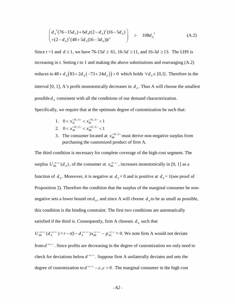
Since t >1 and 1≤d , we have 76-15d ≥ 61, 16-5d ≥11, and 16-3d ≥13. The LHS is

increasing in t. Setting t to 1 and making the above substitutions and rearranging (A.2)

reduces to ( )( )48 83 2 73 24 0A A Ad d d+ + − + > which holds [0,1]Ad∀ ∈ . Therefore in the

interval [0, 1], A’s profit monotonically decreases in Ad . Thus A will choose the smallest

possible Ad consistent with all the conditions of our demand characterization.

Specifically, we require that at the optimum degree of customization be such that:

1. , ,0 1SC S SC SAl Blx x< > < >< < <

2. , ,0 1SC S SC SAh Bhx x< > < >< < <

3. The consumer located at ,SC SBhx< > must derive non-negative surplus from

purchasing the customized product of firm A. The third condition is necessary for complete coverage of the high-cost segment. The

surplus )(,

ABh dU SSC >< , of the consumer at >< SSC

Bhx , , increases monotonically in [0, 1] as a

function of Ad . Moreover, it is negative at Ad = 0 and is positive at Ad = 1(see proof of

Proposition 2). Therefore the condition that the surplus of the marginal consumer be non-

negative sets a lower bound on Ad , and since A will choose Ad to be as small as possible,

this condition is the binding constraint. The first two conditions are automatically

satisfied if the third is. Consequently, firm A chooses Ad such that

)( ,, ><>< SSCSSC

ABh dU = ><><>< −−− SSCSSCSSC

ACBhA pxdtr ,,, )1( = 0. We note firm A would not deviate

from ,SC Sd < > . Since profits are decreasing in the degree of customization we only need to

check for deviations below ,SC Sd < > . Suppose firm A unilaterally deviates and sets the

degree of customization to , , 0SC Sd ε ε< > − > . The marginal consumer in the high cost

- A2 -

segment located at ( ), ,SC S SC SBh Ax d< > < > now derives negative surplus from purchasing the

customized product from firm A. This will result in incomplete coverage of the high cost

segment. To ensure sub-game perfection, we solve for the prices of the standard products

and the customized products under incomplete coverage for any given Ad . We substitute

these prices in firm A’s first stage profits and substitute ,SC SAd d ε< >= − . Following the

arguments in Lemma IV (in the Technical Supplement) we know that profits with

incomplete coverage are increasing in the degree of customization. In turn this implies

that firm A’s profits from deviating are decreasing in ε. It is therefore in firm A’s best

interest to set ε=0 or not to deviate.

QED

Proof of Lemma 3: Similar to the proof of lemma 2, for any given Ad , Bd we optimize

(7) with respect to ASp , ACp and (8) with respect to BSp and BCp . Solving the necessary

first-order conditions simultaneously we obtain the prices as a function of Ad and Bd . We

then substitute these prices in (7) and (8) to obtain the second stage profits of firms A and

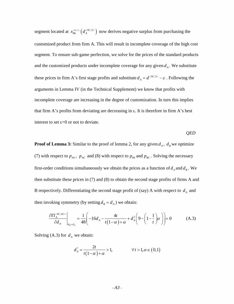
B respectively. Differentiating the second stage profit of (say) A with respect to Ad and

then invoking symmetry (by setting B Ad d= ) we obtain:

( ),

21 4 116 9 1 048 1

B A

SC SCA

A AA d d

td dd t t

αα α

< >

=

∂Π = − − + − − = ∂ − + (A.3)

Solving (A.3) for Ad we obtain:

( ) ( )* 2 1, 1, 0,11A

td tt

αα α

= > ∀ > ∈− +

- A3 -

( )( ) ( )* 2 0, 1, 0,19 1A

td tt

αα α

−= < ∀ > ∈

− +

Both these interior solutions are inadmissible since [ ]0,1Ad ∈ .

To characterize the equilibrium degree of customization we note that the derivative of

firm i’s second-stage profit with respect to id , evaluated at 1id = is negative.

{ }( )( )

( ) ( )( )( )

( )( ) ( )

( )( )

2 2

,

2

4 3 2

2 4 2

48 15 8 4

16 1 3 21144 2 1

15 38 2 16 214 108 108 352

A A A B B

SC SCA A BA

A A B

A A B A B B

b A B BA B

d d d d d

t d d dd d d t

d d d d d dtd d d dt d d

α α

α

< >

− + + + − − −∂Π = − ∂ − − − + − − − −− − + + − −− − (A.4)

Equation (A.4) evaluated at 1Ad = :

( )( ) ( ) ( )( )( ),

1

1 33 4 2 1 47 4 6 0144

A

SC SCA

B B B BA d

d d t t d dd t

α< >

=

∂Π −= − + + − + + <

∂ (A.5)

Thus A will choose the smallest possible Ad consistent with all the conditions of our

demand characterization. These consistency conditions are:

1. , , ,0 1SC SC SC SC SC SCAl ABl Blx x x< > < > < >< < < <

2. , , ,0 1SC SC SC SC SC SCAh ABh Bhx x x< > < > < >< < < <

3. The consumer located at ,SC SCABhx< > must derive non-negative surplus from

purchasing the customized product of either firm. The third condition is required for complete coverage of the high-cost segment. The

surplus )(,

AABh dU SCSC >< , of the consumer at >< SCSC

ABhx , , increases monotonically in [0, 1] as a

function of Ad , and as in Lemma 2, it is negative at Ad = 0 and is positive at Ad = 1(see

proof of Proposition 2). By a logic exactly similar to Lemma 2, firm A chooses Ad such

- A4 -

that )( ,, ><>< SCSCSCSC dU ABh = ><><>< −−− SCSCSCSCSCSC

ACABh pxdtr ,,, )1( = 0. We note that neither firm would

deviate from ,SC SCd < > . Since profits are decreasing in the degree of customization we only

need to check for deviations below ,SC SCd < > . Suppose firm A unilaterally deviates and sets

the degree of customization to , , 0SC SCd ε ε< > − > . Given firm B’s degree of customization,

,SC SCd < > the marginal consumer in the high cost segment located at

( ), , ,,SC SC SC SC SC SCABh A Bx d d< > < > < > now derives negative surplus from purchasing the customized

product from firm A. This will result in incomplete coverage of the high cost segment.

Therefore, to ensure sub-game perfection, we solve for the prices of the standard products

and the customized products under incomplete coverage for any given Ad and Bd . We

substitute these prices in the deviating firm’s first stage profits and substitute

,SC SCAd d ε< >= − and ,SC SC

Bd d < >= . Following the arguments in Lemma IV and Lemma V

(in the Technical Supplement) we know that profits with incomplete coverage are

increasing in the degree of customization. In turn this implies that the deviating firm’s

profits are decreasing in ε. This is illustrated in the following plot.

0.1 0.2 0.3 0.4 0.5

0.38

0.42

0.44

asc,scwith Incomplete Coverage

- A5 -

The above figure illustrates that it is in the deviating firm’s best interest to set ε to zero.

In other words deviating from ,SC SCd < > is not optimal.

QED

Proof of Proposition 1: The equilibrium prices and profits when both segments are

covered with only standard products are obtained by standard methods.. The optimal

prices are: )1/(2 ttpp BA +== , and optimal profits are )1/( ttBA +=Π=Π .

Suppose A deviates from offering only standard products to offering both standard and

customized products. A’s profit from such a switch in strategy is ><Π SSCA

, -k, where

><Π SSCA

, can be obtained from lemma 2 and equals

)1()2(288)259)(1(2)3(32)1(5384576

,

3,2,24,2,2

ttdttdttdtdtdt

SSC

SSCSSCSSCSSC

+−++++−+−−

><

><><><><

Subtracting the above expression from )1/( tt + gives

)1()2(288)}259)(1(2)3(32)1(596{

,

3,,23,2,

ttdttdttdtdtd

SSC

SSCSSCSSCSSC

+−++−++++

><

><><><><

(A.6)

Clearly, the denominator is positive. Consider the third and fourth terms inside the braces

in the numerator. Since 3+t > 1+t we substitute 3+t by 1+t in the third term and collect

terms to obtain the inequality

)259)(1(2)3(32)1(596 3,,23,2 ttdttdtdt SSCSSCSSC ++−++++ ><><>< >

><><>< ++−+++ SSCSSCSSC dttdttdt ,2,23,2 )1))(259(232()1(596 (A.7)

Since >< SSCd , < 1, )1(18)259(232 2, ttdt SSC +−>+− >< , and so the RHS of inequality (A.7)

is larger than ><+− SSCdtt ,22 )1(1896 . This quantity is, in turn, larger than

- A6 -

183678 2 −− tt since >< SSCd , < 1. Finally, 183678 2 −− tt > 0 if t > .764. Since t > 1, the

numerator of (A.6) and thus the entire quantity is positive. QED

Proof of Theorem 1:

To establish the proposition we will show that for intermediate values of t one firm, say

firm A will deviate from < S, S > to < SC, S >, and for high values of t firm B will deviate

from < SC, SC > to < SC, S >. In other words, for intermediate values of t the equilibrium

is < SC, SC > and for high values of t the equilibrium is < SC, S >.

Define:

:)(rt ∗∗ ><Π SSCA

, -k = ><Π SSA

, (A.8)

:)(rt ∗∗∗ ><Π SSCB

, = ><Π SCSCB

, -k (A.9)

We need to show that when ( ) ( )** ***,t t r t r ∈ the equilibrium first stage outcome is

<SC, SC >. This will be accomplished by showing that there exists )(** rt such that if t >

)(** rt then firm A will deviate from <S, S > to <SC, S >, and that there exists )(*** rt such

that, if t > )(*** rt then firm B will deviate from <SC, SC > to <SC, S >. Consider first the

proposed deviation by firm B.

B’s Deviation from <SC, SC > to <SC, S >:

Such a deviation will occur if ),(, ,,( trSSC

BSSCdt ><><Π ) > ,,

( , )( , )SC SC

A

SC SCr tB t d < >< >Π -k for all t >

)(*** rt . The strategy of proof is as follows:

We will show numerically that for small t,

(i) ,,( , )( , )SC SC

A

SC SCr tB t d < >< >Π -k > ),(

, ,,( trSSC

BSSCdt ><><Π ).

- A7 -

(ii) We will show that, there exists 0t large enough, such that for t > 0t ,

)],(),([ ),(,

),(, ,,

trSSC

BtrSCSC

BSSCSCSC dtdt

dtd ><>< ><>< Π−Π <0.

(iii) The above two statements imply that the difference

, ,, ,( , ) ( , )[ ( , ) ( , )]SC SC SC S

A

SC SC SC Sr t r tB Bt d t d< > < >< > < >Π −Π will start positive for small t and,

as t increases it will become negative for large enough t. Thus there will exist

)(*** rt , defined by ),(),( ),(,

),(, ***,***,

trSSC

BtrSCSC

BSSC

A

SCSC dtkdt ><>< ∗∗∗><∗∗∗>< Π=−Π

such that, for all t > )(*** rt , ),(, ,,( trSSC

BSSC

Adt ><><Π )-k > ),( ),(, ,

trSCSC

BSCSCdt ><><Π .

Proof of Statement (i):

Recall that 2r ≥ and following lemma 1, ( )* 2,t t r≥ = for 2r = . Recall that t is the

intensity of preference or the transportation cost parameter of the high cost segment.

Because the transportation cost parameter of the low cost segment is normalized to one, t

represents the intensity of preference of the high cost segment relative to the low cost

segment. In establishing this statement we substitute ( )* 0.001t t r= + in the expression

( ) ( ), ,, ,( , ) ( , ), ,SC SC SC S

A

SC SC SC Sr t r tB Bt d t d< > < >< > < >Π −Π so that the difference in firm B’s profits in

sub-games <SC,SC> and <SC,S> is only a function r. We vary r in the interval 2 to 10 to

obtain a plot of ( ) ( ), ,, ,( , ) ( , ), ,SC SC SC S

A

SC SC SC Sr t r tB Bt d t d< > < >< > < >Π −Π as a function of r (Figure

A1). Figure A1 demonstrates that for all r in the interval 2 to 10 the difference in profits

( ) ( ), ,, ,( , ) ( , ), ,SC SC SC S

A

SC SC SC Sr t r tB Bt d t d< > < >< > < >Π −Π is positive. Also note that for r = 10,

( )* 10 16.4t t≥ = , which is actually a very high value of t as it represents markets where

the transportation cost parameter of consumers in the high cost segment is at least 16.4

times that of consumers in the low cost segment.

- A8 -

4 6 8 10r

0.01

0.02

0.03

0.04

0.05bsc,scbsc,s

Figure A1. Firm B’s Incentive to Deviate and Reservation Price

We conclude therefore that for small t ( ) ( ), ,, ,( , ) ( , ), ,SC SC SC S

A

SC SC SC Sr t r tB Bt d t d< > < >< > < >Π > Π .

Proof of statement (ii):

)],(),([ ),(,

),(, ,,

trSSC

BtrSCSC

BSSC

A

SCSC dtdtdtd ><>< ><>< Π−Π = (

tt

SSCB

SCSCB

∂Π∂

−∂

Π∂ ><>< ,,

) +

(dt

ddddt

ddd

SSC

A

SCSC SSCB

SCSCB

><><

∂Π∂

−∂

Π∂ ><>< ,, ,,

) (A.10)

Next, we note that the profit of B in the < SC, S > case decreases in d. Observe that

)1()2(72))21(8)1(320)()2)(6(( 22,

ttdtdtdttddd

d

SSCB

+−+−++−−+

−=∂

Π∂ ><

< 0,∀ t and ∀ d <1.

Similarly, )1(3232)1(3 222,

ttttd

d

SCSCB

+−+

=∂

Π∂ ><

< 0, ∀ t and ∀ d <1, and finally

)1(288)17)(1(16)1(39))2/(64(1648 222,,

tttttddt

dd

SSCB

SCSCB

+−+−+−−+−

=∂

Π∂−

∂Π∂ ><><

> 0

Therefore

- A9 -

dd

SSCB

SCSCB

∂Π∂

>∂

Π∂ ><>< ,,

(A.11)

Thus the profit of firm B decreases wrt the degree of customization d more steeply in the

duopoly case than in the monopoly case.

Also the profits of firm B increase wrt t in both the monopoly and duopoly case.

2

3

2

,

32)1(1

td

td

t

SCSCB −

+−

=∂

Π∂ ><

> 0, and )2(72

)1()23(16

2

4

2

2

,

dtd

td

t

SSCB

−

−+−

=∂

Π∂ ><

>0, ∀ t and ∀ d <1.

Comparing the two slopes we find that the profit of firm B increases wrt t more steeply in

the monopoly customization case than in the duopoly customization case. That is

tt

SCSCB

SSCB

∂Π∂

>∂

Π∂ ><>< ,,

> 0 (A.12)

Lastly, we need to sign dtdd trSSC

A /),(, >< and dtdd tr

SCSC /),(, >< . We first consider

dtdd trSCSC /),(

, >< . The optimal ),(,

trSCSCd >< is obtained from the condition that the marginal

high-cost consumer ),(,

dtABhSCSCx >< that is indifferent between firm A’s customized product

and firm B’s customized product will receive zero surplus. Define ),( , >< SCSCdtU AC as the

utility of this marginal consumer indifferent between the two firms’ customized products.

Making substitutions for optimal quantities we get the surplus as a function of t and d

such that ),(,

trSCSCd >< solves ),( , >< SCSCdtU AC =0. Totally differentiating this w.r.t t gives

dtdd SCSC >< ,

= d

Ut

U ACAC

∂∂

∂∂

− /

Evaluating the partial derivatives on the RHS gives

dtdd SCSC >< ,

= ))1(2)5()(1(

)52)(1( 2

tdtttttd

+−++++− > 0.

- A10 -

Using an analogous technique it can be shown that dt

dd SSC

A

>< ,

> 0 (see treatment of A’s

deviation below). It remains for us to determine the relative magnitudes of dt

dd SSC

A

>< ,

and

dtdd SCSC >< ,

.

Claim: For any arbitrary ε >0, there exists 0t such that for t > 0t , ε<∂

∂−

∂∂ ><><

td

td SSC

A

SCSC ,,

.

In other words, for large enough t the rate of change in ),(,

trSCSCd >< is arbitrarily close to

rate of change in ),(,

trSSC

Ad >< .

Proof of claim: Since ),(,

trSCSCd >< increases in t, consider 1t large enough such that

),( 1

,tr

SCSCd >< lies within a 1ε -neighborhood of 1 for arbitrary 1ε >0. Clearly any further

increase in t to δ+1t will still keep ))(,( 1

,δ+

><tr

SCSCd in that neighborhood since ≤>< SCSCd , 1.

Therefore, 1),( /, ε≤>< dtdd trSCSC , 1tt ≥∀ . Similarly there exists 2t and 2ε such that

2),( /, ε≤>< dtdd trSSC

A , 2tt ≥∀ . Let 0t = max{ 1t , 2t }. By Schwarz inequality, we have

εεε =+<∂

∂−

∂∂ ><><

21

,,

td

td SSC

A

SCSC

(say), 0tt ≥∀ .

Let the quantity on the LHS of (A.10) be evaluated for t > 0t . Rewriting (A.8) so as to

reflect the signs of the various quantities on the R.H.S yields

)],(),([ ),(,

),(, ,,

trSSC

BtrSCSC

BSSC

A

SSC dtdtdtd ><>< ><>< Π−Π = (

tt

SSCB

SCSCB

∂Π∂

−∂

Π∂ ><>< ,,

) -

( )()(,, ,,

dtdd

ddtdd

d

SSC

A

SCSC SSCB

SCSCB

><><

∂Π∂

−∂

Π∂ ><><

) (A.13)

- A11 -

In light of inequalities (A.11) and (A.12), and the fact that dtdd trSSC

A /),(, >< is arbitrarily

close to dtdd trSCSC /),(

, >< , the quantity on the RHS of (A.13) is negative. This establishes

statement (ii) above.

A’s Deviation from <S, S > to <SC, S >:

Now, consider the proposed deviation by firm A. Such a deviation will occur if

),(, ,,( trSSC

ASSC

Adt ><><Π )-k > )(, tSSA

><Π for all t > )(** rt . We need to show that such a )(** rt

will indeed exist. The strategy of proof is exactly the same as that for B’s deviation.

Consider

)](),([ ,),(

, , tdtdtd SS

AtrSSC

ACSC

A

><>< Π−Π >< = t

SSCA

∂Π∂ >< ,

+ dt

ddd

SSC

A

SSCA

><

∂Π∂ >< ,,

- t

SSA

∂Π∂ >< ,

(A.14)

We have already established that t

SSA

∂Π∂ >< ,

< 0. Further,

)2(288

)18()1(

)3(64),(

,

,,,

, 2

3

2

2

,

><

><><><

><

−

−−

+−

=∂

Π∂ ><

SSC

A

SSC

A

SSC

A

SSC

ASSC

A

dt

ddt

d

tdtSSC

A > 0, and

+−−−

+

−−−

+

−−−

=∂

Π∂

><

><><

><

><><><

><><

><

><><

)1()2()1)(3(64

)2())1576(108(

)316(48

2881),(

2

2

2,

,

,,

,

,,,

,,

,

,

tddd

tdddd

dd

ddt

SSC

A

SSC

A

SSC

A

SSC

A

SSC

A

SSC

A

SSC

A

SSC

A

SSC

A

SSC

A

SSC

A

SSCA < 0

The last inequality holds because the first two terms dominate the third and fourth terms.

Finally, we have to sign dtdd trSSC

A /),(, >< . Recall that the optimal ),(

,tr

SSC

Ad >< is obtained from

the condition that the marginal consumer ,SC SBhx< > that is indifferent between firm A’s

customized product and firm B’s standard product will receive zero surplus. Defining

- A12 -

),( , >< SSC

AdtU AC as the surplus of this marginal consumer and making substitutions for

optimal quantities we get the surplus as a function of t and d such that ),(,

trSSC

Ad >< solves

),( , >< SSC

AdtU AC =0. Totally differentiating this w.r.t. t gives

dtdd SSC

A

>< ,

= d

Ut

U ACAC

∂∂

∂∂

− /

Evaluating the partial derivatives on the RHS gives

dtdd SSC

A

>< ,

= )179()113(4)5(6)1(2

)33)(1)(2(223

)1()33(4

2

2

tdtdtttd

dtdt

dd

+++−+++−

+−+−++−

. The numerator is clearly

positive and the denominator is decreasing in d. If we evaluate the denominator at d =1

(the lowest possible value of the denominator), we get a positive quantity, and so the

denominator is always positive. Thus, dtdd trSSC

A /),(, >< > 0, and moreover by repeated

applications of L’Hospital’s rule it can be shown that ∞→tlimdt

dd SSC

A

>< ,

=0. In other words,

for t large enough dtdd trSSC

A /),(, >< is negligibly small, and thus, the RHS of (A.14) is

positive. Hence, there exists a critical )(** rt such that )(),( ,),(

, , tdt SSAtr

SSCA

SSC

A

><>< Π−Π >< >k

for t > )(** rt . This constitutes a necessary and sufficient condition for firms to offer

customized products and A will deviate from < S, S > to < SC, S > for this range of

parameters. Said differently, for large t the direct effect of t on ><Π SSCA

, dominates the

indirect effect through ),(,

trSSC

Ad >< . Since the direct effect of increasing t increases ><Π SSCA

, ,

firm A will find it optimal to deviate to < SC, S >.

- A13 -

Finally, we need to put some restrictions on k. Note that )(** rt is increasing in k, and

)(*** rt is decreasing in k. Therefore we need k to be small enough such that ***t > **t . Let

**k be such that ***t = **t when k = **k . We need k < **k .

Lastly, we can show that ***t > **t for at least some values of r. To do so, it is enough to

show the existence of 1t and 2t , with 2t > 1t such that when t = 1t then < SC, SC > strictly

dominates < SC, S > for firm B, and when t = 2t then < SC, S > strictly dominates < SC,

SC >. This we do by construction. Let r =2, its minimum value. The minimum value of t

required for incomplete coverage of the standard product market is )2(*t = 2. We need 1t

> )2(*t , so let 1t =2.5. With these values of r and t, and with k=0.01, the optimal profits

with standard products are ><>< Π=Π SSB

SSA

,, = 0.45. If firm A offers a customized product

then the optimal quantities are >< SSC

Ad , = 0.511, ><Π SSCA

, = 0.618 and ><Π SSCB

, =0.456. So firm

A will deviate from < S, S > to < SC, S >. If firm B responds with its own customized

product the optimal quantities are >< SCSCd , = 0.2666, ><Π SCSCA

, = ><Π SCSCB

, = 0.524. Thus we

have < SC, SC > in equilibrium. Let 2t =10. We then have ><>< Π=Π SSB

SSA

,, = 0.3, >< SSC

Ad , =

0.949, ><Π SSCA

, = 0.644 and ><Π SSCB

, =0.35, so that A will offer its customized product.

However, >< SCSCd , = 0.748, and ><Π SCSCA

, = ><Π SCSCB

, = 0.233, so that B will not offer its

customized product. Thus we have < SC, S > in equilibrium. So for r = 2, 2t ≥ ***t ≥ 1t >

**t , establishing that ***t > **t .

QED

- A14 -

Proof of Proposition 2:

The optimum ),(,

trSSCd >< and ),(

,tr

SCSCd >< in the monopoly and duopoly customization cases

are both obtained from the condition that the marginal consumer indifferent between the

two firms products receives zero surplus. In the first case the marginal consumer >< SSC

Bhx , is

the one that is indifferent between firm A’s customized and firm B’s standard product

and, in the second case, the marginal consumer >< SCSC

ABhx , is the one that is indifferent

between firm A’s customized product and firm B’s customized product.

In equilibrium, the consumer at >< SSC

Bhx , derives a surplus of

)( ,, ><>< SSCSSC dU Bh = ),(),(,,,,, )1( ><><><><><

−−− SSCSSCSSCSSCSSCdtACdtBh pxdtr where we write the surplus as

a function of >< SSCd , . Making the appropriate substitutions, the optimal degree of

customization >< SSCd , solves

)1)(2(6

)}5()1(2{6)}5()1({6)113()1() (,

,,,,,

23

tdtttrtttrdtdtddU

SSC

SSCSSCSSCSSCSSC

Bh +−+++−−+−+−+−+

=><

><><><><><

= 0, where >< SSCd , is restricted to lie between 0 and 1.

Similarly, in duopoly customization >< SCSCd , solves

)1(2

)1(2)5()5()1() (,,

,,

2

ttrttttdtddU

SCSCSCSCSCSCSCSC

ABh ++++−+−+−

=><><

><>< = 0, where >< SCSCd , is

restricted to lie between 0 and 1.

Now consider )(, dU SSC

Bh>< and )(, dU SCSC

ABh>< as functions of d. We first note that ) (0, >< SCSC

ABhU =

) (0, >< SSC

BhU = )1(2

)1(2)5(t

trtt+

+++− < 0, the last inequality following from the fact that t > r.

Secondly, we note that (1), >< SSC

BhU > 0, ) (1, >< SCSC

ABhU > 0, and ) (1, >< SCSC

ABhU - (1), >< SSC

BhU =

)1(3)37(

tt++ > 0.

- A15 -

In other words, both )(, dU SSC

Bh>< and )(, dU SCSC

ABh>< start from the same negative value at d = 0,

and finally at d = 1 we find that )(, dU SCSC

ABh>< ends up at a higher positive value than

)(, dU SSC

Bh>< .

Lastly, it can be shown that 0

,

0

,

)()(=

><

=

><

∂∂

>∂

∂

d

SSCBh

d

SCSCABh

dU

dU , and that both )(, dU SSC

Bh>< and

)(, dU SCSC

ABh>< are monotonically increasing in [0, 1].

Therefore the graph of )(, dU SCSC

ABh>< starts higher than the graph of )(, dU SSC

Bh>< at d = 0, and

remains higher throughout the interval [0, 1]. This implies that, both )(, dU SSC

Bh>< and

)(, dU SCSC

ABh>< start from the same negative quantity at d = 0 and, as d increases,

)(, dU SCSC

ABh>< hits zero before )(, dU SSC

Bh>< (i.e. at a smaller value of d).

Therefore, in equilibrium,

),(,

trSSCd >< > ),(

,tr

SCSCd >< .

QED

Proof of Proposition 3: We start by noting that, following a logic similar to theorem 1

we can show that for t>r, firm A will deviate from <S, S> to <SC, S>. Also, following

similar steps as in theorem 1, we can show that dt

dd SSC

A

>< ,

>0, and dt

dd SCSC

A

>< ,

>0. Moreover,

since )(, td SSC >< > )(, td SCSC >< for all values of t, the maximum admissible t, denoted

by maxt , is such that )( max, td SSC >< =1. For any value of t > maxt , the surplus of the marginal

consumer at >< SSC

Bhx , will be negative. Recall that this consumer receives a surplus of

))(,( ,, tdtU SSCSSC

Bh><>< = ),(),(

,,,,, )1( ><><><><><−−− SSCSSCSSCSSCSSC

dtACdtBh pxdtr when her preference

intensity is t and when firm A offers a customized product with degree of

- A16 -

customization )(, td SSC >< . Note the dependence of the consumer surplus on t, both

explicitly, and implicitly through the degree of customization. Now, ))(,( ,, tdtU SSCSSC

Bh><><

decreases in t and so the maximum allowable value of t is obtained by solving

)1,( max, tU SSC

Bh>< =0, which yields maxt = 2/)13( −r . As in theorem 1, we can show that for t

large enough, , ,, ,( , ) ( , )[ ( , ) ( , )]SC SC SC S

A

SC SC SC Sr t r tB B

d t d t ddt

< > < >< > < >Π −Π < 0. In other words, if

<SC, S> can be an equilibrium outcome, it can only be when t is large enough.

Contrarily, we will show that firm B will deviate from <SC, S > to <SC, SC> even

at the largest possible t, and so <SC, S > cannot be an equilibrium. Firm B’s profit in the

<SC, S> subgame at >< SSCd , =1 and t = 2/)13( −r is ><Π SSC

B, = )26/(2 −rr . In the <SC, SC>

subgame firm B will choose the degree of customization )(, td SCSC >< such

that ))(,( ,, tdtU SCSCSCSC

ABh><>< =0. At t = 2/)13( −r , >< SCSCd , = 4/))9481(3339( −+−− rrr .

With these values of >< SCSCd , and t, the profit of firm B without the fixed cost is

><Π SCSC

B, =

)13(512))9481(3397()13(32))9481(3339( 23

−−++−−+−+−−

rrrrrrrr

. It can be

checked that ><Π SCSC

B, > ><Π SSC

B, for r > 0.675. Since r ≥2, ><Π SCSC

B, exceeds ><Π SSC

B, by a large

margin and the inequality remains true for small k. Thus, ><Π SCSC

B, -k > ><Π SSC

B, as long as k is

small, and B will deviate to <SC, SC>.

For t> maxt there will be incomplete coverage of the market even with customized

products. With incomplete coverage, the optimal profits in the various subgames are

><Π SS

i, =

tr4

2

; ><Π SSC

A, =

)1(164)(4)(

,

,, 223

><

><><

−+−

SSC

SSCSSC

A

AA

dtrdrd , ><Π SSC

B, =

tr4

2

;

- A17 -

><Π SCSC

i, =

)1(164)(4)(

,

,, 223

><

><><

−+−

SCSC

SCSCSCSC

i

ii

dtrdrd . It is easily checked that for >< SSC

Ad , <1,

><Π SSC

A, > ><Π SS

A, , and for >< SCSC

Bd , <1, ><Π SCSC

i, > ><Π SSC

B, . Thus, for t>r the only Nash equilibrium

is <SC, SC>. QED

Proof of Proposition 4: We will adopt the viewpoint of firm A. Let us assume that firm

B commits to offering only its standard product. If A offers only its customized product

its profit is )1()2(72

))6)(2((,

,,2,,

2

ttdtddd

SC

SCSCSCSC

A

AAAA +−

+−−=Π

><

><><><>< . If it offers both its standard and

customized products, its profit ><Π SSCA

, can be obtained from lemma 2 and equals

)1()2(288)259)(1(2)3(32)1(5384576

,

,,,, 322422

ttdttdttdtdtdt

SSC

SSCSSCSSCSSC

+−++++−+−−

><

><><><><

. Since

>< SC

Ad , = >< SSC

Ad , = 1d (say), these profits can be directly compared and it can be shown that

><Π SSCA

, - ><Π SCA

, =t

td32

)1(31 + >0.

Suppose that B commits to offering only its customized product. If A does likewise its

profit is t

td CCCC A

A +−

Π><

><

1)1( ,

, , and if it offers both the standard and customized products, its

profit is )1(32

)1()1(32 22 3,,,

tttddt CSCCSC

CSC AAA +

++−=Π

><><>< . Since >< CC

Ad , = >< CSC

Ad , = 2d (say), the

profits can be directly compared, and ><Π CSCA

, - ><Π CCA

, =t

td32

)1(32 + >0.

Finally, if B commits to offering both its customized and standard products, then A’s

profit from offering only its customized product ist

td CSC

A

+− ><

1)1( ,

. Its profit from offering

- A18 -

both a standard and a customized product is obtained from lemma 3. Again, A will make

greater profit by offering both products. QED

- A19 -