Algorithmica (2017) 78:714–740DOI 10.1007/s00453-016-0201-4

On Easiest Functions for Mutation Operators inBio-Inspired Optimisation

Dogan Corus2 · Jun He1 · Thomas Jansen1 ·Pietro S. Oliveto2 · Dirk Sudholt2 ·Christine Zarges1

Received: 30 September 2015 / Accepted: 9 August 2016 / Published online: 18 August 2016© The Author(s) 2016. This article is published with open access at Springerlink.com

Abstract Understanding which function classes are easy and which are hard for agiven algorithm is a fundamental question for the analysis and design of bio-inspiredsearch heuristics.Anatural starting point is to consider the easiest andhardest functionsfor an algorithm. For the (1+1) EA using standard bit mutation (SBM) it is well knownthat OneMax is an easiest function with unique optimum while Trap is a hardest.In this paper we extend the analysis of easiest function classes to the contiguoussomatic hypermutation (CHM) operator used in artificial immune systems. We definea function MinBlocks and prove that it is an easiest function for the (1+1) EA usingCHM, presenting both a runtime and a fixed budget analysis. Since MinBlocks is,up to a factor of 2, a hardest function for standard bit mutations, we consider theeffects of combining both operators into a hybrid algorithm. We rigorously prove thatby combining the advantages of k operators, several hybrid algorithmic schemes haveoptimal asymptotic performance on the easiest functions for each individual operator.In particular, the hybrid algorithms using CHM and SBM have optimal asymptoticperformance on bothOneMax andMinBlocks.We then investigate easiest functionsfor hybrid schemes and show that an easiest function for a hybrid algorithm is not justa trivial weighted combination of the respective easiest functions for each operator.

Keywords Running time analysis · Theory · Hybridisation · Evolutionaryalgorithms · Artificial immune systems

B Christine Zargesc.zarges@aber.ac.uk

1 Department of Computer Science, Aberystwyth University, Aberystwyth SY23 3DB, UK

2 Department of Computer Science, University of Sheffield, Sheffield S1 4DP, UK

123

Algorithmica (2017) 78:714–740 715

1 Introduction

Over the past years many bio-inspired search heuristics such as evolutionary algo-rithms, swarm intelligence algorithms, or artificial immune systems, have beendeveloped and successfully applied to various optimisation problems. These heuristicshave different strengths and weaknesses in coping with different fitness landscapes.Determining which heuristic is the best choice for a given problem is a fundamentaland important question.

We use rigorous theoretical analyses to contribute to a better understanding of bio-inspired algorithms. A natural step is to investigate which functions are easy andwhichare hard for a given algorithm as this yields fundamental insights into their workingprinciples, particularly with respect to their strengths and weaknesses.

Knowing how well an algorithm performs on its easiest and hardest functions, withregards to the expected optimisation time, provides general insights, as the expectedoptimisation time of every function will be no less than that of an easiest function andnomore than that of a hardest function.With respect to applications, such researchmayalso provide guidelines for the design of benchmarks for experimental studies [10].

For a simple elitist (1+1) evolutionary algorithm (EA) using only standard bitmutations (SBM) Doerr, Johannsen, and Winzen showed that OneMax, a functionsimply counting the number of ones in a bit string, is the easiest problem among allfunctions with a single global optimum [8]. This statement generalises to the class ofall evolutionary algorithms that only use standard bit mutation for variation [33] aswell as higher mutation rates and stochastic dominance [37]. On the other hand, Heet al. [10] showed that the highly deceptive function Trap is the hardest function forthe (1+1) EA.

In this work we consider typical mutation operators in artificial immune systemswhere no such results are available.Mutation operators in artificial immune systems [6]usually come with much larger mutation rates than mutation operators in evolution-ary algorithms. One such example is the somatic contiguous hypermutation (CHM)operator from the B-cell algorithm (BCA) [23], where large contiguous blocks of abit string are flipped simultaneously. Previous theoretical work on comparing SBMand CHM has contributed to the understanding of their benefits and drawbacks in thecontext of its runtime on different problems [14,17,18], the expected solution qualityafter a pre-defined number of steps [21], and in dynamic environments [22]. It is easyto see that hardest functions for CHM with respect to expected optimisation times arethose where the algorithm gets trapped with positive probability such that the opti-misation time is not finite, e. g., if there exists a second best search point for whichall direct mutations to the optimum involve non-contiguous bits [17]. However, it isan open problem and the next step forward to determine what kind of functions areeasiest for this type of mutation operator.

The BCA uses standard bit mutations alongside CHM and thus can be consideredas a hybrid algorithm combining two mutation operators. More specifically, it usesa population of search points and creates λ clones for each of them. It then appliesstandard bit mutation to a randomly selected clone for each parent search point andsubsequently applies CHM to all clones. The interplay between these two operatorshas been investigated for the vertex cover problem [14].

123

716 Algorithmica (2017) 78:714–740

Hybridisations such as hyper-heuristics [30] and memetic algorithms [27] havebecome very popular over recent years. But despite their practical success their theoret-ical analysis is still in its infancy, noteworthy examples being thework in [1,24,32,34].However, nothing is known about easiest or hardest functions for such algorithms.

The goals of this paper are twofold. We first want to understand what functions areeasy for CHM and investigate the performance of CHM and SBM on these functions.Afterwards we consider hybridisations of SBM and CHM and easiest functions forsuch algorithms. We first use the method by He et al. [10], explained in Sect. 3, toderive an easiest function for CHM which we callMinBlocks. In Sect. 4 we presentan analysis of the optimisation time as well as a fixed budget analysis for CHM onMinBlocks. We then show that SBM alone is not able to optimise the constructedfunction and that a hybridisation of SBM and CHM can have significant advantages(Sect. 5.1). Finally, we investigate properties of easiest functions for such hybridalgorithms (Sect. 5.3).

This journal paper extends a preliminary conference paper [4] in several ways.Firstly, in Sect. 3 it is discussed how the framework for determining easiest and hardestfunctions is not restricted to (1+1)-style algorithms, but is general enough to applyfor a much larger class of algorithms including (1+λ) EAs [13] and the recentlypopular (1+(λ, λ)) GA using mutation and crossover [7]. Secondly, the analysis of theadvantages of hybridisation in Sect. 5.1 has been considerably extended. Rather thanjust giving an example of a hybrid algorithm using one out of two operators at eachstep with constant probability, the analysis has been generalised to allow differenthybridisation schemes and an arbitrary number k of operators. Finally, in Sect. 5.2 anexperimental analysis is presented to shed light on the performance of the algorithmsfor fitness functions that depend both on the number of ones (i.e., OneMax) and thenumber of blocks (MinBlocks) in the bit string.

2 Preliminaries

We are interested in all strictly elitist (1+1) algorithms with time independent variationoperators which we formally define in Algorithm 1 for maximisation problems. Werefer to any algorithm belonging to this scheme as a (1+1) A. This generalised algo-rithmic scheme keeps a single solution x as a population and creates a single offspringat every generation. The new offspring is accepted if it is strictly fitter than the parent.The algorithm outputs the best found solution once a termination condition is satisfied.Since in this paper we are interested in the expected number of steps required by thealgorithm to find an optimal solution, we will assume that the algorithm runs foreverand we will call runtime the number of fitness function evaluations performed beforethe first point in time when the optimum is found.

Different algorithms are obtained from the (1+1) A scheme by using differentvariation operators in line 1 of Algorithm 1. Apart from the explicit requirement oftime independence, the variation operators are implicitly restricted to the domain ofunary variation operators since the population size is one. In this paperwewill considertwo different mutation operators that accept a bit string x ∈ {0, 1}n as input. The first isthe most common unary variation operator, called standard bit mutation (SBM). This

123

Algorithmica (2017) 78:714–740 717

Algorithm 1 (1+1) A1: input: fitness function f ;2: generate an initial solution x uniformly at random;3: while termination condition is not satisfied do4: y ← is mutated from parent x ;5: if f (y) > f (x) then6: let x ← y;7: end if8: end while9: output: x .

variation operator flips each bit independently with probability 1/n. SBM is formallydefined in Algorithm 2.

Algorithm 2 Standard Bit Mutation (SBM)for i := 0 to n − 1 dowith probability 1/n set x [i] := 1 − x [i];

end for

Wewill refer to the (1+1) A that uses SBM as the (1+1) EA, themost widely studiedevolutionary algorithm.

The other variation operator of interest is the contiguous hypermutation operator(CHM), which mutates a bit string by picking a bit position and flipping a randomnumber of bits that follow it (in a wrapping around fashion) each with probability r .As done in previous work (see, e. g., [17]), we only consider the extreme case hereand set r = 1. CHM is formally defined in Algorithm 3.

Algorithm 3 Somatic Contiguous Hypermutation (CHM)select p ∈ {0, 1, ..., n − 1} uniformly at random;select l ∈ {0, 1, ..., n} uniformly at random;for i := 0 to l − 1 dowith probability r set x [(p + i) mod n] := 1 − x [(p + i) mod n];

end for

We will refer to the (1+1) A that uses a CHM operator as (1+1) CHM.Note that Algorithm 1 uses strict selection, i. e. only strict improvements are

accepted. For most of our theoretical results we also consider a variant of Algorithm 1with non-strict selection, where the acceptance condition “ f (y) > f (x)” is replacedby “ f (y) ≥ f (x)”.

3 Easiest and Hardest Functions

Our work is based on previous work by He et al. [10]. We consider the problem ofmaximising a class of fitness functions with the same optima. An instance of theproblem is to maximise a fitness function f :

123

718 Algorithmica (2017) 78:714–740

argmaxx∈S

f (x), (1)

where S is a finite set.Let T (A, f, x) denote the expected number of function evaluations for the (1+1) A

to find an optimal solution for the first timewhen starting at x (expected hitting time). Inthe following we only consider algorithms and functions that lead to a finite expectedhitting time.

Definition 1 [10, Definition 1] Given a (1+1) A for maximising a class of fitnessfunctions with the same optima (denoted by F), a function f in the class is said to bean easiest function for the (1+1) A if T (A, f, x) ≤ T (A, g, x) for every g ∈ F andevery x ∈ S. A function f in the class is said to be a hardest function for the (1+1) Aif T (A, f, x) ≥ T (A, g, x) for every g ∈ F and every x ∈ S.

The above definition of easiest and hardest functions is based on a point-by-pointcomparison of the runtime of the EA on two fitness functions. The criteria stated inthe following Lemmas 4 and 5 for determining whether a fitness function is an easiestor hardest function for a (1+1) A were originally given in [10]. The main proof ideain [10] is to apply additive drift theorems [11], taking the expected hitting time as driftfunction (distance to the target state). We state these drift theorems as Theorem 2,referring to the presentation of Lehre and Witt [25], who provided a self-containedproof.

Theorem 2 (Additive Drift [11,25]) Let (Xt )t≥0 be a stochastic process over somebounded state space S ⊆ R

+0 , and let T be the first hitting time of state 0. Assume that

E (T | X0) < ∞. Then:

(i) If E (Xt − Xt+1 | X0, . . . , Xt ; Xt > 0) ≥ δu then E (T | X0) ≤ X0/δu.(ii) If E (Xt − Xt+1 | X0, . . . , Xt ) ≤ δ� then E (T | X0) ≥ X0/δ�.

Before presenting those criteria, we state and prove the following helper lemma. Itis stated as Lemma 3 in [10] without proof.

Lemma 3 If the expected time T (A, f, x) is used as the drift function, then theexpected drift1 is Δ f (x) = 1 for all non-optimal search points x.

Proof Let P(x, y) denote the probability that the search point y is adopted as thecurrent search point at the end of an iteration of the (1+1) A with current searchpoint x . Since

∑

yP(x, y) = 1,

T (A, f, x) =∑

y

P(x, y)T (A, f, x).

1 In drift analysis, a drift function is a non-negative function d(x) such that d(x) = 0 for an optimal pointand d(x) ≥ 0 for a non-optimal point. The expected drift at point x is E (d(x) − d(y)), where y is the nextiteration’s search point. The expected drift is denoted by Δ f (x) when maximising f (x), or Δ(x) in short.

123

Algorithmica (2017) 78:714–740 719

For all non-optimal search points x , the (1+1) A will spend one iteration and thencontinue from the search point reached during this transition, hence

T (A, f, x) = 1 +∑

y

P(x, y)T (A, f, y).

Together, we have

∑

y

P(x, y)T (A, f, x) −∑

y

P(x, y)T (A, f, y) = 1

⇔∑

y

P(x, y)(T (A, f, x) − T (A, f, y)

) = 1

⇔∑

y

P(x, y)(d(x) − d(y)

) = 1.

That is Δ f (x) = 1 for all non-optimal search points x . First, we have the following criterion of determining whether a fitness function is an

easiest function for a (1+1) A. The two lemmasbelowextendTheorem1andTheorem2in [10], respectively, as they are applicable to both strict elitist selection (that is, theparent x is replaced by the child y if f (y) > f (x)) and non-strict elitist selection (thatis, the parent x is replaced by the child y if f (y) ≥ f (x)). The framework in [10] wasrestricted to strict selection.

Lemma 4 Given a (1+1) Awith elitist selection (either strict or non-strict) and a classof fitness functions with the same optima, if the following monotonically decreasingcondition holds,

– for any two points x and y, if T (A, f, x) < T (A, f, y), then f (x) > f (y),

then f is an easiest function in this class.

Proof Let g(x) be any fitness function with the same optima as f (x). Choose theruntime T (A, f, x) as the drift function: d(x) = T (A, f, x).

When maximising f (x), according to Lemma 3, for any non-optimal point x thedrift Δ f (x) = 1. In the following we prove that the drift Δg(x) ≤ Δ f (x) = 1.

Let Pf (x, y) and Pg(x, y) denote the probability of mutating x into y (which isindependent of the function f or g) and then y being accepted (which is dependent onf or g) when optimising f and g, respectively. We separately consider the negativedrift Δ−

f (x) = ∑y:d(x)<d(y) Pf (x, y)(d(x) − d(y)) and the positive drift Δ+

f (x) =∑

y:d(x)>d(y) Pf (x, y)(d(x) − d(y)) and note that Δ f (x) = Δ+f (x) + Δ−

f (x) astransitions with d(x) = d(y) do not contribute to Δ f . The same notation is used forΔg .

Negative drift: let x and y be two points such that d(x) < d(y). According to themonotonically decreasing condition, f (x) > f (y). For f (x), since f (x) > f (y),

123

720 Algorithmica (2017) 78:714–740

y is never accepted and then Δ−f (x) = 0. But for g(x), the negative drift is not

positive. Thus we have

Δ−g (x) ≤ 0 = Δ−

f (x). (2)

Positive drift: let x and y be twopoints such thatd(x) > d(y). If y is an optimum, thennaturally f (x) < f (y). If y is not an optimum, then according to themonotonicallydecreasing condition, f (x) < f (y).

Let P [m](x, y) denote the probability of mutating x into y (which is independentof f or g).

For f (x), since f (x) < f (y), y is always accepted and then Pf (x, y) =P [m](x, y). But for g(x), since g(x) might be larger, smaller than or equal tog(y), Pg(x, y) ≤ P [m](x, y). Hence

Δ+g (x) =

∑

y:d(x)>d(y)

Pg(x, y)(d(x) − d(y))

≤∑

y:d(x)>d(y)

Pf (x, y)(d(x) − d(y)) = Δ+f (x).

Considering both negative drift and positive drift, we get Δg(x) ≤ Δ f (x) = 1.Since Δg(x) ≤ 1 for all x , according to Theorem 2, the expected runtime isT (A, g, x) ≥ d(x) = T (A, f, x) and the theorem statement is derived.

In a similar way, we have the following criterion of determining whether a fitnessfunction is a hardest function for a (1+1) A, assuming that all expected optimisa-tion times are finite2. The monotonically decreasing condition in the above lemma isreplaced by the monotonically increasing condition.

Lemma 5 Given a (1+1) Awith elitist selection (either strict or non-strict) and a classof fitness functions with the same optima, if the following monotonically increasingcondition holds,

– for any two non-optimal points x and y, if T (A, f, x) < T (A, f, y), then f (x) <

f (y),

then f is a hardest function in this class.

Proof Let g(x) be any fitness function with the same optima as f (x). Choose theruntime T (A, f, x) as the drift function: d(x) = T (A, f, x).

For f (x), according to Lemma 3, for any non-optimal point x the drift Δ f (x) = 1.For g(x), we prove that the drift Δg(x) ≥ Δ f (x) = 1, using the notation for positiveand negative drift from the proof of Lemma 4.

2 Hardest functions are formally only defined for functions and algorithmswith finite expected optimisationtimes. However, we regard functions leading to infinite expected times as being harder than those with finiteexpected times.

123

Algorithmica (2017) 78:714–740 721

Positive drift: let x and y be two points such that d(x) > d(y). Let P [m](x, y) denotethe probability of mutating x into y (which is independent of f or g). For f (x), ify is an optimum point, then the probability that x is mutated into y and is accepted,Pf (x, y), is equal to P [m](x, y). Similarly for g(x), Pg(x, y) = P [m](x, y) if y isan optimum point. If y is not an optimum point, according to the monotonicallyincreasing condition, f (x) > f (y). For f (x), since f (x) > f (y), the probabilityPf (x, y) = 0. But for g(x), since g(x) might be larger, smaller than or equal tog(y), Pg(x, y) ≥ 0. Thus we have Pg(x, y) ≥ Pf (x, y) for all (x, y) such thatd(x) > d(y). Therefore, the positive drifts for g and f satisfy

Δ+g (x) =

∑

y:d(x)>d(y)

Pg(x, y)(d(x) − d(y))

≥∑

y:d(x)>d(y)

Pf (x, y)(d(x) − d(y)) = Δ+f (x).

Negative drift: let x and y be two points such that d(x) < d(y). Then according tothe monotonically increasing condition, f (x) < f (y).

For f (x), since f (x) < f (y), y is always accepted and then Pf (x, y) =P [m](x, y). But for g(x), since g(x) might be larger, smaller than or equal tog(y), Pg(x, y) ≤ P [m](x, y). Hence

Δ−g (x) =

∑

y:d(x)<d(y)

Pg(x, y)(d(x) − d(y))

≥∑

y:d(x)<d(y)

Pf (x, y)(d(x) − d(y)) = Δ−f (x).

Considering both negative drift and positive drift, we get Δg(x) ≥ Δ f (x) = 1.Since Δg(x) ≥ 1 for all x , according to Theorem 2, the expected runtime isT (A, g, x) ≤ d(x) = T (A, f, x) and the theorem statement is derived.

The framework due to He et al. [10] is restricted to search heuristics that base theirsearch on a single point in the search space and it is not obvious how to expand thisto population-based algorithms. However, it is worth mentioning that the frameworkis not restricted to (1+1)-style algorithms. It can also be applied to algorithms thatemploy elitist selection but have a more complicated way of deciding on the nextsearch point to use as next parameter. Such algorithms can be described as (1+1)-stylealgorithms with a muchmore complex mutation operator or, perhaps more adequately,by exactly the same kind of Markov chain as that of a (1+1)-style algorithm, i. e., bya Markov chain of the same size 2n × 2n . Algorithms where this is true include the(1+λ) EA (see, e.g., [13]) that creates λ offspring bymeans of mutation, independentlyand identically distributed, and a best one replaces the current population if its fitnessis not worse. In this sense the framework can deal with population-based heuristics(given that the population is restricted to a larger offspring population, not a largerparent population). It can also be applied beyondmutation-based algorithms to geneticalgorithms with crossover if the restriction of a population of size only 1 is met. An

123

722 Algorithmica (2017) 78:714–740

example for such an algorithm is the so-called (1+(λ, λ)) GA [7], the first realisticevolutionary algorithm to provably beat theΩ (n log n) lower bound onOneMax. Wesee that the framework ismuchmore general and useful than itmay appear at first sight.

We have already mentioned that we consider functions where an algorithm doesnot have finite expected optimisation time to be harder than those with finite expectedoptimisation times. It is well known that CHM (Algorithm 3) can be trapped in localoptima when the parameter r is set to r = 1 [2] (see [17, p. 521] for a concreteexample demonstrating this effect). Setting r = 1, however, reveals properties of thehypermutation operator in the clearest way and this is the reason we stick to thischoice (compare [17]). This implies that analysing hardest functions for (1+1) CHMdoes not make much sense because it is easy to find functions where there is a positiveprobability that the algorithm gets stuck in a local optimum so that, consequently,the expected optimisation time is not finite. One could consider different measuresof hardness for this situation, e. g., considering the conditional expected optimisationtime given that a global optimum is found or, alternatively, considering the probabilitynot to find a global optimum. This, however, is beyond the scope of this article.

4 Contiguous Hypermutations on an Easiest Function with a UniqueGlobal Optimum

We are now ready to derive an easiest function with a unique global optimum forcontiguous hypermutations and analyse the performance of the (1+1) CHM on thisfunction.

4.1 Notation and Definition

We use x = x[0]x[1] · · · x[n − 1] ∈ {0, 1}n as notation for bit strings of length n. Fora, b ∈ {0, 1, . . . , n − 1} we denote by x[a . . . b] the concatenation of x[a], x[(a +1) mod n], x[(a + 2) mod n], …, x[(a + i) mod n] where i is the smallest numberfrom {0, 1, . . . , n − 1} with (a + i) mod n = b. We denote by |x[a . . . b]| the numberof bits in x[a . . . b], i. e., its length. We say that x ∈ {0, 1}n contains a 1-block froma to b if x[a . . . b] = 1|x[a...b]| and x[(a − 1) mod n] = x[(b + 1) mod n] = 0 hold.Analogouslywemay speakof a 0-block froma tob.Note that bit strings need to containat least one 0-bit and at least one 1-bit to contain a 0-block or a 1-block. It is easy to seethat each x ∈ {0, 1}n \ {0n, 1n} contains an equal number of 0-blocks and 1-blocks.

Definition 6 Wedefine an easiest functionwith unique global optimum for contiguoushypermutations by defining a partition L0 ∪̇ L1 ∪̇ L2 ∪̇ · · · ∪̇ Ll = {0, 1}n andassigning fitness values accordingly. We call the function MinBlocks and defineMinBlocks(x) = l− i for x ∈ Li . We define l = �n/2 +1 and level sets L0 = {1n},L1 = {0n} and Li = {x ∈ {0, 1}n | x contains i − 1 different 1-blocks} for eachi ∈ {2, 3, . . . , l}.

The function has a unique global optimum 1n with function value l = �n/2 + 1.The second best bit string is 0n with function value l − 1. All other bit strings containan equal number of 0-blocks and 1-blocks. A bit string with j 1-blocks is in level setL j+1 and thus, its function value equals l − ( j + 1) = l − j − 1.

123

Algorithmica (2017) 78:714–740 723

We defer the proof that MinBlocks is indeed an easiest function for (1+1) CHMto the next section (Theorem 8) in order to make use of arguments from the analysisof the expected optimisation time performed there.

4.2 Expected Optimisation Time

We analyse the expected optimisation time of the (1+1) CHM on MinBlocks, i. e.,the expected number of function evaluations executed until the global optimum isreached [12]. To facilitate our analysis, we start with an analysis of the expectedoptimisation time starting from a bit string from a particular level set which will inturn allow us to prove thatMinBlocks is an easiest function for (1+1) CHM.We willthen continue with the overall upper and lower bounds for the optimisation time.

Lemma 7 We consider (1+1) CHMwith strict or non-strict selection onMinBlocksas defined in Definition 6. For i ∈ {0, 1, . . . , l} (where l + 1 is the number of sets inthe partition from Definition 6) let Ti denote the random number of steps needed toreach the unique global optimum 1n when started in a bit string from Li . The expectednumbers of steps are E (T0) = 0, E (T1) = n + 1, E (T2) = (n + 1)2/2 and

E (Ti ) = n(n + 1)

(2i − 2)(2i − 3)+ E (Ti−1)

for all i ∈ {3, 4, . . . , l}.Proof The statement about E (T0) is trivial. For E (T1) it suffices to observe that anyhypermutation which chooses as mutation length n leads from 0n to the unique globaloptimum 1n . Such a mutation has probability 1/(n+1)which implies E (T1) = n+1.For E (T2) we observe that for each x ∈ L2 there are two mutations which lead toL0∪L1, one leading to L0 and the other leading to L1. Since L0 and L1 are reachedwithequal probability 1/2we haveE (T2) = n(n+1)/2+E (T1)/2 = (n+1)2/2. For E (Ti )with i > 2 we observe that only mutations that reduce the number of 1-blocks can leadto some L j with j < i . It is easy to see that, the number of 1-blocks can only be reducedby 1 in one contiguous hypermutation. In order to achieve that a mutation must startat the first bit of a block (either a 0-block or a 1-block) and end at the last bit of a block(either a 0-block or a 1-block) but this block cannot be the one just before the blockcontaining the first flipped bit (otherwise the length of the mutation is n, the bit stringis inverted and the number of 1-blocks remains unchanged). Thus, if there are j blocksin the bit string, the number of such mutations equals j ( j −1). For x ∈ Li the numberof 1-blocks equals i −1 and therefore the number of blocks equals 2i −2 so that thereare (2i − 2)(2i − 3) such mutations. Thus, the expected time to leave Li equals n(n+1)/((2i − 2)(2i − 3)) and E (Ti ) = n(n+ 1)/((2i − 2)(2i − 3))+E (Ti−1) follows.

The expected runtimes provided inLemma7allowus to verifywhetherMinBlockssatisfies the criteria set by Lemma 4. The following theorem establishesMinBlocksas an easiest function for (1+1) CHM.

Theorem 8 MinBlocks is an easiest function for the (1+1) CHM with strict or non-strict selection among all functions with a unique optimum.

123

724 Algorithmica (2017) 78:714–740

Proof The theorem follows from Lemma 7, the definition of MinBlocks, andLemma 4. According to Definition 6, for all i ∈ {1, 2, . . . , �n/2 } the fitness valueof solutions in subset Li is strictly less than the fitness value of solutions in Li−1.Therefore, a solution x has a better MinBlocks value than a solution y, if andonly if x and y belong to two distinct subsets Li and L j respectively such thati < j . Note that in Lemma 7 the expected runtime of the (1+1) CHM initialisedwith a solution from Li , E (Ti ), satisfies E (Ti ) > E (Ti−1) for all i and thus i < jimplies E (Ti ) < E

(Tj

). Therefore, MinBlocks(x) > MinBlocks(y) if and only

if the expected runtimes of (1+1) CHM starting from solutions x and y satisfyT (A, f, x) = E (Ti ) < E

(Tj

) = T (A, f, y). According to Lemma 4, the abovetwo way implication makes MinBlocks an easiest function for the (1+1) CHM.

We continue our analysis of the expected optimisation time. Note that the followingbound asymptotically matches the lower bound of Ω

(n2

)for contiguous hypermuta-

tions and functions with a unique global optimum proven by Jansen and Zarges [17].

Theorem 9 Let T denote the expected optimisation time of the (1+1) CHMwith strictor non-strict selection on MinBlocks. E (T ) = ln(2)n2 ± O (n) holds.

Proof Consider x ∈ {0, 1}n selected uniformly at random. For each i∈{0, 1, . . . , n−1}we have that a block ends at x[i] if x[i] �= x[(i+1) mod n] holds. Thus, x[i] is the endof a block with probability 1/2 and we see that the expected number of blocks equalsn/2. Let I denote the number of blocks. An application of Chernoff bounds yieldsthat for any constant ε with 0 < ε < 1 we have Pr (I ≥ (1 − ε)n/2) = 1 − e−Ω(n).

We know that E (T | I = 2(i − 1)) = E (Ti ) holds and have

E (Ti ) = n(n + 1)

(2i − 2)(2i − 3)+ E (Ti−1)

= n(n + 1)

(2i − 2)(2i − 3)+ n(n + 1)

(2(i − 1) − 2)(2(i − 1) − 3)+ E (Ti−2)

= · · · = E (T2) + n(n + 1)i−3∑

j=0

[1

(2(i − j) − 2)(2(i − j) − 3)

]

= E (T2) + n(n + 1)i−3∑

j=0

[1

2 j + 3+ 1

2 j + 4− 1

j + 2

]

= E (T2) + n(n + 1)

⎛

⎝

⎛

⎝2i−2∑

j=3

1

j

⎞

⎠ −⎛

⎝i−1∑

j=2

1

j

⎞

⎠

⎞

⎠

= E (T2) + n(n + 1)

(

H2i−2 − Hi−1 − 1

2

)

where Hj denotes the j th harmonic number. Using Hj = ln( j)+γ +1/(2 j)−o (1/j)(γ = 0.57721 . . . the Euler-Mascheroni constant) we obtain

123

Algorithmica (2017) 78:714–740 725

E (T | I = 2(i − 1)) = (n + 1)2

2+ n(n + 1)

(

ln(2) − 1

2

)

− O(n2/ i

)

= ln(2)n2 + O (n) − O(n2/ i

).

For the lower bound on E (T ) we use i = (n/8) + 1 (and have Pr (I ≥ n/4) =1 − e−Ω(n), of course) and obtain

E (T ) ≥ Pr (I ≥ n/4) · E (T | I ≥ n/4)

=(1 − e−Ω(n)

)·(ln(2)n2 + O (n) − O (n)

)= ln(2)n2 ± O (n)

as claimed.For the upper bound on E (T ) we have

E (T ) ≤ E(Tn/2

) = ln(2)n2 + O (n) − O (n) = ln(2)n2 ± O (n)

as claimed.

4.3 Fixed Budget Analysis

It has been pointed out that the notion of optimisation time does not always capture thenature of how randomised search heuristics are applied in practice. As a result, fixedbudget analysis has been introduced as an alternative theoretical perspective [19,20].Let xt denote the current population after t rounds of contiguous hypermutation andselection. In fixed budget analysis we want to analyse E ( f (xt )) for all t ≤ E (T )

where E (T ) is the expected optimisation time. We do this here for MinBlocks togive a more complete picture about the performance of the (1+1) CHM. Note that acomparison of the (1+1) EA and the (1+1) CHM under the fixed budget perspectivehas previously been performed for some example functions [21].

We begin with a statement about the expected function value of a uniform randomsolution, reflecting the way (1+1) A algorithms are initialised, and prove that it isroughly (n − 2)/4 ± 1/2.

Theorem 10 Let x0 ∈ {0, 1}n be selected uniformly at random and f := MinBlocksfrom Definition 6. For the initial function value E ( f (x0)) = �n/2 − (n/4) + 2−n

holds.

Proof We know from the analysis of the expected optimisation time in Sect. 4.2 thatthe expected number of blocks in x0 equals n/2. Let z(x0) denote the number of 0-blocks in x0 and remember that the number of 0-blocks is half the number of blocks.This implies E (z(x0)) = n/4.

Let l = �n/2 + 1 (the value defined in Definition 6). Remember that z(1n) =z(10) = 0 according to our definition of a 0-block (see the definition of the notationat the beginning of Sect. 4.1). For x0 /∈ {0n, 1n} we have f (x0) = l − 1 − z(x).Furthermore, we have f (1n) = l and f (0n) = l − 1 = l − 1− z(0n). Thus, f (x0) =l − 1 − z(x) holds always except for the case x0 = 1n .

123

726 Algorithmica (2017) 78:714–740

We have

E ( f (x0)) =∑

x∈{0,1}nf (x)

2n=

∑

x∈{0,1}n\{1n}

[l − 1 − z(x)

2n

]

+ l

2n

=∑

x∈{0,1}n\{1n}

[l − 1 − z(x)

2n

]

+ l

2n+ l − 1 − z(1n)

2n− l − 1 − z(1n)

2n

=∑

x∈{0,1}n

[l − 1 − z(x)

2n

]

+ l

2n− l − 1 − z(1n)

2n

=∑

x∈{0,1}n

[l − 1 − z(x)

2n

]

+ 1

2n= E (l − 1 − z(x0)) + 1

2n

= l − 1 − E (z(x0)) + 2−n = l − 1 − (n/4) + 2−n

and obtain the claimed bound by remembering that l = �n/2 + 1 holds. Wenowgive upper and lower bounds on the expected functionvalue after t iterations

of the (1+1) CHM.

Theorem 11 Let xt ∈ {0, 1}n denote the current search point after random initiali-sation and t rounds of contiguous hypermutation and strict or non-strict selection onf := MinBlocks. The following bounds hold for the expected function value after tsteps E ( f (xt )).

lower bound E ( f (x0)) +(⌊n

2

⌋+ 1 − E ( f (x0))

) (

1 −(

1 − 2

n(n + 1)

)t)

≤⌊n

2

⌋+ 1 −

(⌊n

2

⌋+ 1 − E ( f (x0))

)·(

1 − 3

n(n + 1)

)t

≤ E ( f (xt ))

upper bound E ( f (xt ))

≤n/2∑

z=1

[(n/2

z

)

2−n/2 ·((n

2− z

)+ 1 −

(

1 − 1

n + 1

)t

+z+1∑

d=2

[

1 −(

1 − (2d − 2)(2d − 3)

n(n + 1)

)t])]

+ n · 2−n+1

Proof The function value can increase at most �n/2 + 1− z times if the initial func-tion value is z since the maximal function value is �n/2 + 1. For an upper boundwe consider the actual probabilities for increasing the function value which equal(2d −2)(2d −3)/(n(n+1)) if the current number of 0-blocks is d and it is 1/(n + 1)for 0n . For each of these events we add the expected contribution after t steps. Thiscontribution equals the probability to have at least one such increasing step in t stepswhich equals 1 − (1 − p)t if p denotes the probability for an increasing step. Adding

123

Algorithmica (2017) 78:714–740 727

these yields an upper bound since it pretends that for each level t steps are available tocreate an increasing step whereas in reality decreasing the number of 0-blocks from dto d−1 is only possible after it has been decreased to d from d+1 before. Since initial-isation in 0n or 1n has probability 2−n+1 the contribution of these cases is O (n/2n).Let Z denote the random number of 0-blocks in the initial bit string. We obtain

E ( f (xt )) ≤n/2∑

z=1

[

Pr (Z = z) ·(

(l − (z + 1))

+ 1 −(

1 − 1

n + 1

)t

+z+1∑

d=2

[

1 −(

1 − (2d − 2)(2d − 3)

n(n + 1)

)t] )]

+ l · 2−n+1

using the law of total probability.We obtain an upper bound by noting that Z is binomi-ally distributed with parameters n/2 and 1/2, and by remembering that l = �n/2 +1holds.

For the smaller of the two lower bounds we replace the actual probabilities by thesmallest probability for an increase in function value which equals 2/(n(n + 1)). Wecan improve on this weak lower bound slightly by using a technique called multi-plicative fixed budget drift as recently introduced by Lengler and Spooner [26]. Fora lower bound we need a lower bound on the expected change in function valuein one generation given the current function value. If the current bit string containsi bits, we know that the expected change equals (2i − 2)(3i − 2)/(n(n + 1)) >

3i2/(n(n + 1)) > 3i/(n(n + 1)) where the last inequality is made because Theo-rem 1 in [26] requires a statement about this drift that is linear. Using this we obtain�n/2 + 1 − (�n/2 + 1 − E ( f (x0))) · (1 − 3/(n(n + 1)))t as lower bound on theexpected function value after t steps.

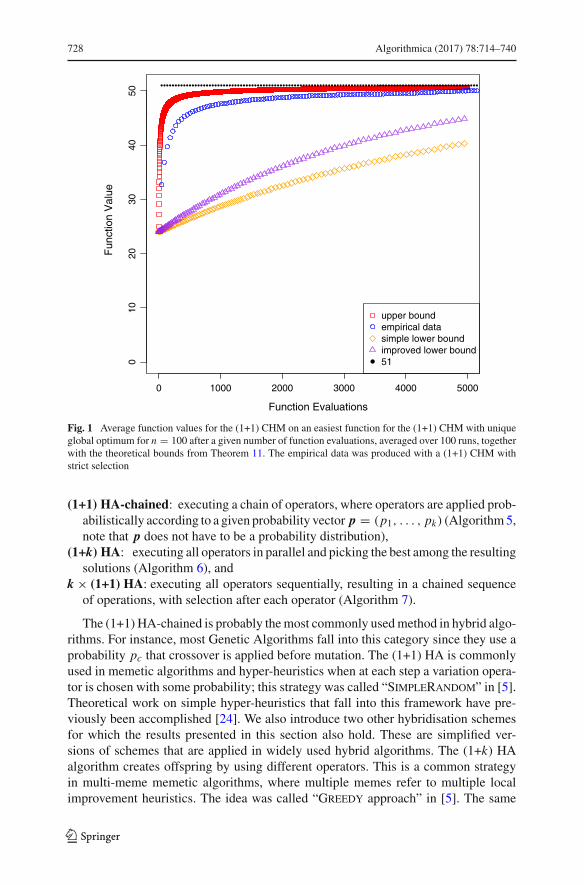
To obtain actual lower and upper bounds we use the lower and upper bounds for theinitial expected function value from Theorem 10. While the bounds from Theorem 11are not simple and in particular the upper bound is not even a closed form, we caneasily evaluate them numerically for reasonable values of n. In Fig. 1 we displaythem for n = 100 together with the maximal function value 51 and empirical resultsaveraged over 100 runs. We see that while the upper bound yields reasonable resultsboth lower bounds are rather weak.

5 Hybridising Operators

A popular approach in areas such as memetic algorithms [27] or hyper-heuristics [30]is to combine several operators in one algorithm. There are many ways of hybridisingalgorithms – here, we consider four different schemes of hybridisation that combine koperators.Given several (1+1) As, A1, · · · , Ak , the different hybridisations consideredare:

(1+1) HA: executing one operator chosen probabilistically according to a given prob-ability distribution p = (p1, . . . , pk) (Algorithm 4),

123

728 Algorithmica (2017) 78:714–740

0 1000 2000 3000 4000 5000

010

2030

4050

Function Evaluations

Fun

ctio

n V

alue

upper boundempirical datasimple lower boundimproved lower bound51

Fig. 1 Average function values for the (1+1) CHM on an easiest function for the (1+1) CHM with uniqueglobal optimum for n = 100 after a given number of function evaluations, averaged over 100 runs, togetherwith the theoretical bounds from Theorem 11. The empirical data was produced with a (1+1) CHM withstrict selection

(1+1) HA-chained: executing a chain of operators, where operators are applied prob-abilistically according to a given probability vector p = (p1, . . . , pk) (Algorithm5,note that p does not have to be a probability distribution),

(1+k) HA: executing all operators in parallel and picking the best among the resultingsolutions (Algorithm 6), and

k × (1+1) HA: executing all operators sequentially, resulting in a chained sequenceof operations, with selection after each operator (Algorithm 7).

The (1+1) HA-chained is probably themost commonly usedmethod in hybrid algo-rithms. For instance, most Genetic Algorithms fall into this category since they use aprobability pc that crossover is applied before mutation. The (1+1) HA is commonlyused in memetic algorithms and hyper-heuristics when at each step a variation opera-tor is chosen with some probability; this strategy was called “SimpleRandom” in [5].Theoretical work on simple hyper-heuristics that fall into this framework have pre-viously been accomplished [24]. We also introduce two other hybridisation schemesfor which the results presented in this section also hold. These are simplified ver-sions of schemes that are applied in widely used hybrid algorithms. The (1+k) HAalgorithm creates offspring by using different operators. This is a common strategyin multi-meme memetic algorithms, where multiple memes refer to multiple localimprovement heuristics. The idea was called “Greedy approach” in [5]. The same

123

Algorithmica (2017) 78:714–740 729

idea also appears in simple island models with heterogeneous islands, that is, eachisland consists of one individual and uses a different variation operator. A real-worldexample of where such a strategy is used (albeit with populations and added complex-ity) is theWegener system, a popular and effective algorithm in search-based softwaretesting, where different islands use standard bit mutations with different mutationrates [36]. The k×(1+1) HA is interesting as it has some resemblance to the recentlyintroduced (1+(λ,λ)) GA, since both use selection between the application of the oper-ators. However, the (1+(λ,λ)) GAdoes not fall exactlywithin the k×(1+1)HA scheme.In the former, if the final solution is worse than the initial one in the sequence, then theinitial solution is accepted for the next generation. On the other hand, the k×(1+1) HAalways accepts the last improving solution in the sequence.

Note that (1+1)HA-chained and k×(1+1)HAdiffer in the use of selection: the latterapplies selection after each operator, whereas the former only applies selection at theend of the generation. One generation of (1+k) HAmay be regarded as a derandomisedversion of (1+1) HA(1/k, . . . , 1/k) run for k generations. In the former all operatorsare executed once, whereas in the latter algorithm all operators are executed once inexpectation. The latter also admits non-uniform probabilities.

Algorithm 4 Hybrid algorithm (1+1) HA( p) (probabilistic choice of operator)1: input: fitness function f ;2: generate a solution x ;3: while the maximum value of f is not found do4: choose Ai with probability pi ;5: apply one iteration (mutation and selection) of Ai to generate y;6: update x with y if f (y) > f (x);7: end while8: output: the maximal value of f .

Algorithm 5 Hybrid algorithm (1+1) HA-chained( p) (probabilistic chain)1: input: fitness function f ;2: generate a solution x ;3: while the maximum value of f is not found do4: let y := x ;5: for i = 1, . . . , k do6: with probability pi update y by applying one iteration of Ai without selection;7: end for8: update x with y if f (y) > f (x);9: end while10: output: the maximal value of f .

Algorithm 6 Hybrid algorithm (1+k) HA (parallel operations)1: input: fitness function f ;2: generate a solution x ;3: while the maximum value of f is not found do4: for i = 1, . . . , k do5: apply one iteration (mutation and selection) of Ai to generate yi ;6: end for7: update x with a best search point from {y1, . . . , yk } if its fitness is larger than f (x);8: end while9: output: the maximal value of f .

123

730 Algorithmica (2017) 78:714–740

Algorithm 7 Hybrid algorithm k×(1+1) HA (sequential operations)1: input: fitness function f ;2: generate a solution x ;3: while the maximum value of f is not found do4: for i = 1, . . . , k do5: apply one iteration (mutation and selection) of Ai to generate y;6: update x with y if f (y) > f (x);7: end for8: end while9: output: the maximal value of f .

The B-cell algorithm (BCA) [23] is an example of an algorithm that uses both SBMand CHM considered in this paper. More specifically, it uses a population of searchpoints and creates λ clones for each of them. It then applies standard bit mutation to arandomly selected clone for each parent search point and subsequently applies CHMto all clones. This way one offspring of each parent is subject to a sequence of twomutations, first standard bit mutation and afterwards CHM. Jansen et al. [14] proposeda variant of the BCA that only uses CHM with constant probability 0 < p < 1(instead of p = 1) and were able to show significantly improved upper bounds onthe optimisation time for this algorithm on instances of the vertex cover problem.Considering the individuals that undergo both kinds of mutation (or a (1+1)-styleBCA), both these variants fit within the (1+1) HA-chained model of hybridisation(Algorithm 5). More precisely, for p = (p1, p2) with p1 the probability to executeSBM and p2 the probability to execute CHM, we have p1 = p2 = 1 for the originalBCA and constant p1 = 1 and 0 < p2 < 1 for the modified BCA in [14]. We remarkthat the improved results in [14] in fact hold as long as p1 = Ω (1).

In the following subsection we will first consider the general hybrid algorithmicframework and then specialise the results to the combination of CHM and SBM.

5.1 The Advantage of Hybridisation

The easiest functions for SBM and CHM areOneMax andMinBlocks, respectively.Before analysing hybrid algorithms using both operators, it is natural to consider theeffect of one operator on the easiest function for the other operator. It is well knownthat the (1+1) CHM needs (n2 log n) expected time on OneMax [17,21].

Here we consider the expected optimisation time of the (1+1) EA on MinBlocksand show that it is very inefficient.

Theorem 12 The expected optimisation time of the (1+1) EA with strict or non-strictselection on MinBlocks is at least nn/2.

Proof The function MinBlocks has the following property: for all search pointsexcept for 0n and 1n , the number of 0-blocks equals the number of 1-blocks. Noticethat inverting all bits in a bit string turns all 0-blocks into 1-blocks and vice versa.Hence for all x /∈ {0n, 1n} we have MinBlocks(x) = MinBlocks(x).

Let x0, x1, . . . be the trajectory of the (1+1) EA and T ∈ N0 be the first hittingtime of a search point in {0n, 1n}. Since x0, x1, . . . , xT has the same probability as

123

Algorithmica (2017) 78:714–740 731

x0, x1, . . . , xT and xT ∈ {0n, 1n}, we have Pr (xT = 0n) = 1/2. In this case the onlyaccepted search point is the global optimum 1n , for which all bits have to be flippedin one mutation. This has probability n−n and expected waiting time nn . Combinedwith the probability of reaching this state, the expected optimisation time is at leastT + nn/2 ≥ nn/2.

Note that the expected optimisation time of the (1+1) EA on MinBlocks is onlyby a factor of at most 2 smaller than the expected optimisation time of the (1+1) EAon its hardest function, Trap, which is almost nn [9].

Using multiple operators, the hope is that the advantages of each operator are com-bined. However, this is not always true: new operators can make a hybrid algorithmfollow an entirely different search trajectory and lead to drastically increased optimi-sation times. This behaviour was demonstrated for memetic algorithms [31] as wellas for standard bit mutations cycling between different mutation rates [15] and forpopulation based EAs where the mutation rate of each individual depends on its rankin the population [28].

We show that such effects cannot occur when dealing with easiest functions. If fis an easiest function for A which is a (1+1) A, then Theorem 13 stated below allowsto transfer an upper bound on the expected optimisation time of A to the four hybridalgorithms.

Theorem 13 If A1, . . . , Ak are (1+1) A’s with strict or non-strict selection, startingin x0, and f is an easiest function for Ai , then the expected hitting time of (1+1) HA( p)on f , for a probability distribution p = (p1, . . . , pk), is bounded from above by

1

pi· T (Ai , f, x0).

For any probability vector p = (p1, . . . , pk) with pi > 0 and p j < 1 for all j �= i ,the expected hitting time of (1+1) HA-chained( p) on f is bounded from above by

1

pi · ∏j �=i (1 − p j )

· T (Ai , f, x0).

Moreover, the expected hitting time of (1+k) HA and k×(1+1) HA is bounded fromabove by

k · T (Ai , f, x0).

Proof We follow the analysis in [10, Section III] and perform a drift analysis, choosingthe runtime T (Ai , f, x) as the drift function:

d(x) = T (Ai , f, x).

Define ΔA j (x) = E ((d(x) − d(y))) as the drift of Algorithm A j , given that y wascreated by applying A j to x . The drift of the hybrid algorithm (1+1) HA( p) is

123

732 Algorithmica (2017) 78:714–740

Δ(1+1) H A(x) =k∑

i=1

piΔAi (x).

We apply Lemma 3 in [10] to estimate ΔAi . For any non-optimal point x , let y be itschild, then the drift of algorithm Ai satisfies

ΔAi (x) = E(d(x) − d(y)) = 1 (3)

following from the definition of d(x) = T (Ai , f, x). We further claim that no operatorinduces a negative drift. Given any two non-optimal points x and y, then when usingstrict selection, according to the monotonically decreasing condition d(x) < d(y)implies f (x) > f (y). By contraposition, we get

f (y) ≥ f (x) ⇒ d(y) ≤ d(x). (4)

When using non-strict selection, the strictly monotonically decreasing conditionimplies f (y) ≥ f (x) ⇔ d(y) ≤ d(x), which implies (4) as well. Since all algo-rithms A1, . . . , Ak adopt elitist selection, the distance cannot increase, regardless ofwhich operator is chosen. Hence ΔA j (x) ≥ 0 for all j and

Δ(1+1) H A(x) ≥ piΔAi (x) = pi .

Using the additive drift theorem, Theorem 2, the expected hitting time of (1+1) HA( p)on f is at most

d(x0)

pi= T (Ai , f, x0)

pi.

For (1+1) HA-chained we observe that the algorithm executes only Ai and none ofthe other operators with probability pi · ∏ j �=i (1− p j ). In all other cases the distancecannot increase (by (4)). Hence by the same arguments as above, the expected hittingtime is bounded by

1

pi · ∏j �=i (1 − p j )

· T (Ai , f, x0).

The statement on (1 + k) HA follows from similar arguments. Let x1, . . . , xk be thesearch points created using A1, . . . , Ak , respectively. Let x∗ be the best amongst these,selected for survival. Then f (x∗) ≥ f (xi ), and by (4), d(x∗) ≤ d(xi ). Hence for allnon-optimal x ,

Δ(1+k) H A(x) ≥ ΔAi (x) = 1.

Additive drift from Theorem 2 then yields an upper bound on the expected time of(1+k) HA of k ·T (Ai , f, x0), the factor k accounting for executing k operations in onegeneration.

123

Algorithmica (2017) 78:714–740 733

Finally, for k×(1+1) HA, let x1, . . . , xk be the offspring created in the sequence ofoperations and note that xk is taken over for the next generation. We have f (xi−1) ≥· · · ≥ f (x1) ≥ f (x) and thus d(xi−1) ≤ d(x) by (4). Along with ΔAi (x) = 1 for allnon-optimal x and f (xk) ≥ f (xi ) implying d(xk) ≤ d(xi ), we get

Δk×(1+1) H A(x) ≥ ΔAi (x) = 1

and an upper bound of k · T (Ai , f, x0) as for (1+k) HA. Using Theorem 13 as well as Theorem 9, we get the following corollary concerning

the SBM and CHM operators.

Corollary 14 Consider thehybrid algorithms (1+1)HA( p)and (1+1)HA-chained( p)for p = (p1, p2) with constant p1, p2 > 0, (1+2) HA, and 2×(1+1) HA, all based ona (1+1) algorithm A1 using SBM and another (1+1) algorithm A2 using CHM; A1and A2 both using strict or non-strict selection. Then the expected optimisation time ofall these hybrids onOneMax andMinBlocks is O(n log n) and O(n2), respectively.

All hybrid algorithms are hence able to combine the advantages of both operators onthe two easiest functions for its two operators. This is particularly true for the modified(1+1)-style BCA [14] with constant 0 < p1, p2 < 1 discussed at the beginning ofSect. 5.

5.2 Weighted Combinations of OneMax and MINBLOCKS

In the previous subsection it was proven that the four different hybrid schemes(1+1) HA( p) for p = (p1, p2) with constant p1, p2 > 0, (1+1) HA-chained,(1+2) HA, and 2×(1+1) HA, using SBM and CHM as operators are all efficientfor OneMax and MinBlocks. In particular, even though SBMs alone exhibit verypoor performance onMinBlocks, hybrid algorithms using CHMwith arbitrarily lowconstant probability along with SBM are efficient. In this subsection we investigatethe performance of the two operators on “hybrid” functions where the fitness dependson both the number of ones and the number of blocks.

To this end, we perform experiments concentrating on different instantiations ofAlgorithm (1+1)HA( p) for p = (p, 1−p)with various values of p and strict selectionand investigate its performance on a function consisting of weighted combinations ofOneMax and MinBlocks. To be more precise we consider the function

fw(x) = w · OneMax(x) + (1 − w) · MinBlocks(x)

with w ∈ {0, 0.1, 0.2, . . . , 1.0} ∪ {1/n, 1/n2} and the (1+1) HA(p, 1− p) where weexecute CHM with probability p and standard bit mutations with probability 1 − pwith p ∈ {0, 0.1, 0.2, . . . , 1.0} ∪ {1/n, 1/n2}. Note, that for p = 0 and w = 0 weonly use standard bit mutations on pure MinBlocks and thus, the optimisation timeis exponential (Theorem 12). Similarly, we have an optimisation time of (n log n)

for p = 0 and w = 1 (standard bit mutations on pure OneMax [9]), (n2 log n

)

123

734 Algorithmica (2017) 78:714–740

for p = 1 and w = 1 (CHM on pure OneMax [17]) and (n2

)for p = 1 and

w = 0 (CHM on pure MinBlocks, Theorem 9). We are particularly interested inintermediate values of p and w and their influence on the optimisation time.

We perform 10,000 runs for each of the above pairs of settings for n = 100 anddepict the average optimisation times in Fig. 2. Figure 2a shows a comparison of theoptimisation times of different resulting algorithms (1+1) HA(p, 1 − p) dependingon w while Fig. 2b depicts the results for different functions over the parameter p ofthe hybrid algorithm. Note, that for the sake of recognisability we only depict a subsetof the curves in both figures while on each curve we present all available data points.We additionally perform Wilcoxon signed rank tests to assess whether the observeddifferences in the optimisation times are statistically significant. Fixing a value for w

(Fig. 2a) we perform tests for all pairs of algorithms and the 10,000 optimisation timesmeasured for each setting. Similarly, fixing a value for p (Fig. 2b) we perform testsfor all pairs of functions. We perform Holm-Bonferroni correction to account for thelarge number of tests we execute.

We observe that for allw > 0, the runtime gets smaller as p decreases (Fig. 2a). Alldifferences are statistically significant at confidence level 0.05 with the exception ofp = 0 and p = 1/n2 for all values of w and p = 0, p = 1/n2, p = 1/n and p = 0.1for most w ∈ {0.1, 0.2, 0.3, 0.4}. From Fig. 2b we can also see that the (1+1) HA( p)with constant p < 0.7 appears to be faster on functions fw with constant w > 0 (i. e.,with constant OneMax fraction) while using a larger p (i. e., performing CHM moreoften) pays off for w = o (1). Differences are statistically significant at confidencelevel 0.05 with the exception of most results for p = 0.7 and p = 0.8, w = 1/n andw = 1/n2 for all p ≤ 0.8, w ≥ 0.6 for all p, w ≥ 0.3 for all p ≥ 0.5, and w ≤ 0.2for w = 0, w = 1/n2 and w = 1/n.

We can see from the experiments in Fig. 2 that the case w = 0 is very differentfrom runs with w > 0. Recall that w = 0 means that the algorithm is confrontedwith MinBlocks and that w > 0 implies that we add w · OneMax to the functionvalue (while, at the same time, reducing the function value by w · MinBlocks). Theaddition ofw ·OneMaxwith an arbitrarily smallw > 0 introduces a ‘search gradient’in the fitness landscape: the algorithm is encouraged to increase the number of 1-bitsby a small increase in fitness (at least as long as this trend is not counteracted by anincrease in the number of blocks). The effect is most pronounced for p = 0, i. e., forthe (1+1) EA where the expected optimisation time is exponential for MinBlocksand becomes manageable as soon as the OneMax-component introduces a ‘searchgradient’. In a different context, the same effect has been discussed and analysed usingdifferent example functions [16].

5.3 On the Easiest Function for Hybrid Algorithms

In the previous subsection itwas shownexperimentally that as soon as a smallOneMaxcomponent comes into play, the function fw becomes easy for the (1+1) HA(p,1− p)usingSBMandCHMindependent of the value of p. Nevertheless, in this subsectionweshow that fw, for any value ofw, is not an easiest function for the (1+1) HA(p,1− p).In particular, we will set p = 1/2 and show that the easiest function for the hybrid

123

Algorithmica (2017) 78:714–740 735

●

●● ● ● ● ● ● ● ● ● ● ●

●

●●● ● ● ● ● ● ● ● ● ●

1e+02

1e+04

1e+06

1e+08

1e+10

0.00 0.25 0.50 0.75 1.00w

Func

tion

Eva

luat

ions

(log

scal

e)

Algorithms: p= ● ●0.0 1/n^2 1/n 0.1 0.3 0.5 0.7 0.9 1.0(a)

●●●●●●

●

●

●

●

●

●

●

●

●

●

●●

●●●

● ●

●●

●

1e+03

1e+04

1e+05

1e+06

0.00 0.25 0.50 0.75 1.00p

Func

tion

Eva

luat

ions

(log

scal

e)

Functions: w= ● ●0.0 1/n^2 1/n 0.1 0.3 0.5 0.7 0.9 1.0(b)

Fig. 2 Results of the experiments: Average optimisation times over 10,000 independent runs for each pairof p and w for n = 100. The empirical data was produced with a (1+1) HA(p, 1− p) with strict selection.a Results for different algorithms (1+1) HA(p, 1 − p) over values for w. b Results for different functionsfw over values for p

123

736 Algorithmica (2017) 78:714–740

algorithm (1+1) HA(1/2,1/2) using SBM and CHM, and strict selection, is morecomplex than a mere weighted combination fw of the two easiest functions for bothoperators.

He et al. [10] explain how an easiest function can be computed. We constructEasiestHybridp, an easiest fitness function for the hybrid algorithm (1+1) HA(p,1−p) from Corollary 14 by implementing their construction procedure and performingthe necessary computations numerically. Clearly, this is computationally feasible onlyfor small values of n. Using the unique global optimum as a starting point and levelL0 we can compute the next level of search points with next best and equal fitness bycomputing for each search point which does not yet have a level the expected timeneeded to reach L0 either directly or via a mutation to a search point that already has alevel. Search points with minimal time in this round make up the next level. Note thatthis is actually Dijkstra’s algorithm for computing shortest paths (see, e. g., [3]). Alsonote that the numerical computation of the actual expected waiting times is easy sincethe exact transition probabilities for mutations leading from one bit string to anotherare all known and waiting times are all simply geometrically distributed.

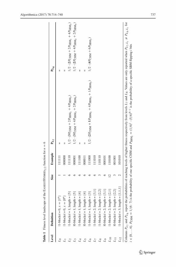
The easiest function for the (1+1) CHM is composed of �n/2 + 2 different fitnesslevels, L0, . . . , L�n/2 +1, defined by a number of 1-blocks (i. e., L0 = {1n}, L1 = {0n},Li = {x ∈ {0, 1}n | x contains i − 1 different 1-blocks} for each i ∈ {2, . . . , �n/2 +1}). On the other hand, the fitness level set of the easiest function for the (1+1) EA (i. e.,OneMax) has n + 1 different levels defined by a number of 1-bits (i. e., Li = {x ∈{0, 1}n | x contains n − i 1-bits} for each i ∈ {0, . . . , n}). If EasiestHybridp was amere weighted combination of OneMax and MinBlocks, its fitness levels would bedefined by a combination of a number of 1-blocks and a number of 1-bits. This wouldhappen because individuals that have the same number of 1-bits and the same numberof 1-blocks would have exactly the same fitness. Also, the product between the numberof levels of the easiest functions for each operator, (�n/2 + 2) · (n + 1), would bean upper bound on the number of levels for EasiestHybridp. In the following weshow that neither of these two considerations are true and that the fitness levels ofthe easiest function for the hybrid algorithm are more complicated. In particular, bitstrings having in common the same number of 1-blocks and the same number of 1-bitscan belong to different fitness levels of EasiestHybridp. Rather, the length of theblocks comes into play to define the fitness levels even though such a feature does notdefine the levels of either OneMax or MinBlocks.

We consider Algorithm (1+1) HA(p,1 − p) which at each step executes eitheran SBM or a CHM with probability p = 1/2 and report in Table 1 the differentfitness levels L0, . . . , L12 of EasiestHybrid1/2 when n = 6. From the table it canbe noticed that both levels L7 and L8 contain bit strings with two 1-blocks and four1-bits. However, the lengths of the two 1-blocks are different (i. e., three and one for L7and two and two for L8). The reason why levels L7 and L8 are distinct is highlightedin the last two columns of Table 1, which report the probabilities of reaching levels ofhigher fitness, respectively from levels L7 and L8. For any point of the search spacebelonging to level L7 there are three different CHMs leading to points in L2 and L3while there are only two CHMs from points in L8. These extra CHMs lead to highertransition probabilities, hence lower runtimes, to reach levels L2 and L3 from L7,compared to L8. Also the probability of reaching level L6 is higher from L7, mainly

123

Algorithmica (2017) 78:714–740 737

Table1

Fitnesslevellandscape

oftheEasiestH

ybr

id1/2functio

nforn

=6

Level

Defi

nition

Size

Exa

mple

PL7

PL8

L0

|1-blocks|=0,

x=

{1n}

111

1111

==

L1

|1-blocks|=0,

x=

{0n}

100

0000

==

L2

|1-blocks|=1;

leng

th={5}

611

1110

1/2

·(3P C

HM

+2P S

BM

1+

4P S

BM

3)

1/2

·(2P C

HM

+2P S

BM

1+

4P S

BM

3)

L3

|0-blocks|=1;

leng

th={5}

600

0001

1/2

·(3P C

HM

+4P S

BM

3+

2P S

BM

5)

1/2

·(2P C

HM

+4P S

BM

3+

2P S

BM

5)

L4

|1-blocks|=1;

leng

th={4}

611

1100

==

L5

|0-blocks|=1;

leng

th={4}

600

0011

==

L6

|1-blocks|=1;

leng

th={3}

611

1000

1/2

·(2P C

HM

+1P S

BM

1+

4P S

BM

3+

1P S

BM

5)

1/2

·(4P C

HM

+6P S

BM

3)

L7

|1-blocks|=2;

leng

th={3,1}

611

1010

L8

|1-blocks|=2;

leng

th={2,2}

311

0110

L9

|0-blocks|=2;

leng

th={3,1}

600

0101

L10

|1-blocks|=2;

leng

th={2,1}

1211

0100

L11

|0-blocks|=2;

leng

th={2,2}

300

1001

L12

|1-blocks|=3;

leng

th={1,1,1}

210

1010

Colum

nsPL7andPL8repo

rttheprob

abilitie

sof

reaching

levelsof

high

erfitness

respectiv

elyfrom

levelsL7andL8.V

aluesareonly

reported

whenPL7,L

i�=

PL8,L

ifor

i∈{

0,..

.6}.P C

HM

=1/

(6·7

)istheprobability

ofonespecificCHM

andP S

BM

i=

(1/6)

i·(5

/6)

6−iistheprob

ability

ofaspecificSB

Mflipp

ingibits

123

738 Algorithmica (2017) 78:714–740

because the level may be reached by flipping only one bit while at least three bits needto be flipped for bit strings in L8. Since the transition probabilities to the remaininglevels of higher fitness are the same, the expected runtime from L7 is lower than thatfrom L8, explaining why the two levels are distinct (recall that, by construction, thelevels are ordered according to increasing expected runtimes).

Concerning the number of different fitness levels, these increase as the problemsize n increases. Already for n = 10 EasiestHybrid1/2 has 78 different levels, morethan the product of the number of OneMax and MinBlocks levels for n = 10 (i. e.66). It is indeed the increase in number of fitness levels as n grows that makes it hardto give a precise definition of the EasiestHybrid1/2 function. We leave this as anopen problem for future work.

6 Conclusions

We have extended the analysis of easiest function classes from standard bit mutationsto the contiguous somatic hypermutation (CHM) operator used in artificial immunesystems. Albeit the recent advances in their theoretical foundations [21,29,35] no suchresults were available concerning artificial immune system operators. With the run-time and fixed budget analyses of the (1+1) CHM onMinBlocks, the correspondingeasiest function, we established a lower bound on the (1+1) CHM’s performance onany function. We also showed that MinBlocks is exponentially hard for the standard(1+1) EA, complementing the known result that the (1+1) CHM performs asymptoti-cally worse by a factor of(n) compared to the (1+1) EA onOneMax. Furthermore,we proved that several hybrid algorithms combining the (1+1) CHM and the (1+1) EAsolve both MinBlocks and OneMax only at a constant factor slower than the purealgorithms.

Experimental work revealed that a fitness function consisting of a weighted com-bination of MinBlocks and OneMax is easy to optimise for both pure operatorsand hybrid variants even when the OneMax weight component is very small. Nev-ertheless, after providing the exact fitness landscape of the easiest function for the(1+1) HA(1/2,1/2), EasiestHybrid1/2 for small instance sizes, we observed thatits structure is more complex than a simple weighted combination of OneMax andMinBlocks.We leave constructing and analysing easiest functions for other operatorsthat fit the (1+1) A scheme for future work. Similarly, the question about the easiestfunctions for different schemes of hybridisation remains open.

Acknowledgements The research leading to these results has received funding from the European UnionSeventh Framework Programme (FP7/2007-2013) under Grant Agreement No. 618091 (SAGE) and by theEPSRC under Grant Agreement No. EP/M004252/1. We thank the anonymous reviewers of this manuscriptand the previous GECCO 2015 paper for their very useful and constructive comments.

Open Access This article is distributed under the terms of the Creative Commons Attribution 4.0 Interna-tional License (http://creativecommons.org/licenses/by/4.0/), which permits unrestricted use, distribution,and reproduction in any medium, provided you give appropriate credit to the original author(s) and thesource, provide a link to the Creative Commons license, and indicate if changes were made.

123

Algorithmica (2017) 78:714–740 739

References

1. Alanazi, F., Lehre, P.K.: Runtime analysis of selection hyper-heuristics with classical learning mech-anisms. In: Proceedings of the IEEE Congress on Evolutionary Computation (CEC 2014), pp.2515–2523. IEEE (2014)

2. Clark, E., Hone, A., Timmis, J.: A markov chain model of the B-cell algorithm. In: Proceedings of theInternational Conference on Artificial Immune Systems (ICARIS 2005), LNCS 3627, pp. 318–330.Springer (2005)

3. Cormen, T.H., Leiserson, C.E., Rivest, R.L., Stein, C.: Introduction to Algorithms. MIT Press, London(2001)

4. Corus, D., He, J., Jansen, T., Oliveto, P.S., Sudholt, D., Zarges, C.: On easiest functions for somaticcontiguous hypermutations and standard bitmutations. In: Proceedings of theGenetic andEvolutionaryComputation Conference (GECCO 2015), pp. 1399–1406. ACM (2015)

5. Cowling, P., Kendall, G., Soubeiga, E.: A hyperheuristic approach to scheduling a sales summit. In:Burke, E., Erben, W. (eds) Proceedings of the Third International Conference on Practice and Theoryof Automated Timetabling (PATAT 2000), pp. 176–190. Springer (2001)

6. de Castro, L.N., Timmis, J.: Artificial Immune Systems: ANewComputational Intelligence Approach.Springer, Berlin (2002)

7. Doerr, B.,Doerr, C., Ebel, F.: Fromblack-box complexity to designing newgenetic algorithms. Theoret.Comput. Sci. 567, 87–104 (2015)

8. Doerr, B., Johannsen, D., Winzen, C.: Drift analysis and linear functions revisited. In: Proceedings ofthe IEEE Congress on Evolutionary Computation (CEC 2010), pp. 1967–1974 (2010)

9. Droste, S., Jansen, T., Wegener, I.: On the analysis of the (1+1) evolutionary algorithm. Theoret.Comput. Sci. 276, 51–81 (2002)

10. He, J., Chen, T., Yao, X.: On the easiest and hardest fitness functions. IEEE Trans. Evol. Comput.19(2), 295–305 (2015)

11. He, J., Yao, X.: A study of drift analysis for estimating computation time of evolutionary algorithms.Nat. Comput. 3(1), 21–35 (2004)

12. Jansen, T.: Analyzing Evolutionary Algorithms: The Computer Science Perspective. Springer, Berlin(2013)

13. Jansen, T., De Jong, K.A., Wegener, I.: On the choice of the offspring population size in evolutionaryalgorithms. Evol. Comput. 13(4), 413–440 (2005)

14. Jansen, T., Oliveto, P.S., Zarges, C.: On the analysis of the immune-inspired B-cell algorithm for thevertex cover problem. In: Proceedings of the International Conference on Artificial Immune Systems(ICARIS 2011), LNCS 6825, pp. 117–131. Springer (2011)

15. Jansen, T., Wegener, I.: On the choice of the mutation probability for the (1+1) EA. In: Proceedings ofthe 6th International Conference on Parallel Problem Solving from Nature (PPSN 2000), LNCS 1917,pp. 89–98. Springer (2000)

16. Jansen, T., Wiegand, R.P.: The cooperative coevolutionary (1+1) EA. Evol. Comput. 12(4), 405–434(2004)

17. Jansen, T., Zarges, C.: Analyzing different variants of immune inspired somatic contiguous hypermu-tations. Theoret. Comput. Sci. 412(6), 517–533 (2011)

18. Jansen, T., Zarges, C.: Computing longest common subsequences with the B-cell algorithm. In: Pro-ceedings of the International Conference on Artificial Immune Systems (ICARIS 2012), LNCS 7597,pp. 111–124. Springer (2012)

19. Jansen, T., Zarges, C.: Fixed budget computations: a different perspective on run time analysis. In:Proceedings of the Genetic and Evolutionary Computation Conference (GECCO 2012), pp. 1325–1332. ACM (2012)

20. Jansen, T., Zarges, C.: Performance analysis of randomised search heuristics operating with a fixedbudget. Theoret. Comput. Sci. 545, 39–58 (2014)

21. Jansen, T., Zarges, C.: Reevaluating immune-inspired hypermutations using the fixed budget perspec-tive. IEEE Trans. Evol. Comput. 18(5), 674–688 (2014)

22. Jansen, T., Zarges, C.: Analysis of randomised search heuristics for dynamic optimisation. Evol. Com-putation. 23(4), 513–541 (2015)

23. Kelsey, J., Timmis, J.: Immune inspired somatic contiguous hypermutations for function optimisation.In: Proceedings of the Genetic and Evolutionary Computation Conference (GECCO 2003). LNCS2723, pp. 207–218. Springer (2003)

123

740 Algorithmica (2017) 78:714–740

24. Lehre, P.K., Özcan, E.: A runtime analysis of simple hyper-heuristics: to mix or not to mix operators.In: Proceedings of the Twelfth workshop on Foundations of Genetic Algorithms (FOGA 2013), pp.97–104. ACM (2013)

25. Lehre, P.K., Witt, C.: General drift analysis with tail bounds. CoRR, abs/1307.2559 (2013)26. Lengler, J., Spooner, N.: Fixed budget performance of the (1+1) EA on linear functions. In: Proceedings

of the 2015 ACMConference on Foundations of Genetic Algorithms (FOGA 2015), pp. 52–61 (2015)27. Neri, F., Cotta, C., Moscato, P. (eds.): Handbook of Memetic Algorithms. Springer, Berlin (2013)28. Oliveto, P.S., Lehre, P.K., Neumann, F.: Theoretical analysis of rank-based mutation—combining

exploration and exploitation. In: Proceedings of the IEEE Congress on Evolutionary Computation(CEC 2009), pp. 1455–1462 (2009)

29. Oliveto, P.S., Sudholt, D.: On the runtime analysis of stochastic ageing mechanisms. In: Proceedingsof the Genetic and Evolutionary Computation Conference (GECCO 2014), pp. 113–120. ACM (2014)

30. Ross, P.: Hyper-heuristics. In: Burke, E.K., Kendall, G. (eds.) Search Methodologies, pp. 611–638.Springer, Berlin (2014)

31. Sudholt, D.: The impact of parametrization in memetic evolutionary algorithms. Theoret. Comput. Sci.410(26), 2511–2528 (2009)

32. Sudholt, D.: Hybridizing evolutionary algorithmswith variable-depth search to overcome local optima.Algorithmica 59(3), 343–368 (2011)

33. Sudholt, D.: A new method for lower bounds on the running time of evolutionary algorithms. IEEETrans. Evol. Comput. 17(3), 418–435 (2013)

34. Sudholt, D., Zarges, C.: Analysis of an iterated local search algorithm for vertex coloring. In: Pro-ceedings of the 21st International Symposium on Algorithms and Computation (ISAAC 2010), LNCS6506, pp. 340–352. Springer (2010)

35. Timmis, J., Hone, A., Stibor, T., Clark, E.: Theoretical advances in artificial immune systems. Theoret.Comput. Sci. 403(1), 11–32 (2008)

36. Wegener, J., Baresel, A., Sthamer, H.: Evolutionary test environment for automatic structural testing.Inf. Softw. Technol. 43(14) 841–854 (2001)

37. Witt, C.: Tight bounds on the optimization time of a randomized search heuristic on linear functions.Comb. Probab. Comput. 22(2), 294–318 (2013)

123