On Edge Detection on Surfaces

Michael KolomenkinTechnion

michkol@tx.technion.ac.il

Ilan ShimshoniUniversity of Haifa

ishimshoni@mis.haifa.ac.il

Ayellet TalTechnion

ayellet@ee.technion.ac.il

Abstract

Edge detection in images has been a fundamental prob-lem in computer vision from its early days. Edge detectionon surfaces, on the other hand, has received much less at-tention. The most common edges on surfaces are ridgesand valleys, used for processing range images in computervision, as well as for non-photorealistic rendering in com-puter graphics. We propose a new type of edges on surfaces,termed relief edges. Intuitively, the surface can be consid-ered as an unknown smooth manifold, on top of which alocal height image is placed. Relief edges are the edges ofthis local image. We show how to compute these edges fromthe local differential geometric surface properties, by fittinga local edge model to the surface. We also show how theunderlying manifold and the local images can be roughlyapproximated and exploited in the edge detection process.Last but not least, we demonstrate the application of reliefedges to artifact illustration in archaeology.

1. IntroductionEdges in images provide low-level cues, which can be

utilized in higher level processes, such as object detection,recognition, and classification, as well as motion detection,image matching, and tracking [3, 18]. They are more re-silient to image formation parameters than the image in-tensity values, while containing less information than thewhole image.

Edges on surfaces can be used in a similar way [2, 9].While edges in images can have a variety of causes, such asdepth discontinuities, textures, shadows, and other lightingeffects that might hinder their use for higher level processes,edges on surfaces are the outcome of the surface geometryonly (see Figure 1). This paper focuses on the problem ofaccurately detecting edges on surfaces.

Many of the existing algorithms detect ridges and val-leys, which are the extrema of principal curvatures [12, 19,22]. Other types of curves are parabolic curves, which par-tition the surface into hyperbolic and elliptic regions, andzero-mean curvature curves, which classify sub-surfaces

(a) The scanned object (b) Ridges & valleys

(c) Demarcating curves (d) Relief edges

Figure 1. A seal from the early Iron Age, 11th century BCE

into concave and convex shapes [13]. They correspond tothe zeros of the Gaussian and mean curvature, respectively.Finally, demarcating curves are the zero-crossings of thecurvature in the curvature gradient direction [14]. Whileportraying important object properties, the aforementionedcurves sometimes fail to capture relevant features, such asweak edges, highly curved edges, and noisy surfaces. Asshown in [5], no specific curve fits all applications.

This paper proposes a novel type of surface edges,termed relief edges, which addresses these limitations. Con-sider a surface as an unknown smooth manifold (base), ontop of which a local height function is defined (e.g., a re-lief). The function can be considered locally as a standardimage defined on the tangent plane of the base. Relief edgesare the edges of this local image, i.e., a surface point p is arelief edge point if it is an edge point of this image.

We demonstrate that relief edges are smoother and moreaccurate than the other types of curves. They are better

1

suited for certain surfaces, such as reliefs prevalent in ar-chaeological artifacts.

The main contributions of the paper is thus threefold.First, we extend the definition of edges from functions ona plane to functions on an unknown manifold. Second, wedescribe an algorithm that extracts these edges. Finally, wedemonstrate the utility of these edges in archaeological ar-tifact illustration.

Algorithm overview: Relief edges are defined as the zerocrossings of the normal curvature in the direction perpen-dicular to the edge. Initially, the edge direction is estimatedfor every point by fitting a step edge model to the surface.Given the edge directions, the precise edge localization isobtained (Section 3).

The quality of the estimation of the edge directions isfurther improved (Section 4). First, a rough estimation ofthe base normal is employed to limit the range of possibleedge directions. Second, the edge directions are smoothed,while maintaining the properties of relief edges.

2. Related workThe paper proposes an extension of edge detection in im-

ages to arbitrary 2D surfaces. Hence, this section presentsrelated work both on images and on surfaces. It does notdescribe volumetric edges [26] that are mere extensions of2D edges to a higher dimension.

Edge detection in images: Edge detection has been ex-tensively investigated [8]. Our work is most closely relatedto gradient-based edge detection, which can be generallyclassified into two classes.

The first class defines edges as the maximum of asmoothed first derivative or zero crossings of a smoothedsecond derivative. These methods differ in the manner inwhich they smooth and the way the derivatives are calcu-lated. Examples include the maximum of the derivative ofthe Gaussian filter [4], the zero crossings of the Laplacianof the Gaussian [16], and the cubic spline filter [24].

Other methods attempt to implicitly fit the data to anedge model, such as a parametric-feature model [1] or a 1Dpolynomial [20]. The fitting determines both the orientationand the strength of the edge. These algorithms strongly relyon the edge model and thus might fail when the underlyingassumption of the edge is unsuitable.

Our approach most resembles [17], which combines bothtypes of edge detection algorithms. Canny edge detection isused for the initial edge estimation, followed by verificationthat is based on the correlation of the data with an edge tem-plate. This significantly increases the ability of the detectorto eliminate spurious edges and deal with weak edges.

Edge detection on surfaces: There are two classes ofedges on surfaces. The first includes ridges and val-

leys [12, 19, 22], which are the loci of points at whichthe curvature obtains extrema along the principal direction.They occur at surface normal discontinuities. Ridges andvalleys portray important object properties. However, illus-trating the object only by valleys (or ridges) is often insuffi-cient, since they do not always convey its structure. Draw-ing both will overload the image with too many lines. Itshould be noted that relief edges do not compete with ridgesand valleys, but rather complement them, since they portraylocations with different geometric properties.

The second class includes curves that are defined as thezero crossings of some function of curvature. Examplesinclude parabolic lines (zeros of Gaussian curvature) [13],curves of zero-mean curvature [13], and demarcating curves(zeros of the normal curvature in the curvature gradient di-rection) [14]. Parabolic curves are demonstrated to be noisyand unreliable [6, 14]. The curves of zero-mean curvaturedepend on the curvatures both along the edge and in the di-rection perpendicular to it; hence their error is high whenthe curvature in the edge direction is large. Both types ofcurves are isotropic operators and suffer from similar flawsas isotropic edges in images (e.g., Laplacian), such as poorbehavior at corners and inexact edge localization [8]. De-marcating curves might be noisy when the curvature alongthe edge varies. The relief edges proposed in this paper be-long to this class and address these problems.

Other kinds of curves are view dependent, i.e., theychange when the viewpoint changes [6, 11, 25]. Thesecurves are often aesthetically pleasing and thus are applica-ble for non-photorealistic rendering in computer graphics.

3. Relief edgesGiven a surface S(u, v) : R2 → R3, we assume that it

consists of a smooth base surface B(u, v) : R2 → R3 and afunction (local image) I(u, v) : R2 → R defined on B:

S(u, v) = B(u, v) + n(u, v)I(u, v), (1)

where u and v are the coordinates of a planar parametriza-tion and n(u, v) : R2 → S2 is the normal of B (S2 is theunit sphere). We assume that B is locally a manifold andthat its curvature has a smaller value than the curvature of I(Figure 2). The decoupling of S into B and I is unknown.Note that in the special case of an image, B is the imageplane, n(u, v) is constant, and I is the image intensity.

The goal is to detect edges on S that correspond to edgeson the local images I . We consider the common definitionof edges in images, as points at which the derivative obtainsa maximum in the gradient direction. We will show that theedges can be detected without accurately estimating B orits normal n – a rough estimate suffices.

In the following we first provide the necessary mathe-matical background and then describe the computation ofthe relief edges.

Figure 2. The surface S (magenta) is composed of a smooth baseB (black) and a function I (blue). Function I at point p can belocally viewed as an image defined on the tangent plane (orange)of the base. Point p is a relief edge point if it is an edge point ofthis image. The normal np (brown) is the normal of S and np

(green) is the normal of B corresponding to p.

3.1. Background

Before defining the curves, we review some definitionsin differential geometry [7]. The normal section of a surfaceat a point p in a tangent direction v is the intersection of thesurface with the plane defined by v and the normal to thesurface at p. The normal curvature at point p in directionv is the curvature of the normal section at p.

For a smooth surface, the normal curvature in directionv is

κ(v) = vT IIv. (2)

The symmetric matrix II is the second fundamental form:

II =[κ1 00 κ2

], (3)

where κ1 and κ2 are the principal curvatures.The derivatives of the curvature are defined by a 2×2×2

tensor with four unique numbers:

C = (∂uII; ∂vII) =[(

a1 a2

a2 a3

);(a2 a3

a3 a4

)],

(4)where ∂u and ∂v are the derivatives along the principal di-rections. Multiplying C from its three sides by a directionvector v, Cijkvivjvk gives a scalar, which is the derivativein direction v of the curvature in this direction.

The Monge form is a polynomial approximation of a sur-face S on the tangent plane at a given point, expressed as:

S(v) =12vT IIv +

12Cijkvivjvk = (5)

12 (κ1u

2 + κ2v2) + 1

6 (a1u3 + 3a2u

2v + 3a3uv2 + a4v

3),

where u and v are the coordinates of v in the princi-pal directions. We will be using the Monge form to lo-cally estimate the surface, utilizing the state-of-the-art tech-niques developed for estimating the curvature and its deriva-tive [10, 15, 23].

3.2. Computing relief edges

Relief edges are computed in two steps: estimating theedge direction at every point and determining the relief edgepoints using this estimation. We elaborate on these stepsbelow.

Estimating the edge direction: The edge direction is es-timated by fitting an edge model that best approximates thesurface locally. Below we first describe our edge model andthen the process of fitting it to the surface.

We utilize the commonly-used smoothed step edge tomodel relief edges. Since B is unknown, all our compu-tations are performed with respect to the local tangent planeof S at p, where the principal directions define the coordi-nate system on this plane. To locally approximate surfaceS, we use the Monge form polynomial (Equation 5). Asmoothed step edge E passing through point p in direction(− sin(θ), cos(θ)) ≡ (−s, c) can be approximated by a cu-bic polynomial as:

E(θ, α, u, v) =16α(cu+ sv)3 = (6)

=16α(c3u3 + 3c2su2v + 3cs2uv2 + s3v3),

where α is the edge intensity, and u and v are the local coor-dinates. (Note that the other coefficients of the polynomialare zero because the step edge is constant along its directionand antisymmetric in the perpendicular direction.)

Using polar coordinates: (u, v) = (ρ cos(φ), ρ sin(φ))≡ (ρc, ρs), Equations 5 and 6 can be rewritten as:

S =ρ2

2(κ1c

2 + κ2s2) +

ρ3

6(a1c

3 + 3a2c2s+ 3a3cs

2 + a4s3),

E(θ, α) ≡ αE(θ) = αρ3

6(c3c3 + 3c2sc2s+ 3cs2cs2 + s3s3).

We define the orientation of the edge as the direction thatbest fits the edge model. In other words, we seek (θ, α) thatminimize the difference between E(θ, α) and S. We definethe approximation error as:

Err(θ, α) =∫‖E(θ, α)− S‖2ρdρdφ, (7)

where the integral is defined over a neighborhood of p andρ is the Jacobian of the polar coordinates substitution. Theoptimal edge is determined by (θ, α) = arg min Err(θ, α).

We reformulate Equation 7 in terms of vectors in thepolynomial space of cos and sin. This formulation allowsus to represent our optimization problem as the problem offinding the roots of a third-order polynomial of sin2(θ), asexplained below.

Let the basis vectors and their inner product be:

x1 = c3, x2 = c2s, x3 = cs2, x4 = s3, x5 = c2, x6 = s2,

〈xi,xj〉 =∫ 2π

φ=0

xixjdφ. (8)

Surface S, the step edge E, and the error Err(θ, α) can berewritten in terms of the basis vectors xi as:

S =ρ3

6(a1x1+3a2x2+3a3x3+a4x4)+

ρ2

2(κ1x5+κ2x6)

=ρ3

6S1 +

ρ2

2S2,

E(θ) =ρ3

6(c3x1 + 3c2sx2 + 3cs2x3 + s3x4) =

ρ3

6E1(θ),

Err(θ, α) =∫ρ

‖αE(θ)− S‖2ρdρ, (9)

where the norm is calculated according to the inner productin Equation 8.

Err(θ, α) = (10)α2∫‖E‖2(θ)dρ+

∫‖S‖2dρ− 2α

∫〈E(θ), S〉dρ =

= α2‖E1‖2∫ρρ

6

36dρ+∫‖S‖2dρ−

−2α〈E1, S1〉∫ρρ

6

36dρ− 2α〈E1, S2〉∫ρρ

4

4 dρ.

Appendix A proves that 〈E1, S2〉 = 0. The value of‖S‖2 is independent on θ and α and can be removed. There-fore, the optimal parameters need to minimize:

(θ, α) = arg min (α2‖E1‖2 − 2α〈E1, S1〉)∫ρρ6

36dρ.

(11)It is interesting to note that by Equation 11, θ and α are in-dependent on the size of the region on which the integralis computed. Since the magnitude ‖E1‖ of the edge is in-dependent of its direction θ, θ should maximize the edge–surface correlation 〈E1(θ), S1〉:

θ = arg max〈E1(θ), S1〉. (12)

In Appendix A we show that:

θ = arg max(c3C1 + c2sC2 + cs2C3 + s3C4), (13)

where the Cis are scalars depending on the parameters ofthe curvature derivative tensor.

After 〈E1(θ), S1〉 has been computed, α is:

α =〈E1(θ), S1〉‖E1(θ)‖2

. (14)

Equations 13 and 14 determine the orientation and theintensity of the best fitting edge. In [14], it is shown thatthe maxima of an equation of the type of Equation 13 cor-respond to the roots of a cubic polynomial in sin2(θ), andthus the polynomial may have up to three maxima. Multiplemaxima appear when there are several step edges that canlocally fit the surface. Section 4 describes our method forchoosing the appropriate one.

Determining the relief edges: The previous step com-puted θ and α for every point on the surface. Our goal isto find the edge points, which are the loci of points wherethe gradient obtains maximum in the gradient direction.

In [24] it is shown that the maximum of the gradient inthe gradient direction corresponds to the zeros of the nor-mal curvature in this direction. For a smoothed step edge,the gradient direction is perpendicular to the edge direction.Therefore, the loci of the relief edges are the zero crossingsof the curvature in the direction perpendicular to the edgedirection θ.

We can now formally define a relief edge point. Letgp = [cos(θ), sin(θ)] be a vector perpendicular to the edgedirection at point p, and let Gp ≡ gTp IIgp be the value ofthe normal curvature in the gradient direction at p.

Definition 3.1. Point p is a relief edge point iff Gp = 0.

The algorithm is applied to meshes. To achieve sub-vertex accuracy, points on the mesh edges satisfying theconstraint are found. We use the method in [14, 22], whichaccurately estimates the zero curves of a function on a mesh,given the function values on the vertices.

In the implementation, we threshold the error defined inEquation 7, normalized by ||S||2, which reflects the dissim-ilarity of the surface to the edge model. This removes pointsthat satisfy Definition 3.1, but do not resemble step edges.

4. Enhancing relief edgesThe algorithm proposed in the previous section usually

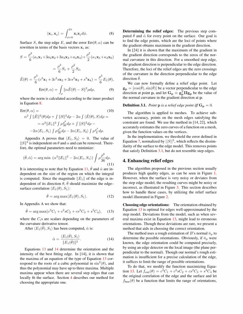
produces high quality edges, as can be seen in Figure 1.However, when the surface is very noisy or deviates fromthe step edge model, the resulting curves might be noisy orincorrect, as illustrated in Figure 3. This section describeshow to handle these cases, by utilizing the relief surfacemodel illustrated in Figure 2.

Choosing edge orientations: The orientation obtained byEquation 13 is optimal for edges well-approximated by thestep model. Deviations from the model, such as when sev-eral maxima exist in Equation 13, might lead to erroneousorientations. Though these deviations are rare, we present amethod that aids in choosing the correct orientation.

The method uses a rough estimation of B’s normal np todetermine the possible orientations. Obviously, if np wereknown, the edge orientation could be computed precisely,by using an edge detector on the local image (the plane per-pendicular to the normal). Though our normal’s rough esti-mation is insufficient for a precise calculation of the edge,it suffices to limit the range of possible orientations.

To do that, we modify the function maximizing Equa-tion 13. Let fcorr(θ) = c3C1 + c2sC2 + cs2C3 + s3C4 bethe original correlation of the edge and the surface and letfbase(θ) be a function that limits the range of orientations,

(a) Relief edges (b) Enhanced relief edgesFigure 3. A late Hellenistic lamp (150-50 BCE): top, full object;bottom, zoom in. Note the closing of the outline of Cupid’s footdue to correcting the edge orientation and the smooth edges result-ing from the smoothing procedure.

using the estimated base normal (defined below). We definethe modified function as:

fmod(θ) = fcorr(θ) · fbase(θ). (15)

If np were known, the edge direction θbase could be cal-culated as the projection of np on the local tangent plane.Then, fbase(θ) = δ(θ − θbase), where δ is the Kroneckerdelta function. Since np is known only approximately, weuse:

fbase(θ) = rw(θ − θbase), (16)

where

rw(x) ={

1 ‖x‖ ≤ w0 ‖x‖ > w.

(17)

Below we describe how to calculate the rough estimationof np and the width w.

To calculate np, the surface (S) normals are smoothed atthe neighborhood of the point. This neighborhood should besufficiently large, so as to reduce the influence of the localfeatures on the estimated normal. Our approach utilizes anadaptive Gaussian filter, similarly to [21]. However, sincethe σ of the smoothing Gaussian in [21] estimates the sizeof the local feature, it is unsuitable for estimating the basesurface. We therefore use a three times larger σ . This en-ables us to average the normals of several features and thusachieve a better approximation.

To calculate width w, we first compute the directionsθbase and θ (Equation 13) for all the vertices. Then, w isset to the standard deviation of the histogram of the error

‖θ − θbase‖. Assuming that most of the values of θ are cor-rect, w is statistically meaningful. When the edge is weak,its gradient estimation is unreliable, and thus it is removed,by setting fbase(θ) ≡ 1. In the implementation, weak edgesare characterized by a small angle between the base normal(∠(np, np) ≤ 11◦). The value 1/(np · np) is proportionalto the magnitude of the local image gradient. This measureis most commonly used to threshold edges.

Since we are utilizing two thresholds – one that measuresthe similarity to the edge model (Section 3.2) and one thatmeasures the edge strength, we can combine them to pro-duce better results using a two-dimensional hysteresis.

Edge smoothing: While the method described above cap-tures the features correctly, scanning noise and edge di-rection estimation errors may cause the edges to becomejagged. In this case, smoothing should be applied. Whilesmoothing could be applied to the edges themselves, thiscorrection would not relate to the geometry of the surface.Therefore, a smoothing scheme which indirectly smoothesthe edges is proposed.

This is done by first smoothing the function Gp, whichis defined at every vertex, yielding Gp. Then, we computethe updated edge directions gp that satisfy:

Gp = gTp IIgp. (18)

When such a direction does not exist (e.g., when Gp is re-quired to have a negative value at a point with two positiveprincipal curvatures), the direction that minimizes the error‖Gp − Gp‖ is chosen. Finally, Gp is recalculated accord-ing to gp.

We observed that good results are achieved when simpleGaussian smoothing is used to smooth Gp. The smoothingparameter can be controlled by the user. In all our experi-ments, the σ of the Gaussian is equal to 0.8 of the medianedge length of the mesh.

5. ResultsThis section shows results of relief edges and compares

them to other major edge families. While relief edges canbe used on any object, as shown in Figure 4, we focus on thechallenging archaeological artifacts, which are noisy andcontain edges which are difficult to detect.

Analysis of archaeological artifacts such as ceramic ves-sels, stone tools, coins, seals and figurines is a major sourceof our knowledge about the past. Traditionally, archaeolog-ical artifacts are drawn by hand and printed in the reports ofarchaeological excavations. These are produced manuallyby artists, in an extremely time-consuming and expensiveprocedure, prone to inaccuracies and biases. The main pur-pose of these drawings is to depict the features of the 3Dobject so that the archaeologist can visualize and compare

The object Relief edgesFigure 4. Elephant. Note that the relief edges are shown togetherwith the surface contours.

artifacts. Thus, all the major features (edges) have to be de-tected. When, in the near future, digitization of the findingsby high resolution scanners will replace the 2D representa-tions, accurate, automatic curve drawing will be needed.

Figures 5–8 show some results. Figures 5–6 demonstratethe importance of choosing the correct orientation of theedges. Since the edges pass on almost flat surfaces, the basenormal can be calculated accurately and aid in estimatingthe edge direction. Figure 6 is a difficult object, due to thehigh level of noise. Locally true edges and noisy surfaceslook similar and therefore demarcating curves fail to differ-entiate between them. Relief edges on the other hand ex-ploit the approximated base for estimating the local imagegradient. In addition, relief edges perform better at placeswhere the curve curvature is not constant.

Figures 7–8 demonstrate models having non-planarbases. In particular, the base surface of Figure 8 is quitecomplex. As can be seen, relief edges outperform the othertypes of edges.

The algorithm was implemented in C++ using thetrimesh2 library by S. Rusinkiewicz. On a 2.66 GHz In-tel Core 2 Duo PC all the steps of the algorithm run in realtime except the estimation of the base normal which cur-rently takes 16 seconds for a surface of 50K vertices and 55seconds for a surface of 140K vertices.

6. ConclusionThis paper has extended the definition of edges from im-

ages to surfaces, for which image edges are a special case.These edges, termed relief curves, use local intrinsic surfaceproperties together with a rough approximation of the basesurface to produce superior results.

The results show that relief edges manage to capturethe 3D features. They have been utilized to draw edgeson scanned objects for artifact illustration in archaeology.In the future we intend to utilize these edges for shape-matching applications, which is an important challenge inarchaeology, as well as in computer vision in general.

Acknowledgements: This research was supported in partby the Israel Science Foundation (ISF) 628/08, the Ollen-dorff foundation, and the Joint Technion University of HaifaResearch Foundation. We thank Dr. A. Gilboa and the Zin-man Institute of Archaeology at the University of Haifa.

References[1] S. Baker, S. Nayar, and H. Murase. Parametric feature detec-

tion. Int. J. of Comp. Vis., 27(1):27–50, 1998.[2] A. Bartoli and P. Sturm. The 3D line motion matrix and

alignment of line reconstructions. Int. J. of Comp. Vis.,57(3):159–178, 2004.

(a) The object (b) Ridges & valleys

(c) Demarcating curves (d) Relief edgesFigure 5. Hellenistic stamped amphora handle from the first century BCE. While the text is hardly legible in the 3D object, relief edgesmake most of the letters visible and improve on the alternatives. The text reads MAPΣΥA APTAMITI◦.

(a) The object (b) Ridges & valleys

(c) Demarcating curves (d) Relief edgesFigure 6. Hellenistic stamped amphora handle from the first century BCE. This is an example of a noisy surface. Only relief edges managedistinguish between the edges and the noise utilizing the approximated base surface.

(a) The object (b) Ridges & valleys

(c) Demarcating curves (d) Relief edgesFigure 7. Hellenistic vase. The figures are well-depicted with long meaningful edges. Note especially the quality of the recovered armswhere the curvature of the edges change considerably .

[3] H. Bay, V. Ferraris, and L. Van Gool. Wide-baseline stereomatching with line segments. IEEE Conf. on Comp. Vis. andPatt. Rec., 1:329 – 336, 2005.

[4] J. Canny. A computational approach to edge detection. IEEETrans. on Patt. Anal. and Mach. Intell., 8(6):679–698, 1986.

[5] F. Cole, A. Golovinskiy, A. Limpaecher, H. S. Barros,A. Finkelstein, T. Funkhouser, and S. Rusinkiewicz. Wheredo people draw lines? ACM Trans. on Graph., 27(3):1–11,2008.

[6] D. DeCarlo, A. Finkelstein, S. Rusinkiewicz, and A. San-tella. Suggestive contours for conveying shape. ACM Trans.on Graph., 22(3):848–855, 2003.

[7] M. P. Do Carmo. Differential geometry of curves and sur-faces. Prentice-Hall, 1976.

[8] D. A. Forsyth and J. Ponce. Computer Vision – A ModernApproach. Prentice-Hall, 2002.

[9] A. Gueziec and N. Ayache. Smoothing and matching of 3Dspace curves. Int. J. of Comp. Vis., 12(1):79–104, 1994.

(a) The object (b) Ridges & valleys (c) Demarcating curves (d) Relief edgesFigure 8. Figurine from the Persian period (4th c. BCE). The relief edges are continuous and smoother than the alternatives. Noisy edgeshave been successfully removed.

[10] E. Hameiri and I. Shimshoni. Estimating the principal curva-tures and the Darboux frame from real 3D range data. IEEESMC B, 33(4):626–637, August 2003.

[11] T. Judd, F. Durand, and E. Adelson. Apparent ridges for linedrawing. ACM Trans. on Graph., 22(3):19:1 – 19:7, 2007.

[12] D. Katsoulas and A. Werber. Edge detection in range imagesof piled box-like objects. ICPR, 2:80–84, 2004.

[13] J. J. Koenderink. Solid Shape. MIT Press, 1990.[14] M. Kolomenkin, I. Shimshoni, and A. Tal. Demarcating

curves for shape illustration. ACM Trans. on Graph., SIG-GRAPH Asia, 27(4), 2008.

[15] T. Langer, A. Belyaev, and H. Seidel. Exact and interpolatoryquadratures for curvature tensor estimation. Comp. AidedGeometric Design, 24(8-9):443–463, 2007.

[16] D. Marr and E. C. Hildreth. Theory of edge detection. Proc.of the Royal Society of London, B(207):187–217, 1980.

[17] P. Meer and B. Georgescu. Edge detection with embeddedconfidence. IEEE PAMI, 23(12):1351–1365, 2001.

[18] K. Mikolajczyk, A. Zisserman, and C. Schmid. Shape recog-nition with edge-based features. British Mach. Vis. Conf.,2:779 – 788, 2003.

[19] O. Monga, R. Deriche, G. Malandain, and J. P. Cocquerez.Recursive filtering and edge tracking: two primary tools for3D edge detection. IVC, 9(4):203–214, 1991.

[20] V. S. Nalwa and T. O. Binford. On detecting edges. IEEETrans. on Patt. Anal. and Mach. Intell., 8(6):699–714, 1986.

[21] Y. Ohtake, A. Belyaev, and H. Seidel. Mesh smoothing byadaptive and anisotropic gaussian filter applied to mesh nor-mals. Vis., Model., and Visual., pages 203–210, 2002.

[22] Y. Ohtake, A. Belyaev, and H. Seidel. Ridge-valley lines onmeshes via implicit surface fitting. ACM Trans. on Graph.,23(3):609–612, 2004.

[23] S. Rusinkiewicz. Estimating curvatures and their derivativeson triangle meshes. In 3D Data Processing, Visualizationand Transmission, pages 486–493, 2004.

[24] V. Torre and T. Poggio. On edge detection. IEEE Trans. onPatt. Anal. and Mach. Intell., 8:147–163, 1986.

[25] X. Xuexiang, H. Ying, T. Feng, and S. Hock-Soon. An ef-fective illustrative visualization framework based on photicextremum lines (PELs). IEEE Trans. on Vis. and Comp.Graph., 13(6):1328–1335, 2007.

[26] S. Zucker and R. Hummel. A three-dimensional edge opera-tor. IEEE PAMI, 3(3):324–331, 1981.

Appendix A: Inner products of polynomialsIn Equation 8, the inner products of the basis functions

need to be computed. When the exponent of sin(φ) orcos(φ) is odd, the inner product is zero. Otherwise, theinner product is defined by the Euler beta function:

B(x, y) = 2∫ π/2

φ=0

(sin(φ))2x−1(cos(φ))2y−1dφ.

Thus, 〈x1,x1〉 = 〈x4,x4〉 = 58π ≡ A,

〈x2,x2〉 = 〈x3,x3〉 = 〈x1,x3〉 = 〈x2,x4〉 =π

8≡ B. (19)

We can now calculate the inner products in Section 3.2:

〈E1, S2〉 = (20)〈c3x1 + 3c2sx2 + 3cs2x3 + s3x4, k1x5 + k2x6〉 = 0,

‖E1‖2 = ‖c3x1 + 3c2sx2 + 3cs2x3 + s3x4‖2 == c6〈x1,x1〉+ 9c4s2〈x2,x2〉+ 9c2s4〈x3,x3〉+s6〈x4,x4〉+ 6c4s2〈x1,x3〉+ 6c2s4〈x2,x4〉

= · · · = ((1− 3c2 + 3c4))A+ 3A(c2 − c4) = A,

〈E1, S1〉 = c3a1〈x1,x1〉+ 9c2sa2〈x2,x2〉++9cs2a3〈x3,x3〉+ s3a4〈x4,x4〉+

+3c3a3〈x1,x3〉+ 3cs2a1〈x1,x3〉+3s3a2〈x2,x4〉+ 3c2sa4〈x2,x4〉 =

= c3(a1A+ 3a3B) + 3c2s(3a2B + a4B)+3cs2(3a3B + a1B) + s3(a4A+ 3a2B) =

= c3C1 + 3c2sC2 + 3cs2C3 + s3C4,

where the Cis are scalars depending on the parameters ofthe curvature derivative tensor (Equation 13).