On Fair Reinsurance Premiums; Capital Injectionsin a Perturbed Risk Model

Zied Ben Salah∗ and Jose Garrido∗∗

Abstract

We consider a risk model where deficits after ruin are covered by a new typeof reinsurance contract that provides capital injections. To allow the insurancecompany’s survival after ruin, the reinsurer injects capital only at ruin timescaused by jumps larger than a chosen retention level. Otherwise capital mustbe raised from the shareholders for small deficits. The problem here is to deter-mine adequate reinsurance premiums. It seems fair to base the net reinsurancepremium on the discounted expected value of any future capital injections. In-spired by the results of Huzak et al. (2004) and Ben Salah (2014) on successiveruin events, we show that an explicit formula for these reinsurance premiumsexists in a setting where aggregate claims are modeled by a subordinator anda Brownian perturbation. Here ruin events are due either to Brownian oscilla-tions or jumps and reinsurance capital injections only apply in the latter case.The results are illustrated explicitly for two specific risk models and in somenumerical examples.

Keywords: reinsurance, capital injections, ruin, successive ruin events, spec-trally negative Levy process, scale function, expected present value, Gerber-Shiu function.

1 Introduction

Reinsurance contracts between a direct insurer and a reinsurer are used to transferpart of the risks assumed by the insurer. The problematic risks are those carrying

∗Corresponding author: Department of Mathematics and Actuarial Sciences. American Uni-versity in Cairo, P.O. Box 74, New Cairo 11835, Egypt. Email: zied.bensalah@aucegypt.edu. Thisauthor gratefully acknowledges the financial support of a B3 Postdoctoral Fellowship from the Fondsde recherche du Quebec - Nature et technologies (FRQNT).

∗∗Department of Mathematics and Statistics. Concordia University, 1455 de Maisonneuve BlvdW, Montreal, Quebec H3G 1M8, Canada. Email: jose.garrido@concordia.ca. This author grate-fully acknowledges the financial support of the Natural Sciences and Engineering Research Council(NSERC) of Canada grant 36860-2017.

1

arX

iv:1

710.

1106

5v4

[q-

fin.

RM

] 1

2 Ju

n 20

18

either the possible occurrence of very large individual losses, the possible accumulationof many losses from non-independent risks, or those from other occurrences thatcould prevent insurers from fulfilling their solvency requirements. So traditionallyreinsurance has been an integral part of insurance risk management strategies (seeCenteno and Simoes, 2009 for a survey of the different types of reinsurance andrecent optimal reinsurance results). However, over time, global financial marketshave developed additional or alternative risk transfer mechanisms, such as swaps,catastrophe bonds or other derivative products, that have helped insurers reducetheir risk mitigation costs.

In this spirit of designing possibly cheaper risk transfer agreements we considerhere a new type of reinsurance contract that would provide capital injections only inextreme, worse scenario cases. It differs from excess–of–loss (XL) agreements, or evencatastrophe XL (Cat XL), in that it is neither a per–risk nor a per–event reinsurancecontract, but rather one based on the insurer’s financial position. Here ruin willserve as a simplifying proxy for the insurer’s financial health. Reinsurance capitalinjections, after ruin, would allow the insurance company to continue operate untilthe next ruin. Again to simplify the analysis we adopt an on-going concern basis andset an infinite horizon for the reinsurance treaty, which can allow repeated ruin events.The reinsurance agreement then calls for a capital injection after these successive ruinevents, keeping the insurer afloat in perpetuity. We call this new type of agreementreinsurance by capital injections (RCI).

Here our jump–diffusion surplus process can generate two types of ruin events,hence different covers are assumed with distinct sources of capital. Surplus fluctua-tions due to jumps are assumed to represent larger claim costs from events unfavorableto the insurer; a ruin caused by such jumps will trigger a capital injection from theextreme-loss reinsurance contract, at ruin time, if the capital injection is larger thana certain threshold (retention limit). By contrast, Brownian oscillations representcomparatively smaller surplus fluctuations; so ruin caused by oscillations should beeasier to cover with capital raised directly from the stockholders. Hence the reinsurerdoes not provide capital injections in cases when (1) ruin is from an oscillation, or(2) when it is from a jump producing a capital injection smaller than the threshold.As explained in the paper, even if stockholders may need cover these 2 types of ruincosts at first, they may ultimately get reimbursed by the reinsurer, at a subsequentruin time due to a jump, if the latter is deep enough to meet the threshold.

Two recent developments in the literature make the analysis of the RCI contractsnow possible, in the sense of getting tractable formulas for net premiums that wouldbe fair to both parties for such agreements. The first one is the development of ac-tuarial and financial models for capital injections (see for instance Einsenberg andSchmidli, 2011, or more recently Avram and Loke, 2018, and the references therein)and the other is the derivation of tractable formulas for the expected present valueof future capital injections in a quite general class of risk models (see Huzak et al.,2004, and Ben Salah, 2014). The application presented here builds on this recent

2

theory to develop fair lump sum net premiums for two types of RCI contracts, bothover an infinite horizon. In practice our net premiums would have to be allocatedto finite policy terms (e.g. a year) and loaded appropriately to define gross (mar-ket) premiums. In this first study we focus on the definition of the RCI contractsand the derivation of the premium formulas so that both, insurance and reinsurancecompanies, can compare the cost of RCI contracts to their alternative risk mitigationstrategies/products. Future work would then need to address the issue of optimizingthe insurance firm value by weighing these premiums in relation to other concurrentcapital injections from shareholders.

To sum up, the paper is organized as follows: the general risk model used here isdefined in Section 2. Then Section 3 covers the preliminary technical results needed toderive the expected present value of future capital injections. Section 4 gives the mainresult, with the derivation of fair premiums for reinsurance based on capital injectionsin the general risk model defined in Section 2. These are illustrated in detail for twoclassical risk processes in Section 5, which gives also numerical illustrations. Thearticle concludes with some general remarks.

2 Risk model

We consider a general insurance surplus model that extends the standard Cramer–Lundberg theory to allow for jumps and diffusion type fluctuations. Here

Rt := x− Yt , t > 0 , (2.1)

where x > 0 is the initial surplus and the risk process Y , a spectrally positive Levyprocess defined on a filtered probability space (Ω,F , (Ft)t>0,P), is given by

Yt := −c t+ St + σBt , t > 0 , (2.2)

where S = (St)t≥0 is a subordinator (i.e. a Levy process of bounded variation andnon–decreasing paths) without a drift (S0 = Y0 = 0) and B is a standard Brownianmotion independent of S. Let ν be the Levy measure of S; that is, ν is a σ–finitemeasure on (0,∞) satisfying

∫(0,∞)

(1∧y)ν(dy) <∞. In this case the Laplace exponent

of S is defined by

ψS(s) =

∫(0,∞)

(es y − 1) ν(dy) ,

where E[esSt ] = et ψS(s).Note that the risk process in (2.1) is similar in spirit to the original perturbed

surplus process introduced in Dufresne and Gerber (1991). The constant x > 0represents the initial surplus, while the process Y models the cash outflow of theprimary insurer and the subordinator S represents aggregate claims. That is why Sneeds to be an increasing process, with the jumps representing the claim amounts

3

paid out. The Brownian motion B accounts for any small fluctuations affecting othercomponents of the risk process dynamics, such as the claim arrivals, premium incomeor investment returns.

Here c t represents aggregate premium inflow over the interval of time [0, t]. Thepremium rate c is assumed to satisfy the net profit condition, more precisely E[S1] < c,which means that ∫

(0,∞)

y ν(dy) < c . (2.3)

Condition (2.3) implies that the process Y has a negative drift, in order to avoid thepossibility that R becomes negative almost surely. This condition is often expressedin terms of a safety loading applied to the net premium. For instance, note that wecan recover the classical Cramer–Lundberg model if σ = 0 and c := (1 + θ)E[S1], forS a compound Poisson process modeling aggregate claims.

We do not use the concept of safety loading in this paper, in order to simplify thenotation, but we stress the fact that this concept is implicitly considered within thedrift of Y when we impose condition (2.3). The classical compound Poisson modelis a special case of this framework where ν(dy) = λK(dy), with λ being the Poissonarrival rate and K a diffuse claim distribution. We refer to Asmussen and Albrecher(2010) for an account on the classical risk model, and to Dufresne and Gerber (1991),Dufresne, Gerber and Shiu (1991), Furrer and Schmidli (1994), Yang and Zhang(2001), Biffis and Morales (2010) and Ben Salah (2014) for the original and differentgeneralizations or studies of the model in (2.2).

Now, one of the main objectives of this paper is to obtain an expression for thereinsurance premium for the risk model in (2.2). First we need to define quantities andnotation associated with the ruin time, as well as the sequence of times of successivedeficits due to a claim of the surplus process (2.2) after ruin. Let τx be the ruin timerepresenting the first passage time of Rt below zero when R0 = x, i.e.

τx := inft > 0 : Yt > x , (2.4)

where we set τx = +∞ if Rt ≥ 0, for all t ≥ 0. We define the first new record time ofthe running supremum

τ := inft > 0 : Yt > Y t− , (2.5)

and the sequence of times corresponding to new records of Y (that is Y t := supYs :t ≥ s) due to a jump of S after the ruin time τx. More precisely, let

τ (1) := τx , (2.6)

and, assuming that τ (n) <∞, then by induction on n ≥ 1:

τ (n+1) := inft > τ (n) : Yt > Y t− , (2.7)

(note that by this definition τ (1) differs from the consecutive new record times (τ (n))n>1;the former includes ruin events caused by jumps and Brownian oscillations, while thelatter include subsequent records only due to jumps).

4

Figure 1: Sample path of Yt = −ct+ St + σBt in (2.2)

Recall from Theorem 4.1 of Huzak et al. (2004) that the sequence (τ (n))n>1 isdiscrete, and, in particular, neither time 0 nor any other time is an accumulationpoint of these τ (n)’s. More precisely, τ > 0 a.s. and τ (n) < τ (n+1) a.s. if τ (n) < ∞.As a consequence, we can order the sequence (τ (n))n≥1 of times when a new supremumis reached by a jump of a subordinator as 0 < τ (1) < τ (2) < · · · a.s.; see Figure 1.

Finally, consider the random number

N := maxn : τ (n) <∞ , (2.8)

which represents the number of new records reached by a claim of the surplus processin (2.2).

Before developing fair premiums for these new reinsurance by capital injectionscontracts that we define here, the next section first presents the theory available forthe spectrally negative Levy risk model defined in (2.2); see [10], [23] and [3] for moredetails.

3 Preliminary results

This section reviews some notions and results needed in the rest of the paper. LetX = (Xt)t>0 be a spectrally negative Levy process defined by

Xt = −Yt = c t− St − σBt .

Since X has no positive jumps, the expectation E[esXt ] exists for all s > 0 and isgiven by E[esXt ] = et ψ(s), where ψ(s) is of the form

ψ(s) = c s+1

2σ2s2 +

∫ ∞0

(e−x s − 1) ν(dx) . (3.1)

5

Here c ∈ R, σ > 0 and ν is the Levy measure associated with the process Y (for athorough account of Levy processes see [6, 23]).

Consider Φ, the right inverse of ψ, defined on [0,∞) by

Φ(q) := sups > 0 : ψ(s) = q . (3.2)

Note that since X is a spectrally negative Levy process X, we have that Φ(q) > 0 forq > 0 (see [23]).

It is well–known that, for every q > 0, there exists a function W (q) : R −→ [0,∞)such that W (q)(y) = 0, for all y < 0 satisfying∫ ∞

0

e−λyW (q)(y) dy =1

ψ(λ)− q, λ > Φ(q) . (3.3)

These are the so–called q-scale functions W (q), q > 0 of the process X (see [23]),a key notion in the analysis of passage times for spectrally negative Levy processes.Note that for q = 0, equation (3.3) defines the so–called scale function and we simplywrite W := W (0).

The following theorem plays a key role here (we refer to [4] for a thorough dis-cussion and the proof). It gives an expression for a general form of the expecteddiscounted penalty function (EDPF), EP(F, q, x), defined in [4] as

EP(F, q, x) = E[ N∑n=1

e−q τ(n)

Fn(Yτ (n−1) , Yτ (n)) : τx <∞], (3.4)

where F = (Fn)n≥0 is a sequence of given non–negative measurable functions fromR+ × R+ to R, and where x, q ≥ 0 are also given. This generalizes the prior resultson the EDPF in [20] and [16].

Let H ∗G(·) denote the convolution of H(·) with G(·) defined by∫A

f(u)H ∗G(du) =

∫y+v∈A

f(y + v)H(dy)H(dv) ,

for any Borel set A of R×R and nonnegative, bounded Borel function f . As usual f ∗n,for n ≥ 1, denotes the n–fold convolution of f with itself and f ∗0 is the distributionfunction corresponding to the Dirac measure at zero. For more details about thisresult, we refer to [4].

Theorem 3.1 Consider the risk model in (2.2). For x, q ≥ 0, the extended EDPF isgiven by

EP(F, q, x) = φ(w, q, x) +∞∑n=0

∫(x,∞)

∫(0,∞)

eΦ(q) (u+v)Fn+2(v, u+ v)

×H ∗G(du)H∗n ∗G∗n ∗ Tx(dv) , (3.5)

6

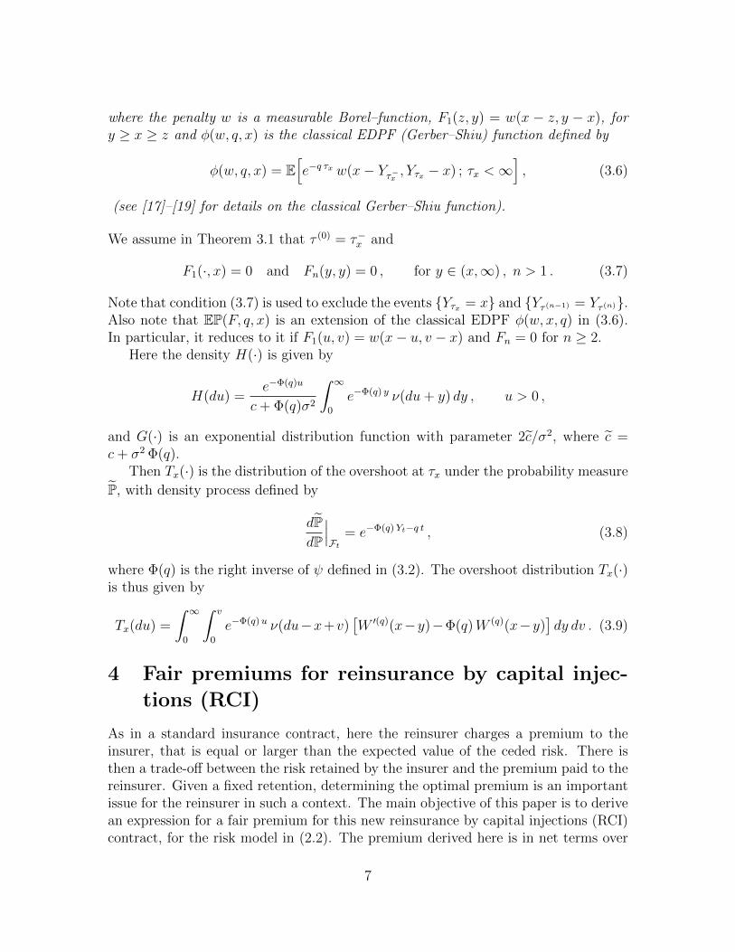
where the penalty w is a measurable Borel–function, F1(z, y) = w(x − z, y − x), fory ≥ x ≥ z and φ(w, q, x) is the classical EDPF (Gerber–Shiu) function defined by

φ(w, q, x) = E[e−q τx w(x− Yτ−x , Yτx − x) ; τx <∞

], (3.6)

(see [17]–[19] for details on the classical Gerber–Shiu function).

We assume in Theorem 3.1 that τ (0) = τ−x and

F1(·, x) = 0 and Fn(y, y) = 0 , for y ∈ (x,∞) , n > 1 . (3.7)

Note that condition (3.7) is used to exclude the events Yτx = x and Yτ (n−1) = Yτ (n).Also note that EP(F, q, x) is an extension of the classical EDPF φ(w, x, q) in (3.6).In particular, it reduces to it if F1(u, v) = w(x− u, v − x) and Fn = 0 for n ≥ 2.

Here the density H(·) is given by

H(du) =e−Φ(q)u

c+ Φ(q)σ2

∫ ∞0

e−Φ(q) y ν(du+ y) dy , u > 0 ,

and G(·) is an exponential distribution function with parameter 2c/σ2, where c =c+ σ2 Φ(q).

Then Tx(·) is the distribution of the overshoot at τx under the probability measure

P, with density process defined by

dPdP

∣∣∣Ft

= e−Φ(q)Yt−q t , (3.8)

where Φ(q) is the right inverse of ψ defined in (3.2). The overshoot distribution Tx(·)is thus given by

Tx(du) =

∫ ∞0

∫ v

0

e−Φ(q)u ν(du−x+v)[W ′(q)(x−y)−Φ(q)W (q)(x−y)

]dy dv . (3.9)

4 Fair premiums for reinsurance by capital injec-

tions (RCI)

As in a standard insurance contract, here the reinsurer charges a premium to theinsurer, that is equal or larger than the expected value of the ceded risk. There isthen a trade-off between the risk retained by the insurer and the premium paid to thereinsurer. Given a fixed retention, determining the optimal premium is an importantissue for the reinsurer in such a context. The main objective of this paper is to derivean expression for a fair premium for this new reinsurance by capital injections (RCI)contract, for the risk model in (2.2). The premium derived here is in net terms over

7

an infinite contract term. For annual or other short–term reinsurance contracts, ourpremium would have to be allocated to each annual/other interval. This is howeverbeyond the scope of this first study, as is the optimization of the choice of reinsuranceretention/premium for these RCI treaties.

We consider two types of RCI contracts, proportional RCI and extreme–loss RCI,which can be combined to design contracts that would be more appropriate in practice.For proportional RCI, the “proportion” of risk ceded to the reinsurer for a claim ofsize C is aC , where a < 1. While in the extreme–loss case the ceded amount of risk tothe reinsurer is C IC≥m , where m ≥ 0. That is, the ceded amount of risk is the totaldeficit C if C exceeds a certain level of retention m ≥ 0, and 0 otherwise. The reasonto set a < 1 in the proportional RCI contract is to avoid moral hazard, a problemnot present with the proposed extreme–loss RCI design. Note, however that from apurely mathematical point of view, the proportional RCI premium formulas beloware also valid for a ≥ 1, so that the capital injections provide the insurer sufficientfunds to recover from ruin and restart from a solvent position, without a need to raiseadditional capital from stockholders.

Based on the above preliminary results, an explicit form for fair RCI net premiums,defined as the discounted value of future capital injections, is:

Π(q, x, r(·)) = E[ N∑n=0

e−q τ(n+1)

r(Cn)], (4.1)

where r(Cn) is given either by r(Cn) = aCn (proportional case) or r(Cn) = Cn ICn≥m(extreme–loss). Note that here Cn denotes the size of the n-th reinsurance claim afterruin (the n-th capital injection), that is

Cn = Rτ (n) −Rτ (n+1)

= Yτ (n+1) − Yτ (n) , for n ≥ 1 , (4.2)

and C0 = Yτ (1) − x, for n = 0, where (τ (n))n≥1 is the sequence of insurer’s claim timescorresponding to new records of Y , defined in Section 2, in Equations (2.6) and (2.7).

Also note that the extreme–loss capital injections occur at times τ (n), of newrecords set by jumps. No capital injections are received if the surplus creeps belowthe threshold barrier only due to Brownian oscillations, without jumps. However,the cost of the Brownian oscillations between 2 record jumps is always included inthe capital injection at the next record jump. The interpretation here is that in ourmodel Brownian oscillations represent (smaller) capital requirements that are lesslikely to amount to a deficit creeping over the solvency threshold m, and hence suchcapital can be provided more easily by stockholders. By contrast, the subordinatorjumps here represent larger (less predictable) losses that should cross the thresholdmore frequently and/or more deeply and for which the insurer needs the reinsurancecapital injections. Clearly such a reinsurance scheme is best suited for companies with

8

observed surplus experience where deficits caused by jumps dominate those causedby oscillations.

The following theorem gives expressions for the RCI premiums in both, the pro-portional and extreme–loss cases, in terms of q–scale functions, where q is the presentvalue discounting rate and the Levy measure. This is the main contribution and it isbased on the result of Theorem 3.1.

Theorem 4.1 Consider the risk model introduced in (2.2):1. The extreme–loss RCI reinsurance premium for r(Cn) = Cn ICn≥m in (4.1) isgiven by

Π1(q, x,m) = ϕ(q, x,m) + δ(q, σ,m)κ(q, x) , (4.3)

where

δ(q, σ,m) =c[2q + Φ(q)(ρ+m− 1)(2c+ Φ(q)σ2)

]qΦ(q)(2c+ Φ(q)σ2)

e−2 c+φ(q)σ2

σ2 m

+2c+ Φ(q)σ2

qσ2

∫ m

0

e−2c+Φ(q)σ2

σ2 v[ ∫ ∞

0

[1 + (mΦ(q)− 1)e−Φ(q)u]

×ν(u+m− v, ∞) du]dv .

2. The proportional RCI reinsurance premium for r(Cn) = aCn in (4.1) is given by

Π2(q, x, a) = aϕ(q, x, 0) + a δ(q, σ, 0)κ(q, x) . (4.4)

The functions κ(q, x) and ϕ(q, x,m) are given explicitly in terms of the q–scale func-tion and the Levy measure as:

ϕ(q, x,m) = f ∗ hm(x) (4.5)

andκ(q, x) = f ∗ t(x) , (4.6)

wheref(x) = W ′(q)(x)− Φ(q)W (q)(x) ,

hm(x) = eΦ(q)x

∫ ∞x

e−Φ(q) v

∫(v,∞)

(u− v) ν(du+m) dv (4.7)

and

t(x) = eΦ(q)x

∫ ∞x

e−Φ(q) v ν(v,∞) dv . (4.8)

Proof: 1. Consider the sequence of functions F1(·, y) = (y − x) Iy−x≥m for y > xand Fn(v, u) = (u− v) Iu−v≥m, for u ≥ v > x and n ≥ 2, then the extended EDPF

9

associated with F and q, EP(F, q, x), in Theorem 3.1, is equal to the extreme–loss RCIreinsurance premium Π1(q, x,m). In fact, using Theorem 3.1, we can derive (4.3):

Π1(q, x,m) = E[e−qτx (Yτx − x) IYτx−x≥m; τx <∞

]+∞∑n=0

∫(x,∞)

∫(0,∞)

eΦ(q)(u+v) u Iu≥m (H ∗G)(du)(H∗n ∗G∗n ∗ Tx)(dv)

= ϕ(q, x,m) +

∫(0,∞)

eΦ(q)u u Iu≥mH ∗G(du)

∞∑n=0

∫(x,∞)

eΦ(q)vH∗n ∗G∗n ∗ Tx(dv)

= ϕ(q, x,m) + κ(q, x)

∫(m,∞)

eΦ(q)u uH ∗G(du)︸ ︷︷ ︸Im

∞∑n=0

[ ∫(0,∞)

eΦ(q)vH ∗G(dv)︸ ︷︷ ︸I

]n, (4.9)

whereϕ(q, x,m) = E

[e−q τx (Yτx − x) IYτx−x ≥m ; τx <∞

]and

κ(q, x) =

∫(x,∞)

eΦ(q) v Tx(dv) = E[e−q τx ; τx <∞] , (4.10)

since Tx(dv) = P(Yτx ∈ dv, τx <∞), for v > x.

Now the term I in (4.9) is equal to

I =

∫ ∞0

eΦ(q)uH ∗G(du) =

∫ ∞0

eΦ(q)uH(du)

∫ ∞0

eΦ(q)uG(du) . (4.11)

The first integral in the above equation is given by∫(0,∞)

eΦ(q)uH(du) =1

c+ Φ(q)σ2

∫ ∞0

e−Φ(q) y ν(y, ∞) dy

=2cΦ(q) + σ2Φ(q)2 − 2q

2Φ(q)[c+ Φ(q)σ2

] , (4.12)

where the last equality uses the identity ψ(Φ(q)) = q and integration by parts.The second integral in (4.11) is∫

(0,∞)

eΦ(q)uG(du) =2[c+ φ(q)σ2]

2c+ φ(q)σ2. (4.13)

10

By substituting (4.12) and (4.13) in (4.11), we conclude that∫(0,∞)

eΦ(q)uH ∗G(du) = 1− 2q

Φ(q)[2c+ σ2Φ(q)

] ∈ (0, 1) .

Finally the term Im in (4.9) is equal to

Im =

∫u+v>m

eΦ(q)(u+v)(u+ v)H(du)G(dv)

=

∫u>0

∫v>m

eΦ(q)(u+v)(u+ v) H(du)G(dv)︸ ︷︷ ︸I1m

+

∫u>m−v

∫0<v<m

eΦ(q) (u+v) (u+ v)H(du)G(dv)︸ ︷︷ ︸I2m

= I1m + I2

m , (4.14)

where

I1m =

∫(0,∞)

eΦ(q)u[ ∫

(m,∞)

(u+ v) eΦ(q)v G(dv)]H(du)

= e−[2 c+φ(q)σ2

σ2 ]m

∫(0,∞)

eΦ(q)u[u

∫ ∞0

2c

σ2e−[ 2c

σ2−Φ(q)]v dv

+

∫ ∞0

2c

σ2(v +m) e−[ 2c

σ2−Φ(q)]v dv]H(du)

= e−[2 c+φ(q)σ2

σ2 ]m

∫(0,∞)

eΦ(q)u[2(c+ Φ(q)σ2)

2c+ Φ(q)σ2

(u+m+

σ2

2c+ Φ(q)σ2

)]H(du)

= e−[2 c+φ(q)σ2

σ2 ]m 2

2c+ Φ(q)σ2

[( σ2

2c+ Φ(q)σ2+m

) ∫(0,∞)

e−Φ(q)y ν(y,∞) dy

+

∫ ∞0

∫(0,∞)

u e−Φ(q)y ν(du+ y) dy]

= e−[ 2cσ2 +Φ(q)]m 2

2c+ Φ(q)σ2

[( σ2

2c+ Φ(q)σ2+m

) ∫(0,∞)

e−Φ(q)y ν(y,∞) dy

+1

Φ(q)

[ ∫ ∞0

ν(y,∞) dy −∫ ∞

0

e−Φ(q)yν(y,∞) dy]]

= e−[2 c+φ(q)σ2

σ2 ]m 2

2c+ Φ(q)σ2

[( σ2

2c+ Φ(q)σ2− 1

Φ(q)+m

)×∫

(0,∞)

e−Φ(q)y ν(y,∞)dy +1

Φ(q)E[S1]

]= e−[

2 c+φ(q)σ2

σ2 ]m 2 c[2q + Φ(q)(ρ+m− 1)(2c+ Φ(q)σ2)

]Φ(q)2 [2c+ Φ(q)σ2]2

(4.15)

11

and where in the last equality we used (4.12).The second term I2

m in (4.14) is given by

I2m =

∫0<v<m

∫u>m−v

(u+ v) eΦ(q)ueΦ(q)vG(dv)H(du)

=

∫0<v<m

G(dv)

∫u>0

(u+m) eΦ(q)(u+m) H(du+m− v)

=2

σ2

∫0<v<m

e−[2c+Φ(q)σ2

σ2 ]v dv

∫u>0

∫ ∞0

(u+m) e−Φ(q)y ν(du+m− v + y) dy

=2

σ2

∫0<v<m

e−[2c+Φ(q)σ2

σ2 ]vdv

∫ ∞0

e−Φ(q)y

∫u>0

(u+m) ν(du+m− v + y) dy

=2

σ2

∫0<v<m

e−[2c+Φ(q)σ2

σ2 ]v

∫ ∞0

e−Φ(q)y[ ∫ ∞

y

ν(u+m− v, ∞) du

+ν(y +m− v, ∞)]dy dv

=2

σ2

∫0<v<m

e−[2c+Φ(q)σ2

σ2 ]v 1

Φ(q)

[ ∫ ∞0

ν(u+m− v, ∞) du (4.16)

−∫ ∞

0

e−Φ(q)yν(y +m− v, ∞) dy]dv

=2

Φ(q)σ2

∫ m

0

e−[2c+Φ(q)σ2

σ2 ]v[ ∫ ∞

0

[1 + (mΦ(q)− 1)e−Φ(q)u]

× ν(u+m− v, ∞) du]dv . (4.17)

Finally, using the expressions above for Im in (4.14) and I in (4.11), then (4.9) isequal to

Π1(q, x,m) = ϕ(q, x,m) + (I1m + I2

m)∞∑n=0

[I]n︸ ︷︷ ︸δ(q,σ,m)

κ(x, q)

= ϕ(q, x,m) + δ(q, σ,m)κ(x, q) , (4.18)

where

δ(q, σ,m) =c[2q + Φ(q) (ρ+m− 1) (2c+ Φ(q)σ2)

]qΦ(q) [2c+ Φ(q)σ2]

e−[2 c+φ(q)σ2

σ2 ]m

+[2c+ Φ(q)σ2]

qσ2

∫ m

0

e−[2c+Φ(q)σ2

σ2 ]v[ ∫ ∞

0

[1 + (mΦ(q)− 1) e−Φ(q)u]

× ν(u+m− v, ∞) du]dv .

Now, to complete the proof of the theorem, we need only to identify the two functionsϕ(q, x,m) and κ(x, q). Recall Lemma 4.1 in [4] that gives an explicit form for the

12

classical EDPF, φ(w, q, x), defined in (3.6). With it we can derive explicit expressionsfor the above functions ϕ(q, x,m) and κ(x, q):

κ(q, x) = E[e−q τx ; τx <∞]

= f ∗ t(x) , (4.19)

wheref(x) = W ′(q)(x)− Φ(q)W (q)(x) (4.20)

and

t(x) = eΦ(q)x

∫ ∞x

e−Φ(q) v ν(v,∞)dv , (4.21)

while

ϕ(q, x,m) = E[e−q τx (Yτx − x) IYτx−x ≥m ; τx <∞

]= E

[eΦ(q)Yτx (Yτx − x) IYτx−x ≥m ; τx <∞

]=

∫ ∞0

eΦ(q)u (u+m)Tx(du+ x+m) = f ∗ hm(x) , (4.22)

where E is the expectation under P, Tx(·) is the overshoot distribution defined in (3.9)and

hm(x) = eΦ(q)x

∫ ∞x

e−Φ(q) v

∫(0,∞)

(u+m) ν(du+ v +m) dv . (4.23)

Then the first part of the theorem follows.

2. Following the same order of ideas above, the second part of Theorem 4.1 can be eas-ily shown. In fact, the expression of the extended EDPF in (3.5) reduces the propor-tional RCI premium, since here we take F1(v, u) = a (u−x) and Fn(v, u) = a (u− v) ,

13

for u ≥ 0, v ∈ R and n ≥ 2. Hence

Π2(q, x, a) = E[e−q τx a (Yτx − x) ; τx <∞

]+

∞∑n=0

∫ ∞x

∫ ∞0

eΦ(q) (u+v) a uH ∗G(du)H∗n ∗G∗n ∗ Tx(dv)

= aϕ(q, x, 0) + a κ(q, x)

∫ ∞0

eΦ(q) (u+v) uH ∗G(du)︸ ︷︷ ︸I0

×∞∑n=0

[ ∫ ∞0

eΦ(q) vH ∗G(dv)︸ ︷︷ ︸I

]n

= aΠ1(q, x, 0) = aϕ(q, x, 0) + a I0

∞∑n=0

[II]n κ(q, x)

= aϕ(q, x, 0) + ac[2q + φ(q)(ρ− 1)[2c+ φ(q)σ2]

]qφ(q)[2c+ φ(q)σ2]︸ ︷︷ ︸

δ(q,σ,0)

κ(q, x)

= aϕ(q, x, 0) + a δ(q, σ, 0)κ(q, x) . (4.24)

The following section illustrates the results above for two particular cases, includ-ing the Cramer–Lundberg risk model, without a Brownian component.

5 Examples: two classical risk models

We study in this section particular examples of risk process Y satisfying the generalsetting described in Section 2 for which the q–scale function has a tractable form.These provide some interesting examples of insurance models with relatively simpleexpressions for the reinsurance by capital injections (RCI) premiums.

In fact, a tractable form for the q–scale function is here inherited by the functionsϕ(q, x,m) and κ(q, x), defined in (4.5) and (4.10) respectively. These functions arekey ingredients in the general expressions of Theorem 4.1. In what follows we analyzein more detail some models for which we can have an explicit understanding of thereinsurance premium problem:

• the classical Cramer–Lundberg model with exponential claims,

• the spectrally negative stable risk process.

14

5.1 Classical Cramer–Lundberg model with exponential claims

The so–called classical or Cramer–Lundberg model was introduced in [24]. The sur-plus process is a compound Poisson process starting at x > 0, i.e.,

Rt = x+ ct−Nt∑i=1

Zi , (5.1)

where the number of claims is assumed to follow a Poisson process (Nt)t>0 withintensity λ, independent of the positive and iid random variables (Zn)n>1 representingclaim sizes. The loaded premium c is of the form c = (1 + θ)λE[Z1] for some safetyloading factor θ > 0. The form of the q–scale function in this model is relativelysimple when claim sizes are exponentially distributed with mean 1/µ. In this case,the Levy measure takes the simple form ν(dx) = λµ e−µxdx. In turn, the Laplaceexponent in (3.1) becomes

ψ(s) = c s− λ s

µ+ s, s > 0 . (5.2)

So, the premium rate is c = λ (1 + θ)/µ where θ > 0 is a positive security loading.This model has been for long a textbook example for which the distribution of

ruin–related quantities can be explicitly computed. Here, we study in detail theRCI reinsurance premium for this particular example. Moreover, we derive explicitexpressions for the RCI premiums from Theorem 4.1.

The expression for the q–scale function in this case is known (see [22]) and is givenby

W (q)(x) =µ+ Φ(q)

ηqeΦ(q)x − µ+ Θ(q)

ηqeΘ(q)x , (5.3)

where Φ(q) and Θ(q) are the solutions of ψ(s) = q, i.e. Φ(q) = 12c

(q + λ − c µ + ηq)

and Θ(q) = 12c

(q + λ− c µ− ηq), with ηq =√

(q + λ− c µ)2 + 4q µ c. For details see[22].

In this case, the expressions for κ(q, x) and ϕ(q, x,m) in (4.10) and (4.5) are givenby

ϕ(q, x,m) = f ∗ hm(x) (5.4)

andκ(q, x) = f ∗ t(x) , (5.5)

where

f(x) =[µ+ Θ(q)] [Φ(q)−Θ(q)]

ηqeΘ(q)x

=[µ+ Θ(q)

c

]eΘ(q)x , (5.6)

15

t(x) =λ

(Φ(q) + µ)e−µx (5.7)

and

hm(x) =λ [mµ+ 1]

µ [Φ(q) + µ]e−µ (x+m) . (5.8)

Hence the expressions of κ(q, x) and ϕ(q, x,m) reduce to

ϕ(q, x,m) =λ e−µm [mµ+ 1]

µ c [µ+ Φ(q)][eΘ(q)x − e−µx] (5.9)

and

κ(q, x) =λ

c [µ+ Φ(q)][eΘ(q)x − e−µx] . (5.10)

Recall that in this model, the Brownian component vanishes and then the distributionG(·) reduces to a Dirac measure at 0. Hence, the expression for Im in (4.14) is equalto ∫

u>m

eΦ(q)u uH(du) =λ (mµ+ 1)

c µ [Φ(q) + µ]e−µm , (5.11)

and II reduces to ∫u>0

eΦ(q)uH(du) = 1− q

Φ(q) c.

Using Theorem 4.1, we provide explicit expressions for the RCI reinsurance pre-miums. In fact, in the case of the classical model σ = 0 and hence the extreme–lossRCI premium in (4.3) reduces to

Π1(q, x,m) = ϕ(q, x,m) +λΦ(q) (mµ+ 1) e−µm

µ q [µ+ Φ(q)]κ(q, x)

=λe−µm (mµ+ 1)

µ c [µ+ Φ(q)]

[eΘ(q)x − e−µx

] (1 +

λΦ(q)

q[µ+ Φ(q)]

)=

λΦ(q)e−µm (mµ+ 1)

µ q [µ+ Φ(q)]

[eΘ(q)x − e−µx

]. (5.12)

Similarly, the proportional RCI premium in (4.4) reduces to

Π2(q, x, a) = aΠ1(q, x, 0)

=λ aΦ(q)

µ q [µ+ Φ(q)]

[eΘ(q)x − e−µx

], (5.13)

where, recall, q is the discount factor, x the initial surplus and a < 1 the factor appliedto the risks ceded when a reinsurance capital injection is needed.

16

5.2 Spectrally negative stable process

In this subsection, we study the case when the surplus process is driven by a spectrallynegative stable process with stability parameter α ∈ (1, 2). This model was studiedin the insurance context in [14]. We calculate here the RCI reinsurance premium andgive explicit expressions for both, proportional and extreme–loss RCI contracts.

Let (Xt)t≥0 be a spectrally negative stable process with stability parameter α ∈(1, 2) and Laplace exponent ψ(s) = (s+ c)α− cα, for c, s > 0. Here the Levy measurein (3.1) is given by ν(dx) = e−c x

x1+α Γ(−α)dx, for x > 0 and Γ(u) is the gamma function.

It can be seen (for example [5, 7]) that

W (q)(x) = e−c x xα−1Eα,α[(q + cα)xα

], (5.14)

for x, q > 0, where Eα,β(z) =∑

k>0zk

Γ(β+αk)is the two–parameter Mittag–Leffler

function. It is clear that here Φ(q) = (q + cα)1α − c.

The expressions for κ(q, x) and ϕ(q, x,m) then reduce to

ϕ(q, x,m) =e−cm

x1+α Γ(−α)

∫ ∞0

∫ ∞0

(u+m) e[(q+cα)1/α−c] (x−v) e−c (u+v)

(u+ v +m)α

×[e−(q+cα)1/α x xα−1Eα,α

[(q + cα)xα

]]du dv

− e−cm

x1+α Γ(−α)

∫ ∞0

∫ x

0

(u+m) e[(q+cα)1/α−c] (x−v) e−c (u+v)

(u+ v +m)α

×[e−(q+cα)1/α (x−v) (x− v)α−1Eα,α

[(q + cα) (x− v)α

]]du dv , (5.15)

and

κ(q, x) =1

x1+α Γ(−α)

∫ ∞0

∫ ∞0

e[(q+cα)1/α−c] (x−v) e−c (u+v)

(u+ v)α

×[e−(q+cα)1/α x xα−1Eα,α

[(q + cα)xα

]]du dv

− 1

x1+α Γ(−α)

∫ ∞0

∫ x

0

e[(q+cα)1/α−c] (x−v) e−c (u+v)

(u+ v)α

×[e−(q+cα)1/α (x−v) (x− v)α−1Eα,α

[(q + cα) (x− v)α

]]du dv . (5.16)

As in the previous model, the distribution G(·) reduces to a Dirac measure at 0.Hence, the expression for Im in (4.14) here is equal to

Im =

∫u>m

eΦ(q)u uH(du) =e−cm

Γ(−α)

∫ ∞0

∫ ∞0

e−c (u+m) e−(q+cα)1/α y

(u+ y +m)1+αdy du ,

and I in (4.11) reduces to here

I =

∫u>0

eΦ(q)uH(du) = 1− q

Φ(q) c= 1− q

c [(q + cα)1/α − c].

17

Using Theorem 4.1, we can give explicit expressions for the RCI reinsurance premiums.The extreme–loss RCI premium in (4.3) reduces to

Π1(q, x,m) = ϕ(q, x,m) + κ(q, x)[c e−cm[(q + cα)1/α − c]

q Γ(−α)

]×[ ∫ ∞

0

∫ ∞0

(u+m) e−c u e−(q+cα)1/α y

(u+ y +m)1+αdy du

]. (5.17)

Similarly, the proportional RCI premium in (4.4) reduces to

Π2(q, x, a) = aΠ1(q, x, 0)

= aϕ(q, x, 0) +[a c[(q + cα)1/α − c]

q Γ(−α)

]×[ ∫ ∞

0

∫ ∞0

u e−c u e−(q+cα)1/α) y

(u+ y)1+αdy du

]κ(q, x) . (5.18)

where ϕ(q, x,m) and κ(q, x) are given respectively by (5.15) and (5.16), which aresufficiently explicit to evaluate numerically with such programs as Maple, Matlab orMathematica.

5.3 Numerical examples

To show the tractability of the RCI premium formulas derived above, in the twoprevious sections, we include here a few numerical illustrations. The premium valueswere obtained in Python; the code is available to interested readers upon request.

For these numerical illustrations the Poisson parameter of the classical risk modelin (5.1) was set to λ = 1 as well as the mean exponential claim size µ = 1. Figures 2–3show the effect on the extreme–loss RCI premiums Π1(q, x,m), in (5.12), of varyingthe remaining decision variables, such as the RCI retention level m, the discountfactor q, the premium safety loading θ and the initial surplus x.First, Figure 2(a) plots curves of Π1(q, x,m) versus varying values of the RCI retentionlevel m, for different discount factors q, with an initial surplus of x = 2.5 and safetyloading factor of θ = 0.25. Then Figure 2(b) studies the effect of the loading factorθ on Π1(q, x,m) for an initial surplus of x = 4.5 and discount factor q = 0.05, againversus varying values of the RCI retention level m. Similarly, Figure 2(c) shows curvesagainst the retention level m for different initial surplus values x, with a loading ofθ = 0.5 and discount factor q = 0.05.

Figure 3(a) gives RCI premiums as a function of the security loading θ, for differentvalues of the retention levels m, with initial surplus x = 4.0 c and discount factorq = 0.05, while Figure 3(b) gives RCI premium curves, also as a function of θ, fordifferent q values and retention level m = 1. Finally Figure 3(c) gives RCI premiumcurves, as a function of θ, for different initial surplus values x.From the curves of Π1(q, x,m) in Figures 2 and 3 we see that:

18

(a) Π1(q, x,m) curves by discount factor q (b) Π1(q, x,m) curves by loading θ

(c) Π1(q, x,m) curves by initial surplus x

Figure 2: Extreme–loss RCI premiums Π1(q, x,m) versus retention level m

• Doubling the safety loading θ in Figure 2(a) or the initial surplus x in Figure2(b) has a greater effect on RCI premiums than increasing the discounting rateq by a factor of 10 in Figure 2(c).

• The same is seen from the curves of Π1(q, x,m) versus the safety loading θ inFigure 3, the impact of the discounting factor q is smaller than that of varyingthe retention level m or that of the initial surplus x.

• However, an analysis without discounting (q = 0) is not possible for small valuesof the RCI retention level m or safety loading θ; the present value increaseswithout bound with the more frequent ruin events.

19

(a) Π1(q, x,m) curves by retention level m (b) Π1(q, x,m) curves by discounting factor q

(c) Π1(q, x,m) curves by initial surplus x

Figure 3: Extreme–loss RCI premiums Π1(q, x,m) versus loading factor θ

Conclusion

We consider here a new type of reinsurance contract (RCI) that provides capital injec-tions only in extreme, worse scenario cases, based on the insurer’s financial position.Ruin serves as a simplifying proxy for the insurer’s financial health. Reinsurance cap-ital injections made after each ruin event allow the insurance company to continueoperate indefinitely, as in an on-going concern basis over an infinite horizon.

Borrowing from recent developments in the actuarial and financial literature onmodels for capital injections (e.g. Einsenberg and Schmidli, 2011) and the formulasfor the expected present value of future capital injections in a quite general class ofrisk models (Ben Salah, 2014) we develop fair lump sum net premiums for two typesof RCI contracts. In this first study we show that tractable formulas can be derivedfor RCI premiums so that both, insurance and reinsurance companies, can comparethe cost of RCI contracts to their alternative risk mitigation strategies/products. We

20

also show that an analysis with discounting leads to unstable numerical calculationswhen ruin events become more frequent, as for example when small RCI retentionlevels or small safety loadings θ are chosen.

Further research should tackle the practical problems of premium allocation tofinite (e.g. one year) contract terms, defining reserves and designing other types ofRCI contracts, apart from the proportional and extreme–loss agreements studied here.The problem of optimal control of these new RCI contracts is also a natural questionto be studied if these treaties turn out to be useful and viable; in particular theoptimal stochastic control strategies to choose the appropriate reinsurance retentionlevels and the capital raised from stockholders to temporarily cover the Brownianoscillations. The latter should be easier to control as these will occur continuouslyaround the ruin barrier.

Acknowledgments

The authors are sincerely grateful to Prof. Christian Hipp for his suggestions on anearlier version of this paper and to the two anonymous reviewers for their constructivecomments. This research was partially completed during a sabbatical visit of thesecond author to the University Carlos III of Madrid, in Spain.

References

[1] Asmussen, S. and Albrecher, H. (2010). Ruin Probabilities. World Scientific Publishing,London.

[2] Avram, F. and Loke, S.-H. (2018). On central branch/reinsurance risk networks: exactresults and heuristics. Risks. 6(35), http://dx.doi.org/10.3390/risks6020035.

[3] Avram, F., Palmowski, Z. and Pistorius, M.R. (2007). On the optimal dividend problemfor a spectrally negative Levy process. The Annals of Applied Probability. 17(1), 156-180.

[4] Ben Salah, Z. (2014). On a generalization of the expected discounted penalty function toinclude deficits at and beyond ruin. European Actuarial Journal. 4(4), 219-246.

[5] Ben Salah, Z., Guerin, H., Morales, M. and Omidi Firouzi, H. (2015). On the depletionproblem for an insurance risk process: new non-ruin quantities in collective risk theory.European Actuarial Journal. 5(2), 381-425.

[6] Bertoin, J. (1998). Levy Processes. Cambridge University Press.

[7] Biffis, E. and Kyprianou, A.E. (2010). A note on scale function and the time value ofruin. Insurance: Mathematics and Economics. 46, 85-91.

[8] Biffis, E. and Morales, M. (2010). On a generalization of the Gerber-Shiu function topath-dependent penalties. Insurance: Mathematics and Economics. 46, 92-97.

21

[9] Centeno, M.L. and Simoes, O. (2009). Optimal reinsurance. Revista de la Real Academiade Ciencias, Serie - A, Matematicas. 103(2), 387-405.

[10] Doney, R. and Kyprianou, A.E. (2006). Overshoots and undershoots of Levy processes.The Annals of Applied Probability. 16(1), 91-106.

[11] Dufresne, F. and Gerber, H. (1991). Risk theory for compound Poisson process that isperturbed by diffusion. Insurance: Mathematics and Economics. 10, 51-59.

[12] Dufresne, F., Gerber, H. and Shiu, E.W. (1991). Risk theory with gamma process.ASTIN Bulletin. 21, 177-192.

[13] Einsenberg, J. and Schmidli, H. (2011). Minimising expected discounted capital injec-tions by reinsurance in a classical risk model. Scandinavian Actuarial Journal. 3, 155-176.

[14] Furrer, H.J. (1998). Risk processes perturbed by α-stable Levy motion. ScandinavianActuarial Journal. 1, 59-74.

[15] Furrer, H.J. and Schmidli, H. (1994). Exponential inequalities for ruin probabilities ofrisk processes perturbed by diffusion. Insurance: Mathematics and Economics. 15, 23-36.

[16] Garrido, J. and Morales, M. (2006). On the expected penalty function for Levy riskprocess. North American Actuarial Journal. 10(4), 196-218.

[17] Gerber, H. and Shiu, E. (1997). The joint distribution of the time of ruin, the surplusimmediately before ruin, and the deficit at ruin. Insurance: Mathematics and Economics.21, 129-137.

[18] Gerber, H. and Shiu, E. (1998a). On the time value of ruin. North American ActuarialJournal. 2(1), 48-78.

[19] Gerber, H. and Shiu, E. (1998b). Pricing perpetual options for jump processes. NorthAmerican Actuarial Journal. 2(3), 101-112.

[20] Gerber, H. and Landry, B. (1998). On a discounted penalty at ruin in a jump-diffusionand perpetual put option. Insurance: Mathematics and Economics. 22, 263-276.

[21] Huzak, M., Perman, M., Sikic, H. and Vondracek, Z. (2004). Ruin probabilities anddecompositions for general perturbed risk processes. The Annals of Applied Probability.14(3), 1378-1397.

[22] Kuznetsov, A., Kyprianou A.E. and Rivero V. (2013). The theory of scale functions forspectrally negative Levy processes. In: Levy Matters II, Lecture Notes in Mathematics,Vol. 2061. Springer, 97-186.

[23] Kyprianou, A.E. (2006). Introductory Lectures on Levy Processes with Applications.Universitext, Springer.

[24] Lundberg, F. (1903) Approximerad framstallning av sannolikhetsfunktionen. aterfor-sakring av kollektivrisker. Akad Afhandling Almqvist och Wiksell, Uppsala.

22

[25] Yang, H. and Zhang, L. (2001) Spectrally negative Levy processes with applications inrisk theory. Advances in Applied Probability. 33, 281-291.

23