1

ITC Session

If, Countif, Countifs,Sumif, Countifs,

Lookup, VLookup,Index, Match

2

More on Text Functions…

3

Trim(Text)Removes • spaces from start and end of text string• all except single spaces between words

Does NOT remove • some special non-breaking space characters (160)

copied from websites

When TRIM doesn't work, try other methods:• manually delete the non-breaking space character• use the SUBSTITUTE function• record or write a macro

4

Clean(Text)Removes • some non-printing characters from text

– characters 0 to 31, 129, 141, 143, 144, and 157

For other non-printing characters,• use SUBSTITUTE to replace them with space

characters, or empty strings

5

If

6

IF – A useful Logical FunctionSimple to Nested =IF(condition,expression1,expression2), where

– condition is any condition that is either true or false, – expression1 is the value of the formula if the condition is

true, and – expression2 is the value of the formula if the condition is

false=IF(A1<5,10,“NA”).

▪ Note: if either of the expressions is text (as opposed to a numeric value), it should be enclosed in double quotes.

7

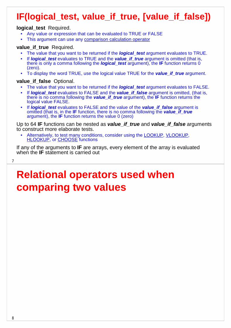
IF(logical_test, value_if_true, [value_if_false])logical_test Required.

• Any value or expression that can be evaluated to TRUE or FALSE• This argument can use any comparison calculation operator

value_if_true Required. • The value that you want to be returned if the logical_test argument evaluates to TRUE. • If logical_test evaluates to TRUE and the value_if_true argument is omitted (that is,

there is only a comma following the logical_test argument), the IF function returns 0 (zero).

• To display the word TRUE, use the logical value TRUE for the value_if_true argument.

value_if_false Optional. • The value that you want to be returned if the logical_test argument evaluates to FALSE. • If logical_test evaluates to FALSE and the value_if_false argument is omitted, (that is,

there is no comma following the value_if_true argument), the IF function returns the logical value FALSE.

• If logical_test evaluates to FALSE and the value of the value_if_false argument is omitted (that is, in the IF function, there is no comma following the value_if_trueargument), the IF function returns the value 0 (zero)

Up to 64 IF functions can be nested as value_if_true and value_if_false arguments to construct more elaborate tests.

• Alternatively, to test many conditions, consider using the LOOKUP, VLOOKUP, HLOOKUP, or CHOOSE functions

If any of the arguments to IF are arrays, every element of the array is evaluated when the IF statement is carried out

8

Relational operators used when comparing two values

9

Using Operators with IF=IF(A1<>A2,"Not Equal","Equal") • If the value of A1 is not the same as the value of

A2, show the words Not Equal; otherwise, show the word Equal

=IF(A1>=0,0,A1)• If the value of A1 is greater than or equal to 0

(zero), show 0; otherwise, show the value of A1

10

Using Operators with IF=IF(IF(A1>A2,200,100)=200,"Yes","No") • If the value of A1 is greater than A2, set a

temporary value to 200; otherwise, set it to 100. Compare the temporary value to 200. If it's equal to 200, display Yes; otherwise, display No

IF(C10=AVERAGE(D1:D5),C10,"Out of Range" • If the average of D1:D5 is equal to C10, show that

average; otherwise, show the text Out of Range

11

IF Examples:If the value of C6 is not equal to the value of

A12 plus 14, display the text "Invalid"; otherwise, display the value of C6

• =IF(C6<>A12+14,"Invalid",C6)

If the value of B4 is greater than the sum of A1:A12, multiply C10 by 1.25; otherwise, multiply C10 by 0.75

• =IF(B4>SUM(A1:A12),C10*1.25,C10*0.75)

12

Nested IF Functions=IF(condition1,expression1,IF(condition2,expression2,expression3))

• If condition1 is true, the relevant value is expression1. Otherwise, condition2 is checked

– If it is true, the relevant value is expression2 Otherwise, the relevant value is expression3

=IF(A1<0,10,IF(A1=0,20,30)) entered in B2• if A1 contains a negative number, B2 contains 10 • Otherwise, if A1 contains 0, B2 contains 20• Otherwise (meaning that A1 must contain a positive

value), B2 contains 30

13

Using Boolean Logical Functions to Evaluate a List of Values and Determine a Single True or False Value

AND Used to determine if all arguments are TRUE

OR Used to determine if either argument is TRUE

NOT Evaluates only one logical argument to determine if it is FALSE

14

AND and OR Truth table

15

Common Logical Constructs

16

IF Functions with Logical AND or OR Conditions

=IF(AND(condition1,condition2),expression1,expression2)• results in expression1 if both condition1 and

condition2 are true• Otherwise, it results in expression2

=IF(OR(condition1,condition2),expression1,expression2)• results in expression1 if either condition1 or

condition2 is true (or if both are true)• Otherwise, it results in expression2

Note that any number of conditions, not just two, could be included in the AND/ OR, all separated by commas

17

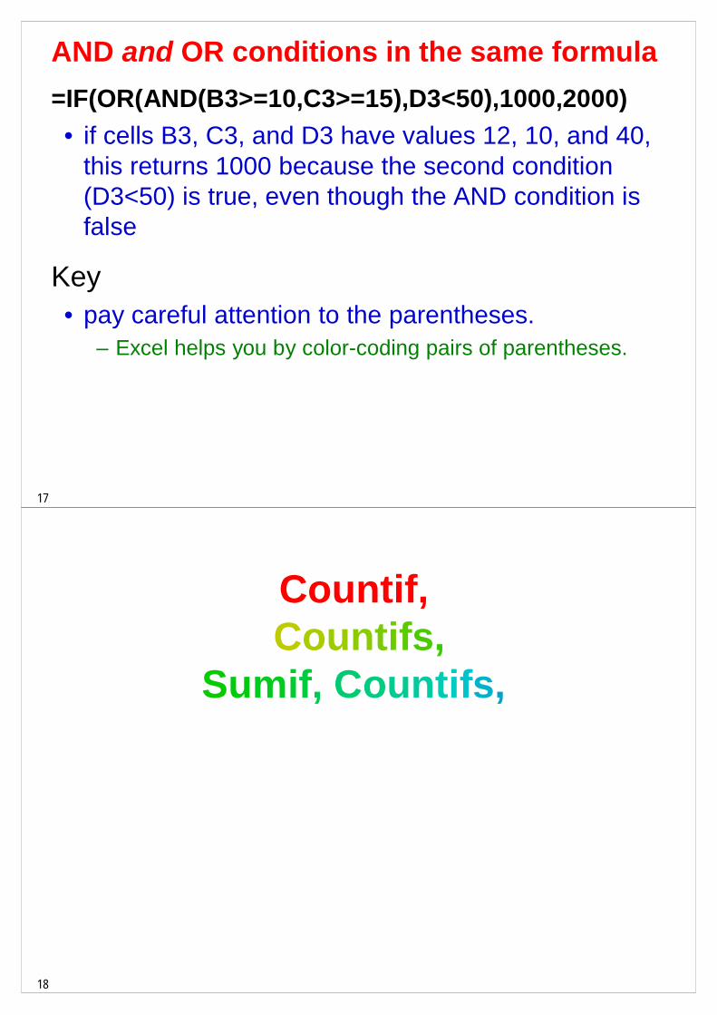
AND and OR conditions in the same formula=IF(OR(AND(B3>=10,C3>=15),D3<50),1000,2000)• if cells B3, C3, and D3 have values 12, 10, and 40,

this returns 1000 because the second condition (D3<50) is true, even though the AND condition is false

Key • pay careful attention to the parentheses.

– Excel helps you by color-coding pairs of parentheses.

18

Countif,Countifs,

Sumif, Countifs,

19

COUNTIF(range, criteria)range Required

• One or more cells to count, including numbers or names, arrays, or references that contain numbers. Blank and text values are ignored.

criteria Required• A number, expression, cell reference, or text string that defines which

cells will be counted. – For example, criteria can be expressed as 32, ">32", B4, "apples", or "32".

Wildcard characters, the question mark (?) and the asterisk (*), can be used in criteria

• A question mark matches any single character, and • An asterisk matches any sequence of characters

– If needed to find an actual question mark or asterisk, type a tilde (~) before the character

• Criteria are case insensitive; – for example, the string "apples" and the string "APPLES" will match the

same cells

20

COUNTIF Function: Examples (1 of 2)=COUNTIF(A1:C12,"?????")

• Counts the number of cells containing exactly five characters of text.

=COUNTIF(A1:C12,100)• Counts the number of cells containing the value 100.

=COUNTIF(A1:C12,"L*")• Counts the number of cells containing text entries that begin with the

letter L

=COUNTIF(A1:C12,">0") • Counts the number of cells containing numeric values greater than zero

=COUNTIF(A1:C12,"<"&B2) • Counts the number of cells containing numeric values less than the

numeric value in cell B2. The comparison operator (<) must be inquotation marks, but the cell reference can't be. The concatenation operator (&) is used to join them

21

COUNTIF Function: Examples (2 of 2)=COUNTIF(A1:C12,">="&MIN(A1:C12))

• Counts the number of cells containing a numeric value greater than or equal to the minimum value in the range

=COUNTIF(A1:C12,TRUE)• Counts the number of cells containing the logical value

TRUE (This is not the same as the text "TRUE")

=COUNTIF(A1:C12,"TRUE")• Counts the number of cells containing the word "TRUE" as

a text entry

=COUNTIF(A1:C12,"<1")+COUNTIF(A1:C12,">10")• Counts the number of cells containing a numeric value less

than 1 and the number of cells containing a numeric value greater than 10, and then adds the two counts

22

Lookup, VLookup,Index, Match

23

Lookup

With Vector form, • it looks for a value in a specified column or row,

– LOOKUP(lookup_value,lookup_vector,result_vector)» lookup_value can be text, number, logical value, a name or a

reference» lookup_vector is a range with only one row or one column

result_vector is a range with only one row or one column

» lookup_vector and result_vector must be the same size

24

Lookup

With Array form, • it looks in the first row or column of an array

– LOOKUP(lookup_value,array)» lookup_value can be text, number, logical value, a name or a

reference» searches based on the array dimensions:» if there are more columns than rows, it searches in the first row» if equal number, or more rows, it searches first column» returns value from same position in last row/column

25

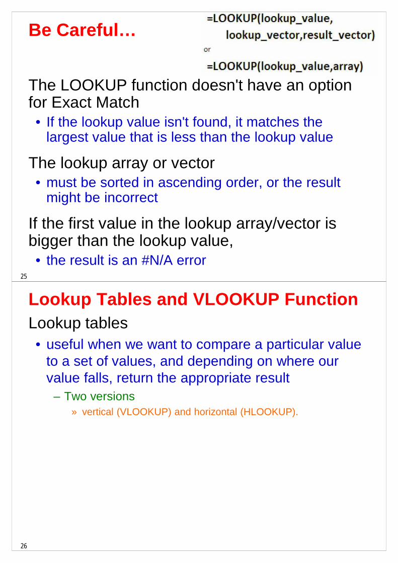
Be Careful…

The LOOKUP function doesn't have an option for Exact Match• If the lookup value isn't found, it matches the

largest value that is less than the lookup value

The lookup array or vector• must be sorted in ascending order, or the result

might be incorrect

If the first value in the lookup array/vector is bigger than the lookup value,• the result is an #N/A error

26

Lookup Tables and VLOOKUP FunctionLookup tables • useful when we want to compare a particular value

to a set of values, and depending on where our value falls, return the appropriate result

– Two versions» vertical (VLOOKUP) and horizontal (HLOOKUP).

27

VLookupVLOOKUP(lookup_value,table_array,col_index_num,range_lookup)

• lookup_value: – the value that you want to look for,

» a value, or a cell reference

• table_array: – the lookup table

» a range reference or a range name, with 2 or more columns

• col_index_num: – the column that has the value you want returned, based

on the column number within the table• [range_lookup]:

– for an exact match, use FALSE or 0; – for an approximate match, use TRUE or 1, with the

lookup value column sorted in ascending order

28

VLOOKUP Function=VLOOKUP(value,lookup table,column #,TRUE or FALSE)• three arguments plus an optional fourth argument:

1. The value to be compared2. A lookup table, with the values to be compared with

always in the left column3. The column number of the lookup table where you find

the “answer”4. TRUE or FALSE (which is TRUE by default if omitted)

29

The optional fourth argument • The default value, TRUE, indicates approximate match

– It sees where the lookup value fits in a range of values, namely, those in the first column of the lookup table.

– the first column of the lookup table must be in ascending order. • if the fourth argument is FALSE, indicates exact match in

the first column of the lookup table. – it doesn't matter whether the first column is in ascending order or

not. – returns an error if no exact match can be found.

Note• Because the VLOOKUP function is often copied down a

column, make the second argument an absolute reference– give the lookup table a range name

» However, a range name is not necessary.

30

Looking Up a Value in a Range (Approx.)Common use of a lookup table is to see where a value fits in a range of values• fourth argument can be omitted, because

– Its default value is TRUE

31

Looking for an Exact MatchRemember three things • The fourth arguments is not optional;

– it must be FALSE• The first column of the lookup table doesn't have to

be in ascending order; – it can be, but order doesn't matter

• If no exact match exists, – the function returns an error (#NA)

32

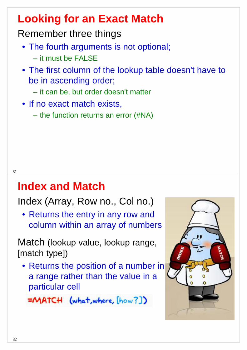
Index and MatchIndex (Array, Row no., Col no.)• Returns the entry in any row and

column within an array of numbers

Match (lookup value, lookup range, [match type])• Returns the position of a number in

a range rather than the value in a particular cell

33

34

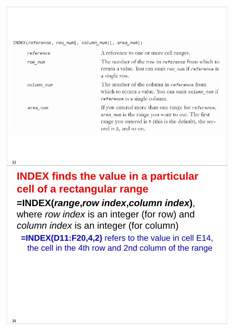
INDEX finds the value in a particular cell of a rectangular range =INDEX(range,row index,column index), where row index is an integer (for row) and column index is an integer (for column)=INDEX(D11:F20,4,2) refers to the value in cell E14,

the cell in the 4th row and 2nd column of the range

35

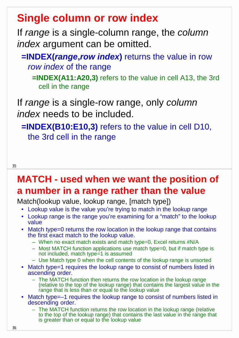
Single column or row indexIf range is a single-column range, the column index argument can be omitted. =INDEX(range,row index) returns the value in row

row index of the range =INDEX(A11:A20,3) refers to the value in cell A13, the 3rd

cell in the range

If range is a single-row range, only column index needs to be included. =INDEX(B10:E10,3) refers to the value in cell D10,

the 3rd cell in the range

36

MATCH - used when we want the position of a number in a range rather than the valueMatch(lookup value, lookup range, [match type])

• Lookup value is the value you’re trying to match in the lookup range• Lookup range is the range you’re examining for a “match” to the lookup

value• Match type=0 returns the row location in the lookup range that contains

the first exact match to the lookup value. – When no exact match exists and match type=0, Excel returns #N/A– Most MATCH function applications use match type=0, but if match type is

not included, match type=1 is assumed– Use Match type 0 when the cell contents of the lookup range is unsorted

• Match type=1 requires the lookup range to consist of numbers listed in ascending order.

– The MATCH function then returns the row location in the lookup range (relative to the top of the lookup range) that contains the largest value in the range that is less than or equal to the lookup value

• Match type=–1 requires the lookup range to consist of numbers listed in descending order.

– The MATCH function returns the row location in the lookup range (relative to the top of the lookup range) that contains the last value in the range that is greater than or equal to the lookup value

37 37

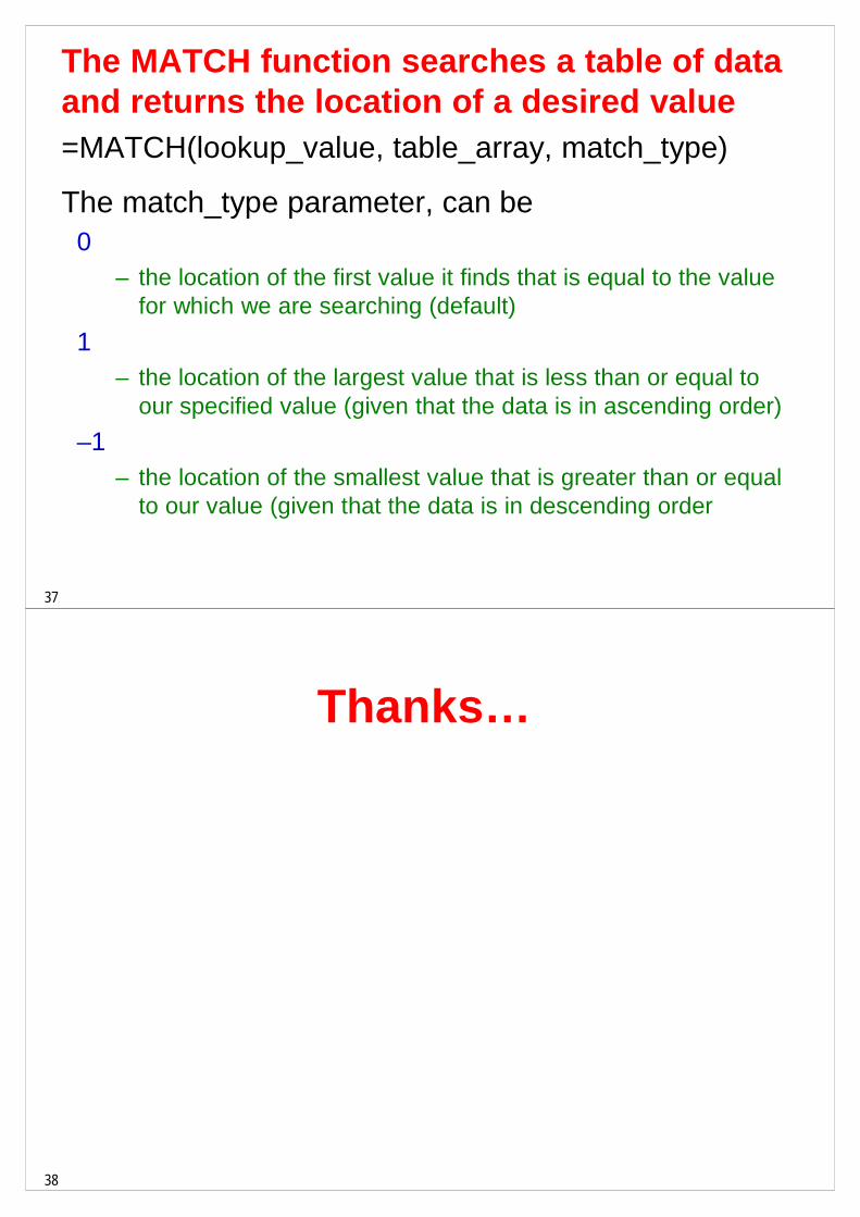
The MATCH function searches a table of data and returns the location of a desired value=MATCH(lookup_value, table_array, match_type)

The match_type parameter, can be0

– the location of the first value it finds that is equal to the value for which we are searching (default)

1– the location of the largest value that is less than or equal to

our specified value (given that the data is in ascending order)–1

– the location of the smallest value that is greater than or equalto our value (given that the data is in descending order

38

Thanks…