on june 11, 2018 artsofelectricalimpedance...

rsta.royalsocietypublishing.org

ResearchCite this article:Wang M, Wang Q, Karki B.2016 Arts of electrical impedance tomographicsensing. Phil. Trans. R. Soc. A 374: 20150329.http://dx.doi.org/10.1098/rsta.2015.0329

Accepted: 14 March 2016

One contribution of 10 to a theme issue‘Super-sensing through industrial processtomography’.

Subject Areas:electromagnetism, optics, electricalengineering, computer vision, chemicalengineering, mechanical engineering

Keywords:electrical impedance tomography, sensitivity,resolution matrix, regional imaging withlimited measurements

Author for correspondence:Mi Wange-mail: [email protected]

Arts of electrical impedancetomographic sensingMiWang, Qiang Wang and Bishal Karki

School of Chemical and Process Engineering, University of Leeds,Leeds, West Yorkshire LS2 9JT, UK

This paper reviews governing theorems in electricalimpedance sensing for analysing the relationships ofboundary voltages obtained from different sensingstrategies. It reports that both the boundary voltagevalues and the associated sensitivity matrix of analternative sensing strategy can be derived from aset of full independent measurements and sensitivitymatrix obtained from other sensing strategy. A newsensing method for regional imaging with limitedmeasurements is reported. It also proves that thesensitivity coefficient back-projection algorithm doesnot always work for all sensing strategies, unlessthe diagonal elements of the transformed matrix,ATA, have significant values and can be approximateto a diagonal matrix. Imaging capabilities of fewsensing strategies were verified with static set-ups,which suggest the adjacent electrode pair sensingstrategy displays better performance compared withthe diametrically opposite protocol, with both theback-projection and multi-step image reconstructionmethods. An application of electrical impedancetomography for sensing gas in water two-phase flowsis demonstrated.

This article is part of the themed issue ‘Super-sensing through industrial process tomography’.

1. IntroductionElectrical tomography, including the measurement basedon electrical property, e.g. electrical impedance tomo-graphy (EIT) or dielectric property, e.g. electricalcapacitance tomography (ECT), has been developedsince the late 1980s to provide alternative, low-costsolution for clinical, geophysical and industrial processapplications [1]. A number of sensing strategies forEIT have been developed in previous years. The most

2016 The Authors. Published by the Royal Society under the terms of theCreative Commons Attribution License http://creativecommons.org/licenses/by/4.0/, which permits unrestricted use, provided the original author andsource are credited.

on July 10, 2018http://rsta.royalsocietypublishing.org/Downloaded from

http://crossmark.crossref.org/dialog/?doi=10.1098/rsta.2015.0329&domain=pdf&date_stamp=2016-05-16

http://dx.doi.org/10.1098/rsta/374/2070

mailto:[email protected]

http://creativecommons.org/licenses/by/4.0/

http://creativecommons.org/licenses/by/4.0/

http://rsta.royalsocietypublishing.org/

2

rsta.royalsocietypublishing.orgPhil.Trans.R.Soc.A374:20150329

.........................................................

common choices were four-electrodes measurement, e.g. the adjacent electrode pair protocol [2]and diametrically opposite protocol [3] in EIT, or three-electrodes measurement, e.g. the metalwall protocol [4] in EIT and that used in most of ECT systems [5,6]. However, there is as yetno general agreement for the ‘best’ sensing strategy in this area [7]. Based on the reciprocityand sensitivity theorem proved by Geselowiz [8] and Lehr [9] and the assumption cited forsensitivity coefficient back-projection (SBP) approximation [10], the principles of reciprocity andindependency and also imaging capability in EIT are discussed in this paper.

2. Governing theorems

(a) Lead theorem and reciprocity theoremThe lead theorem was derived from the divergence theorem (equation (2.1)) by Geselowitz [8]and Lehr [9] for the impedance plethysmography.∫

Ω

∇ · A dΩ =∮

SA · dS, (2.1)

where Ω is a region bounded by a closed surface S. A is a vector function of the position.The mutual impedance Z of a four-electrode system with a known conductivity distribution

can be derived by substituting ψJφ or φJψ into the divergence theorem (equation (2.1)) and thensubstituting Jφ = −σφ∇φ or Jψ = −σψ∇ψ into the left side of the reformed expression under thecondition of no internal current source [4], where ψ and φ are potential distributions in responseto the presence of currents Iψ and Iφ at two ports (A–B and C–D), respectively.

Z = φAB

Iφ= ψCD

Iψ=

∫Ω

σ∇φIφ

· ∇ψIψ

dΩ . (2.2)

The mutual impedance change �Z owing to a change of internal conductivity �σ for a four-electrode system, derived by Geselowits and Lehr and later linearized by Murai & Kagawa [11],is given as equations (2.3) and (2.4), respectively. Equation (2.4) ignores the high-order term andprovides a linear relationship with an assumption of �σ � σ . Equations (2.2) and (2.3) are alsocalled the reciprocity theorem.

�Z = �φAB

Iφ= �ψCD

Iψ= −

∫Ω

�σ∇φΞ

Iφ· ∇ψ

IψdΩ , (2.3)

where φΞ is the potential change caused by the conductivity after change σΞ = σ +�σ

�Z = −∫Ω

�σ∇φIφ

· ∇ψIψ

dΩ + 0((�σ )2) ≈ −∫Ω

�σ∇φIφ

· ∇ψIψ

dΩ (�σ � σ ). (2.4)

(b) Sensitivity theoremSupposing that the conductivity distribution is composed of w small uniform ‘patches’ or pixels,then equations (2.2) and (2.4) can be expressed as equations (2.5) and (2.6) and the sensitivitycoefficient s for each discrete pixel is given by equation (2.7) [11–13].

�Z =w∑

k=1

�σksφ,ψ ,k, (2.5)

Z =w∑

k=1

�σksφ,ψ ,k (2.6)

and sφ,ψ ,k(σk) = −∫Ωk

∇φIφ

· ∇ψIψ

dΩk, (2.7)

where Ωk stands for a discrete two-dimensional area at location k; σk and �σk denote theconductivity and the change of conductivity Ωk, respectively.



3


.........................................................

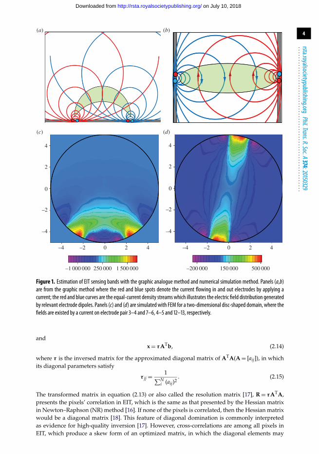
Equation (2.7) indicates that the sensitivity at a defined location is a vector scalar productionof two electrical fields generated by current excitations on source and measurement electrodepairs (equation (2.7)). In other words, the sensitivity will be maximized at a location whentwo electric fields are mostly in parallel. With the orthogonal principle between the electricalpotential and current density (electrical field intensity) of two electric dipoles, figure 1 illustratesthe sensing ‘bands’ produced by two pairs of electrodes positioned on a non-conductive plateand an opposite position, respectively. The graphic method (figure 1a,b) is a simple way toinitially estimate the sensitive region from a setting up of electrode allocation for process vesselshaving different geometry, where the sensing ‘bands’ are highlighted in green. However, no sharpboundary of bands exists in an actual sensitivity distribution owing to the use of low-frequencyelectromagnetic excitation. In practice, the sensitivity coefficients are normally computed witheither analytical or numerical methods. Figure 1c,d demonstrates the sensitivity distributionssimulated with finite-element modelling method (FEM) for a 16-electrode sensing array, wherefigure 1c is generated by excitation and measurement electrode pairs 3–4 and 7–6 and figure 1dis from electrode pair 4–5 and 12–13. For a good sensing strategy, it is necessary the coveragescanning and cross-band scanning can be made over the domain of interests.

(c) Inverse solutionFor a linear equation (2.8), the minimization function (2.10) can be obtained from minimizingequation (2.9).

A · x = b, (2.8)

f (x) = 12 ‖Ax − b‖2 (2.9)

and ∇f (x) = AT(Ax − b). (2.10)

Let ∇f = 0, then,

ATAx = ATb. (2.11)

If an inverse matrix of ATA exists, then the solution can be made as equation (2.12)

x = (ATA)−1ATb. (2.12)

It is known the inverse matrix of ATA is not derivable owing to the ill condition of sensitivitymatrix A in EIT. Many indirect methods were developed to solve the linear equation in thepast. Typically, they were reported as the back-project method [14] and the Newton one-stepreconstruction (NOSER) single step method [15]. However, it should be pointed out the solutionfor equation 2.12, if any exists, only satisfies the change of conductivity �σ � σ . The closestsolution may only be obtained from multi-step approach [16].

(i) Back-projection methods

Wang [10] indicated that the sensitivity coefficient back-projection method (SBP) is actuallybased on an assumption of that the diagonal elements of the transformed matrix, ATA, havethe most significant values and the matrix can be approximate to a diagonal matrix. For aparticular example of adjacent sensing strategy, the solution to equation (2.10)) with ∇f = 0 isfirstly normalized to equation (2.13), then approximate to equation (2.14) if the τATA can beapproximated as an identity matrix.

τATAx = τATb (2.13)



4


.........................................................

4

2

0

–2

–4

4

2

0

–2

–4

–4 –2

–1 000 000 250 000 1 500 000 –200 000 150 000 500 000

0 2 4 –4 –2 0 2 4

(a) (b)

(c) (d)

Figure 1. Estimation of EIT sensing bands with the graphic analogue method and numerical simulation method. Panels (a,b)are from the graphic method where the red and blue spots denote the current flowing in and out electrodes by applying acurrent; the red and blue curves are the equal-current density streams which illustrates the electric field distribution generatedby relevant electrode dipoles. Panels (c) and (d) are simulated with FEM for a two-dimensional disc-shaped domain, where thefields are existed by a current on electrode pair 3–4 and 7–6, 4–5 and 12–13, respectively.

andx = τATb, (2.14)

where τ is the inversed matrix for the approximated diagonal matrix of ATA(A = [aij]), in whichits diagonal parameters satisfy

τ jj = 1∑Ni (aij)2

. (2.15)

The transformed matrix in equation (2.13) or also called the resolution matrix [17], R = τATA,presents the pixels’ correlation in EIT, which is the same as that presented by the Hessian matrixin Newton–Raphson (NR) method [16]. If none of the pixels is correlated, then the Hessian matrixwould be a diagonal matrix [18]. This feature of diagonal domination is commonly interpretedas evidence for high-quality inversion [17]. However, cross-correlations are among all pixels inEIT, which produce a skew form of an optimized matrix, in which the diagonal elements may



5


.........................................................

resolution matrix

2.51.50.5

–0.5–1.5

0

50

100

150

200

0

50

100

150

200

col

row

Figure 2. Resolution matrix for a 16-electrode sensing array using the adjacent electrode pair sensing strategy with a two-dimensional mesh with 224 pixels.

have most significant values. Figure 2 demonstrates the significance of diagonal components inthe resolution matrix from the adjacent electrode pair sensing strategy, which are modelled usingFEM with a mesh having 224 pixels for a 16-electrode sensing array. Equation (2.14) with theexistence of the diagonal matrix approximation provides the mathematical principle for the SBPalgorithm.

(ii) Multi-step methods

The linear approximation, based on ignoring the high-order terms with respect to �σ � σ (seeequation (2.4)), enables the use of iterative techniques to solve the linear equation (equation (2.11))with a pre-calculated sensitivity matrix based on an estimated initial conductivity distribution,e.g. a homogeneous distribution. However, in most of cases, multi-steps of the linear solutionprocess have to be applied in order to achieve better image quality, where the sensitivity matrixshould be updated with the change of conductivity distribution obtained from the previousstep. Its performance is strongly associated with the methods and the convergent factors usedin iterative minimization process as given by equation (2.16). The typical examples are the use ofNR optimization [16], Tikhonov regularization method [19,20] with the techniques of selection ofregularization factors such as the singular value decomposition method and Akaike’s informationcriterion [21] and the Marquardt method [22].

The error function is

r = τATAx − τATb. (2.16)

(iii) One-step methods

One-step method refers the solution from the iterations at the end of the first step of a multi-step method. It is the fact that the result from the first-step solution normally provides themost contributive convergence if the regularization factors are properly selected. The quality ofresultant images is generally much better than those came from back-projection approximationas results from NOSER method [15] and the SCG method [10]. It also runs at a much fast speedthan that of multi-step method owing to the use of the pre-calculated sensitivity matrix. Aniterative solution can be obtained in a kind of the Landweber iteration method as expressed by



6


.........................................................

Em

CH

Rc

Rb

bulk resistance

A

V

d

l

r

(a) (b)

Figure 3. (a) The electrode–electrolyte interface; (b) four-electrode method. (Online version in colour.)

equation (2.17) [23].xn ≈ xn−1 − rn = xn−1 − τAT(Axn−1 − b). (2.17)

The selection of τ for the SBP has been suggested by equation (2.15). An example for the use ofLandweber’s method with selection of τ for capacitance tomography was reported by Liu et al.[24] and also many other recent publications. For a general application, the selection of τ can bereferred from the Landweber method [23].

3. Sensing strategy

(a) Electrode–electrolyte interfaceA metal electrode immersed in an electrolyte is polarized when its potential is different from itsopen-circuit potential [25]. The electrode used in EIT is a transducer that converts the electroniccurrent in a wire to an ionic current in an electrolyte. The behaviour at the electrode–electrolyteinterface is a predominantly electrochemical reaction [26]. The electrode–electrolyte interface canbe described by a simple circuit as shown in figure 3a, where RC denotes the charge transferresistance, CH represents the double layer capacitance, Em is the over potential difference andRb is the bulk resistance of a process. All of these three major representatives are function of theionic concentration of the electrolyte, surface area and condition of electrode, and also currentdensity over the interface. The conventional and effective way to avoid error caused by theinterface in the measurement of bulk resistance is to use a four-electrode method as shown infigure 3b. In principle, the voltage measurement, V, should not be a function of the two interfaces’electrochemical characteristics because the current, I, remains constant flowing through any crosssection of the cylindrical object. The four-electrode method is also widely used in EIT [1], typically,as it is used in adjacent electrode pair sensing strategy.

(b) Sensing strategiesIn EIT, the boundary conditions required to determine the electrical impedance distribution ina domain of interest comprise the injected currents via electrodes and subsequently measuredvoltages, also via boundary electrodes. A number of excitation and measurement methods orsensing strategies have been reported since the late 1980s [1,27]. Figure 4 shows three differentsensing strategies under the review, which are adjacent electrode pair strategy [2] (figure 4a),an alternative sensing strategy (figure 4b), which is named as PI/2 protocol owing to a π/2radian between its nearest measurement electrode pairs [28], and the diametrically oppositesensing strategy [3] (figure 4c). Applying the reciprocity theorem or leads theorem as given byequations (2.2) and (2.3) and also in the use of four-electrode method, the number of independentmeasurements from these strategies (ignoring the measurements from current drive electrodes) is104, 72 and 96, respectively.



7


.........................................................

1

2

34

5 67

8

9

10

11

121314

1516

V

1

2

3

45 6

7

8

9

10

11

121314

1516

V

1

2

3

45 6

7

8

9

10

1112

131415

16

V(a) (b) (c)

Figure 4. Different sensing protocols: (a) adjacent sensing strategy, (b) PI/2 sensing strategy, (c) opposite sensing strategy.

(c) Linear relationshipsTaking the example of the measurement and excitation positions in the PI/2 sensing strategy(figure 4b), its boundary voltages can be derived from the adjacent electrode pair sensing strategybased on the theorem of circuitry. Firstly, we have

V6,9(I1,2) = V6,7(I1,2) + V7,8(I1,2) + V8,9(I1,2)

and Z6,9(I1,2) = Z6,7(I1,2) + Z7,8(I1,2) + Z8,9(I1,2)

}(3.1)

where V6,9(I1,2) denotes the voltage measured from the electrode 6 and 9 when a current presentedbetween the electrode 1 and 2, Z6,9(I1,2) represents the mutual impedance, V6,9/I1,2.

According to the reciprocity theorem, the mutual impedance can be expressed as

Z1,2(I6,9) = Z6,9(I1,2)

Z2,3(I6,9) = Z6,9(I2,3)

and Z3,4(I6,9) = Z6,9(I3,4).

⎫⎪⎪⎬⎪⎪⎭ (3.2)

Following the principles of equations (2.2) and (2.4), the mutual impedance of the circuitry infigure 1b can be presented as

Z1,4(I6,9) = Z1,2(I6,9) + Z2,3(I6,9) + Z3,4(I6,9) = Z6,9(I1,2) + Z6,9(I2,3) + Z6,9(I3,4). (3.3)

Substituting equation (3.1) into equation (3.3) with the reciprocity given by equation (2.4), themutual impedance of the circuitry in figure 4b can be described using a set of the mutualimpedances derived from the circuitry in figure 4a

Z6,9(I1,4) = Z1,4(I6,9) = Z6,7(I1,2) + Z7,8(I1,2) + Z8,9(I1,2)

+ Z6,7(I2,3) + Z7,8(I2,3) + Z8,9(I2,3) (3.4)

+ Z6,7(I3,4) + Z7,8(I3,4) + Z8,9(I3,4).

Further, the boundary voltages in figure 4b can be expressed with a set of boundary voltages ofthe circuitry in figure 1a.

if I1,4 = I6,9 = I1,2 = I2,3 = I3,4

V6,9(I1,4) = V1,4(I6,9) = V6,7(I1,2) + V7,8(I1,2) + V8,9(I1,2) (3.5)

+ V6,7(I2,3) + V7,8(I2,3) + V8,9(I2,3)

+ V6,7(I3,4) + V7,8(I3,4) + V8,9(I3,4).

A general form of the relationship between an alternative four-electrode sensing strategy andthe adjacent sensing strategy in EIT can be expressed as equation (3.6), which derives a mutual



8


.........................................................

impedance or a boundary voltage for an alternative four-electrode sensing strategy from a set ofmutual impedances of the adjacent electrode pair strategy.

ZI,J(IM,N) =N−1∑m=M

J−1∑i=I

Zi,i+1(Im,m+1) (M<N< I< J), (3.6)

where M and N denote the current drive electrode pair, I and J denotes the measurement electrodepair of the alternative four-electrode sensing strategy.

Because a linear approximation has been adopted in the calculation of sensitivity matrix[8,9,11] and a linear relationship of the boundary voltages exists for different four-electrodesensing strategies (equation (3.6)), the sensitivity matrix of an alternative sensing strategy can alsobe derived from the sensitivity matrix obtained from a complete set of independent measurementsof other sensing strategy. Equation (3.7) gives the derivation from the sensitivity matrix of theadjacent electrode strategy.

sI,J(IM,N) =N−1∑m=M

J−1∑i=I

si,i+1(Im,m+1) (M<N< I< J). (3.7)

(d) Regional imaging based on reduced measurementsThe characteristics of multi-phase pipeline flow, such as disperse phase concentration and velocitydistributions, can be assumed as either radial symmetrical in vertical pipeline or central–verticalplane symmetrical in horizontal pipeline. The necessary and minimum imaging area, which canrepresent the major features of pipeline flows when both cases are combined, is the columnsof pixels along the central–vertical plane, as indicated in figure 5. Therefore, targeting only thecentral one or few columns of the full tomogram as shown in figure 5 will result in lesser numberof measurements thereby increasing the speed while maintaining the spatial resolution to acomparable level. A new sensing strategy, based on 16-electrode EIT, called regional imagingwith limited measurements (RILM) was developed in order to achieve similar performanceto the conventional EIT sensing protocol but using limited measurements [30]. The selectionof measurements can be based on the analysis of sensing regions by either the graphic ornumerical simulation as shown in figures 1 and 2, respectively. Alternatively, by analysing thepixel sensitivity matrix, S = τAT, the sensitive level of pixel’s conductivity owing to the changeof boundary measurements can be obtained (figure 6), which provides an analytical method forthe implementation of RILM. In the practice, the selection starts with the graphic method wouldbe mostly effective.

The sensing strategy of the RILM consists of three groups of excitation and measurementelectrode pairs arranged in rotary, parallel and complimentary positions as shown in figure 7a,band c, respectively. Each projection is carried out by applying current to a pair of electrodes andmeasuring voltage from other pair of electrodes corresponding to the electrode pairs adjacent tothe terminals of each rectangular bar in figure 7. A total of 20 measurements, i.e. eight for rotary,six for parallel and seven for complimentary position are required to focus the sensitivity in thecentral region as illustrated in figure 7d,e based on the reciprocity theorem.

Further experiments were conducted using the air–water two-phase upward flow in verticalpipeline with inner diameter of 50 mm at the University of Leeds. Slug flow regime was testedwith water and air flowing at 27 rpm and 70 litre min−1, respectively. A fast 16-electrode EITsystem (FICA) was used to collect data at a speed of 1000 dual frames per second. Data for RILMwere extracted from the full set of measured data, and velocity and concentration profiles weregenerated in both cases.

Stacked images of two-phase slug flow, reconstructed from full measurement, and RILMmeasurement are shown in figure 8. Average of the central four rows of the tomograms was usedin the stacked images. RILM was able to produce comparable visualization with respect to fullmeasurement.



9


.........................................................

12

34

56

98

7

1718

1920

1011

1213

1415

16

2122

2324

2526

2728

2930

3231

3334

3536

3738

3940

4142

4344

4546

4847

4950

5152

5354

5556

5758

5960

6162

6564

6366

6768

6970

7172

7374

7576

7778

7980

8382

8184

8586

8788

8990

9192

9394

9596

9798

102

101

100

9910

310

410

510

610

710

810

911

011

111

211

311

411

511

611

711

8

122

121

120

119

123

124

125

126

127

128

129

130

131

132

133

134

135

136

137

138

142

141

140

139

143

144

145

146

147

148

149

150

151

152

153

154

155

156

157

158

162

161

160

159

163

164

165

166

167

168

169

170

171

172

173

174

175

176

177

178

179

180

181

182

183

184

185

186

187

188

189

190

191

192

193

194

195

196

197

198

199

200

201

202

203

204

205

206

207

208

209

210

211

212

213

214

215

216

217

219

220

221

222

223

224

225

226

227

228

229

230

231

232

233

234

235

236

237

238

239

240

241

242

243

244

245

246

247

248

249

250

251

252

253

255

256

257

258

259

260

261

262

263

264

265

266

267

268

269

270

271

272

273

274

275

276

277

278

279

280

281

282

283

284

285

287

288

289

290

291

292

293

294

295

296

297

298

301

302

303

304

305

306

307

308

311

312

313

314

315

316

309

310

299

300

286

254

218

Figure 5. The central columns with 80 elements in the arrangement of 316 tomogram elements by 20 × 20 grid [29]. (Onlineversion in colour.)

The concentration and velocity profiles were obtained from full measurement as well as RILMfor air–water upward two-phase flow in vertical pipeline are illustrated in figure 9a and b,respectively. The profiles were calculated from the mean value of reconstructed tomograms.Similar characteristics are demonstrated by the profiles obtained from both strategies. Thedifference between them is more pronounced towards the boundary than the centre of the pipe.

Because RILM requires considerably lesser number of measurements, it is reasonable toanticipate that RILM could outperform conventional EIT systems in terms of measurement speedand communication rate.

4. Imaging capability

(a) Set-upsAs discussed in §3d, the boundary voltages and the sensitivity matrix for an alternative sensingstrategy can be derived from a complete set of independent measurements (equations (3.6) and(3.7)). Therefore, from the algebraic principle, no new information could be obtained from suchan arithmetic combination. In practice, the image sensitivity, accuracy and spatial resolutioncould be affected by the actual signal-to-noise ratio (SNR) and sensitivity distribution of an



10


.........................................................

sensitivity matrix

4 ¥ 10–7

2 ¥ 10–7

–7 ¥ 10–8

–3 ¥ 10–70

50

100

150

200

row

0

50

100

col

Figure 6. The pixel sensitivity matrix created using FEM with a two-dimensional mesh with 224 triangle pixels for 104independent measurements from a 16-electrode sensor using adjacent electrode pair sensing strategy. Each row of the matrixcontains 104 coefficients, which reports the sensitivity of pixel value in correspondence to measurements.

54

3

2

1

16

15

1412

11

10

9

8

7

6

13

5 4

3

2

1

16

15

1412

11

10

9

8

7

6

13

54

3

2

1

16

15

1412

11

10

9

8

7

6

13

5 4

3

2

1

16

15

1412

11

10

9

8

7

6

13

54

3

2

1

16

15

1412

11

10

9

8

7

6

13

(a) (b) (c)

(d) (e)

Figure 7. RILM sensing strategy, (a) rotary band, (b) parallel band and (c) complimentary band, (d) overall projections and(e) region of high sensitivity.

alternative sensing strategy. To reveal features of the differences, three set-ups of FEM elementaryconductivity as defined in figure 10 were employed, in which a low conductive ‘object’ was‘moved’ from the centre to the side of the domain.



11


.........................................................

cent

ral

axia

l pix

els 20

15105

100 200 300 400 500 600 700 800 900 1000

100 200 300 400 500no. frames

600 700 800 900 1000

1.0

0.5

0

1.0

0.5

0

cent

ral

axia

l pix

els 20

15105

Figure 8. Stacked image of two-phase flow: the top image from full measurement, the bottom image from RILM, where theflowing direction is from the right to left; the red and blue colours in the colour palettes on the right ends of images indicatethe volume fraction of air, representing the air and water, respectively.

60 3.0

2.5

2.0

1.5

1.0

0.5

0

50

40

conc

entr

atio

n (%

)

velo

city

(m

s–1)

30

20

10

0–0.06 0.060.04

full measurementRILM

0.02–0.04 –0.02 0pipe diameter (m)

–0.06 0.060.040.02–0.04 –0.02 0pipe diameter (m)

(a) (b)

Figure 9. (a) Concentration profile, (b) velocity profile of air–water vertical flow.

object: 0.011 ms cm–1background: 0.11 ms cm–1

N0

N8

N16

N24

opposite

PI/2

adj.

p1

p2

p3

adj.

Figure 10. FEM set-ups.

(b) Imaging capabilityImages in figure 11a–c were reconstructed using the sensitivity theorem-based inverse solution(SCG) [10]. The images obtained from SCG took five iterative steps and 12 iterations for eachinverse step. All strategies have a convergent error reduction. The adjacent strategy gives themaximum sensitivity (boundary voltage changes) from these conductivity set-ups and highestconvergence speed in the three strategies. The conventional SBP algorithm was also employed to



12


.........................................................

(a) (b) (c) (d) (e) ( f )

Figure 11. Reconstructed images from the simulated data obtained from adjacent (a,d), PI/2 (b,e) and opposite sensing (c,f )strategies for different conductivity set-ups, p1, p2, p3, as given in figure 9. Images were reconstructed using SCG (a–c) and SBPmethods (d–f ).

reconstruct the images using the original boundary voltages and sensitivity matrixes of regardedsensing strategy. Significant differences in imaging quality of the three strategies are shown infigure 11d–f . Comparing the results obtained with SCG algorithm, it is obvious that the differenceis due to the diagonal matrix approximation in SBP method. Different imaging qualities have beenreached from these results. Images obtained from the adjacent electrode pair strategy have shownthe best quality. The poorest quality, particularly at the central region, was delivered from theopposite strategy although the number of measurements (96) in opposite strategy almost closes tothe number of measurements from adjacent strategy (104). The images from PI/2 were quite goodconsidering its limited number of measurements (72). It is well known that the quality of resultantimage is based on the quantity of acquired information. The quality decay of the image here maybe caused by the reduction of information quantity and the ill-conditioned sensitivity matrix,because no noise has been introduced in the simulation. Employing equation (3.4) to analyse theopposite strategy, it can be seen that a large number of repeated basic measurements are involvedin the combination. As we discussed in §3d, the applicability of SBP depends on the physicalfeature of the sensing strategy and whether its diagonal elements of the resolution matrix, τATA,have the most significant values and therefore can approximate to a diagonal matrix. The imagingquality will highly depend on the feature. Therefore, the SBP is, in general, not applicable to allsensing strategies.

5. Imaging of gas–water flowsA considerate set of experiments has been carried out at National Engineering Laboratory inindustry-scale experimental flow facilities for the purpose of evaluating electrical tomographytechnology for new generation of metrology. The pipeline with diameter of 4 inches washorizontally positioned, and the measurement points were located approximately 50 m fromthe injection points, resulting in fully developed multi-phase flows. Nitrogen, oil with viscosity19.4 × 10−6 m2 s−1, and salty water were used as the fluids, with the pressure up to 10 bars. Theexperiment covered water-cuts with the range of [0%, 100%], combined with gas volume fractionof [0%, 100%], and the flowrate for every phase is 0–140 m3 h−1. This thorough experimentmanaged to produce all common flow regimes for horizontal flow, including (wavy) stratifiedflow, plug flow, slug flow, bubbly flow and annular flow.

Accordingly, figure 11 demonstrates only the visualization results for gas–water two-phaseflow using voltage-driven EIT system [31]. The flows are visualized with different flow conditions



13


.........................................................

0 0.250 0.500concentration

0.750 1.000

0 0.250 0.500concentration

0.750 1.000

concentration0 0.250 0.500 0.750 1.000

concentration0 0.250 0.500 0.750 1.000

(a)

(b)

(c)

(d)

Figure 12. Accumulated axial stacked images of different flow patterns, (a) wavy stratified flow (vgas = 39.58 and vliquid =2.08 l s−1), (b) bubbly flow (vgas = 2.05 and vm = 38.89 l s−1), (c) plug flow (vgas = 4.17 and vliquid = 23.61 l s−1), (d) slugflow (vgas = 16.67 and vliquid = 11.11 l s−1). The flow direction is from the right to left.

by means of accumulating diameter-direction pixels of cross-sectional concentration tomogramsfrom 2000 frames to form axial cross-sectional stacked images. From flow pattern point of view,figure 11 also indicates different flow regimes, including stratified flow (figure 12a), bubbly flow(figure 12b), plug flow (figure 12c) and slug flow (figure 12d).

6. Discussion and conclusionThe linear relationship between alternative four-electrode sensing strategies exists. The boundaryvoltages and the sensitivity matrix for an alternative four-electrode sensing strategy can bederived from a complete set of independent measurements. The sensitivity matrix for aspecific distribution can also be derived from either an alternative sensing strategy or a



14


.........................................................

particular combination of the sensitivity matrix derived from a known basic set of independentmeasurements. From algebraic principles, no new information or great accuracy could beobtained from such an arithmetic combination. In practice, the image sensitivity, accuracy andspatial resolution could be affected from the actual SNR and sensitivity distribution achieved fromthe alternative sensing strategy. The results of the derivation imply that the imaging sensitivitycan be relatively intensified or attenuated at a particular area of interest by manipulation ofmatrixes. The applicability of a back-projection algorithm depends on the specific feature ofthe resolution matrix, τATA, which is generally determined by the sensing strategy although itcan be revised later owing to the linear relationship between four-electrode sensing strategies.Applicability of back-projection (e.g. SBP) is subject to whether its diagonal elements of thetransformed matrix, ATA, have the most significant values, and the matrix can approximateto a diagonal matrix. Therefore, the SBP is, in general, not applicable to all sensing strategies.Based on the electrical tomography principle and its sensitivity analysis, electrical tomographyimaging may ‘focus’ on part (or sector) of the conventional full image. Based on the methodof analysing the pixel sensitive matrix, τAT, the boundary voltage contribution to each pixelvalue can be estimated. A specific method, RILM for imaging of a vertical multi-phase flow isdemonstrated, which only uses 20 measurements comparing the conventional 104 measurements.Because RILM requires considerably lesser number of measurements, it is reasonable to anticipatethat RILM could outperform conventional EIT systems in terms of measurement speed andcommunication rate.

The clarifications and expressions on the theories of the back-projection method, the linearrelationships between sensing strategies and sensitivity matrixes, as well as the RILM have thepotential to enhance imaging sensitivity by manipulation of matrixes and to extend electricaltomography to specific applications.

Competing interests. We declare we have no competing interests.Funding. This work is funded by the Engineering and Physical Sciences Research Council (EP/H023054/1, IAA(ID101204) and the European Metrology Research Programme (EMRP) project ’Multiphase flow metrology inthe Oil and Gas production’, which is jointly funded by the European Commission and participating countrieswithin Euramet and the European Union.

References1. Wang M. 2015 Industrial tomography: systems and application, ch. 2 (ed. M Wang), 1st edn.

Cambridge, UK: Woodhead Publishing.2. Brown BH, Barber DC, Seagar AD. 1985 Applied potential tomography: possible clinical

applications. Clin. Phys. Physiolog. Meas. 6, 109–121. (doi:10.1088/0143-0815/6/2/002)3. Hua P, Webster JG, Tompkins WJ. 1987 Effect of the measurement method on noise handing

and image quality of EIT imaging. Proc. Annu. Int. Conf. IEEE Eng. In Med. Biol. Soc. 9,1429–1430.

4. Wang M, Dickin FJ, Williams RA. 1995 Modelling and analysis of electrically conductingvessels and pipelines in electrical resistance process tomography. IEE Proc. Sci. Meas. Technol.142, 313–322. (doi:10.1049/ip-smt:19951923)

5. Huang SM, Plaskowski AB, Xie CG, Beck MS. 1989 Tomographic imaging of two-component flow using capacitance sensors. J. Phys. E, Sci. Instrum. 22, 173–174. (doi:10.1088/0022-3735/22/3/009)

6. Yang WQ. 1996 Hardware design of electrical capacitance tomography systems. Meas. Sci.Technol. 7, 225–232. (doi:10.1088/0957-0233/7/3/003)

7. Boone K, Barber D, Brown B. 1997 Review imaging with electricity: report of theEuropean concerted action on impedance tomography. J. Medical Eng. Technol. 21, 201–232.(doi:10.3109/03091909709070013)

8. Geselowitz DB. 1971 An application of electrocardiographic lead theory to impedanceplethysmography. IEEE Trans. Biomed. Eng. 18, 38–41. (doi:10.1109/TBME.1971.4502787)

9. Lehr J. 1972 A vector derivation useful in impedance plethysmographic field calculations.IEEE Trans. Biomed. Eng. 19, 156–157. (doi:10.1109/TBME.1972.324058)


http://dx.doi.org/doi:10.1088/0143-0815/6/2/002

http://dx.doi.org/doi:10.1049/ip-smt:19951923




http://dx.doi.org/doi:10.3109/03091909709070013

http://dx.doi.org/doi:10.1109/TBME.1971.4502787



15


.........................................................

10. Wang M. 2002 Inverse solutions for electrical impedance tomography based on conjugategradients methods. Meas. Sci. Technol. 13, 101–117. (doi:10.1088/0957-0233/13/1/314)

11. Murai T, Kagawa Y. 1985 Electrical impedance computed tomography based on a finiteelement model. IEEE Trans. Biomed. Eng. 32, 177–184. (doi:10.1109/TBME.1985.325526)

12. Breckon WR, Pidcock MK. 1987 Mathematical aspects of impedance imaging. Clin. Phys.Physiol. Meas. 8(Suppl. A), 77–84. (doi:10.1088/0143-0815/8/4A/010)

13. Barber DC. 1990 Quantification in impedance imaging. Clin. Phys. Physiol. Meas. 11(Suppl. A),45–56. (doi:10.1088/0143-0815/11/4A/306)

14. Kotre CJ. 1994 EIT image reconstruction using sensitivity weighted filtered back-projection.Physiol. Meas. 15, A125–A136. (doi:10.1088/0967-3334/15/2A/017)

15. Cheney M, Isaacson D, Newell JG, Simake S, Goble J. 1990 NOSER: an algorithm forsolving the inverse conductivity problem. Int. J. Imaging Syst. Technol. 2, 66–75. (doi:10.1002/ima.1850020203)

16. Yorkey TJ, Webster JG, Tompkins WJ. 1987 Comparing reconstruction algorithm forelectrical impedance tomography. IEEE Trans. Biomed. Eng. 34, 843–851. (doi:10.1109/TBME.1987.326032)

17. Lévêque J, Rivera L, Wittlinger G. 1993 On the use of the checher-board test to assessthe resolution of tomographic inversions. Gerphys. J. Int. 115, 313–318. (doi:10.1111/j.1365-246X.1993.tb05605.x)

18. Woo EJ, Hua P, Webster JG, Tompkins J. 1993 A robust image reconstruction algorithm andits parallel implementation in electrical impedance tomography. IEEE Trans. Med. Imaging 12,137–146. (doi:10.1109/42.232242)

19. Vauhkonen M, Vadasz D, Karjalainen PA, Somersalo E, Kaipio JP. 1998 Tokhonovregularization and prior information in electrical impedance tomography. IEEE Trans. Med.Imaging 17, 285–293. (doi:10.1109/42.700740)

20. Lionheart WRB. 2001 Regularization, constraints and iterative reconstruction algorithms forEIT. In Scientific Abstracts of 3rd EPSRC Engineering Network Meeting, London, UK, 4–6 April.Swindon, UK: EPSRC.

21. Akaike H. 1974 A new look at statistical model identification. IEEE Trans. Autom. Control 19,716–730. (doi:10.1109/TAC.1974.1100705)

22. Marquardt BW. 1963 An algorithm for least-squares estimation of non-linear parameters.SIAM J. Appl. Math. 11, 431–441. (doi:10.1137/0111030)

23. Landweber L. 1951 An iterative formula for Fredholm integral equations of the first kind. Am.J. Math. 73, 615–624. (doi:10.2307/2372313)

24. Liu S, Fu L, Yang WQ. 1999 Optimization of an iterative image reconstruction algorithmfor electrical capacitance tomography. Meas. Sci. Technol. 10, L37–L39. (doi:10.1088/0957-0233/10/7/102)

25. Weinman J, Mahler J. 1964 An analysis of electrical properties of metal electrodes. Med.Electron. Biod. Eng. 2, 299–310. (doi:10.1007/BF02474626)

26. Bockris JOM, Drazic DM. 1972 Electro-chemical science. London, UK: Taylor and Francis Ltd.27. Gisser DG. 1987 Current topics in impedance imaging. Clin. Phys. Physiol. Meas. 8(Suppl. A),

39–46. (doi:10.1088/0143-0815/8/4A/005)28. Wang M, Yin W. 2002 Electrical impedance tomography. Patent: PCT/GB01/05636, Publication

Number WO 02/053029.29. Industrial Tomography Systems. 2009 User’s manual of P2 + electrical resistance tomography

system. Manchester, M3 3JZ, UK: Industrial Tomography Systems.30. Wang Q, Karki B, Faraj Y, Wang M. 2015 Improving spatial and temporal resolution of

electrical impedance tomogram (EIT) by partial imaging with limited measurements (PILM).In Proc. 7th Int. Symp. on Process Tomography, Dresden, Germany, 1–3 September.

31. Jia J, Wang M, Schlaberg HI, Li H. 2010 A novel tomographic sensing system for highelectrically conductive multiphase flow measurement. Flow Meas. Instrum. 21, 184–190.(doi:10.1016/j.flowmeasinst.2009.12.002)




http://dx.doi.org/doi:10.1088/0143-0815/8/4A/010



http://dx.doi.org/doi:10.1002/ima.1850020203

http://dx.doi.org/doi:10.1002/ima.1850020203



http://dx.doi.org/doi:10.1111/j.1365-246X.1993.tb05605.x

http://dx.doi.org/doi:10.1111/j.1365-246X.1993.tb05605.x

http://dx.doi.org/doi:10.1109/42.232242

http://dx.doi.org/doi:10.1109/42.700740

http://dx.doi.org/doi:10.1109/TAC.1974.1100705

http://dx.doi.org/doi:10.2307/2372313



http://dx.doi.org/doi:10.1007/BF02474626


http://dx.doi.org/doi:10.1016/j.flowmeasinst.2009.12.002


on june 11, 2018 artsofelectricalimpedance...

Documents