Andrés Ricardo Valdez

On Lattice Boltzmann Method for Solving Fluid-Structure Interaction

Problems

Dissertação apresentada ao Programa de Pós-graduação em Modelagem Computacional, daUniversidade Federal de Juiz de Fora comorequisito parcial à obtenção do grau de Mestreem Modelagem Computacional.

Orientador: Prof. D.Sc. Bernardo Martins Rocha

Coorientador: Prof. D.Sc. Iury Higor Aguiar da Igreja

Juiz de Fora

2017

Valdez, Andrés Ricardo

On Lattice Boltzmann Method for Solving Fluid-

Structure Interaction Problems/Andrés Ricardo Valdez. –

Juiz de Fora: UFJF/MMC, 2017.

XIV, 74 p. 29, 7cm.Orientador: Bernardo Martins Rocha

Coorientador: Iury Higor Aguiar da Igreja

Dissertação (mestrado) – UFJF/MMC/Programa de

Modelagem Computacional, 2017.

Bibliography: p. 67 – 73.

1. Métodos Variacionais. 2. Escoamento complexo.

3. Interação Fluido-Estrutura. 4. Método de Lattice

Boltzmann. 5. Método de Fronteira Imersa. I. Rocha,

Bernardo Martins et al.. II. Universidade Federal de Juiz

de Fora, MMC, Programa de Modelagem Computacional.

Dedicated to everybody who

trusted me.

Specially those who still trust me.

ACKNOWLEDGMENTS

This dissertation represents the junction of time, and unmeasurable human resources.

In first place I would like to highlight the patience of my advisory council Bernardo and

Iury they both have provided me academic guidance with enormous simplicity. Therefore

I would like to thank to both of them not only for the academic advice but for their

friendship. In less than one year they have helped me to hand out material for publishing

in academic journals, and conference proceedings and a Master’s Dissertation.

I also would like to thank the comments and corrections pointed out by the examination

board, specially those ones coming from professors Rodrigo Weber dos Santos and José

Karam Filho. Every comment, suggestion they made exalts the value of this Dissertation,

allowing me to improve my background knowledge.

In what concerns colleagues and friends I would like to thank the predisposition of

Lucão and Ruy, from the UFJF PhD graduate program. From my previous stage at the

overlook I would like to thank the friendship demonstrated by Felipe, Leandro, Aaron,

Secis, Tharso, Leonardo, Allan, and Alonso. I also would like to thank the provided help

coming from Renata, Samantha and Rafael (sometimes I speak strange but they managed

to understand me).

I would like to thank my parents Marta and Hugo and my brother Felipe for their

constant support, and dedicate this work to my wife Anna. Everything results viable if

there is someone waiting you with a smile at home.

To conclude I must acknowledge the economic resources provided by FAPEMIG and

UFJF to develop this Master’s Dissertation.

Andrés Ricardo Valdez

September 2017. Juiz de Fora MG

Andrés tenés dos alternativas,

Estudiar o estudiar.

— Mamá

RESUMO

Neste trabalho são apresentados aspectos de modelagem computacional para o estudo de

Interação Fluido-Estrutura (FSI). Numericamente, o Método de Lattice Boltzmann (LBM)

é usado para resolver a mecânica dos fluidos, em particular as equações de Navier-Stokes

incompressíveis. Neste contexto, são abordados problemas de escoamentos complexos,

caracterizado pela presença de obstáculos. A imposição das restrições na interface fluido-

sólido é feita utilizando princípios variacionais, empregando o Princípio de Balanço de

Potências Virtuais (PVPB) para obter as equações de Euler-Lagrange. Esta metodologia

permite determinar as dependências entre carregamentos cinematicamente compatíveis

e o estado mecânico adotado. Neste sentido, as condições de interface fluido-sólido são

abordadas pelo Método de Fronteira Imersa (IBM) visando técnicas computacionais de

baixo custo. A metodologia IBM trata o equilíbrio das equações na interface fluido-sólido

através da interpolação entre os nós Lagrangianos (sólidos) e os nós Eulerianos (fluidos).

Neste contexto, uma modificação desta estratégia que fornece soluções mais precisas é

estudada. Para mostrar as capacidades do acoplamento LBM-IBM são apresentados vários

experimentos computacionais que demonstram grande fidelidade entre as soluções obtidas

e as soluções disponíveis na literatura.

Palavras-chave: Métodos Variacionais. Escoamento complexo. Interação Fluido-

Estrutura. Método de Lattice Boltzmann. Método de Fronteira Imersa.

ABSTRACT

This work presents computational modeling aspects for studying Fluid-Structure Interaction

(FSI). The Lattice Boltzmann Method (LBM) is employed to solve the fluid mechanics

considering the incompressible Navier-Stokes equations. The flows studied are complex

due to the presence of arbitrary shaped obstacles. The obstacles alters the bulk flow

adding complexity to the analysis. In this work the Euler-Lagrange equations are obtained

employing the Principle of Virtual Power Balance (PVPB). Consequently, the functional

dependencies between the mechanical state and every kinematic compatible loadings are

established employing variational arguments. This modeling technique allows to study

the fluid-solid boundary constraint. In this context the fluid-solid interface is handled

employing the Immersed Boundary Method (IBM). The IBM deals with the fluid-solid

interface equilibrium equations performing an interpolation of forces between Lagrangian

nodes (solid domain) and Eulerian Lattice grid (fluid domain). In this work a different

version of this methodology is studied that allows to obtain more accurate solutions. To

show the capabilities of the implemented LBM-IBM solver several experiments are done

showing the agreement with the benchmarks results available in literature.

Keywords: Variational Methods. Complex Fluid Flow. Fluid-Structure Interaction.

Lattice Boltzmann Method. Immersed Boundary Method.

CONTENTS

List of Figures . . . . . . . . . . . . . . . . . . . . . . . . . . . . . . . . . . . . . . . . . . . . . . . . . . . . . . . . . . 11

List of Tables . . . . . . . . . . . . . . . . . . . . . . . . . . . . . . . . . . . . . . . . . . . . . . . . . . . . . . . . . . . 13

List of Symbols . . . . . . . . . . . . . . . . . . . . . . . . . . . . . . . . . . . . . . . . . . . . . . . . . . . . . . . . . 14

1 INTRODUCTION . . . . . . . . . . . . . . . . . . . . . . . . . . . . . . . . . . . . . . . . . . . . . . . . . . . 15

1.1 Motivation . . . . . . . . . . . . . . . . . . . . . . . . . . . . . . . . . . . . . . . . . . . . . . . . . . . . . . . . 15

1.2 Objectives and contributions of the work . . . . . . . . . . . . . . . . . . . . . . . . . . 18

1.2.1 Methodology to model FSI: Euler-Lagrange equations . . . . . . . . . . . 18

1.2.2 Numerical solutions: LBM-IBM . . . . . . . . . . . . . . . . . . . . . . . . . . . . . . . 19

1.3 Dissertation’s structure . . . . . . . . . . . . . . . . . . . . . . . . . . . . . . . . . . . . . . . . . . . . 19

2 CONTINUUM MECHANICS MODELING FRAMEWORK . . . . . . . . . 20

2.1 Notation . . . . . . . . . . . . . . . . . . . . . . . . . . . . . . . . . . . . . . . . . . . . . . . . . . . . . . . . . . 20

2.2 Kinematics . . . . . . . . . . . . . . . . . . . . . . . . . . . . . . . . . . . . . . . . . . . . . . . . . . . . . . . . 21

2.3 Motion Actions: Kinematic Constraints . . . . . . . . . . . . . . . . . . . . . . . . . . . 22

2.4 Power Duality . . . . . . . . . . . . . . . . . . . . . . . . . . . . . . . . . . . . . . . . . . . . . . . . . . . . . 22

2.5 Virtual Power Balance in Continuum Mechanics . . . . . . . . . . . . . . . . . . . 23

2.6 Unconstrained mechanical state manifolds problem . . . . . . . . . . . . . . . . 25

2.7 Fluid Mechanics Variational Framework . . . . . . . . . . . . . . . . . . . . . . . . . . . 26

2.7.1 Fluid mechanics mechanical state . . . . . . . . . . . . . . . . . . . . . . . . . . . . . . 26

2.7.2 Fluid mechanics measures of expended power. . . . . . . . . . . . . . . . . . . 27

2.7.3 Fluid mechanics Virtual Power Balance . . . . . . . . . . . . . . . . . . . . . . . . 27

3 NUMERICAL METHODS . . . . . . . . . . . . . . . . . . . . . . . . . . . . . . . . . . . . . . . . . . . 30

3.1 Introduction . . . . . . . . . . . . . . . . . . . . . . . . . . . . . . . . . . . . . . . . . . . . . . . . . . . . . . 30

3.2 Lattice Boltzmann Method (LBM) . . . . . . . . . . . . . . . . . . . . . . . . . . . . . . . . 31

3.2.1 Boltzmann’s Equation . . . . . . . . . . . . . . . . . . . . . . . . . . . . . . . . . . . . . . . . . 31

3.2.2 LBM . . . . . . . . . . . . . . . . . . . . . . . . . . . . . . . . . . . . . . . . . . . . . . . . . . . . . . . . . 32

3.2.3 Equilibrium Distribution. . . . . . . . . . . . . . . . . . . . . . . . . . . . . . . . . . . . . . . 33

3.2.4 The D2Q9 Lattice array . . . . . . . . . . . . . . . . . . . . . . . . . . . . . . . . . . . . . . . 34

3.2.5 Boundary Conditions. . . . . . . . . . . . . . . . . . . . . . . . . . . . . . . . . . . . . . . . . . 35

3.3 Fluid-structure interaction . . . . . . . . . . . . . . . . . . . . . . . . . . . . . . . . . . . . . . . . 36

3.3.1 The Forcing Method . . . . . . . . . . . . . . . . . . . . . . . . . . . . . . . . . . . . . . . . . . . 36

3.3.2 Immersed Boundary Method. . . . . . . . . . . . . . . . . . . . . . . . . . . . . . . . . . . 38

3.3.3 IBM for rigid obstacles . . . . . . . . . . . . . . . . . . . . . . . . . . . . . . . . . . . . . . . . 41

3.3.4 Parameters for fluid-structure interaction simulations . . . . . . . . . . 42

4 NUMERICAL RESULTS . . . . . . . . . . . . . . . . . . . . . . . . . . . . . . . . . . . . . . . . . . . . 44

4.1 Kovasznay problem . . . . . . . . . . . . . . . . . . . . . . . . . . . . . . . . . . . . . . . . . . . . . . . . 44

4.2 Flows with rigid obstacles . . . . . . . . . . . . . . . . . . . . . . . . . . . . . . . . . . . . . . . . . 46

4.2.1 Flow around a spinning circle . . . . . . . . . . . . . . . . . . . . . . . . . . . . . . . . . 46

4.2.2 Turek’s Benchmark. . . . . . . . . . . . . . . . . . . . . . . . . . . . . . . . . . . . . . . . . . . . 48

4.2.3 Flow around a cylinder . . . . . . . . . . . . . . . . . . . . . . . . . . . . . . . . . . . . . . . . 52

4.2.4 The von Karman Vortex Street . . . . . . . . . . . . . . . . . . . . . . . . . . . . . . . . 55

4.2.5 Flow Around a Square Cylinder. . . . . . . . . . . . . . . . . . . . . . . . . . . . . . . . 59

4.2.6 Flow around a shield . . . . . . . . . . . . . . . . . . . . . . . . . . . . . . . . . . . . . . . . . . 60

5 CONCLUDING REMARKS . . . . . . . . . . . . . . . . . . . . . . . . . . . . . . . . . . . . . . . . . 63

5.1 Limitations and Future Works . . . . . . . . . . . . . . . . . . . . . . . . . . . . . . . . . . . . . 65

5.2 Academic Contributions . . . . . . . . . . . . . . . . . . . . . . . . . . . . . . . . . . . . . . . . . . . 65

Bibliography . . . . . . . . . . . . . . . . . . . . . . . . . . . . . . . . . . . . . . . . . . . . . . . . . . . . . . . . . . . . 67

List of Figures

1.1 Tacoma Narrows bridge collapse . . . . . . . . . . . . . . . . . . . . . . . . 16

1.2 Stent function preventing stenosis, adapted from [14] . . . . . . . . . . . . 16

1.3 Adapted from Mercedes Benz [4]. . . . . . . . . . . . . . . . . . . . . . . . 17

2.1 Principal elements involved in the PVPB. . . . . . . . . . . . . . . . . . . 24

3.1 The D2Q9 Lattice array. . . . . . . . . . . . . . . . . . . . . . . . . . . . . 34

3.2 Physical situation (left) and forcing method approach (right), the affected

Lattices are highlighted in blue. . . . . . . . . . . . . . . . . . . . . . . . . 38

3.3 Physical situation (left) and IBM approach (right) with Lagrangian nodes

highlighted in red. . . . . . . . . . . . . . . . . . . . . . . . . . . . . . . . 39

3.4 IBM interpolation kernel. The interface nodes are colored with red, and

the affected Lattice’s nodes are highlighted with blue. . . . . . . . . . . . . 40

4.1 Velocity field for the Kovasznay flow. . . . . . . . . . . . . . . . . . . . . . 45

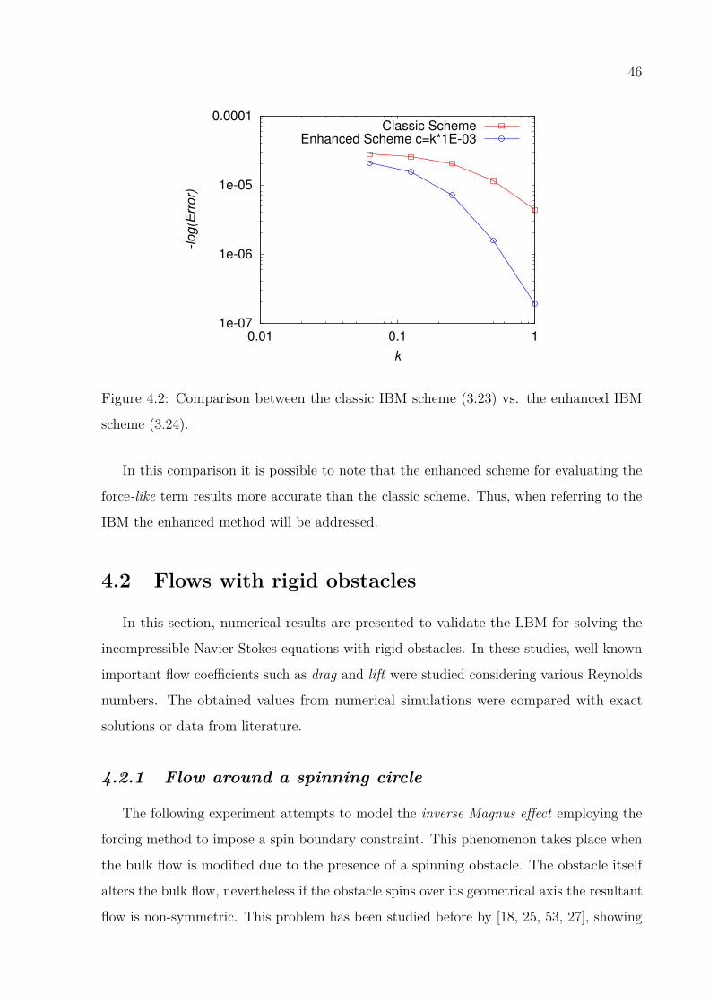
4.2 Comparison between the classic IBM scheme (3.23) vs. the enhanced IBM

scheme (3.24). . . . . . . . . . . . . . . . . . . . . . . . . . . . . . . . . . . 46

4.3 Flow patterns analysis considering RE = 20. The contour maps corresponds

to the distribution of the γ(r, t) vector field. . . . . . . . . . . . . . . . . 47

4.4 Drag and lift forces for different Reynolds numbers. . . . . . . . . . . . . . 48

4.5 Geometry of the flow around a cylinder, the geometry was re-scaled to

Lattice units. . . . . . . . . . . . . . . . . . . . . . . . . . . . . . . . . . . 48

4.6 Available solutions handed out for Test case 2D-1 (steady), the solutions

highlighted in red corresponds to the research group that employed a LBM-

BGK CFD solver. Adapted from [59]. . . . . . . . . . . . . . . . . . . . . . 50

4.7 Forcing method vs IBM, drag and lift analysis. . . . . . . . . . . . . . . . . 51

4.8 Velocity contour maps comparison. (a) forcing method and (b) IBM. . . . 52

4.9 Geometry of the flow around a cylinder. . . . . . . . . . . . . . . . . . . . 53

4.10 Flow around a circular cylinder: Velocity field considering different Reynolds

numbers. . . . . . . . . . . . . . . . . . . . . . . . . . . . . . . . . . . . . . 54

4.11 Drag coefficients at different Reynolds numbers. . . . . . . . . . . . . . . . 55

4.12 Geometry of the flow around a cylinder. . . . . . . . . . . . . . . . . . . . 55

4.13 Vortex principal separation modes. Adapted from [61]. . . . . . . . . . . . 56

4.14 Velocity field. . . . . . . . . . . . . . . . . . . . . . . . . . . . . . . . . . . 57

4.15 ux field variations during the simulations. . . . . . . . . . . . . . . . . . . . 58

4.16 uy field variations during the simulations. . . . . . . . . . . . . . . . . . . . 58

4.17 Density variations during the simulations. . . . . . . . . . . . . . . . . . . 59

4.18 Geometry of the flow around a square cylinder. . . . . . . . . . . . . . . . 59

4.19 Drag coefficients at different Reynolds numbers. . . . . . . . . . . . . . . . 60

4.20 Velocity field for the case with Reynolds 50. . . . . . . . . . . . . . . . . . 60

4.21 Geometry of the flow around a planar shield. . . . . . . . . . . . . . . . . . 61

4.22 Velocity field for different Reynolds numbers. . . . . . . . . . . . . . . . . . 62

List of Tables

3.1 IBM coefficients used in this work. . . . . . . . . . . . . . . . . . . . . . . 42

3.2 Equilibrium distribution optimal coefficients to ensure stability. . . . . . . 42

4.1 History convergence for Kovasznay Flow. . . . . . . . . . . . . . . . . . . . 45

List of Symbols

u , v Scalar functionsu ,v Vectorial functionsnd Number of spatial dimensions, (in this work fixed in 2)Hm Hilbert vectorial space regular enough till the m derivative(·; ·) Inner product〈·; ·〉 Dual-like productΩ Lipschitz domain∂Ω,Γ Regular enough boundariesLin(·, ·) Space of linear mapsKin U Kinematic admissible manifoldVar U Kinematic admissible vectorial spaceT,D, I Second order tensors(·)∗ Adjoint quantity of the vector, set (·)(·)T Transpose quantity of the vector, tensor (·)(·) Admissible variation of the vector, set (·)∇(·) Gradient of the scalar, vectorial field (·)div(·) Divergent of the vectorial field (·)(·), (·) First and second time derivative of the scalar, vectorial field (·),

respectively

15

1 INTRODUCTION

1.1 Motivation

Coupled problems like Fluid-Structure Interaction (FSI) are of special interest in many

engineering areas. The flow bounded by solid structures is possible to be solved knowing

the shape and position of the solid domain; as a consequence of this interaction the fluid

exerts on the solid reactive forces. In this context it is important to understand:

a) the magnitude of the forces that the fluid exerts on the solid domain;

b) the nature of those forces: are they transient or instantaneous or quasi-static?

c) and, finally: how the solid domain behaves in presence of fluid forces?

It is important to understand the nature of the forces that the fluid prints over the solid

domain, to describe common effects like aircraft’s fluttering, sock’s flapping, airbag’s

inflation, blood flow and arterial dynamics, among others. Basically the equilibrium of

forces between solid and fluid domains can be characterized in three ways: (i) unstable,

(ii) quasi-stable and (iii) stable. In this context a stable equilibrium corresponds to any

state of motion that remains constant during the motion. On the other hand, if the state

of motion addresses changes, in absence of forces, the equilibrium is no longer stable;

allowing to describe unstable and quasi-stable equilibriums.

Therefore, studies considering FSI phenomena are important to better understand

catastrophic events like the falling down of the Tacoma Narrows Bridge (see Figure 1.1);

or for the understanding on how to design efficient prosthetic devices such as stents for

biomedical engineering, as shown in Figure 1.2.

16

(a) Before collapse. (b) During collapse.

Figure 1.1: Tacoma Narrows bridge collapse

Figure 1.2: Stent function preventing stenosis, adapted from [14]

As reported by Maugin [33, 34, 35] over the last centuries there has been a compelling

need to reproduce the complex behavior of nature with coupled phenomena. In this

context, the FSI problems experienced a remarkable evolution of knowledge employing

experimental analysis. Among the several analysis, we can highlight the wind tunnels that

are often used to evaluate the performance of a prototype when subjected to aerodynamics

forces, see Figure 1.3.

17

Figure 1.3: Adapted from Mercedes Benz [4].

The use of experimental techniques like analysis with a wind tunnel is helpful to

understand the behavior of a prototype. Nevertheless, the use of the wind tunnel does

not give hints for optimizing the prototype and also does not give information to forecast

the behavior of the prototype when subjected to different forces or scenarios. In some

cases, the experiment is difficult to characterize, because it is entangled to determine a

reliable technique to measure non-dimensional numbers like: Reynolds number1, Mach

number2, and Froude number3. As mentioned by Lönher [31] the accurate control of these

three number is often complicated, specially when considering events that involves the

destruction of the prototype or the wind tunnel itself or human casualties. For example

the development of (nuclear) bombs does not allows to use wind tunnels, back in the

1940’s and 1950’s nuclear tests where often used and considered necessary to validate new

designs and combination of gunpowder. At the present time computational mechanics

allows to understand the "satisfactory" combination of gunpowder and other materials to

provoke the destruction of a desired target, without detonating a single bomb.

The present challenges for computational mechanics concern topics like:

• the partial replacement of experimental analysis with numerical simulations,

• analyze the results coming from numerical simulation to forecast dependencies,

• reduce the cost of experiments to the minimum.1The Reynolds number is the ratio of inertial forces towards viscous forces.2The Mach number is the ratio of the velocity past an obstacle refereed to the velocity of sound.3The Froude number is the ratio of the flow inertia towards the external forces.

18

In this context the computational mechanics is presented as an alternative to fill-in the

gaps left by experimental analysis when modeling complex situations like: bio-medical

devices design like the one shown with Figure 1.2. Recently, computational mechanics has

provided answers towards the characterization of blood flow considering bifurcations, as

reported by Artoli et al. [2]. In [2] the flow faces changes on the domain, modifying the

distribution of the velocity vector field and the shear stresses. In particular, considering

computational Hemodynamics, the works of Artoli [1, 3] analyzes the possibilities to model

blood flow in domains reconstructed with Computational Tomography. Specially in [3], the

focus is put on studying the process of white blood cell margination. The margination of a

blood cell refers to the state of equilibrium of a cell immersed in the blood flow (The cell

can follow the blood stream and roll). These analysis allow to understand several process

like immunity decay towards the presence of infections. Inflammation of an infected area is

the result of white blood cell’s margination, coming from the blood vessel and infiltrating

in to the damaged tissue.

1.2 Objectives and contributions of the work

The main contribution of this work is to establish a methodology to simulate

incompressible flows considering the inclusion of arbitrary-shaped obstacles. For this

we present a self-consistent technique to obtain the Euler-Lagrange equations. And

afterwards solve them employing the Lattice Boltzmann Methods coupled to the Immersed

Boundary Method. To determine the robustness of the methodology we show several

simulations highlighting the agreement between the reference’s gold standards and our

results.

1.2.1 Methodology to model FSI: Euler-Lagrange equations

In order to model the behavior of fluid flow considering complex conditions, in this

section some important continuum mechanics concepts are presented. The procedure

to formulate the problem is the result of: (i) kinematic admissibility, (ii) mathematical

duality and, (iii) the Principle of Virtual Power Balance (PVPB).

This modeling technique has been applied showing the equivalence between the PVPB

and the Euler-Lagrange equations corresponding to coupled problems in the works of [12,

19

20, 32], concerning physics like: solid mechanics, fluid mechanics, electro-magnetics,

dissipative mechanics, among others. Thus, the PVPB has been used as an alternative

method to model coupled physics. The validity of this method was analyzed in [21, 36]

highlighting the modeling of complex physics. Moreover, the Constitutive modeling has

used the PVPB approach to characterize the kinematic compatible loadings (external and

internal loadings) [17, 48, 43].

1.2.2 Numerical solutions: LBM-IBM

Once the Euler-Lagrange equations governing the complex fluid flow are derived, a

numerical method has to be applied in order to obtain approximate solutions. To this, we

employ the Lattice Boltzmann Method (LBM) due to the successfully to obtain accurate

solutions for the incompressible Navier-Stokes equations [11, 24, 40]. The method is very

attractive from the computational point of view and when combined with other methods

offers an interesting approach for FSI problems, as will be shown.

To solve realistic problems like the inclusion of arbitrary-shaped obstacles in the flow we

couple LBM with the IBM. The IBM is a computational option to refine the grid in order

to achieve an accurate representation of complex geometries, that can be viewed in works

of Peskin [44, 45, 47, 37, 46]. However, in this work a different scheme for dealing with

rigid obstacles is discussed, validated and compared with classical approach by available

benchmarks in the literature.

1.3 Dissertation’s structure

This work is organized as follows: a methodology for obtaining the Euler-Lagrange

equations that models obstructed fluid flow is shown in chapter 2. In chapter 3,

the numerical methodologies are presented and analyzed to obtain the solution of

the corresponding boundary value problem, featuring methods like LBM and IBM.

A combination of these numerical techniques are validated and tested in chapter 4,

demonstrating the versatility and robustness of the computational implementation. Finally,

future works, conclusion and remarks are adressed in chapter 5.

20

2 CONTINUUM MECHANICS

MODELING FRAMEWORK

This chapter presents a methodology to study functional dependencies between

generalized loadings (stresses, body forces, surface tractions) and generalized displacements

(displacements, velocities, strain rates). The Euler-Lagrange equations are responsible for

characterizing kinematic compatible loadings with the adopted kinematics. In this work

the Euler-Lagrange equations are obtained following the three invariant steps:

i) define convenient kinematics. The kinematics is defined characterizing the regularity

and the appropriate boundary restrictions to model the problem;

ii) define dual-like power measures. The dual-like measures represents the power

expended to perform changes on the kinematic state variables; and

iii) evoke the PVPB, to characterize the equilibrium.

The consequences of this procedure are equivalent to consider the balance of momentum

as reported by Truesdell [56, 58, 55] and Germain [21]. For example, if needed to evaluate

the weight of an object, firstly it is required to provide a vertical displacement degree of

freedom, acknowledging a rigid motion. Secondly, it is necessary to measure the exerted

virtual power. Finally the expression of the virtual power balance resumes the fact that

the density of the object times gravity is the weight of the object.

For the scope of continuum mechanics the virtual power balance has been analyzed

in the following works [5, 6, 42, 54]. For certain cases like linear elasticity, creeping flow

mechanics, among others, the expressions obtained employing the PVPB are equivalent

to find the conditions that minimizes a particular cost functional, as can be viewed

in [15, 51, 41]

2.1 Notation

In this work, scalar fields are defined as u, v and bold symbols are used to denote

the vector fields u,v. Let Ω ⊂ Rnd, nd = 2, 3, be a bounded domain with a Lipschitz

21

boundary ∂Ω. In this domain we set

L2(Ω) ≡v ∈ Ω :

∫Ω|v|2 dΩ <∞

,

as the space of square integrable functions, and

H1(Ω) ≡v ∈ L2(Ω) : ∇v ∈ L2(Ω)

,

where ∇ denotes the gradient operator.

For vectorial fields the following generalization is valid:

L2(Ω) = (L2(Ω))nd ,

H1(Ω) = (H1(Ω))nd .

As reported by Taroco [54] and Berdichevsky [5, 6] for functional spaces, the inner

product is introduced as (u; v) = u · v. The Mathematical Duality is represented by

〈u; v〉U∗×U =⇒ (u; v), where u ∈ U∗ and v ∈ U , with the subset U∗ being the dual subset

of U .

2.2 Kinematics

For the purposes of this work a general description for a motion is done by defining

a mechanical state field denoted by E. Thus, for any x ∈ Ω, the generalized mechanical

state yields the following definition:

E : Ω→ Rnd,

x 7→ E. (2.1)

For the scope of this analysis, the first gradient modeling scheme is employed. The first

gradient models the balance between generalized forces and generalized stresses, this theory

is explained in the works of [5, 6, 54]. As a consequence of the first gradient scheme it is

necessary to define a generalized motion action D(E) as:

22

D : Lin(Rnd,Rnd),

E 7→ D(E) = ∇E, (2.2)

where Lin(Rnd,Rnd) represents the space of linear functions with support and range on

the vectorial space Rnd.

2.3 Motion Actions: Kinematic Constraints

The mechanical state functional space is characterized taking into account: well-posed

regularity, Dirichlet’s boundary conditions (often known as essential boundary conditions)

and if needed distributed constraints. For this analysis the mechanical state lies on the

following manifold:

Kin U = w ∈ H1(Ω) : w|∂ΩD= ED ,G(w) = 0 ∈ Ω, (2.3)

where ∂ΩD denotes the boundary with prescribed values for the mechanical state E, in this

case E−ED = 0 and G(w) = 0 represent a distributed restriction in Ω. It is also possible

to characterize the subspace Var U of kinematically admissible variations as follows:

Var U = u1 − u2 ∈ Var U : u1,u2 ∈ Kin U . (2.4)

2.4 Power Duality

The kinematic admissible manifold (2.3) takes into account measures of the mechanical

state and its gradient. In this context two different powers are recognized:

• Internal Power (P int). Addresses the expended power used to perform changes in the

strain rate tensor. The internal power is considered to be a linear and continuous

functional defined over the D(E), which can be mathematically expressed as

P int : Rnd∗ × Rnd → R,

23

where the space Rnd∗ is the dual space of Rnd. Using the Riesz representation

theorem [54], the linear operator has the unique representation,

P int(D(E)) = 〈A;D(E)〉Rnd∗×Rnd .

The new element A ∈ Lin(Rnd,Rnd) is called stress tensor.

• External Power (P ext). Addresses the expended power used to perform changes in

the mechanical state vector. The external power is considered to be a linear and

continuous functional defined over the mechanical state, which can be mathematically

expressed as

P ext : Rnd∗ × Rnd → R.

Using Riesz representation theorem, the linear operator has unique representation,

P ext(E) = 〈f ; E〉Rnd∗×Rnd ,

where f ∈ Rnd∗ represents a generalized external load.

These duality products must satisfy the following properties [54]:

〈A;D(E)〉Rnd∗×Rnd = 0, ∀D(E) ∈ Rnd ⇒ A = 0,

〈A;D(E)〉Rnd∗×Rnd = 0, ∀A ∈ Rnd∗ ⇒ D(E) = 0,

〈f ; E〉Rnd∗×Rnd = 0, ∀E ∈ Rnd ⇒ f = 0,

〈f ; E〉Rnd∗×Rnd = 0, ∀f ∈ Rnd∗ ⇒ E = 0.

2.5 Virtual Power Balance in Continuum Mechanics

To model continuum mechanics problems in this work the balance of virtual power

is used, which is equivalent to model the problem considering the balance of momentum

balance of mass and other constraints, as reported by Germain [20, 21]. To use the virtual

power balance the following axiom is stated:

Axiom 2.1 (Principle of Virtual Power Balance (PVPB)). Let a system Ω be in equilibrium

24

with respect to a given frame of reference; then, in any virtual motion, the virtual power

of all the internal forces and external forces acting on Ω is null, i.e.:

P int(D(E)) + P ext(E) =⟨A;D(E)

⟩Rnd∗×Rnd

+⟨f ; E

⟩Rnd∗×Rnd

= 0 ∀ E ∈ Var U . (2.5)

The PVPB itself retrieves a mathematical expression for the concept of equilibrium

which is used to characterize the kinematic compatible loadings A(E) ∈ Rnd∗ and f ∈

Rnd∗. For this objective, the adjoint transformation results particularly useful for this

characterization, as mentioned in [41, 54]. Thus, the inner power functional can be

rewritten employing the adjoint transformation as follows:

⟨A;D(E)

⟩Rnd∗×Rnd

=⟨D∗A; E

⟩Rnd∗×Rnd

.

where D∗ denotes the adjoint operator for the linear mapping D. As a consequence of this

adjoint transformation, the external kinematic compatible loading f ∈ Rnd∗ belongs to the

same space as the adjoint operator applied to the stress tensor D∗A. The adjoint operator

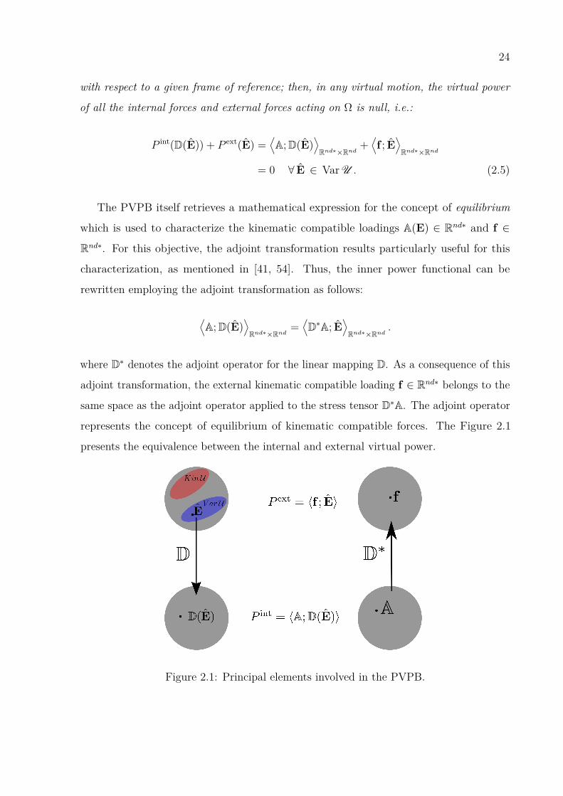
represents the concept of equilibrium of kinematic compatible forces. The Figure 2.1

presents the equivalence between the internal and external virtual power.

Figure 2.1: Principal elements involved in the PVPB.

25

2.6 Unconstrained mechanical state manifolds

problem

The mechanical state was defined over a manifold that contains restrictions due to the

essential boundary conditions and distributed constraints. As shown by [5, 6, 54], it is

possible to remove from the adopted manifold (2.3) restrictions like: essential boundary

conditions and/or distributed constraints. In these analysis, the distributed boundary

constraint, G(w) = 0 ∈ Ω is removed from the manifold resulting in:

Kin U λ = w ∈ H1(Ω) : w|∂ΩD= ED. (2.6)

Accounting admissible mechanical state’s variations, the following subspace is defined:

Var U λ = u1 − u2 ∈ Var U λ : u1,u2 ∈ Kin U λ . (2.7)

The physical problems remains invariant, but the kinematics addressed changes. In

order to model the same problem with different kinematic settings, the expression of

the PVPB must be updated. In this context, a new kinematic compatible loading λ

is introduced over a particular functional space Λ. The functional space Λ has enough

regularity to maintain the problem well-posed. In this case λ plays the role of a Lagrange’s

multiplier, see [9, 15, 51] for more details. The changes in the PVPB yields the following

problem:

Problem 2.1 (Unconstrained mechanical state manifolds problem). Given a source loading

function f ∈ Rnd∗, find the pair (E, λ) ∈ Kin U λ× Λ, such that for all (E, λ) ∈ Var U λ× Λ

P int(D(E)) + P ext(E) =⟨A;D(E)

⟩Rnd∗×Rnd

+⟨f ; E

⟩Rnd∗×Rnd

+(λ;G(E)

)+(λ;G(E)

)= 0. (2.8)

Once again the adjoint transformation of the linear maps D and G are useful for

characterizing the functional dependencies between the kinematic compatible loadings

(A ∈ Rnd∗, f ∈ Rnd∗, λ ∈ Λ) and the mechanical state variables (E,D(E)).

The use of Lagrange multipliers grants the imposition of boundary constraints or

distributed restrictions allowing to build up more flexible kinematic admissible manifolds.

26

In fluid mechanics for example, the use of Lagrange multipliers allows to remove the free

divergence restriction from the kinematic admissible manifold to simulate incompressible

flows.

2.7 Fluid Mechanics Variational Framework

In this section, based on the three steps modeling procedure, the incompressible Navier-

Stokes equations are obtained. The mechanical state is defined in terms of the velocity

vector field and the strain rate tensor field, consistently with the first gradient theory,

where two different measures of expended power are recognized: internal and external.

Thus, the characterization of kinematic compatible loadings is done with the postulation

of the PVPB, where the free divergence constraint and fluid-solid interface restriction are

weakly enforced by Lagrange multipliers.

2.7.1 Fluid mechanics mechanical state

To start the development some definitions are introduced. The velocity vector field is

given by:

u : Ω× [0, T ]→ Rnd,

(x, t) 7→ u, (2.9)

where x represents any arbitrary point of the domain Ω ∈ Rnd and t represents an arbitrary

time instant of the temporal interval [0, T ]. The strain rate tensor is introduced as:

D : Lin(Rnd,Rnd),

u 7→ D(u) = ∇u. (2.10)

Finally for this problem the mechanical state is well-posed by defining the manifold where

the velocity vector field lies on:

Kin U = w ∈ H1(Ω), essential boundary conditions.

27

The kinematic admissible variations of the mechanical state reside on the following vectorial

subspace:

Var U = u1 − u2 ∈ Var U : u1,u2 ∈ Kin U .

2.7.2 Fluid mechanics measures of expended power

The fluid mechanics mechanical state description concluded with the definition of

admissible kinematics written in terms of a velocity vector field and a strain rate tensor.

As a consequence of this description two measures of expended power can be defined. In

one hand the internal power can be written as:

P int(D(u)) = 〈Tf ;∇u〉Rnd∗×Rnd ;

The new element Tf ∈ Lin(Rnd,Rnd) is called stress tensor. On the other hand, the

external power can be written as:

P ext(u) = 〈(f + ρu · ∇u + ρ u); u〉Rnd∗×Rnd ,

where f ∈ Rnd∗ represents a kinematic compatible external load, ρu ·∇u ∈ Rnd∗ represents

the effects of convective forces and ρ u ∈ Rnd∗ represents the inertial kinematic compatible

loads.

2.7.3 Fluid mechanics Virtual Power Balance

Here, the free divergence and the fluid-solid interface constraints are weakly imposed by

a Lagrange multiplier. The Lagrange multiplier associated to the divergence free presents

the physical behavior of the hydrostatic pressure p ∈ L2(Ω) and the effects of the fluid-solid

interface are taken into account considering a Lagrange multiplier γ ∈ L2(Γ) that enforces

the boundary constraint u− usl = 0 on Γ.

Problem 2.2 (Incompressible Navier-Stokes equations in presence of a regular obstacle).

Given a source loading function f ∈ Rnd∗, for each t ∈ [0, T ] find the triple (u, p,γ) ∈

28

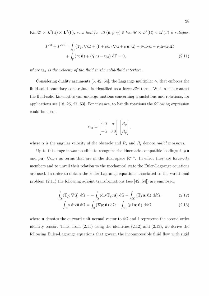
Kin U × L2(Ω)× L2(Γ), such that for all (u, p, γ) ∈ Var U × L2(Ω)× L2(Γ) it satisfies:

P int + P ext =∫

Ω(Tf ;∇u) + (f + ρu · ∇u + ρ u; u)− p divu− p divu dΩ

+∫

Γ(γ; u) + (γ; u− usl) dΓ = 0, (2.11)

where usl is the velocity of the fluid in the solid-fluid interface.

Considering duality arguments [5, 42, 54], the Lagrange multiplier γ, that enforces the

fluid-solid boundary constraints, is identified as a force-like term. Within this context

the fluid-solid kinematics can undergo motions concerning translations and rotations, for

applications see [18, 25, 27, 53]. For instance, to handle rotations the following expression

could be used:

usl =

0.0 α

−α 0.0

Rx

Ry

,where α is the angular velocity of the obstacle and Rx and Ry denote radial measures.

Up to this stage it was possible to recognize the kinematic compatible loadings f , ρ u

and ρu · ∇u,γ as terms that are in the dual space Rnd∗. In effect they are force-like

members and to unveil their relation to the mechanical state the Euler-Lagrange equations

are used. In order to obtain the Euler-Lagrange equations associated to the variational

problem (2.11) the following adjoint transformations (see [42, 54]) are employed:

∫Ω

(Tf ;∇u) dΩ = −∫

Ω(divTf ; u) dΩ +

∫∂Ω

(Tfn; u) d∂Ω, (2.12)∫Ωp divu dΩ =

∫Ω

(∇p; u) dΩ−∫∂Ω

(p In; u) d∂Ω, (2.13)

where n denotes the outward unit normal vector to ∂Ω and I represents the second order

identity tensor. Thus, from (2.11) using the identities (2.12) and (2.13), we derive the

following Euler-Lagrange equations that govern the incompressible fluid flow with rigid

29

obstacles:

ρ u + ρu · ∇u− divTf + f +∇p = 0, in Ω,

divu = 0, in Ω,

(Tf − p I) n = 0, on ∂ΩN ,

(Tf − p I) n = γ, on Γ,

u− usl = 0, on Γ,

Essential boundary conditions for: u.

(2.14)

The system (2.14) characterizes the force-like members f , ρ u, ρu · ∇u and ∇p as

body forces. Furthermore, the Lagrange multiplier that enforces the fluid-solid boundary

constraint γ shares the same properties as a surface traction vector. It is also possible to

note the homogeneous Neumann’s boundary conditions, the Dirichlet boundary conditions,

the free divergence constraint and the fluid-solid interface constraint. To give closure to

the previous problem, the characterization of the internal kinematic compatible loading

Tf is presented. In this case isotropic and Newtonian behavior is assumed yielding the

following expression:

Tf = µ ∇u,

where µ represents the viscosity of the fluid.

The Euler-Lagrange equations (2.14) allows to model the incompressible Navier-Stokes

equations considering the inclusion of obstacles to alter the flow. In the next chapter

these equations will be discretized by the Lattice Boltzmann Method and, in order to

tackle the presence of arbitrary shaped obstacles, two different techniques will be used:

the Forcing Method and the Immersed Boundary Method. While the Lattice Boltzmann

Method is a technique capable of solving incompressible flows, the inclusion of arbitrary

shaped obstacles will be treated "efficiently" employing the Immersed Boundary Method.

30

3 NUMERICAL METHODS

In this chapter the numerical methods for solving the incompressible Navier-Stokes

equations (2.14) and the numerical techniques for dealing with fluid flow around rigid

obstacles are presented.

3.1 Introduction

The numerical methods used for solving fluid flow problems are part of a branch of

computational mechanics usually called as Computational Fluid Dynamics (CFD). In this

context, the Lattice Boltzmann method arises as an alternative to traditional solvers based

on the Finite Volume Method (FVM) or Finite Element Method (FEM) that considers

a discretized version of the Navier-Stokes equations as the starting point. The LBM

describes the kinetics of distribution of particles at the mesoscale. Formally, it can be

derived from the Lattice-gas cellular automata’s or from a specific discretization scheme of

the Boltzmann equation. In the last years the LBM has been successfully applied to study

the fluid flow in different applications such as in biomedical engineering [22], heat transfer

problems with phase change [60] and also turbulent flows [19].

Traditional numerical methods, such as the FEM, when employed to approximate the

Navier-Stokes equations are often challenged by the convective non-linear term, which

requires a methodology to linearize the system of equations. Moreover, the problem is

commonly approximated in the mixed form, which demands additional computational

operations. Other numerical challenge is ensure the free divergence for this problem.

In this context, the LBM overcome all these difficulties, because this method naturally

treat the non-linear term and does not need to solve the mixed problem to enforce the

incompressibility [40, 29] due to the explicit nature of the method, moreover is simple

to implement and due to its high locality an efficient parallel implementation can be

exploited [10].

To simulate the fluid flow including rigid obstacles using the Lattice Boltzmann Method

we employ the Forcing Method [26] and the Immersed Boundary Method [40, 46, 29] to

represent the boundary domain conditions and fluid/obstacle interface conditions.

31

3.2 Lattice Boltzmann Method (LBM)

Here the classical Lattice Boltzmann method for fluid flow is described considering an

incompressible fluid. The appropriate treatment of boundary conditions and obstacles are

considered within the traditional LBM scheme.

3.2.1 Boltzmann’s Equation

Based on the kinetic theory of gases it is possible to show that any changes in the

state of pressure, temperature and volume are consequences to the lack of equilibrium

between the molecules that interact in the gas. Every molecule in the gas interact with

other particles continuously colliding achieving a random motion. As reported in [57] for

describing this theory the following assumptions are taken into account:

• the density of a group of molecules might change due to random collisions between

other particles; and

• the density of a group of molecules might change due to volumetric forces.

Given a set of particles, in a fixed time t, the particles inside the spatial range r + δr whose

velocity rank is bounded by c + δc can be measured with the probability distribution

function f(r, t). Neglecting external forces, the kinetic theory of gases establishes the

following conservation law known as the Boltzmann’s equation:

∂f

∂t+∇f · c = Q(f); (3.1)

where Q(f) is the collision operator, which measures the deviation from equilibrium of

the particles. In one hand if Q(f) = 0 the molecules have achieved equilibrium, whereas

on the other hand if Q(f) 6= 0 it means that the particles have not achieved a state of

equilibrium.

The collision operator defined by Bhatnagar–Gross–Krook (BGK) [7], yields the

following expression:

Q(f) = ω (f eq − f(r, c, t)) ; (3.2)

where ω represents the frequency of collisions between the particles and f eq(r, c, t) is the

so called equilibrium probability distribution. Equations (3.1) and (3.2) when combined

32

results in the Boltzmann’s equation with the BGK-operator, which is given by

∂f

∂t+∇f · c = ω (f eq − f) . (3.3)

The previous expression forms the basis for the Lattice Boltzmann Method that will

be described shortly next. The LBM with the BGK collision operator can be shown to

recover the macroscopic behavior of the incompressible Navier-Stokes equations for fluid

flow, as shown in [11].

3.2.2 LBM

In order to obtain the expression of the LBM to perform numerical simulations the

Boltzmann equation with the BGK-operator (see equation (3.3)) is spanned considering

i = 0, · · · , l directions. In this work the spanned directions corresponds to the scheme

proposed by He and Luo [24] and also discussed in Mohamad [40]. As a consequence, the

following expression is written as:

∂fi∂t

+∇fi · ci = ω (f eqi − fi) . (3.4)

In this case the regularity of the interest field fi grants the possibility to replace the

continuous operators (time derivative and spatial gradient) with finite difference schemes

for time and space;

∂fi∂t' fi(r, t+ δ t)− fi(r, t)

δ t, (3.5)

∇fi · ci 'fi(r + δ ri, t+ δ t)− fi(r, t+ δ t)

‖δ ri‖δ ri‖δ ri‖

· ci, (3.6)

where ‖δ ri‖ = (δ ri; δ ri)1/2. Replacing (3.5) and (3.6) in the Boltzmann’s equation (3.4)

we obtain the next equivalence:

fi(r, t+ δ t)− fi(r, t)δ t

+ fi(r + δ ri, t+ δ t)− fi(r, t+ δ t)‖δ ri‖

δ ri‖δ ri‖

· ci = ω (f eqi − fi) .

(3.7)

33

Considering ci = δ ri/δ t the previous expressions results in the LBM

fi(r + δ ri, t+ δ t)− fi(r, t)δ t

= ω (f eqi − fi) ,

→ fi(r + δ ri, t+ δ t) = fi(r, t) + δ t ω (f eqi − fi) . (3.8)

The product δ t ω defines a new variable τ−1 which is known as relaxation parameter.

Bearing on numerical methods equation (3.8) is linear, explicit and has great deal of local

operations, which allows to perform rapid computations. The relaxation parameter must

satisfy the following relation:

µ = (δr; δr)3 δt (τ − 0.5), (3.9)

where τ must be greater than 0.5 in order to avoid a fluid with negative viscosity. Lower

values of τ represents fluids with a viscosity µ near zero. These fluids will achieve the

equilibrium state faster than more viscous fluids.

3.2.3 Equilibrium Distribution

The equilibrium distribution characterizes the steady state of the probability

distribution function f(r, t). For particles moving in a macroscopic framework with

velocity u, the normalized Maxwell-Boltzmann distribution can be written as follows:

fMB = 3 ρ2 π exp

[−3

2(c− u)2], (3.10)

where ρ represents the macroscopic density of the fluid. To complete the problem of

computing the equation (3.8), the equilibrium distribution is defined when applying a

second order asymptotic expansion of the Maxwell-Boltzmann distribution, which yields

the following expression:

f eq = φ(ρ)(A+B (c; u) + C (u; u) +D (c; u)2

), (3.11)

where A,B,C,D ∈ R and φ(ρ) : R→ R that will be defined next.

34

3.2.4 The D2Q9 Lattice array

In this work, we adopt a D2Q9 Lattice array (two dimension with nine velocity

directions) proposed by He and Luo [24] to perform all simulations. In this context, we can

evaluate the A,B,C and D coefficients where the equations (3.8) and (3.11) are restrict

to this scheme. Thus, in a Cartesian frame of reference the D2Q9 model is given by:

c0 = (0, 0),

c1 = (1, 0) c2 = (0, 1) c3 = (−1, 0) c4 = (0,−1),

c5 = (1, 1) c6 = (−1, 1) c7 = (−1,−1) c8 = (1,−1).

(3.12)

These velocity directions are described in Figure 3.1.

Figure 3.1: The D2Q9 Lattice array.

In the D2Q9 Lattice model it is possible to find particles: at rest (f0), moving in

horizontal and vertical directions (f1 − f4), and moving in diagonal directions (f5 − f8).

The equilibrium distribution when considering the D2Q9 Lattice model is given by the

following expression:

f eqi (c, t) = wi

ρ + ρ0

1 + 3 (v ci; u)v2 − 3

2(u; u)v2 + 9

2

((v ci; u)v2

)2, (3.13)

where v = ‖δr‖ (δ t)−1 is the Lattice grid velocity and the weighting directions represented

35

by wi are shown next

w0 = 49 ,

w1 = w2 = w3 = w4 = 19 ,

w5 = w6 = w7 = w8 = 136 .

It is important to remark that Chen and Doolen [11] showed that the LBM equation (3.8)

with the equilibrium distribution (3.13) recovers the macroscopic behavior of the

incompressible Navier-Stokes equations. It is also shown that the LBM is a second

order accurate scheme in both time and space. In this work, the equilibrium distribution

previously described in general terms with the coefficients A,B,C and D was adapted to

ensure improved numerical stability. To this end the guidelines proposed in the research

works of Golbert et al. [22] and Chen and Doolen [11] were employed.

In order to perform numerical simulations employing the LBM the following work-flow

is used:

1) Initialization: here the probability distribution functions fi(r, t) are initialized;

2) Collision: the probability distributions are altered accounting the BGK operator,

see the right hand side of equation (3.8);

3) Streaming: the probability distributions are streamed to the neighboring nodes

following the left hand side of equation (3.8).

After the computations of equation (3.8) with the D2Q9 Lattice model, the macroscopic

fluid density ρ and the macroscopic momentum are evaluated using the following equations:

ρ =8∑i=0

fi,

ρu =8∑i=0

fi ci.

3.2.5 Boundary Conditions

The LBM represented by equation (3.8) recovers the macroscopic behavior of the

incompressible Navier-Stokes equations. In the context of the LBM, the boundary

conditions like no-slip and/or essential boundary conditions must be treated properly.

36

Several methods for treating boundary conditions within the LBM have been described

in [29, 40]. Periodic boundary conditions are used only when the flow solution is periodic;

consequently, periodic boundary conditions conserve mass and momentum at all times.

In the bounce-back scheme the probability distributions fi that hit a rigid wall during

the propagation are reflected back considering the incoming direction. The bounce-back

scheme is usually applied to impose a no-slip boundary condition. The forcing method

applies instantaneous impulses the interface nodes to comply the boundary constraint.

This scheme was proposed by Mohamad and Kuzmin [39] and will be detailed next in

order to be applied for boundary conditions at rigid obstacles. In order to obtain accurate

solutions for the flow around rigid obstacles, with low computational cost the Immersed

Boundary Method is presented. Two frames of references are presented in one hand the

Eulerian Lattice grid where the fluid is solved. And on the other hand, a Lagrangian set

of nodes where the fluid-solid interface is defined.

3.3 Fluid-structure interaction

Here the two techniques used to treat fluid-structure interaction with rigid and moving

obstacles within the LBM solver are presented: the forcing method and the Immersed

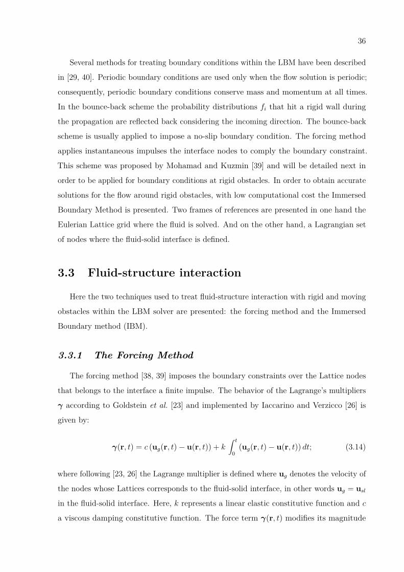
Boundary method (IBM).

3.3.1 The Forcing Method

The forcing method [38, 39] imposes the boundary constraints over the Lattice nodes

that belongs to the interface a finite impulse. The behavior of the Lagrange’s multipliers

γ according to Goldstein et al. [23] and implemented by Iaccarino and Verzicco [26] is

given by:

γ(r, t) = c (ug(r, t)− u(r, t)) + k∫ t

0(ug(r, t)− u(r, t)) dt; (3.14)

where following [23, 26] the Lagrange multiplier is defined where ug denotes the velocity of

the nodes whose Lattices corresponds to the fluid-solid interface, in other words ug = uslin the fluid-solid interface. Here, k represents a linear elastic constitutive function and c

a viscous damping constitutive function. The force term γ(r, t) modifies its magnitude

37

trailing the discrepancies between a known data-set ug and a present data-set u. This

technique was applied in the work of [38] for evaluating the drag and lift forces of a flow

considering circular obstacles. Specifically, within the LBM this force field is computed as:

γ(r, t) = c (ug(r, t)− u(r, t)) + k∑n

(ug(r, ti)− u(r, ti)) δ tn. (3.15)

Then finite impulses are applied to the LBM equation in order to impose the proper

boundary condition. The forcing term is applied in each Lattice direction i as [39]:

Si = δt

v(ci; γ) . (3.16)

Thus the forcing term imposes over the corresponding Lattices a finite impulse given by:

8∑i=0

vSi(r, t) ci =8∑i=0

δt (ci; γ) ci

=8∑i=0

δt (ci; ci) γ = δtγ (3.17)

and then the LBM equation (3.8) is modified to include this forcing term as:

fi(r + ci δt, t+ δt) = fi(r, t) + 1τ

(f eqi − fi(r, t)) + wi Si(r, t), (3.18)

Within this context, it is important to note that the kinematic compatible sources Si(r, t)

do not alters the balance of the mass, that is

8∑i=0

wi Si(r, t) = 0.

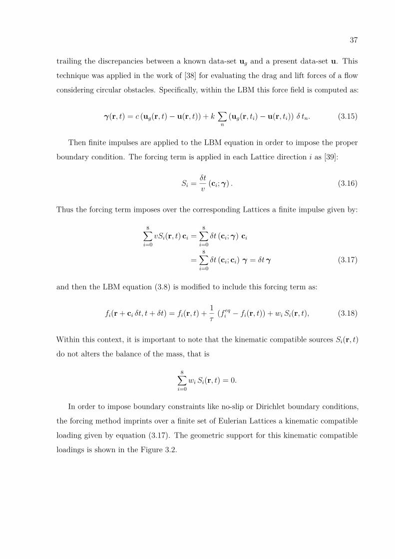
In order to impose boundary constraints like no-slip or Dirichlet boundary conditions,

the forcing method imprints over a finite set of Eulerian Lattices a kinematic compatible

loading given by equation (3.17). The geometric support for this kinematic compatible

loadings is shown in the Figure 3.2.

38

Figure 3.2: Physical situation (left) and forcing method approach (right), the affected

Lattices are highlighted in blue.

3.3.2 Immersed Boundary Method

Other alternative to treat the inclusion of arbitrary shaped obstacles is the Immersed

Boundary Method. The IBM gives support to the fluid-solid interface considering a

Lagrangian set of nodes also known as Lagrangian markers. Hence two frames of references

are considered: the flow defined over an Eulerian grid and the fluid-solid interface defined

over a finite set of Lagrangian nodes.

When using the classical LBM and the bounce-back scheme or the forcing method of

Mohamad [39] for handling boundary conditions around rigid obstacles, some complexity

arises since they can have arbitrary and complex geometry, be moving in space or even

deformable. If the geometry of the obstacle is complex a staircase approximation such

as the one shown in Figure 3.2 would result; if the boundaries are deformable additional

constitutive equations have to be considered with the bounce back or a scheme like the

forcing method of Mohamad [39], which be very tricky to handle. Therefore, in all these

cases the classical LBM is not appropriate and its aforementioned advantages are lost.

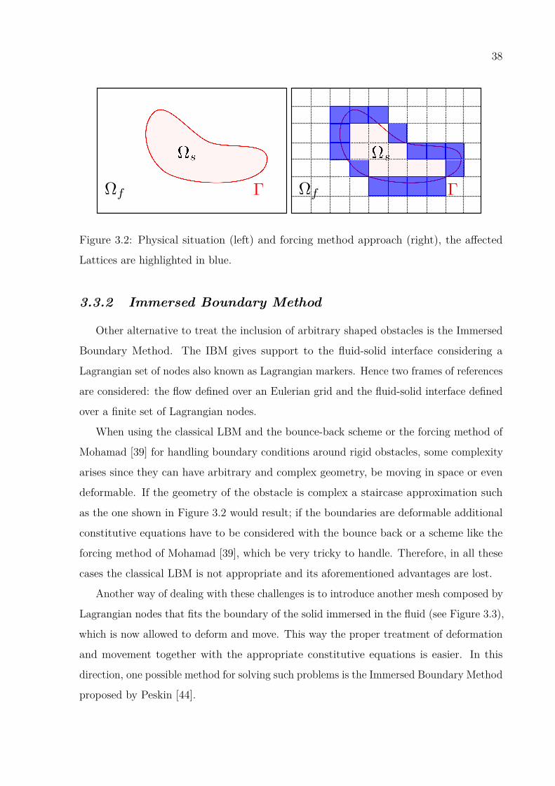
Another way of dealing with these challenges is to introduce another mesh composed by

Lagrangian nodes that fits the boundary of the solid immersed in the fluid (see Figure 3.3),

which is now allowed to deform and move. This way the proper treatment of deformation

and movement together with the appropriate constitutive equations is easier. In this

direction, one possible method for solving such problems is the Immersed Boundary Method

proposed by Peskin [44].

39

Figure 3.3: Physical situation (left) and IBM approach (right) with Lagrangian nodes

highlighted in red.

In FSI analysis the fluid-solid interface might not always agree with the Eulerian fluid

description, specially when one considers a complex geometry for the fluid-solid interface.

Figure 3.3 shows an example of fluid-solid interface with a complex geometry. A common

approach in these cases is to use a very refined grid for representing the complex interface,

however it induces a high computational cost. In this context, the IBM Boundary Method

arises as a viable option. The IBM represents a modeling technique to include the effects

of non-regular interfaces embedded in an Eulerian Lattice grid. In the work of Peskin [46],

the IBM uses interpolation schemes for the forces exerted by the solid to the fluid and

vice-versa to incorporate the appropriate boundary conditions.

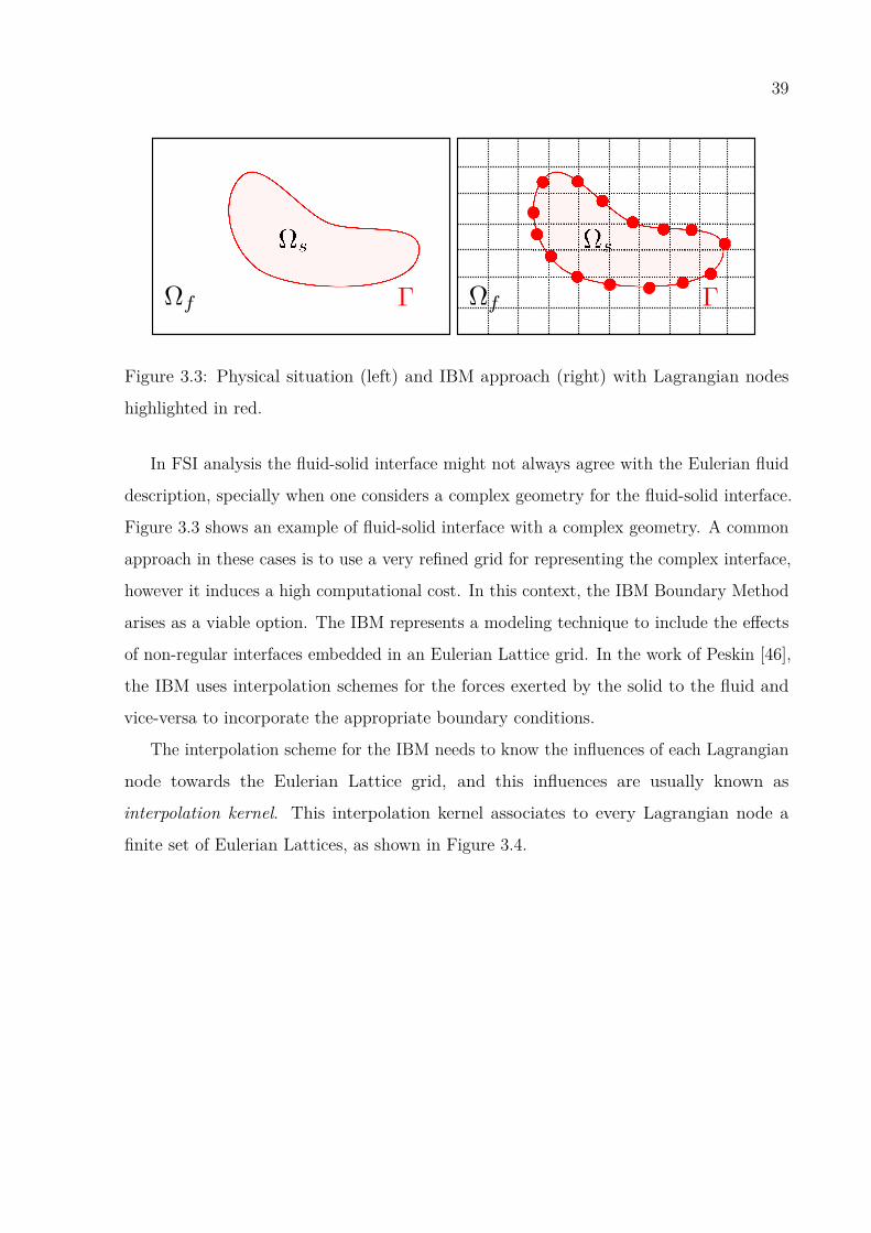
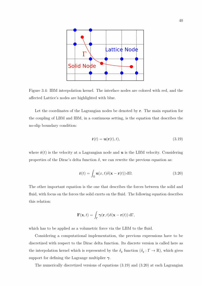
The interpolation scheme for the IBM needs to know the influences of each Lagrangian

node towards the Eulerian Lattice grid, and this influences are usually known as

interpolation kernel. This interpolation kernel associates to every Lagrangian node a

finite set of Eulerian Lattices, as shown in Figure 3.4.

40

Lattice Node

Solid Node

Figure 3.4: IBM interpolation kernel. The interface nodes are colored with red, and the

affected Lattice’s nodes are highlighted with blue.

Let the coordinates of the Lagrangian nodes be denoted by r. The main equation for

the coupling of LBM and IBM, in a continuous setting, is the equation that describes the

no-slip boundary condition:

r(t) = u(r(t), t), (3.19)

where r(t) is the velocity at a Lagrangian node and u is the LBM velocity. Considering

properties of the Dirac’s delta function δ, we can rewrite the previous equation as:

r(t) =∫

Ωu(x, t)δ(x− r(t)) dΩ. (3.20)

The other important equation is the one that describes the forces between the solid and

fluid, with focus on the forces the solid exerts on the fluid. The following equation describes

this relation:

F(x, t) =∫

Γγ(r, t)δ(x− r(t)) dΓ,

which has to be applied as a volumetric force via the LBM to the fluid.

Considering a computational implementation, the previous expressions have to be

discretized with respect to the Dirac delta function. Its discrete version is called here as

the interpolation kernel which is represented by the δg function (δg : Γ→ R), which gives

support for defining the Lagrange multiplier γ.

The numerically discretized versions of equations (3.19) and (3.20) at each Lagrangian

41

node rk(t) are given by

rk(t) =∑

x‖δr‖3 u(x, t) δg(rk,x) (3.21)

F(x, t) =∑k

γk(t)δg(rk,x) (3.22)

where ‖δr‖ denotes a measure of the Eulerian grid, γk(t) the force at the Lagrangian node

k and u and rk represents Eulerian and Lagrangian coordinates, respectively.

Considering that the delta function can be decomposed as δg(rk,x) = φ(x)φ(y), then

the following φ function was employed:

φ(x) =

1− |x|, if 0 ≤ |x| ≤ 1,

0, if 1 ≤ |x| .

φ(y) =

1− |y|, if 0 ≤ |y| ≤ 1,

0, if 1 ≤ |y| .

For more details on properties and requirements of the discrete Dirac delta functions as

well as alternative delta functions see [46]. Moreover, in the works [13, 29, 30, 46] different

closed expressions are given for characterizing the δg function.

3.3.3 IBM for rigid obstacles

The IBM implementation strategy, as described in the works of [46, 16, 30], assume

that the forces that are interpolated from the fluid to the solid and vice-versa are always

proportional to changes in the position of the Lagrangian nodes that are,

γ(rk, t) = k∫ t

0(usl(rk, t)− u(rk, t))dt, (3.23)

where usl(rk, t) dt denotes a known position of any Lagrangian node, and u(rk, t) dt

represents the actual position of the Lagrangian node.

In this work, we adopt a scheme that considers the discrepancies of Lagrangian positions

42

and Lagrangian velocities as well, and is given by:

γ(rk, t) = c (usl(rk, t)− u(rk, t)) + k∫ t

0(usl(rk, t)− u(rk, t))dt. (3.24)

In order to include the previous force member in the LBM, the corresponding forcing

term results in:

γ(rk, t) = c (usl(rk, t)− u(rk, t)) + k∑i

(usl(rk, ti)− u(rk, ti)) δ ti. (3.25)

3.3.4 Parameters for fluid-structure interaction simulations

Every simulation involving the IBM and forcing method whose corresponding sources

functions are described in equations (3.25) and (3.15) respectively, were executed with the

values shown in the Table 3.1.

Table 3.1: IBM coefficients used in this work.

Magnitude Domain Ω Boundary ∂Ω, Γu c = 1.0E − 04 c = 7.0E − 05

k = 1.0E − 06 k = 7.0E − 08

To obtain the numerical results shown in this work, the equilibrium distribution

proposed by He ad Luo [24], written in equation (3.13) was changed to grant numerical

stability. Those changes are presented in the Table 3.2.

Table 3.2: Equilibrium distribution optimal coefficients to ensure stability.

Velocity direction A B C Dc0 0.373 0.000 0.400 0.000

c1 − c4 0.147 0.333 -0.200 0.000c5 − c8 0.010 0.083 -0.025 0.125

The coefficients shown in the previous table are the result of a stability pre-processing.

The LBM equation (3.8) allows to compute solutions explicitly, as a consequence the

stability is conditioned to a relation between the spatial Lattice grid refining and the

temporal discretization. To improve the stability one can:

43

• adjust the values of the relaxation parameter τ , defined in terms of the viscosity (see

equation (3.9));

• or, choose the coefficients of the equilibrium distribution to ensure stability (see

equation (3.11)).

According to the works of Golbert et al. [22] and Chen and Doolen [11], the stability

of the LBM can be measured considering the spectral radius of the second order tensor

that represents the equation (3.8) under harmonic perturbations.

In this work the equilibrium distribution was submitted to the constraints shown in

the work of Golbert et al. [22]. As a consequence of this procedure the relation between

the coefficients A,B,C,D ∈ R is established and fixed to ensure numerical stability. All

the numerical experiments of this work were carried out considering the parameters shown

in Table 3.2.

44

4 NUMERICAL RESULTS

In this chapter the numerical experiments carried out in this work are presented with

focus on validating the LBM solver and the treatment of fluid-solid interface flow problems.

Comparisons with data available from the literature and analytical solutions are done in

this analysis.

4.1 Kovasznay problem

The Chapman-Enskog expansion performed by Chen ad Doolen in [11] shows that the

equation (3.8) when employing the D2Q9 Lattice model proposed by He and Luo [24]

obtains the solution of the incompressible Navier-Stokes equations with second order

convergence rate. To validate the LBM solver and check the second order accuracy the

Kovasznay flow problem was used. The analytical solution for this problem, described

in [28], is given by:

ux = 1− exp(λx) cos(2πy), (4.1)

uy = λ

2π exp(λx) sin(2πy), (4.2)

p = −12 exp(2λx) + C, (4.3)

where C is a constant parameter fixed as C = 0 and λ is defined as

λ = RE

2 −√(

RE

2

)2+ (2π)2. (4.4)

The domain Ω = (0, 2) × (−0.5, 1.5) was refined with several arrangements as shown

in Table 4.1. For validating the implemented CFD solver the forcing method was used,

considering c = 0.0. The Dirichlet boundary conditions were obtained from the exact

solution. In this experiment the Reynolds number was fixed as 20 and the number of

iterations of the LBM were fixed as 1000. The flow pattern for this benchmark case is

shown in Figure 4.1.

45

(a) ux (b) uy

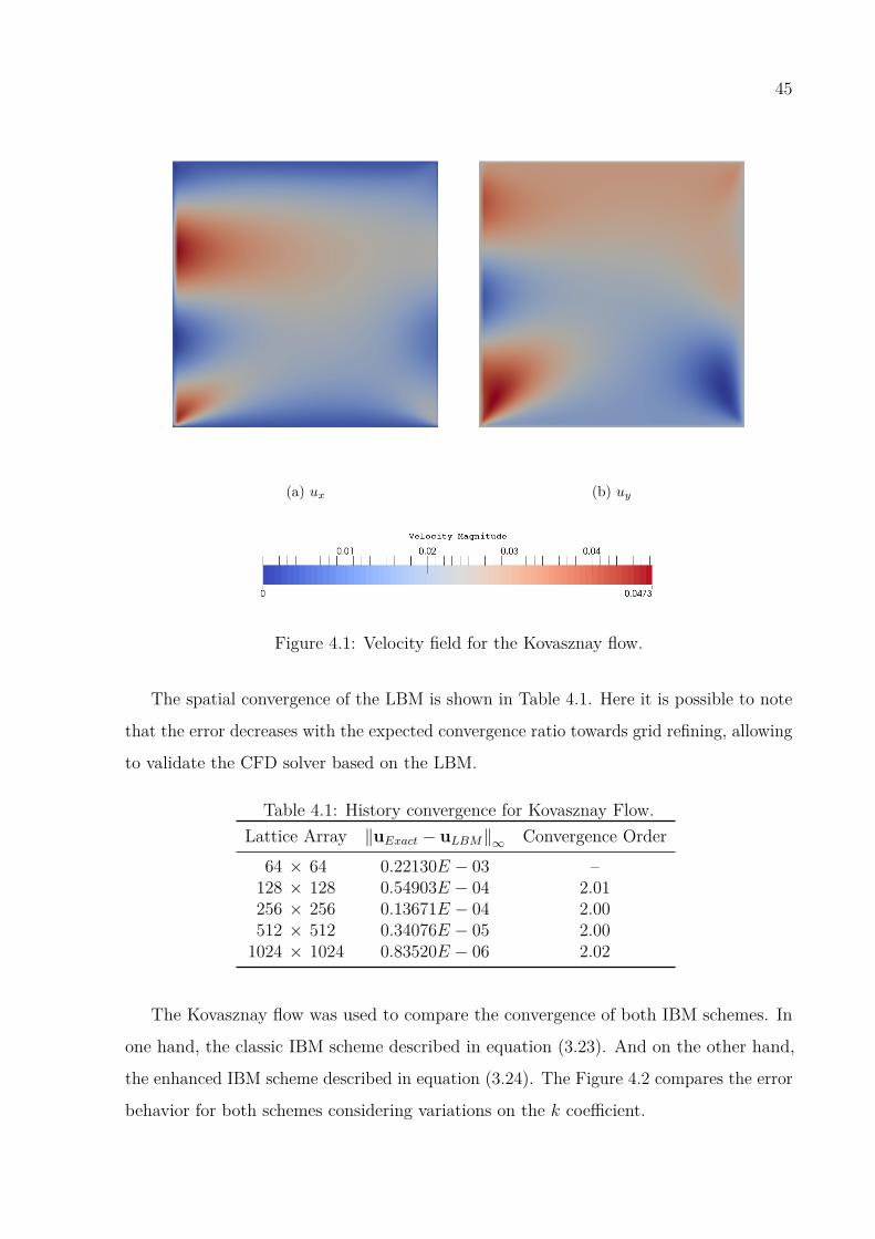
Figure 4.1: Velocity field for the Kovasznay flow.

The spatial convergence of the LBM is shown in Table 4.1. Here it is possible to note

that the error decreases with the expected convergence ratio towards grid refining, allowing

to validate the CFD solver based on the LBM.

Table 4.1: History convergence for Kovasznay Flow.Lattice Array ‖uExact − uLBM‖∞ Convergence Order

64 × 64 0.22130E − 03 –128 × 128 0.54903E − 04 2.01256 × 256 0.13671E − 04 2.00512 × 512 0.34076E − 05 2.00

1024 × 1024 0.83520E − 06 2.02

The Kovasznay flow was used to compare the convergence of both IBM schemes. In

one hand, the classic IBM scheme described in equation (3.23). And on the other hand,

the enhanced IBM scheme described in equation (3.24). The Figure 4.2 compares the error

behavior for both schemes considering variations on the k coefficient.

46

1e-07

1e-06

1e-05

0.0001

0.01 0.1 1

-lo

g(E

rro

r)

k

Classic Scheme

Enhanced Scheme c=k*1E-03

Figure 4.2: Comparison between the classic IBM scheme (3.23) vs. the enhanced IBM

scheme (3.24).

In this comparison it is possible to note that the enhanced scheme for evaluating the

force-like term results more accurate than the classic scheme. Thus, when referring to the

IBM the enhanced method will be addressed.

4.2 Flows with rigid obstacles

In this section, numerical results are presented to validate the LBM for solving the

incompressible Navier-Stokes equations with rigid obstacles. In these studies, well known

important flow coefficients such as drag and lift were studied considering various Reynolds

numbers. The obtained values from numerical simulations were compared with exact

solutions or data from literature.

4.2.1 Flow around a spinning circle

The following experiment attempts to model the inverse Magnus effect employing the

forcing method to impose a spin boundary constraint. This phenomenon takes place when

the bulk flow is modified due to the presence of a spinning obstacle. The obstacle itself

alters the bulk flow, nevertheless if the obstacle spins over its geometrical axis the resultant

flow is non-symmetric. This problem has been studied before by [18, 25, 53, 27], showing

47

a compelling need of computational mechanics to simulate and understand the motion

actions like drag and lift forces when the obstacle rotates.

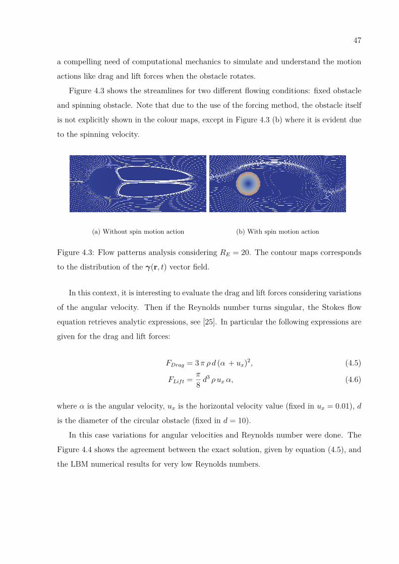
Figure 4.3 shows the streamlines for two different flowing conditions: fixed obstacle

and spinning obstacle. Note that due to the use of the forcing method, the obstacle itself

is not explicitly shown in the colour maps, except in Figure 4.3 (b) where it is evident due

to the spinning velocity.

(a) Without spin motion action (b) With spin motion action

Figure 4.3: Flow patterns analysis considering RE = 20. The contour maps corresponds

to the distribution of the γ(r, t) vector field.

In this context, it is interesting to evaluate the drag and lift forces considering variations

of the angular velocity. Then if the Reynolds number turns singular, the Stokes flow

equation retrieves analytic expressions, see [25]. In particular the following expressions are

given for the drag and lift forces:

FDrag = 3π ρ d (α + ux)2, (4.5)

FLift = π

8 d3 ρ ux α, (4.6)

where α is the angular velocity, ux is the horizontal velocity value (fixed in ux = 0.01), d

is the diameter of the circular obstacle (fixed in d = 10).

In this case variations for angular velocities and Reynolds number were done. The

Figure 4.4 shows the agreement between the exact solution, given by equation (4.5), and

the LBM numerical results for very low Reynolds numbers.

48

0

0.005

0.01

0.015

0.02

0.025

0.03

0.01 0.03 0.05 0.07 0.09

Dra

g f

orc

e

Angular velocity variations

Reference

Re=0.1

Re=1

Re=10

Re=20

0

0.2

0.4

0.6

0.8

1

1.2

1.4

1.6

1.8

2

0.01 0.03 0.05 0.07 0.09

Lift

forc

e

Angular velocity variations

Reference

Re=0.1

Re=1

Re=10

Re=20

Figure 4.4: Drag and lift forces for different Reynolds numbers.

4.2.2 Turek’s Benchmark

The compilation made by Turek and Schafer [59], proposes a broad range of problems

for evaluating the performances of numerical CFD solvers. The problems that Turek and

Schafer proposes in [59] allow to understand flow around a cylinder and assess the results

obtained by different numerical solvers. In this work the first problem of the mentioned

benchmark, entitled as Test case 2D-1 (steady), was studied. The geometry and boundary

conditions for this case are shown in Figure 4.5.

Figure 4.5: Geometry of the flow around a cylinder, the geometry was re-scaled to Lattice

units.

For the Test case 2D-1 (steady) benchmark case the inflow, satisfies the following

expression:

ux = 4ux0

Ny2 y (Ny − y) , uy = 0.0,

49

where ux0 = 0.3. The Reynolds number was fixed in RE = 20.0. For this analysis the

outflow assumed periodic boundary conditions.

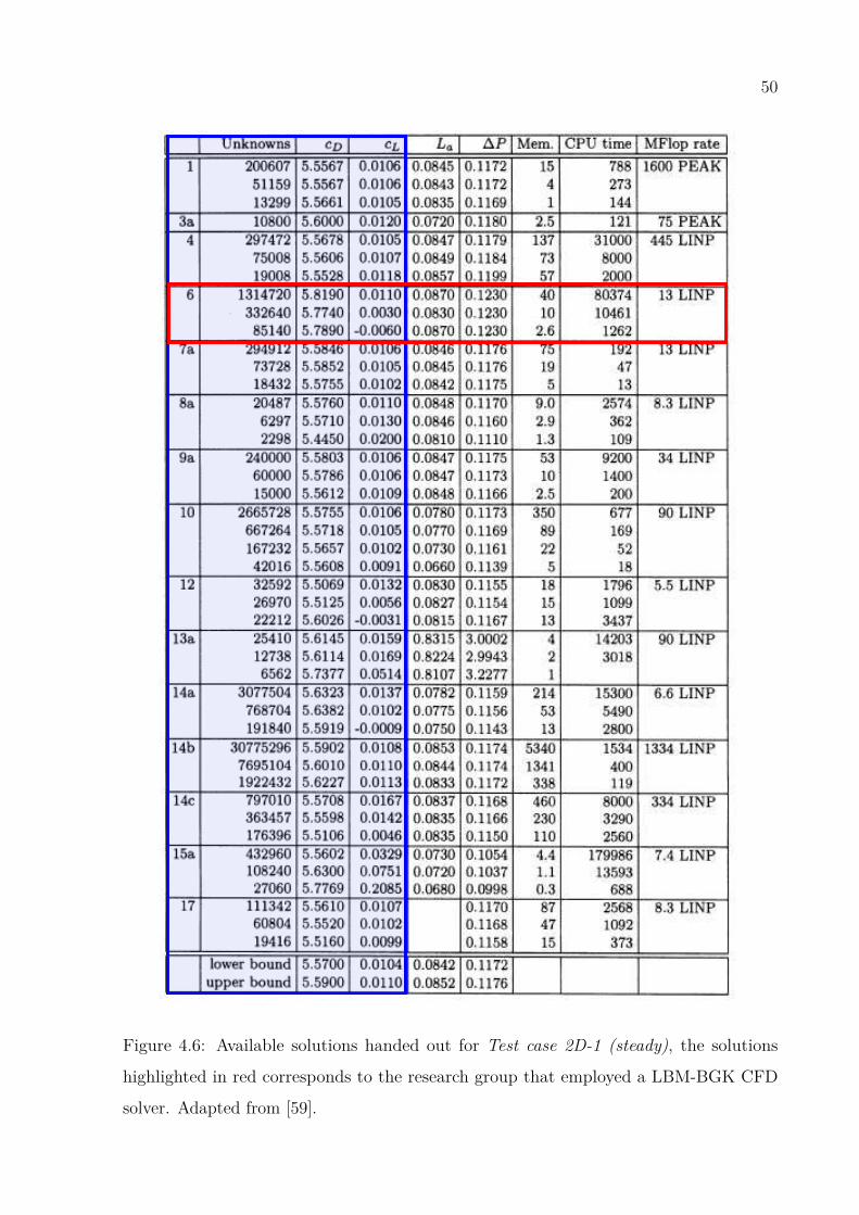
Several research groups obtained solutions for the proposed benchmark problem using

different CFD methods like solvers based on the Finite Difference Method, the Finite

Volume Method, the Finite Element Method and the LBM-BGK. In Figure 4.6 it is

possible to see the solutions that several research groups obtained for the benchmark case

considering some important parameters of the problem under study.

For this experiment, the implemented CFD solver will be compared using the Degrees

of Freedom (#DOF), drag coefficient (CD) and lift coefficient (CL), which are highlighted

in blue in Figure 4.6 for all the participants of the benchmark.

50

Figure 4.6: Available solutions handed out for Test case 2D-1 (steady), the solutions

highlighted in red corresponds to the research group that employed a LBM-BGK CFD

solver. Adapted from [59].

51

Here the drag and lift forces were measured employing the scheme proposed by

Mei et al [38], represented with equation (3.17). The simulations are performed by two

methodologies to represent the inclusion of obstacles. The forcing method of Mohamad [39]

requires a high grid refinement to properly represent the circular cylinder precisely. The

IBM combines two different frames of references (Eulerian references for the fluid and

Lagrangian references for the fluid-solid interface), and therefore is expected to better

represent the circular fluid-solid interface.

Concerning the upper-bounds and lower-bounds shown in Figure 4.6, which are

recommended values for the drag and lift coefficients proposed by Turek and Schafer,

the research group 6 reported solutions employing a LBM-BGK based CFD solver. The

solution obtained by this research group are far away from the solutions obtained with other

numerical methods. In this work, both the forcing method and IBM presents solutions for

the drag and lift coefficient in closer to the available bounds than the one obtained by

group 6 of the Turek’s benchmark. The Figure 4.7 shows a comparison of Forcing method

and IBM to describe the drag and lift coefficients when increasing of the number of degrees

of freedom (#DOF).

5.5

5.55

5.6

5.65

5.7

5.75

5.8

1e+04 1e+05 1e+06 1e+07

Va

lue

s

#DOF

LBM

LBM-IBM

(a) Drag analysis

0.01

0.0105

0.011

0.0115

0.012

0.0125

0.013

0.0135

0.014

0.0145

1e+04 1e+05 1e+06 1e+07

Va

lue

s

#DOF

LBM

LBM-IBM

(b) Lift analysis

Figure 4.7: Forcing method vs IBM, drag and lift analysis.

Both methods resulted in solutions for the drag and lift coefficients in agreement with

the bounds shown in Figure 4.6. In what concerns the computational cost and performance,

the IBM results a method that is more efficient that the Forcing method. From now and

beyond when modeling flows altered with the presence of obstacles the IBM will be used

to simulate the proposed problem.

52

Figure 4.8 compares the contour maps for the velocity obtained employing the forcing

method and the IBM. In this simulations, the forcing method requires 539000 nodes for

the LBM to solve the problem and only 339 Lattices were related to the circular inclusion.

In the forcing method the grid refinement was done in all the computational domain until

the drag coefficient was between the upper and lower bounds, see Figure 4.6. On the other

hand the IBM obtained solutions that required 77000 nodes to solve the problem within

the same accuracy (between lower and upper bounds of the drag and lift coefficients). In

this case, only 52 Lagrangian nodes were used to represent the circular obstacle. In terms

of computational performance, the forcing method requires 200 minutes to complete 10000

iterative steps, while the IBM requires only 81 minutes to complete the simulation.

(a) Forcing method (b) IBM

Figure 4.8: Velocity contour maps comparison. (a) forcing method and (b) IBM.

4.2.3 Flow around a cylinder

In this experiment the LBM-IBM is used to solve the flow around a circular cylinder

subjected to the boundary conditions as described in Figure 4.9. This benchmark problem

was proposed in [13, 38] consisting in a circular cylinder immersed in a rectangular channel

through where the fluid flows.

53

Figure 4.9: Geometry of the flow around a cylinder.

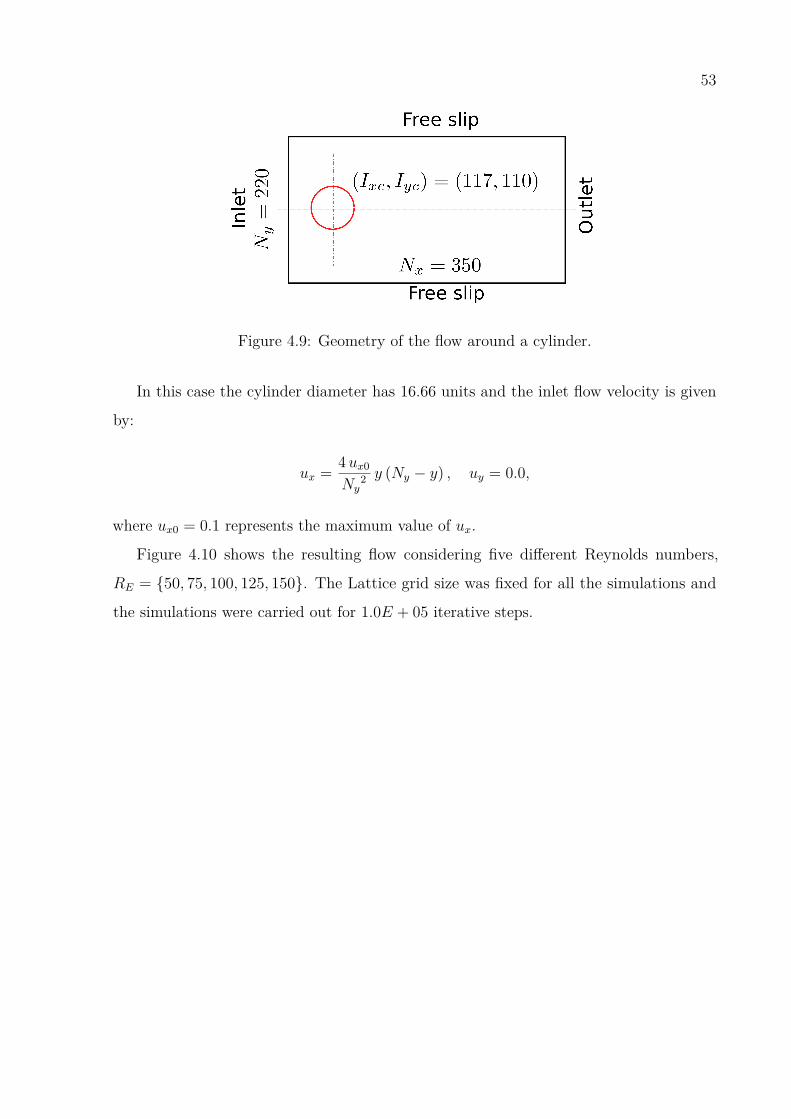
In this case the cylinder diameter has 16.66 units and the inlet flow velocity is given

by:

ux = 4ux0

Ny2 y (Ny − y) , uy = 0.0,

where ux0 = 0.1 represents the maximum value of ux.

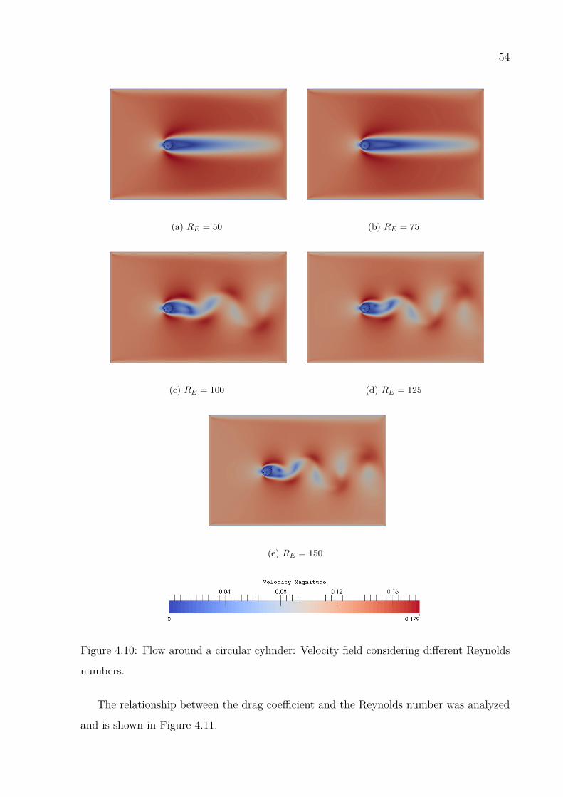
Figure 4.10 shows the resulting flow considering five different Reynolds numbers,

RE = 50, 75, 100, 125, 150. The Lattice grid size was fixed for all the simulations and

the simulations were carried out for 1.0E + 05 iterative steps.

54

(a) RE = 50 (b) RE = 75

(c) RE = 100 (d) RE = 125

(e) RE = 150

Figure 4.10: Flow around a circular cylinder: Velocity field considering different Reynolds

numbers.

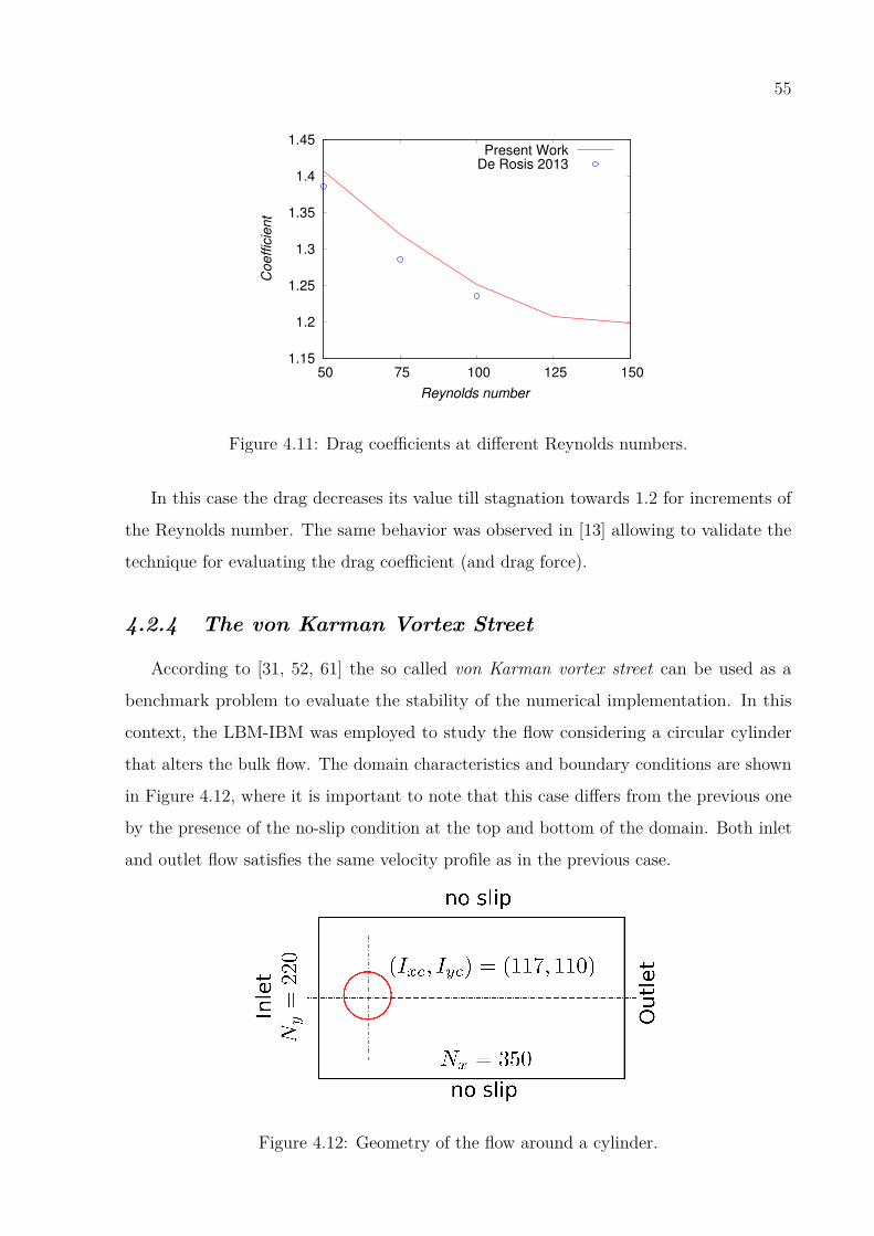
The relationship between the drag coefficient and the Reynolds number was analyzed

and is shown in Figure 4.11.

55

1.15

1.2

1.25

1.3

1.35

1.4

1.45

50 75 100 125 150

Coeffic

ient

Reynolds number

Present Work

De Rosis 2013

Figure 4.11: Drag coefficients at different Reynolds numbers.

In this case the drag decreases its value till stagnation towards 1.2 for increments of

the Reynolds number. The same behavior was observed in [13] allowing to validate the

technique for evaluating the drag coefficient (and drag force).

4.2.4 The von Karman Vortex Street

According to [31, 52, 61] the so called von Karman vortex street can be used as a

benchmark problem to evaluate the stability of the numerical implementation. In this

context, the LBM-IBM was employed to study the flow considering a circular cylinder

that alters the bulk flow. The domain characteristics and boundary conditions are shown

in Figure 4.12, where it is important to note that this case differs from the previous one

by the presence of the no-slip condition at the top and bottom of the domain. Both inlet

and outlet flow satisfies the same velocity profile as in the previous case.

Figure 4.12: Geometry of the flow around a cylinder.

56

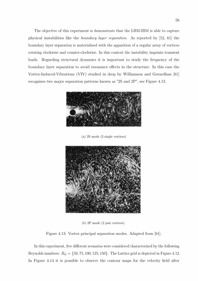
The objective of this experiment is demonstrate that the LBM-IBM is able to capture

physical instabilities like the boundary layer separation. As reported by [52, 61] the

boundary layer separation is materialized with the apparition of a regular array of vortices

rotating clockwise and counter-clockwise. In this context the instability imprints transient

loads. Regarding structural dynamics it is important to study the frequency of the

boundary layer separation to avoid resonance effects in the structure. In this case the

Vortex-Induced-Vibrations (VIV) studied in deep by Williamson and Govardhan [61]

recognizes two major separation patterns known as "2S and 2P", see Figure 4.13.

(a) 2S mode (2 single vortices)

(b) 2P mode (2 pair vortices)

Figure 4.13: Vortex principal separation modes. Adapted from [61].

In this experiment, five different scenarios were considered characterized by the following

Reynolds numbers: RE = 50, 75, 100, 125, 150. The Lattice grid is depicted in Figure 4.12.

In Figure 4.14 it is possible to observe the contour maps for the velocity field after

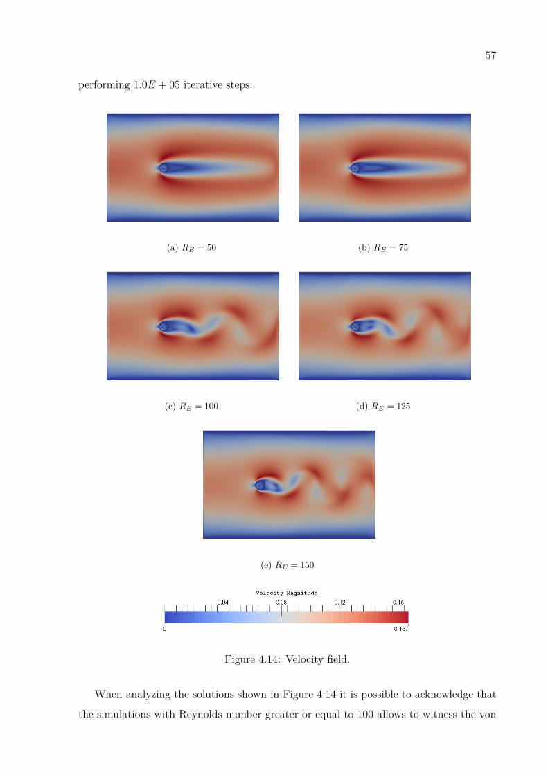
57

performing 1.0E + 05 iterative steps.

(a) RE = 50 (b) RE = 75

(c) RE = 100 (d) RE = 125

(e) RE = 150

Figure 4.14: Velocity field.

When analyzing the solutions shown in Figure 4.14 it is possible to acknowledge that

the simulations with Reynolds number greater or equal to 100 allows to witness the von

58

Karman vortex street effects. The Reynolds number in these cases can be used as a

threshold for analyzing the VIV effects as reported by the works of [31, 52].

Here it is important to characterize the vortex principal separation modes (2S and

2P). To do this the following analysis was done considering three equidistant points with

the labels: "A" representing the node with coordinates (0.25Nx, 0.5Ny), the label "B"

the node with coordinates (0.5Nx, 0.5Ny) and the label "C" the node with coordinates

(0.75Nx, 0.5Ny). These three points allowed to understand effects before the obstacle,

near the obstacle and after the obstacle. The Figures 4.15 and 4.16 shows the variations

of the velocity vector field, components ux and uy, respectively.

-0.1

-0.05

0

0.05

0.1

0.15

0.2

0 5e+04 1e+05

Iterations performed

A

B

C

(a) RE = 50

-0.1

-0.05

0

0.05

0.1

0.15

0.2

0 5e+04 1e+05

Iterations performed

A

B

C

(b) RE = 100

-0.1

-0.05

0

0.05

0.1

0.15

0.2

0 5e+04 1e+05

Iterations performed

A

B

C

(c) RE = 150

Figure 4.15: ux field variations during the simulations.

-0.0035-0.003

-0.0025-0.002

-0.0015-0.001

-0.00050

0.00050.001

0.00150.002

0 5e+04 1e+05

Iterations performed

A

B

C

(a) RE = 50

-0.05

-0.04

-0.03

-0.02

-0.01

0

0.01

0.02

0.03

0.04

0.05

0 5e+04 1e+05

Iterations performed

A

B

C

(b) RE = 100

-0.08

-0.06

-0.04

-0.02

0

0.02

0.04

0.06

0.08

0 5e+04 1e+05

Iterations performed

A

B

C

(c) RE = 150

Figure 4.16: uy field variations during the simulations.

The previous figures allows to distinguish only one frequency of the boundary layer

separation, in deed the frequency corresponds to a vortex separation mode 2S. To conclude

this experiment in Figure 4.17 the density variations are shown for the same three interest

points. The incompressibility constraint was successfully imposed as can be seen from

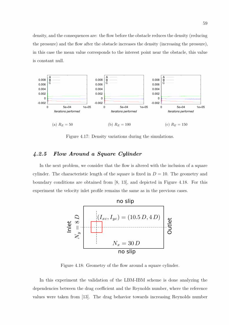
59

density, and the consequences are: the flow before the obstacle reduces the density (reducing

the pressure) and the flow after the obstacle increases the density (increasing the pressure),

in this case the mean value corresponds to the interest point near the obstacle, this value

is constant null.

-0.002

0

0.002

0.004

0.006

0.008

0 5e+04 1e+05

Iterations performed

A

B

C

(a) RE = 50

-0.002

0

0.002

0.004

0.006

0.008

0 5e+04 1e+05

Iterations performed

A

B

C

(b) RE = 100

-0.002

0

0.002

0.004

0.006

0.008

0 5e+04 1e+05

Iterations performed

A

B

C

(c) RE = 150

Figure 4.17: Density variations during the simulations.

4.2.5 Flow Around a Square Cylinder

In the next problem, we consider that the flow is altered with the inclusion of a square

cylinder. The characteristic length of the square is fixed in D = 10. The geometry and

boundary conditions are obtained from [8, 13], and depicted in Figure 4.18. For this

experiment the velocity inlet profile remains the same as in the previous cases.

no slip

Inle

t

Outl

et

no slip

Figure 4.18: Geometry of the flow around a square cylinder.

In this experiment the validation of the LBM-IBM scheme is done analyzing the

dependencies between the drag coefficient and the Reynolds number, where the reference

values were taken from [13]. The drag behavior towards increasing Reynolds number

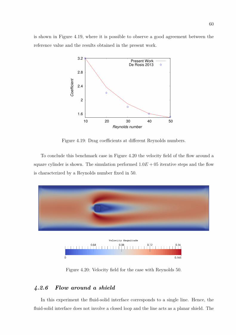
60

is shown in Figure 4.19, where it is possible to observe a good agreement between the

reference value and the results obtained in the present work.

1.6

2

2.4

2.8

3.2

10 20 30 40 50

Coeffic

ient

Reynolds number

Present Work

De Rosis 2013

Figure 4.19: Drag coefficients at different Reynolds numbers.

To conclude this benchmark case in Figure 4.20 the velocity field of the flow around a

square cylinder is shown. The simulation performed 1.0E + 05 iterative steps and the flow

is characterized by a Reynolds number fixed in 50.

Figure 4.20: Velocity field for the case with Reynolds 50.

4.2.6 Flow around a shield

In this experiment the fluid-solid interface corresponds to a single line. Hence, the

fluid-solid interface does not involve a closed loop and the line acts as a planar shield. The

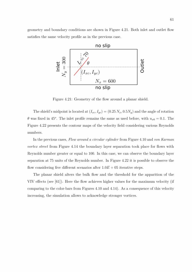
61

geometry and boundary conditions are shown in Figure 4.21. Both inlet and outlet flow

satisfies the same velocity profile as in the previous case.

Inle

t

Outl

et

no slip

no slip

Figure 4.21: Geometry of the flow around a planar shield.

The shield’s midpoint is located at (Ixc, Iyc) = (0.25Nx, 0.5Ny) and the angle of rotation

θ was fixed in 45o. The inlet profile remains the same as used before, with ux0 = 0.1. The

Figure 4.22 presents the contour maps of the velocity field considering various Reynolds

numbers.

In the previous cases, Flow around a circular cylinder from Figure 4.10 and von Karman

vortex street from Figure 4.14 the boundary layer separation took place for flows with

Reynolds number greater or equal to 100. In this case, we can observe the boundary layer

separation at 75 units of the Reynolds number. In Figure 4.22 it is possible to observe the

flow considering five different scenarios after 1.0E + 05 iterative steps.

The planar shield alters the bulk flow and the threshold for the apparition of the

VIV effects (see [61]). Here the flow achieves higher values for the maximum velocity (if

comparing to the color-bars from Figures 4.10 and 4.14). As a consequence of this velocity

increasing, the simulation allows to acknowledge stronger vortices.

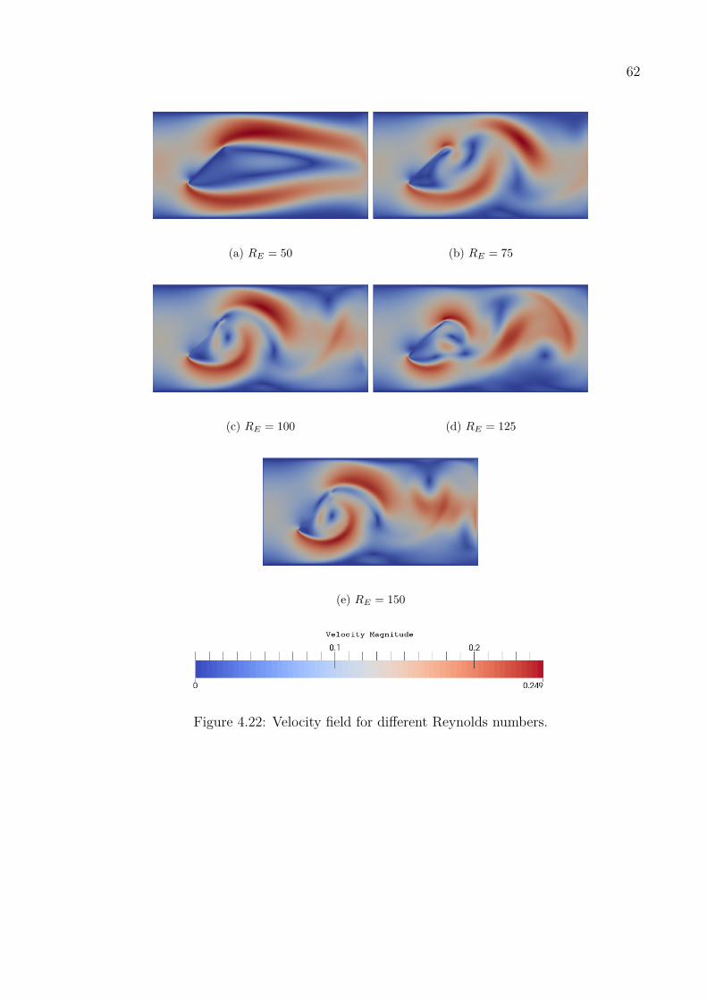
62

(a) RE = 50 (b) RE = 75

(c) RE = 100 (d) RE = 125

(e) RE = 150

Figure 4.22: Velocity field for different Reynolds numbers.

63

5 CONCLUDING REMARKS

In this work a methodology for obtaining the complete set of Euler-Lagrange equations

was presented and employed with focus on fluid-structure interaction problems. This

general modeling procedure is based on three invariant steps concerning: (i) definition of

admissible kinematics; (ii) association of power measures (to perform changes on the pre-

established kinematics); and (iii) characterization of the concept of equilibrium (evoking

the principle of virtual power balance). With a broad range of applications this procedure

was applied to model coupled problems like FSI phenomena.

Focusing on FSI problems the LBM coupled with the IBM were studied and adapted

for performing numerical simulations of fluid flow that concerns rigid obstacles. In this

context, a computational implementation of the methods suitable for FSI problems was

performed and then assessed considering several benchmark problems from the literature.

In this work two different methods were studied to treat obstacles that alters the bulk flow.

In one hand the forcing method of Mohamad [39], which requires a high grid refinement

to accurately represent arbitrary shaped obstacles. On the other hand, the IBM arises as

an alternative representing the arbitrary shaped obstacle with a finite set of Lagrangian

nodes with more accuracy.

The results obtained in the numerical experiments employing the coupling LBM-IBM

solver showed a good agreement with reference values from the literature, indicating

the flexibility in treating more complex geometries easily and still obtaining the desired

accuracy. In some cases the solver presented here obtained results more accurate than

others reported in the literature which were also based on the LBM, as in the problem

from the Turek’s benchmark. Therefore, the LBM-IBM appears as an attractive CFD

solver for studying FSI problems involving complex geometries and flow conditions.

To summarize, it is important to remark the following aspects of the LBM-IBM

methodology used in this work which makes it very attractive for fluid-solid interface

problems:

• the incompressibility constraint for the fluid flow does not represent a challenge

if employing LBM. In numerical techniques like Finite Element Method the

incompressibility of the flow can be imposed employing at least two methods: building

64

up admissible manifolds for the solution field that accounts the free divergence;

or employ Lagrange multipliers to remove from the solution’s manifold the free

divergence constraint. The first alternative "if possible" restricts the range of

admissible solutions to a sharp-small set [49]. The second alternative adds flexibility

to the solution’s manifold but in order ensure numerical stability a functional

dependency must be satisfied, see [9, 51, 50]. In LBM the free divergence constraint

is accounted with the equilibrium distribution, see [11, 24].

• The non-linear convective efforts does not requires linearization iterations. In order

to obtain numerical solutions for the incompressible Navier-Stokes equations the

adopted numerical technique must treat the non-linear term ρu · ∇u. In effect one

can perform Newton-like iterations to linearize the problem. In this context the

convergence of the numerical method can be conditioned not only because of the

problem it-self, but conditioned to the behavior of the Newton-like iterations. In

LBM the explicit framework allows to avoid treating the non-linear convective effects.

• The presence of arbitrary obstacles is computationally viable when employing the

IBM, avoiding excessive grid refinement and resulting in a better approximation of

the geometry. The LBM is defined over an Eulerian Lattice grid, if treating with

arbitrary shaped obstacles the LBM will capture the effects with accuracy only

refining the Eulerian Lattice grid. In other words, this means that the arbitrary

shaped obstacle will have agreement with the Eulerian Lattice grid. The IBM arises

as an alternative for grid refining. In this work a comparison was done of the solution

obtained employing the pure LBM and the IBM technique to treat the presence of

arbitrary shaped obstacles.

• The IBM makes easier to consider other situations, not considered in the present work,

which involves deformable bodies and complex constitutive laws. As a consequence

of representing the fluid-solid interface with a finite set of nodes, it is possible to

study the equilibrium of the nodes considering different numerical scenarios, like

deformations.

65

5.1 Limitations and Future Works

In this work, several assumptions were considered valid for performing numerical

simulations. Here, for granting the stability of the LBM-IBM a pre-processing was done

for every numerical experiment. This stability analysis is done mostly because the LBM

shares the same properties of an explicit solver. Within this context the computational

implementations can be easily achieved, whereas on the other hand the solution can be

easily polluted due to numerical stability. In future works the stability pre-processing can

be replaced with a more robust scheme, see [40, 29] for more details.

In this work the model for fluid flow around a rigid and moving obstacle and the

numerical counterpart (LBM-IBM) were discussed. In this context, future works can be

extended, allowing the obstacle undergo a deformation process (considering for instance

the finite deformation case). For this extension it is necessary to define solid mechanics

kinematics, solid mechanics measures of expended power and include these measures into

appropriate variational principles.

In what concerns the computational environment of this work, every simulation was

performed in a common desktop computer without the use of parallel techniques which are

very handy for LBM solvers. In future works, in order to simulate more realistic problems

the serial implementation shown in this work will require parallel programming.

5.2 Academic Contributions

During the development of the present work, different academic contributions were

published in specialized academic media. More specifically the following material is

available for the academic community:

Articles published in peer-reviewed journals

• Valdez, A. R., Rocha, B. M., & Igreja, I. An RVE-based multiscale modeling method

for constitutive relations. Rheologica Acta, 1–16. Accepted on March the 8th 2017.

http://dx.doi.org/10.1007/s00397-017-1006-3.

Articles published in conference proceedings

• Andrés R. Valdez & Bernardo M. Rocha. A Variational context for FSI simulations

introducing arbitrary Boundary Constraints. In XXII Congreso Sobre Métodos

66

Numéricos Y Sus Aplicaciones ENIEF, 2016.

http://www.cimec.org.ar/ojs/index.php/mc/article/viewFile/5142/5074,

• Andrés R. Valdez. Constitutive Multiscale Modeling of Heat Diffusion, Reaction

Problems. In XXII Congreso Sobre Métodos Numéricos Y Sus Aplicaciones ENIEF,

2016.

http://www.cimec.org.ar/ojs/index.php/mc/article/viewFile/5169/5100

Abstracts published in conference proceedings

• Andrés R. Valdez. On Multiscale Methods to characterize the permeability of

porous media. In 2nd IMPA-InterPore Conference on Porous Media Conservation

Laws, Numerics and Applications, 2016.

http://www.impa.br/opencms/en/eventos/extra/2016_IMPA-INTERPORE/

attach/Abstracts.pdf

67

Bibliography

[1] Artoli, A., Hoekstra, A., Sloot, P.: Mesoscopic simulations of systolic flow in the

human abdominal aorta. Journal of Biomechanics 39(5), 873 – 884 (2006). DOI

https://doi.org/10.1016/j.jbiomech.2005.01.033

[2] Artoli, A.M., Kandhai, D., Hoefsloot, H.C.J., Hoekstra, A.G., Sloot, P.M.A.: Lattice

BGK simulations of flow in a symmetric bifurcation. Future Generation Computer

Systems 20(6), 909–916 (2004). DOI 10.1016/j.future.2003.12.002

[3] Artoli, A.M., Sequeira, A., Silva-Herdade, A.S., Saldanha, C.: Leukocytes rolling

and recruitment by endothelial cells: Hemorheological experiments and numerical

simulations. Journal of Biomechanics 40(15), 3493–3502 (2007). DOI 10.1016/j.

jbiomech.2007.05.031

[4] Benz, M.: Mercedes benz. https://www.mercedes-benz.com/en/mercedes-benz/

innovation/the-new-climatic-wind-tunnels-by-mercedes-benz-video/

(2017). [Online; accessed September 2017]

[5] Berdichevsky, V.: Variational Principles of Continuum Mechanics. Interaction of

Mechanics and Mathematics. Springer Berlin Heidelberg, Berlin, Heidelberg (2009).

DOI 10.1007/978-3-540-88467-5

[6] Berdichevsky, V.: Variational Principles of Continuum Mechanics. Interaction of

Mechanics and Mathematics. Springer Berlin Heidelberg, Berlin, Heidelberg (2009).

DOI 10.1007/978-3-540-88469-9

[7] Bhatnagar, P.L., Gross, E.P., Krook, M.: A Model for Collision Processes in Gases.

I. Small Amplitude Processes in Charged and Neutral One-Component Systems.

Physical Review 94(3), 511–525 (1954). DOI 10.1103/PhysRev.94.511

68

[8] Breuer, M., Bernsdorf, J., Zeiser, T., Durst, F.: Accurate computations of the laminar

flow past a square cylinder based on two different methods: lattice-Boltzmann and

finite-volume. International Journal of Heat and Fluid Flow 21(2), 186–196 (2000).

DOI 10.1016/S0142-727X(99)00081-8

[9] Brezzi, F.: On the existence, uniqueness and approximation of saddle-point problems

arising from lagrangian multipliers. ESAIM: Mathematical Modelling and Numerical

Analysis - Modélisation Mathématique et Analyse Numérique 8(R2), 129–151 (1974)

[10] Campos, J., Oliveira, R., dos Santos, R., Rocha, B.: Lattice boltzmann method for

parallel simulations of cardiac electrophysiology using gpus. Journal of Computational

and Applied Mathematics 295(Supplement C), 70 – 82 (2016). DOI 10.1016/j.

cam.2015.02.008. VIII Pan-American Workshop in Applied and Computational

Mathematics

[11] Chen, S., Doolen, G.D.: LATTICE BOLTZMANN METHOD FOR FLUID FLOWS.

Annual Review of Fluid Mechanics 30(1), 329–364 (1998). DOI 10.1146/annurev.

fluid.30.1.329

[12] Daher, N., Maugin, G.A.: The method of virtual power in continuum mechanics

application to media presenting singular surfaces and interfaces. Acta Mechanica

60(3-4), 217–240 (1986). DOI 10.1007/BF01176354

[13] De Rosis, A.: Fluid-structure interaction by a coupled lattice boltzmann-finite element

approach. D.sc thesis, UNIVERSITÁ DI BOLOGNA (2013)

[14] D’Angelo, C., Zunino, P.: Numerical approximation with nitsche’s coupling of transient

stokes’/darcy’s flow problems applied to hemodynamics. Tech. rep., MOX - Modeling

and Scientific Computing (2010)

[15] Ekeland, I., Témam, R.: Convex Analysis and Variational Problems. Society for

Industrial and Applied Mathematics (1999). DOI 10.1137/1.9781611971088

[16] Favier, J., Revell, A., Pinelli, A.: A lattice boltzmann-immersed boundary method to

simulate the fluid interaction with moving and slender flexible objects. Journal of

Computational Physics 261, 145–161 (2014). DOI 10.1016/j.jcp.2013.12.052

69

[17] Fremond, M.: Non-Smooth Thermomechanics. Springer Berlin Heidelberg, Berlin,

Heidelberg (2002). DOI 10.1007/978-3-662-04800-9

[18] Galindo-Torres, S.: A coupled discrete element lattice boltzmann method for the

simulation of fluid–solid interaction with particles of general shapes. Computer

Methods in Applied Mechanics and Engineering 265, 107–119 (2013). DOI 10.1016/j.

cma.2013.06.004

[19] Gao, H., Li, H., Wang, L.P.: Lattice boltzmann simulation of turbulent flow laden

with finite-size particles. Computers & Mathematics with Applications 65(2), 194 –

210 (2013). DOI 10.1016/j.camwa.2011.06.028. Special Issue on Mesoscopic Methods

in Engineering and Science (ICMMES-2010, Edmonton, Canada)

[20] Germain, P.: The Method of Virtual Power in Continuum Mechanics. Part 2:

Microstructure. SIAM Journal on Applied Mathematics 25(3), 556–575 (1973).

DOI 10.1137/0125053

[21] Germain, P.: Functional Concepts in Continuum Mechanics. Meccanica 33(5), 433–

444 (1998). DOI 10.1023/A:1004304224398

[22] Golbert, D., Blanco, P., Clausse, A., Feijoo, R.: On the search of more stable second-

order lattice-boltzmann schemes in confined flows. Journal of Computational Physics

294, 605–618 (2015). DOI 10.1016/j.jcp.2015.03.065

[23] Goldstein, D., Handler, R., Sirovich, L.: Modeling a no-slip flow boundary with an

external force field. Journal of Computational Physics 105(2), 354 – 366 (1993).

DOI 10.1006/jcph.1993.1081

[24] He, X., Luo, L.S.: Lattice Boltzmann Model for the Incompressible Navier-Stokes

Equation. Journal of Statistical Physics 88(3/4), 927–944 (1997). DOI 10.1023/B:

JOSS.0000015179.12689.e4

[25] Holzer, A., Sommerfeld, M.: Lattice boltzmann simulations to determine drag, lift

and torque acting on non-spherical particles. Computers & Fluids 38(3), 572–589

(2009). DOI 10.1016/j.compfluid.2008.06.001

[26] Iaccarino, G., Verzicco, R.: Immersed boundary technique for turbulent flow

simulations. Applied Mechanics Reviews 56(3), 331 (2003). DOI 10.1115/1.1563627

70

[27] Kim, J., Choi, H., Park, H., Yoo, J.Y.: Inverse Magnus effect on a rotating sphere:

when and why. Journal of Fluid Mechanics 754(2014), R2 (2014). DOI 10.1017/jfm.

2014.428

[28] Kovasznay, L.I.G., Taylor, G.: Laminar flow behind a two-dimensional grid.

Mathematical Proceedings of the Cambridge Philosophical Society 44(01), 58–62

(1948). DOI 10.1017/S0305004100023999

[29] Kruger, T., Kusumaatmaja, H., Kuzmin, A., Shardt, O., Silva, G., Viggen, E.M.:

The Lattice Boltzmann Method. Graduate Texts in Physics. Springer International

Publishing, Cham (2017). DOI 10.1007/978-3-319-44649-3

[30] Li, Z., Favier, J.: A non-staggered coupling of finite element and lattice Boltzmann

methods via an immersed boundary scheme for fluid-structure interaction. Computers

& Fluids 143(November 2016), 90–102 (2017). DOI 10.1016/j.compfluid.2016.11.008

[31] Löhner, R.: Applied Computational Fluid Dynamics Techniques. John Wiley & Sons,

Ltd, Chichester, UK (2008). DOI 10.1002/9780470989746

[32] Maugin, G.A.: Thermomechanical equations of magnetic fluids. International Journal

of Engineering Science 31(1), 27–39 (1993). DOI 10.1016/0020-7225(93)90062-Y

[33] Maugin, G.A.: Continuum Mechanics Through the Twentieth Century, Solid

Mechanics and Its Applications, vol. 196. Springer Netherlands, Dordrecht (2013).

DOI 10.1007/978-94-007-6353-1

[34] Maugin, G.A.: Continuum Mechanics Through the Eighteenth and Nineteenth

Centuries, Solid Mechanics and Its Applications, vol. 214. Springer International

Publishing, Cham (2014). DOI 10.1007/978-3-319-05374-5

[35] Maugin, G.A.: Continuum Mechanics through the Ages - From the Renaissance

to the Twentieth Century, Solid Mechanics and Its Applications, vol. 223. Springer

International Publishing, Cham (2016). DOI 10.1007/978-3-319-26593-3

[36] Maugin, G.A., Trimarco, C.: Note on a mixed variational principle in finite elasticity.

Atti della Accademia Nazionale dei Lincei. Classe di Scienze Fisiche, Matematiche e

Naturali 3(9), 69–74 (1992)

71

[37] McCracken, M., Peskin, C.: A vortex method for blood flow through heart valves.

Journal of Computational Physics 35(2), 183–205 (1980). DOI 10.1016/0021-9991(80)

90085-6

[38] Mei, R., Yu, D., Shyy, W., Luo, L.S.: Force evaluation in the lattice Boltzmann

method involving curved geometry. Physical Review E 65(4), 041,203 (2002). DOI

10.1103/PhysRevE.65.041203

[39] Mohamad, A., Kuzmin, A.: A critical evaluation of force term in lattice Boltzmann

method, natural convection problem. International Journal of Heat and Mass Transfer

53(5-6), 990–996 (2010). DOI 10.1016/j.ijheatmasstransfer.2009.11.014

[40] Mohamad, A.A.: Lattice Boltzmann Method. Springer London, London (2011).

DOI 10.1007/978-0-85729-455-5

[41] Oden, J.T.: An Introduction to Mathematical Modeling: A Course in Mechanics.

John Wiley & Sons (2012)

[42] Oden, J.T., Reddy, J.N.: Variational Methods in Theoretical Mechanics. Universitext.

Springer Berlin Heidelberg, Berlin, Heidelberg (1976). DOI 10.1007/978-3-642-96312-4

[43] Pao, Y.H., Wang, L.S., Chen, K.C.: Principle of virtual power for thermomechanics

of fluids and solids with dissipation. International Journal of Engineering Science

49(12), 1502–1516 (2011). DOI 10.1016/j.ijengsci.2011.05.016

[44] Peskin, C.S.: Flow patterns around heart valves: A numerical method. Journal of

Computational Physics 10(2), 252–271 (1972). DOI 10.1016/0021-9991(72)90065-4

[45] Peskin, C.S.: Numerical analysis of blood flow in the heart. Journal of Computational

Physics 25(3), 220–252 (1977). DOI 10.1016/0021-9991(77)90100-0

[46] Peskin, C.S.: The immersed boundary method. Acta Numerica 11(2002), 479–517

(2002). DOI 10.1017/S0962492902000077

[47] Peskin, C.S., McQueen, D.M.: Modeling prosthetic heart valves for numerical analysis

of blood flow in the heart. Journal of Computational Physics 37(1), 113–132 (1980).

DOI 10.1016/0021-9991(80)90007-8

72

[48] Podio-Guidugli, P.: A virtual power format for thermomechanics. Continuum

Mechanics and Thermodynamics 20(8), 479–487 (2009). DOI 10.1007/

s00161-009-0093-5

[49] Raviart, P.A., Thomas, J.M.: A mixed finite element method for second order elliptic

problems. Lecture Notes in Mathematics 606, 292–315 (1977)

[50] Raviart, P.A., Thomas, J.M.: Primal Hybrid Finite Element Methods for 2nd Order

Elliptic Equations. Mathematics of Computation 31(138), 391 (1977). DOI 10.2307/

2006423

[51] Rockafellar, R.: Convex analysis. Princeton University Press (1972)

[52] Schlichting, H., Gersten, K.: Boundary-Layer Theory. Springer Berlin Heidelberg,

Berlin, Heidelberg (2017). DOI 10.1007/978-3-662-52919-5

[53] Shin, J., Lee, J., Lee, S.: A strain-rate model for a lattice boltzmann bgk model

in fluid-structure interactions. Computers & Fluids 88, 126–135 (2013). DOI

10.1016/j.compfluid.2013.08.009

[54] Taroco, E., Blanco, P., Feijoo, R.: Introducción a la Formulación Variacional de la

Mecánica. Fundamentos y Aplicaciones. LNCC/MCTIC - INCT-MACC (2017)

[55] Truesdell, C.: A First Course in Rational Continuum Mechanics. Academic Press

(1977)

[56] Truesdell, C.: The Elements of Continuum Mechanics. June. Springer Berlin

Heidelberg, Berlin, Heidelberg (1984). DOI 10.1007/978-3-642-64976-9

[57] Truesdell, C., Muncaster, R.G.: Fundamentals of Maxwell’s Kinetic Theory of a

Simple Monatomic Gas: Treated as a Branch of Rational Mechanics. Academic Press

(1980)

[58] Truesdell, C., Noll, W.: The Non-Linear Field Theories of Mechanics / Die Nicht-

Linearen Feldtheorien der Mechanik, Encyclopedia of Physics / Handbuch der Physik,

vol. 2 / 3 / 3. Springer Berlin Heidelberg, Berlin, Heidelberg (1965). DOI 10.1007/

978-3-642-46015-9

73

[59] Turek, S.: Efficient Solvers for Incompressible Flow Problems, Lecture Notes in

Computational Science and Engineering, vol. 6. Springer Berlin Heidelberg, Berlin,

Heidelberg (1999). DOI 10.1007/978-3-642-58393-3

[60] Wen-Shu Jiaung Jeng-Rong Ho, C.P.K.: Lattice boltzmann method for the

heat conduction problem with phase change. Numerical Heat Transfer, Part B:

Fundamentals 39(2), 167–187 (2001). DOI 10.1080/10407790150503495

[61] Williamson, C., Govardhan, R.: VORTEX-INDUCED VIBRATIONS. Annual Review

of Fluid Mechanics 36(1), 413–455 (2004). DOI 10.1146/annurev.fluid.36.050802.

122128

Engineers like examples,

Mathematicians like counter examples.

I’m both.