On-line Robot Adaptationto Environmental Change

Scott LenserCMU-CS-05-165

August, 2005

School of Computer ScienceComputer Science Department

Carnegie Mellon UniversityPittsburgh, PA 15213

Thesis Committee:Manuela Veloso, Chair

Takeo KanadeAnthony Stentz

Minoru Asada, Osaka University, Japan

Submitted in partial fulfillment of the requirementsfor the degree of Doctor of Philosophy.

Copyright c©2005 Scott Lenser

This research was sponsored by the Department of the Interior under contract no. NBCH1040007, theUS Army under contract no. DABT639910013, the US Air Force Research Laboratory under grant nos.F306029820135, F306029720250, F306020020549 and through a generous grant from the Sony Corpo-ration. The views and conclusions contained in this document are those of the author and should not beinterpreted as representing the official policies, either expressed or implied, of any sponsoring institution,the U.S. government or any other entity

Abstract

Robots performing tasks constantly encounter changing environmental conditions. These changesin the environment vary from the dramatic, such as rearrangement of furniture, to the subtle, suchas a burnt out light bulb or a different carpeting. We do not recognize many of these changes,especially subtle changes, but robots do. These changes often lead to the failure of robots. Inthis thesis, we develop an algorithm for detecting these changes. Traditional sensor models donot capture all of the dependencies in the sensor data and are not capable of detecting all typesof signal changes while maintaining a strong probabilistic foundation. This thesis corrects theseshortcomings. We show how detecting the current conditions in which the robot is operating canlead to increased performance and lower failure rates. The methods in this thesis are tested on realtasks performed by a real robot, namely a Sony AIBO robot.

3

4

Acknowledgements

There are many people who helped me produce this thesis document. Without the help of all ofmy friends, family, and colleagues, this thesis document would have never been completed.

I would like to thank my advisor, Manuela Veloso, for having faith in me. Without the resourcesyou provided, this research could have never happened. Without your prodding and suggestions,this work would have never materialized and been completed.

I would like to thank all the members of the Carnegie Mellon AIBO team over the years. Withoutyour work, I wouldn’t have had such a capable software system to work with. Without the expe-riences we shared together, I would have never known to even investigate the problems addressedin this thesis. I would particularly like to thank the primary team members over the years (in noparticular order), James Bruce, William Uther, Elly Winner, Martin Hock, Douglas Vail, SoniaChernova, Maayan Roth, Juan Fasola, Paul Rybski, and Colin McMillen. I would especially liketo thank James Bruce for much of the development of the vision and motion systems without whichthis thesis could not have been completed. James Bruce also contributed many useful code frag-ments which made this thesis easier to implement. I would also especially like to thank DouglasVail for collecting some of the accelerometer data used in this thesis.

I would like to thank Sony Corporation for building truly incredible robots and allowing us to workwith them.

I would like to thank my friends for keeping me sane through the process of finishing my thesis.I would especially like to thank James Bruce, Douglas Vail, Sonia Chernova, and Luisa Lu forproviding much entertainment. I would also like to than Luisa Lu for listening to me complain,keeping me on track, and just generally being there whenever I needed a friend.

I would like to thank my family for having faith in me to finish. They’ve never doubted me for aminute and their confidence helped in rough times.

Finally, I would like to thank all of the researchers that have gone before me. Without their insightsand algorithms, this thesis could not have been built.

5

6

Contents

1 Introduction 19

1.1 Introduction . . . . . . . . . . . . . . . . . . . . . . . . . . . . . . . . . . . . . . 19

1.2 Thesis Problem . . . . . . . . . . . . . . . . . . . . . . . . . . . . . . . . . . . . 20

1.3 Approach . . . . . . . . . . . . . . . . . . . . . . . . . . . . . . . . . . . . . . . 21

1.4 Contributions . . . . . . . . . . . . . . . . . . . . . . . . . . . . . . . . . . . . . 21

1.5 Guide to the Thesis . . . . . . . . . . . . . . . . . . . . . . . . . . . . . . . . . . 22

2 Background 25

2.1 Introduction . . . . . . . . . . . . . . . . . . . . . . . . . . . . . . . . . . . . . . 25

2.2 Robots . . . . . . . . . . . . . . . . . . . . . . . . . . . . . . . . . . . . . . . . . 25

2.3 RoboCup . . . . . . . . . . . . . . . . . . . . . . . . . . . . . . . . . . . . . . . 29

2.4 Software Overview . . . . . . . . . . . . . . . . . . . . . . . . . . . . . . . . . . 30

2.5 Vision . . . . . . . . . . . . . . . . . . . . . . . . . . . . . . . . . . . . . . . . . 32

2.5.1 Low Level Vision . . . . . . . . . . . . . . . . . . . . . . . . . . . . . . . 32

2.5.2 High Level Vision . . . . . . . . . . . . . . . . . . . . . . . . . . . . . . 33

2.5.3 Threshold Learning . . . . . . . . . . . . . . . . . . . . . . . . . . . . . . 38

2.5.4 Vision Summary . . . . . . . . . . . . . . . . . . . . . . . . . . . . . . . 39

2.6 Localization . . . . . . . . . . . . . . . . . . . . . . . . . . . . . . . . . . . . . . 39

2.7 Motions . . . . . . . . . . . . . . . . . . . . . . . . . . . . . . . . . . . . . . . . 39

2.8 Behavior System . . . . . . . . . . . . . . . . . . . . . . . . . . . . . . . . . . . 40

2.9 Hidden Markov Models and Dynamic Bayes Nets . . . . . . . . . . . . . . . . . . 41

2.10 Summary . . . . . . . . . . . . . . . . . . . . . . . . . . . . . . . . . . . . . . . 42

7

3 Environment Identification in Localization 43

3.1 Motivation . . . . . . . . . . . . . . . . . . . . . . . . . . . . . . . . . . . . . . . 43

3.2 Localization . . . . . . . . . . . . . . . . . . . . . . . . . . . . . . . . . . . . . . 47

3.3 Monte Carlo Localization . . . . . . . . . . . . . . . . . . . . . . . . . . . . . . . 51

3.4 Limitations of Monte Carlo Localization . . . . . . . . . . . . . . . . . . . . . . . 61

3.5 Sensor Resetting Localization . . . . . . . . . . . . . . . . . . . . . . . . . . . . 63

3.6 Sensor Resetting Localization Discussion . . . . . . . . . . . . . . . . . . . . . . 64

3.7 Environment . . . . . . . . . . . . . . . . . . . . . . . . . . . . . . . . . . . . . . 66

3.8 Implementation Details . . . . . . . . . . . . . . . . . . . . . . . . . . . . . . . . 68

3.9 Results . . . . . . . . . . . . . . . . . . . . . . . . . . . . . . . . . . . . . . . . . 69

3.10 Conclusion . . . . . . . . . . . . . . . . . . . . . . . . . . . . . . . . . . . . . . 75

3.11 Summary . . . . . . . . . . . . . . . . . . . . . . . . . . . . . . . . . . . . . . . 76

4 Environment Identification in Vision 77

4.1 Introduction . . . . . . . . . . . . . . . . . . . . . . . . . . . . . . . . . . . . . . 77

4.2 Algorithm . . . . . . . . . . . . . . . . . . . . . . . . . . . . . . . . . . . . . . . 79

4.2.1 Off-line Segmentation . . . . . . . . . . . . . . . . . . . . . . . . . . . . 80

4.2.2 On-line Segmentation . . . . . . . . . . . . . . . . . . . . . . . . . . . . 81

4.2.3 Distance Metric . . . . . . . . . . . . . . . . . . . . . . . . . . . . . . . . 82

4.3 Labelling Classes . . . . . . . . . . . . . . . . . . . . . . . . . . . . . . . . . . . 83

4.4 Application . . . . . . . . . . . . . . . . . . . . . . . . . . . . . . . . . . . . . . 84

4.4.1 Test Methodology . . . . . . . . . . . . . . . . . . . . . . . . . . . . . . 84

4.4.2 Results . . . . . . . . . . . . . . . . . . . . . . . . . . . . . . . . . . . . 84

4.5 Limitations . . . . . . . . . . . . . . . . . . . . . . . . . . . . . . . . . . . . . . 86

4.6 Summary . . . . . . . . . . . . . . . . . . . . . . . . . . . . . . . . . . . . . . . 86

8

5 Probable Series Classifier Version 1 89

5.1 Introduction . . . . . . . . . . . . . . . . . . . . . . . . . . . . . . . . . . . . . . 89

5.2 System Model . . . . . . . . . . . . . . . . . . . . . . . . . . . . . . . . . . . . . 90

5.3 Probable Series Classifier Algorithm . . . . . . . . . . . . . . . . . . . . . . . . . 92

5.4 Probable Series Predictor Algorithm . . . . . . . . . . . . . . . . . . . . . . . . . 94

5.5 Evaluation in Simulation . . . . . . . . . . . . . . . . . . . . . . . . . . . . . . . 98

5.5.1 Methodology . . . . . . . . . . . . . . . . . . . . . . . . . . . . . . . . . 98

5.5.2 Results . . . . . . . . . . . . . . . . . . . . . . . . . . . . . . . . . . . . 100

5.6 Evaluation on Robotic Data . . . . . . . . . . . . . . . . . . . . . . . . . . . . . . 104

5.6.1 Methodology . . . . . . . . . . . . . . . . . . . . . . . . . . . . . . . . . 104

5.6.2 Results . . . . . . . . . . . . . . . . . . . . . . . . . . . . . . . . . . . . 105

5.7 Conclusion . . . . . . . . . . . . . . . . . . . . . . . . . . . . . . . . . . . . . . 113

5.8 Summary . . . . . . . . . . . . . . . . . . . . . . . . . . . . . . . . . . . . . . . 113

6 Probable Series Classifier Version 2 115

6.1 Introduction . . . . . . . . . . . . . . . . . . . . . . . . . . . . . . . . . . . . . . 115

6.2 System Model . . . . . . . . . . . . . . . . . . . . . . . . . . . . . . . . . . . . . 116

6.3 Probable Series Classifier Algorithm . . . . . . . . . . . . . . . . . . . . . . . . . 118

6.4 Probable Series Predictor Algorithm . . . . . . . . . . . . . . . . . . . . . . . . . 120

6.5 Evaluation in Simulation . . . . . . . . . . . . . . . . . . . . . . . . . . . . . . . 125

6.6 Evaluation on Robotic Data . . . . . . . . . . . . . . . . . . . . . . . . . . . . . . 129

6.6.1 Methodology . . . . . . . . . . . . . . . . . . . . . . . . . . . . . . . . . 129

6.6.2 Results . . . . . . . . . . . . . . . . . . . . . . . . . . . . . . . . . . . . 129

6.7 Training in the Presence of Feedback . . . . . . . . . . . . . . . . . . . . . . . . . 137

6.8 Evaluation in a Robotic Task . . . . . . . . . . . . . . . . . . . . . . . . . . . . . 138

6.8.1 Methodology . . . . . . . . . . . . . . . . . . . . . . . . . . . . . . . . . 139

6.8.2 Results . . . . . . . . . . . . . . . . . . . . . . . . . . . . . . . . . . . . 141

6.9 Conclusion . . . . . . . . . . . . . . . . . . . . . . . . . . . . . . . . . . . . . . 145

6.10 Summary . . . . . . . . . . . . . . . . . . . . . . . . . . . . . . . . . . . . . . . 146

9

7 Related Work 147

7.1 Introduction . . . . . . . . . . . . . . . . . . . . . . . . . . . . . . . . . . . . . . 147

7.2 Related Work . . . . . . . . . . . . . . . . . . . . . . . . . . . . . . . . . . . . . 148

7.2.1 Probabilistic Approaches . . . . . . . . . . . . . . . . . . . . . . . . . . . 148

7.2.2 Classification . . . . . . . . . . . . . . . . . . . . . . . . . . . . . . . . . 150

7.2.3 Prototypes . . . . . . . . . . . . . . . . . . . . . . . . . . . . . . . . . . 154

7.2.4 Clustering . . . . . . . . . . . . . . . . . . . . . . . . . . . . . . . . . . . 156

7.2.5 Connectionist . . . . . . . . . . . . . . . . . . . . . . . . . . . . . . . . . 156

7.3 Summary . . . . . . . . . . . . . . . . . . . . . . . . . . . . . . . . . . . . . . . 157

8 Conclusions and Future Work 159

8.1 Contributions . . . . . . . . . . . . . . . . . . . . . . . . . . . . . . . . . . . . . 159

8.1.1 Probable Series Classifier Contributions . . . . . . . . . . . . . . . . . . . 160

8.2 Future Work . . . . . . . . . . . . . . . . . . . . . . . . . . . . . . . . . . . . . . 160

8.2.1 Identification of the Number of Environments . . . . . . . . . . . . . . . . 161

8.2.2 Incorporation of Continuous Changes . . . . . . . . . . . . . . . . . . . . 161

8.2.3 Combination with HMM Learners . . . . . . . . . . . . . . . . . . . . . . 161

8.2.4 Incorporation of Learning Modules . . . . . . . . . . . . . . . . . . . . . 161

8.3 Summary . . . . . . . . . . . . . . . . . . . . . . . . . . . . . . . . . . . . . . . 162

10

List of Figures

2.1 A Sony ERS-7 AIBO robot used in testing. . . . . . . . . . . . . . . . . . . . . . 26

2.2 A Sony ERS-210 AIBO robot used in testing. . . . . . . . . . . . . . . . . . . . . 26

2.3 Sony ERS-110 AIBO robots playing soccer. . . . . . . . . . . . . . . . . . . . . . 27

2.4 The Sony quadruped robots playing soccer. . . . . . . . . . . . . . . . . . . . . . 30

2.5 The playing field for the RoboCup 2000 Sony legged robot league. . . . . . . . . . 30

2.6 Overall architecture of the CMPack robot soccer software. . . . . . . . . . . . . . 31

2.7 The threshold map indexing scheme. . . . . . . . . . . . . . . . . . . . . . . . . 33

2.8 The result of classifying images from the robot. Source images on the left, classi-fied images on the right. . . . . . . . . . . . . . . . . . . . . . . . . . . . . . . . 34

2.9 Ball location estimation problem. The distance along the ground (g) is the un-known we wish to solve for. All other variables are either known or estimatedfrom known quantities. The distance to the ball (d) is estimated based off apparentsize in the image and the known characteristics of the camera. This problem isover-constrained. . . . . . . . . . . . . . . . . . . . . . . . . . . . . . . . . . . . 36

2.10 Ball location estimation when distance from robot is uncertain. This estimate isused when the distance cannot be calculated based off apparent size due to the ballbeing partially off the image. . . . . . . . . . . . . . . . . . . . . . . . . . . . . . 37

2.11 Ball location estimation in normal case. This estimate does not use the angle ofthe camera which is often a very noisy estimate. . . . . . . . . . . . . . . . . . . 37

2.12 A Dynamic Bayes Net model of signal generation. . . . . . . . . . . . . . . . . . 42

3.1 Robot starts off lost. See text for explanation. . . . . . . . . . . . . . . . . . . . . 52

3.2 Robot sees a marker to its side. See text for explanation. . . . . . . . . . . . . . . 52

3.3 Robot continues moving to right. See text for explanation. . . . . . . . . . . . . . 53

3.4 Robot sees another marker to its side. See text for explanation. . . . . . . . . . . . 53

11

3.5 Robot starts off lost. See text for explanation. . . . . . . . . . . . . . . . . . . . . 59

3.6 Robot sees a marker to its side. The first density is before the update and the lastis after the update. See text for explanation. . . . . . . . . . . . . . . . . . . . . . 59

3.7 Robot continues moving to right. The first density is before the update and the lastis after the update. See text for explanation. . . . . . . . . . . . . . . . . . . . . . 60

3.8 Robot sees another marker to its side. The first density is before the update and thelast is after the update. See text for explanation. . . . . . . . . . . . . . . . . . . . 60

3.9 The sequence of belief states resulting from a robot in an unknown initial locationseeing one landmark. . . . . . . . . . . . . . . . . . . . . . . . . . . . . . . . . . 65

3.10 Error on real robots versus time. . . . . . . . . . . . . . . . . . . . . . . . . . . . 71

3.11 Deviation reported by localization on real robots versus time. . . . . . . . . . . . . 71

3.12 Simulation error versus number of samples. . . . . . . . . . . . . . . . . . . . . . 72

3.13 Simulation interval error versus number of samples. . . . . . . . . . . . . . . . . . 73

3.14 Simulation SRL and MCL with noise error versus time. . . . . . . . . . . . . . . . 73

3.15 Simulation SRL and MCL without noise error versus time. . . . . . . . . . . . . . 74

3.16 Simulation SRL and MCL interval error versus time. . . . . . . . . . . . . . . . . 74

3.17 Simulation SRL and MCL error versus systematic model error. . . . . . . . . . . . 75

4.1 Robot used in testing. . . . . . . . . . . . . . . . . . . . . . . . . . . . . . . . . . 78

4.2 Image Segmentation Results. The results with adaptation are shown in solid blue.The results using only the bright thresholds are shown with dashed orange lines.In black and white, the adaptation results are black and without adaptation is grey.Each line represents the results from one run on the robot. . . . . . . . . . . . . . . 85

5.1 An example system with three states. . . . . . . . . . . . . . . . . . . . . . . . . . 91

5.2 A Dynamic Bayes Net model of signal generation. . . . . . . . . . . . . . . . . . 93

5.3 Data prediction. The dots in the main graph show the data available for use inprediction. The grey bar shows the range of values used in the prediction. Thebottom graph shows the weight assigned to each model point. The left graph showsthe contribution of each point to the predicted probability of a value at time t asdotted curves. The final probability assigned to each possible value at time t isshown as a solid curve. . . . . . . . . . . . . . . . . . . . . . . . . . . . . . . . . 95

12

5.4 Correlation removal. A linear fit to the model points (shown as dots) is shown.The grey vertical bar shows the range of values actually used in the prediction.The short solid lines show the effect of shifting the model points to match the basevalue of the query while taking into account the correlation. The hollow squaresshow the predicted output values. . . . . . . . . . . . . . . . . . . . . . . . . . . . 99

5.5 Example signal. The first half of the figure shows the baseline sine wave and thesecond half shows the triangle wave. . . . . . . . . . . . . . . . . . . . . . . . . . 101

5.6 Detection of changes to the signal amplitude with equal sized training and testingwindows. The x axis shows the factor by which the amplitude was multiplied. . . . 102

5.7 Detection of changes to the signal mean with equal sized windows. The x axisshows the mean shift as a fraction of the signal amplitude. . . . . . . . . . . . . . 103

5.8 Detection of changes to the observation noise with equal sized windows. The xaxis shows the observation noise as a fraction of the signal amplitude. . . . . . . . 104

5.9 Detection of changes to the period with equal sized windows. The x axis showsthe period of the signal. . . . . . . . . . . . . . . . . . . . . . . . . . . . . . . . . 105

5.10 Detection of changes to the signal amplitude with a fixed training window size.The x axis shows the factor by which the amplitude was multiplied. . . . . . . . . 106

5.11 Detection of changes to the signal mean with a fixed training window size. The xaxis shows the mean shift as a fraction of the signal amplitude. . . . . . . . . . . . 106

5.12 Detection of changes to the observation noise with a fixed training window size.The x axis shows the observation noise as a fraction of the signal amplitude. . . . . 107

5.13 Detection of changes to the period with a fixed training window size. The x axisshows the period of the signal. . . . . . . . . . . . . . . . . . . . . . . . . . . . . 107

5.14 Segmentation between a sine wave and a triangle wave. The y axis shows the logprobability of the sine wave minus the log probability of the triangle wave. Avalue above 0 indicates the signal is probably a sine wave while a value below 0indicates that a triangle wave is more likely. Each data point shows the differencein log probability for the two possible signals based on a window of 25 data pointscentered at the x coordinate of the point. The actual signal was a sine wave fromtimes 0–999 and 2000-2999 and a triangle wave the rest of the time. . . . . . . . . 108

5.15 Use of accelerometer data to distinguish between walking down a ramp, walkingacross a carpet, and walking into a wall. . . . . . . . . . . . . . . . . . . . . . . . 109

5.16 Use of accelerometer data to distinguish between playing soccer, walking into awall, walking with one leg caught on an obstacles, and standing still. . . . . . . . . 110

5.17 Use of average luminance from images to distinguish between bright, medium,dim, and off lights while playing soccer. . . . . . . . . . . . . . . . . . . . . . . . 111

13

5.18 Use of average luminance from images to distinguish between bright, medium,dim, and off lights while standing still. . . . . . . . . . . . . . . . . . . . . . . . . 112

6.1 An example system with three states. . . . . . . . . . . . . . . . . . . . . . . . . . 117

6.2 A Dynamic Bayes Net model of signal generation. . . . . . . . . . . . . . . . . . 118

6.3 Data prediction. The dots in the main graph show the data available for use inprediction. The grey bar shows the range of values used in the prediction. Thebottom graph shows the weight assigned to each model point. The left graph showsthe contribution of each point to the predicted probability of a value at time t asdotted curves. The final probability assigned to each possible value at time t isshown as a solid curve. . . . . . . . . . . . . . . . . . . . . . . . . . . . . . . . . 121

6.4 Detection of changes to the signal amplitude with a fixed training window size.The x axis shows the factor by which the amplitude was multiplied. . . . . . . . . 127

6.5 Detection of changes to the signal mean with a fixed training window size. The xaxis shows the mean shift as a fraction of the signal amplitude. . . . . . . . . . . . 127

6.6 Detection of changes to the observation noise with a fixed training window size.The x axis shows the observation noise as a fraction of the signal amplitude. . . . . 128

6.7 Detection of changes to the period with a fixed training window size. The x axisshows the period of the signal. . . . . . . . . . . . . . . . . . . . . . . . . . . . . 128

6.8 Use of accelerometer data to distinguish between walking down a ramp, walkingacross a carpet, and walking into a wall. . . . . . . . . . . . . . . . . . . . . . . . 132

6.9 Use of accelerometer data to distinguish between walking in place on cement, hardcarpet, and soft carpet. . . . . . . . . . . . . . . . . . . . . . . . . . . . . . . . . 133

6.10 Use of accelerometer data to distinguish between playing soccer, walking into awall, walking with one leg caught on an obstacles, and standing still. . . . . . . . . 134

6.11 Use of average luminance from images to distinguish between bright, medium,dim, and off lights while playing soccer. . . . . . . . . . . . . . . . . . . . . . . . 135

6.12 Use of average luminance from images to distinguish between bright, medium,dim, and off lights while standing still. . . . . . . . . . . . . . . . . . . . . . . . . 136

6.13 Information flow and feedback loops for the ball chasing task. . . . . . . . . . . . 138

6.14 Setup for the ball chasing task. Each waypoint is marked in the image with a blackdot and a numeric identifier. The actual waypoints were marked with clear tape soas not to interfere with the vision of the robot. The robot and ball are visible in thepicture between waypoints 3 and 4. . . . . . . . . . . . . . . . . . . . . . . . . . . 140

14

6.15 Results from the ball chasing task in the forward direction. The x axis shows thewaypoint number. The y axis counts the successes in reaching this waypoint outof 10 runs. . . . . . . . . . . . . . . . . . . . . . . . . . . . . . . . . . . . . . . . 142

6.16 Results from the ball chasing task in the reverse direction. The x axis shows thewaypoint number. The y axis counts the successes in reaching this waypoint outof 10 runs. . . . . . . . . . . . . . . . . . . . . . . . . . . . . . . . . . . . . . . . 142

15

16

List of Tables

3.1 Pseudo-code for updating the set of particles in response to a movement update. . . 55

3.2 Pseudo-code for updating the set of particles in response to a sensor update withoutnormalization. . . . . . . . . . . . . . . . . . . . . . . . . . . . . . . . . . . . . . 56

3.3 Pseudo-code for updating the set of particles in response to a sensor update withnormalization. . . . . . . . . . . . . . . . . . . . . . . . . . . . . . . . . . . . . . 57

3.4 Pseudo-code for SRL for updating the set of particles in response to a sensor update. 64

3.5 Performance summary on real robots. . . . . . . . . . . . . . . . . . . . . . . . . 70

4.1 Off-line Segmentation of Data . . . . . . . . . . . . . . . . . . . . . . . . . . . . 80

4.2 On-line Segmentation of Data . . . . . . . . . . . . . . . . . . . . . . . . . . . . 81

4.3 Labelling Classes . . . . . . . . . . . . . . . . . . . . . . . . . . . . . . . . . . . 83

5.1 Probable Series Predictor algorithm. . . . . . . . . . . . . . . . . . . . . . . . . . 97

5.2 Accuracy of PSC in various test classification tasks. . . . . . . . . . . . . . . . . . 105

6.1 Probable Series Predictor algorithm. . . . . . . . . . . . . . . . . . . . . . . . . . 123

6.2 Accuracy of PSC in various test classification tasks. . . . . . . . . . . . . . . . . . 130

6.3 Training method for Probable Series Classifier. . . . . . . . . . . . . . . . . . . . 137

6.4 Success in a ball chasing task versus thresholds. . . . . . . . . . . . . . . . . . . . 141

6.5 Success rates for reaching waypoints per environment and threshold. . . . . . . . . 144

6.6 Adaptation perfomance compared to best possible threshold. . . . . . . . . . . . . 144

17

18

Chapter 1

Introduction

1.1 Introduction

This thesis focuses on the problem of detecting changing environments in a online, signal-independentmanner and adapting to these changes. We focus on practical solutions that are applicable to a widerange of robotic adaptation problems. We focus on discrete changes to the environment.

Autonomous robots must perceive the world around them, make decisions as to what actions totake, and perform those actions. We are interested in autonomous robots that perform their decisioncycle in real time. Each of these three parts of the decision cycle is a core challenge in designingautonomous robots.

In order to perceive the world, a robot needs a model of its sensors. This model is intrinsic to therobot. An example would be a model for a camera which characterizes the pixel values obtainedby the particularly wavelengths of light hitting the sensor. The robot also needs a model of theworld. This model includes knowledge about what objects are in the world, their characteristics,and how they change over time. An example would be a model which says that the ball of interestto the robot is round and orange. Usually, these two models are combined into one sensor modelwhich maps from raw sensory information to percepts about the world. An example percept wouldbe the location relative to the robot of a ball of interest to the robot.

In order to make decisions, the robot must rely on its perception of the world around it to provideneeded information. The robot must also rely on its actions to successfully modify the environ-ment. Once these requirements are satisfied, the robot can choose an appropriate action to respondto the state of the world to move it towards its goals.

In order to perform actions in the world, the robot must have a model of what effect its actuatorshave on the state of the world. Again, this actuator model combines aspects of the robot and theenvironment. The parts of this model related to the forces generated by the robot’s motors inresponse to commands are intrinsic to the robot. However, the change in the state of the world

19

as a result of these forces depends on the environment. The same motor commands will producedifferent results for a robot travelling over carpeting than one travelling over smooth tiles.

All of these models are crucial to the performance of the robot. This thesis addresses the problemof how to detect changes in the environment and adapt to the change by the selection of appropriatemodels to match the current environment. Furthermore, the thesis aims at detection and adaptationmethods that are online and not dependent on the particular sensor signal to be processed. Thethesis develops detection methods that are probabilistically well-founded, practical, and make noassumptions that aren’t likely to hold in practice.

The rest of this chapter is organized as follows. Section 1.2 details the thesis problem. Section 1.3discusses the approach taken. Section 1.4 describes the contributions from the work. Section 1.5provides an overview of this thesis.

1.2 Thesis Problem

The central question of this thesis is:

Can a robot autonomously use sensors to identify changes in its environment online in asignal-independent manner and adapt to those changes to improve its performance at a task?

By environment, we mean a set of conditions in the world under which the robot is operating. Asingle environment will be consistent enough that a single sensor model plus a single action modelis sufficient to create a behavior which can effectively perform the robot’s task. Environmentscould be position based such as different rooms in a building or attribute based such as the sameroom under different lighting conditions.

We only considerchangesthat result in discrete changes in the environment.

By online, we mean that the current environment can be identified and adapted to in real-time withlow latency. By adaptation, we mean selecting an appropriate sensor and action model to matchthe current environment.

Finally, we focus onsignal-independenttechniques, i.e. those techniques that do not depend onany domain-specific knowledge or make any assumptions that are not typically satisfied in roboticdomains.

We investigate two different methods to improve the robot’s performance:

• Identification of a failure of the robot and execution of a recovery action.

• Identification of the environment to select an appropriate model for the behavior to use.

20

1.3 Approach

We take the approach of creating a general state identification technique to be used to identifythe current environment. We concentrate on validating it on robotic sensor signals. We use onlyinformation that is readily available on robots. Because we don’t want to limit ourselves to one typeof sensor, we make as few assumptions as possible. We focus on a mathematical approach basedon probability theory. By having a strong mathematical basis, the generated technique becomesmore open to analysis and the results more open to interpretation. To further reduce the number ofassumptions required, we base our technique on non-parametric statistics. By using non-parametricstatistics, we free ourselves from assumptions about the distribution of sensor signals and are ableto handle a broader collection of possible sensor signals.

We test the state identification technique in a variety of ways. We test in simulation to verify theability of the technique to discriminate a number of different possible changes that could occurin signals. Testing in simulation allows us to systematically vary the input signals and test theresolution of the system. We then test on a variety of real robot signals. These tests verify thetechnique’s ability to successfully identify environments on real data streams with their more com-plex characteristics than simulated signals. These tests also verify that the types of changes foundin real sensor signals are distinguishable by the technique. We finally test the technique in a realrobot task. This test verifies the technique’s utility in real situations.

1.4 Contributions

The main contributions of this thesis are:

Principle of environment identification and response for failure recovery. We show that theprinciple of environment identification can be used for failure detection and recovery. We demon-strate the utility of environment identification for failure recovery in the context of localization.The change in environment, in this case, is a sudden mismatch between the position the localiza-tion believes the robot to be in and the robot’s true position. In this case the failure detected is asoftware failure. We show that detecting this change can be used to change the model used in thelocalization and improve performance. We show improved performance of the localization systemwhen environment identification is used for failure recovery.

Principle of general environment identification and response to improve robot performance.We show that sensors can be used to identify the current state of the robot’s environment. We showhow this knowledge can be used to improve robot performance. What little work as been donein robotics to adapt to the environment has used heavy domain knowledge to distinguish betweendifferent environments. The remaining work uses identification techniques that do not have therobustness, probabilistic basis, and low latency of the thesis technique.

We demonstrate that the techniques and algorithms in this thesis lead to improved robot perfor-mance. We demonstrate that states can be identified from sensor signals from real robots. We prove

21

that this state identification leads to dramatically improved performance of real robots performingreal tasks. We also demonstrate that identifying and adapting to the environment outperformstrying to perform well in all environments on a real robotic task.

General purpose algorithm for identifying the state of a system.We create a general purposealgorithm for identifying the state of a Markovian system with discrete states from a sensor stream.The algorithm makes very few assumptions, detects a wide variety of types of changes, is easy totrain, trains in real-time, runs in real-time, and has a strong probabilistic basis.

Other approaches do not have all of these properties. Hidden Markov Model approaches are miss-ing a key dependence between neighboring sensor readings produced from the same environment.We prove that ignoring this dependence leads to drastically reduced performance. Alternative tech-niques such as auto-regressive models lack a strong probabilistic foundation which makes themmore difficult to integrate with probabilistic based decision rules. Auto-regressive models are alsoinherently limited in the types of predictions they can make which limits their applicability to do-mains in which the auto-regressive model can successfully predict the next sensor reading withhigh accuracy. The thesis approach requires only that the distribution over next sensor readings isconsistent and continues working even if the next value itself cannot be predicted. Window-basedapproaches inherently add latency to the system which is not the case for the technique in thisthesis. Window-based approaches also require the user to determine an appropriate window sizewhich can not readily be determined by the task at hand.

1.5 Guide to the Thesis

All readers are recommended to start with Chapter 2 for background about the robotic systemused to perform the tests described in the thesis. Chapter 3 provides motivation for the work thatfollows and makes a contribution to robustness in localization. Chapters 4, 5, and 6 follow thedevelopment of an algorithm for environment identification. The final version of the algorithmpresented in Chapter 6 is the most powerful version. Readers that wish to apply these techniquesmay wish to skip directly to this chapter. Chapter 6 has been written such that it may be readwithout reading the previous chapters, but the previous chapters help put the results in context.Chapter 7 describes related work and may be read at any time. Chapter 8 summarizes the thesisand may also be read at any time.

Chapter 2 - Background In this chapter we lay the ground work for the following chapters. Wecover background material needed to understand the thesis. We also discuss the robots, sensors,software, and environments used in the thesis and the important properties of each.

Chapter 3 - Environment Identification in Localization In this chapter we perform a first explo-ration of the principle of environment identification and response in the context of localization. Weexamine the rationale behind the principle. We then apply the principle to the problem of detectionand recovery of localization failure. This application leads to the Sensor Resetting Localization

22

algorithm that outperforms a similar approach which does not apply environment identificationand response.

Chapter 4 - Environment Identification in Vision In this chapter we present an algorithm forenvironment identification. We apply the algorithm to detect lighting conditions for a simple visiontask. We show that detecting the current lighting conditions in this manner can lead to improvedrobot performance.

Chapter 5 - Probable Series Classifier Version 1In this chapter we present version 1 of theProbable Series Classifier algorithm for time series segmentation and environment identification.The Probable Series Classifier algorithm is based heavily on the Probable Series Predictor algo-rithm which is also presented in this chapter. The Probable Series Classifier algorithm is testedfor performance on simulated data to determine the capabilities of the algorithm. The ProbablySeries Classifier algorithm is also tested on robotic data to verify the capabilities of the algorithmfor solving real problems.

Chapter 6 - Probable Series Classifier Version 2In this chapter we present version 2 of the Prob-able Series Classifier algorithm for time series segmentation and environment identification. Thischapter forms the main algorithmic contribution of this thesis. The development of the algorithmin this chapter does not depend on the development in the previous chapter. The tests from theprevious chapter are repeated with the new algorithm. The algorithm is then applied on-line to anon-trivial robotic task and shown to drastically improve the performance of the robot.

Chapter 7 - Related Work In this chapter we discuss the related work to the thesis.

Chapter 8 - Conclusions and Future Work In this chapter we summarize the important resultsand contributions of this thesis. We also give directions for future work.

23

24

Chapter 2

Background

2.1 Introduction

This chapter provides necessary background to better understand the rest of the thesis. This chap-ter is devoted to explaining the robotic system on which the thesis work has been carried out andthe technical background needed to understand the thesis. This robotic system was originally de-veloped for use in the RoboCup Sony legged league which is an international autonomous robotsoccer competition. The section describing the robot and its sensors is particularly important forunderstanding the signals used in this thesis. The section on vision is very important for under-standing the task results in adapting to different lighting conditions.

Section 2.2 describes the robots used for the thesis work. The sensors on the robot and their im-portant properties are also discussed. Section 2.3 describes the environment for which the roboticsystem was initially designed and developed. Section 2.4 then provides an overview of the soft-ware system used. The following sections provide a more detailed discussion of each componentof the robotic system. Section 2.9 provides background on probabilistic models which will be usedin this thesis.

2.2 Robots

We used Sony AIBO robots in the development of this thesis. Our work started with the ERS-110AIBO (Figure 2.3) robots which were generously provided by Sony. We continued our work onthe newer ERS-210 (Figure 2.2) and ERS-7 (Figure 2.1) models. The final testing was all donewith a Sony ERS-7 AIBO robot as pictured in Figure 2.1. The robot is approximately 25cm longand 20cm wide. It stands about 18cm tall at the shoulder and is approximately 25cm tall includingthe head. The robot is commercially available from Sony. Sony has also provided a free softwaredevelopment environment for the AIBOs which is available from their web site. The robot isoutfitted with many actuators, many sensors, and ample processing power.

25

Figure 2.1: A Sony ERS-7 AIBO robot used in testing.

Figure 2.2: A Sony ERS-210 AIBO robot used in testing.

26

Figure 2.3: Sony ERS-110 AIBO robots playing soccer.

The robot has many actuators as follows:

• 18 degrees of freedom controlled by continuous position servos.

– 3 degrees of freedom in each leg in a rotation-rotation-rotation configuration. Tworotation joints are located in the shoulder and one is located in the knee.

– 3 degrees of freedom for positioning the head. These are setup in a tilt-pan-tilt config-uration. The head is capable of panning through180◦.

– 2 degrees of freedom for positioning the tail

– 1 degree of freedom controlling the mouth

These 18 degrees of freedom are each controlled by a PID (proportional integral derivative)controller which attempt to maintain an angle specified by the control software.

• 2 binary degrees of freedom in the ears which allow the ears to be twitched

• A speaker for audio output.

• Over 20 LEDs which are very useful for output.

The robot has many sensors as follows:

• The primary sensor is a CMOS camera which provides color images of resolution 208x160at a rate of 30Hz. Black and white images can be extracted at a resolution of 416x320 butthis feature was not used in this thesis. The camera was used extensively in this thesis.

27

• The robot has a 3-axis accelerometer. This sensor was also used heavily in this thesis. Theaccelerometer provides information about accelerations experienced by the robot (includingthe acceleration due to gravity).

• The robot’s feet are each outfitted with a binary contact switch. These switches were foundto be unreliable with the walk we usually use.

• Each joint has a position sensor for proprioceptive feedback. In addition to reporting theposition of each joint, the duty cycle of the servo controlling the joint is also reported.

• The robot is outfitted with stereo microphones for receiving audio input.

• The robot also has three range sensors. Two range sensors are mounted in the head andpoint where the camera points. One of these sensors is tuned for determining range to closeobjects while the other is tuned for ranging slightly further objects. The last range sensor islocated in the chest and pointed down and forward. It is primarily intended to detect negativeobstacles such as the edge of a table.

The CMOS camera plays an important role in the tests done later in the thesis. Understandingthe camera’s characteristics will lead to a greater appreciation of this thesis. The lens on thecamera provides a somewhat blurry image with significant color aberration in the corners of theimage. The corners of the image have a bluish tint and are darker than the rest of the image. Thecamera image is captured using a rolling shutter which means that different lines of the imageare captured at slightly different times. This rolling shutter results in bending of the image whenthe camera is moving. There is also very significant blurring when the camera is moving. Thesecamera limitations lead to a difficult vision problem. The camera has a field of view of57◦ in thehorizontal direction and45◦ in the vertical direction. The robot must make aggressive use of theability to aim the camera to keep track of the important objects in its environment. The imagescaptured from the camera are provided in YCrCb format. The Y channel of the image providesinformation about the brightness of each pixel and is basically a black and white image. The Crand Cb channels of the image provide color information. The Cr channel provides informationabout the redness of each pixel while the Cb channel does the same for the blueness of each pixel.

The accelerometer is used heavily in tests of this thesis. The accelerometer provides measures ofacceleration in 3 orthogonal directions aligned with the robot’s body. The acceleration is reportedas a floating point number ranging from -2 to +2 time the acceleration of gravity. From examiningthe actual readings provided by the sensor, it is clear that the original signal is actually discretewith 256 levels of values. Nonetheless, the signal is treated as if it is fully continuous in this thesis.The accelerations experienced by the robot are reported at a rate of 125Hz, or every 8ms. Each8ms period is called a frame and includes a measurement for each of the 3 measurement axes. The8ms frames are collected into a set of 4 frames before being sent to the control software. Thesesets of frames are also double buffered. The net result of this setup is that values from 4 timesseparated by 8ms are reported to the control software every 32ms with a delay of between 32msand 64ms.

28

The ERS-7 AIBO model uses a MIPS R4000 processor running at 584MHz. This processor isresponsible for all processing done on the robot. The robot is also equipped with a standard 802.11bwireless networking card. This wireless networking is used in this thesis to allow for extra off-board processing power. All of the basic processing is done on the robot. The experimentalprocessing done in this thesis was largely done off-board for expediency reasons. The computationdone off-board could also be moved onto the robot which some effort at optimizing the code.

2.3 RoboCup

The robotic system on which the thesis work is built was constructed for use in the RoboCup robotsoccer competition [19]. RoboCup is a robot soccer competition and conference which has thestated aim to “By the year 2050, develop a team of fully autonomous humanoid robots that can winagainst the human world soccer champion team”. RoboCup has many leagues which are designedto cover a wide range of the technical challenges that need to be solved by 2050. Almost all of theRoboCup leagues feature fully autonomous robotic systems which play soccer. The soccer gamesfeature a team of robots against another team of robots. This setup creates a challenging problemwhich involved both cooperating and adversarial agents. The presence of adversarial agents leadsto a very fast-paced game where time to act must be highly optimized. The robots are completelyon their own once the game starts. Humans are not allowed to guide the robots in any manner. Thisautonomy plus the number of games played requires very robust designs in order to do well in thecompetition.

The intermediate goal of RoboCup is to advance the state of the art in robots. By advancing thestate of the art, it is hoped that the final goal for 2050 can be achieved. Towards this end, the rulesof each league change each year to encourage more robust solutions that work in more and morenatural environments. The apparent skill of the robots at playing soccer can improve or degradefrom year to year as the robots are faced with new challenges from changes to the rules.

Our robotic system was designed for the RoboCup legged league. The legged league uses a stan-dard hardware platform and the entries are differentiated by the software used. The league usesthe Sony AIBO robot as the standard hardware platform. As Sony has released improved models,the league has moved to the newer robots as the new standard platform. The league currently usesthe ERS-7 AIBO model. This platform was used for all of the robotic testing in this thesis. In thelegged league, modifications to the hardware are strictly forbidden. This restriction puts all of theteams on an equal footing in terms of hardware and encourages software development and sharingof software. All of the processing and sensing for this league is strictly on the robots. The robotscan communicate with each other via wireless LAN, but communication with off-board computersis strictly forbidden.

Figure 2.4 shows a picture from 2000 of the ERS-110 AIBO robots playing soccer. A schematicof the field from 2000 is shown in Figure 2.5. The robots play with an orange ball with a diameterof 85cm. The ball is made of plastic and is fairly slippery. The robots recognize the ball based on

29

Figure 2.4: The Sony quadruped robots playing soccer.

Robot A team : Blue Robot B team : Red Ball : Orange

Light Blue

Light Blue

Pink

G�oal(Light Blue)

G�oal(Yellow)

G�reen

G�reen

Pink

Pink

Pink

Pink

PinkYellow

Yellow

Field(Green)

Figure 2.5: The playing field for the RoboCup 2000 Sony legged robot league.

its color. The field is constructed of thin green carpeting. The green color of the carpeting helps toidentify the playing surface. The goals are also color coded with one team attempting to score onthe cyan goal and the other on the yellow goal. There are several markers placed around the fieldto help the robots identify their location on the field. These markers consist of colored cylinders inpredefined locations relative to the field. Each marker has two colors placed on top of each other.The colors used on each marker plus the relative position of the colors uniquely identifies eachmarker. The robots are marked by color uniforms made of sticky colored patches. The field hasbeen surrounded by a wall from 1999 to 2004, but the field wall is being removed for 2005. Thenumber of markers has been reduced from an initial 6 markers to the present 4 markers. The sizeof the field has grown from an initial size of 2.8m by 1.8m to a current size of 5.4m by 3.6m.

2.4 Software Overview

The software system on the robots was initially developed for the purposes of competing in theRoboCup legged league. Our entry into the RoboCup legged league is called CMPack. The overallarchitecture of the CMPack software is shown in Figure 2.6. The software is composed of several

30

Vision

Motion

Behaviors

Localization

Location Objects

Objects

Motion updates

Commands

Images

Camera/color segmentation

Figure 2.6: Overall architecture of the CMPack robot soccer software.

interacting cooperating modules. The overall goal of the software is to collect information fromcamera images and use that information to select appropriate motion commands.

The main modules of the system are:

Vision The vision module is responsible for extracting information from camera images. Thevision system takes camera images as input. The primary output of the vision system is alist of objects seen in each camera image (frame). For each object, the vision system reportswhether it was seen, the confidence that it was seen, and the estimated location of the object.The objects seen are used by the behaviors and localization modules.

Localization The localization module is responsible for determining the position of the robot onthe RoboCup field. Localization takes observations of landmarks from vision and infor-mation about motions executed (motion updates) from motion as input. Localization thenreports the estimated position of the robot on the field and the expected error in this estimate.The output of localization is used in behaviors.

Behaviors The behavior system is responsible for deciding what the robot should do. The be-havior system uses the objects seen in the image from vision (primarily the ball) and theestimated position of the robot from localization as inputs. The behavior system selects amotion command to be executed by the motion module. Typical commands are execute akick or walk at a certain velocity and angular velocity. The behavior system also instructsthe motion system on where to position the robot’s head.

31

Motion The motion system is responsible for locomotion and manipulation. The motion systemtakes instructions from the behaviors on what motion would be good to execute. The motionsystem then determines the closest motion that can actually be performed while maintainingbalance and continuity constraints. Once a motion has been selected, the motion systemoutputs target angles for each joint to the operating system to be used by the robot’s built-inservo controllers. The motion system also reports the movements executed to the localizationas an estimate of the change in the robot’s pose.

These modules work together to control the robot based on the feedback from the robot’s camera.The operation of each module is discussed in more detail in the sections that follow.

2.5 Vision

The vision system is responsible for interpreting data from the robots’ primary sensor, a cameramounted in the nose. The images are digitized in the YCrCb color space [50]. The vision moduleis responsible for converting raw YUV camera images into information about objects that therobot sees. This is done in two major stages. The low level vision processes the whole frame andidentifies regions of the same symbolic color. We use CMVision [6, 5] for our low level visionprocessing. The high level vision uses these regions to find objects of interest in the image. Therobot uses a 208 by 160 image size exclusively. The low level vision system and initial thresholdlearning code was largely developed by James Bruce. Scott Lenser is responsible for most of thehigh level vision and the current threshold learning code.

2.5.1 Low Level Vision

The low level vision converts raw YCrCb camera images into 4-connected regions of the samesymbolic color. It does this in several stages. The image is first segmented according to a thresholdtable. This converts each pixel from a YCrCb value to a symbolic color like orange. The colorsegmented image is then run length encoded to reduce the amount of memory consumed by theimage and speed further processing. The run length encoded (RLE) image is then analyzed to find4-connected regions of the same color. Some noise is then removed by merging nearby regions ofthe same color.

Color Segmentation

The robot uses a 3D lookup table for color segmenting the image. The lookup table is indexedby the high bits of the raw Y, Cr (U), and Cb (V) values of the pixel. The number of bits usedfrom each component is configurable. We used 4 bits of Y and 6 bits each of U and V at thecompetition for a total of 16 bits. The indexing scheme is shown graphically in Figure 2.7. This

32

MSB LSB

Y U

V

MSB

MSB

LSB

LSB

Index

Figure 2.7: The threshold map indexing scheme.

yields a lookup table of size 65536 bytes. Each entry of the lookup table stores the index numberfor the symbolic color to assign to the pixel or 0 if the pixel is background. The thresholds arelearned from example images as described in section 2.5.3. The color segmentation process usesthe threshold table on each pixel of the image to produce a color map (cmap) for the image (seeFigure 2.8 for the effect of this process). This cmap image is available to the high level vision tocheck the symbolic color of individual pixels. We treat the field green and the marker green as thesame color when segmenting.

Region Generation

The cmap image is then processed to find 4-connected components which we refer to as regions.This process is done in an efficient manner involving creating a run length encoded version of theimage. Each region contains a list of the runs found in the region. Nearby regions are joined usinga simple heuristic to combat noise. The regions are sorted by color and size and summary statisticsare calculated for each region. The summary statistics include bounding box, centroid, and area.

2.5.2 High Level Vision

The job of high level vision is to find objects of interest in the camera image and estimate theposition of these objects relative to the robot. The high level vision has access to the originalimage, the colorized (cmap) image, the run length encoded (RLE) image, and the region data

33

Figure 2.8: The result of classifying images from the robot. Source images on the left, classifiedimages on the right.

34

structures from the low level vision in order to make its decisions. The region data structures formthe primary input to the high level vision. The high level vision also gets input from the motionmodule in order to calculate the pose of the camera. The parameters sent from the motion object(via shared memory) are the body height, body angle, head tilt, head pan, and head roll. The highlevel vision looks for the ball, the goals, the markers, and the robots. For each object, the visioncalculates the location of the object, the leftmost and rightmost angles subtended by the object, aconfidence in the object, and a confidence that the IR sensor is pointing at the object. The locationof the object is a 3D location relative to a point on the ground directly beneath the base of therobot’s neck. These position calculations are based upon a kinematic model of the head whichcalculates the position and pose of the camera relative to this designated point. The confidence inthe object is a number between 0 and 1 which indicates how well the object fits the expectationsof the vision system, 0 indicating definitely not the object and 1 indicating no basis for saying it isnot the object. The IR sensor confidence is similar. The following sections explain how the variousobjects in the image are located.

Ball Detection

The ball is found by scanning through the 10 largest orange regions and returning the one with thehighest confidence of being the ball.

Confidence Calculation The confidence is based on a bunch of components multiplied togetherplus an additive bonus for having a large number of orange pixels. The following filters are used:

• A binary filter which checks that the ball is tall enough (3 pixels), wide enough (3 pixels),and large enough (7 pixels).

• A real-valued filter which checks that the bounding box of the region is roughly square withGaussian falloff as the region gets less square. Regions on the edge of the image are givenmore lenience.

• A real-valued filter which checks that the area of the region compared to the area of thebounding box matches that expected from a circle. Again, Gaussian falloff is used. Regionson the edge of the image are given more lenience.

• Two filters based on a histogram of the pixel colors of all pixels which are exactly 3 pixelsaway from the bounding box of the region. The first filter is designed to filter out orangefringe on the edge of the red uniforms for robots in the yellow goal. It is not clear if it iseffective. The second filter is designed to make sure that the ball is mostly surrounded bythe field, the wall, or other robots and not the yellow goal.

• NewA real-valued filter based upon the divergence in angle between the two different loca-tion calculation methods (see below).

35

r

dh

camera

a

g

Figure 2.9: Ball location estimation problem. The distance along the ground (g) is the unknown wewish to solve for. All other variables are either known or estimated from known quantities. The dis-tance to the ball (d) is estimated based off apparent size in the image and the known characteristicsof the camera. This problem is over-constrained.

These filters are multiplied together to get the confidence of the ball. The confidence is thenincreased by the number of pixels divided by 1000 to ensure that we never reject really close balls.The ball is then checked to make sure it is close enough to the ground. The robot rejects all ballsthat are located more than5◦ above the robot’s head. The highest confidence ball in the image ispassed on to the behaviors.

Location Calculation The location of the ball relative to the robot is calculated by two differentmeans. The overall problem of estimating the ball position is shown in Figure 2.9. Both methodsrely on the kinematic model of the head to determine the position of the camera. The first methoduses the size of the ball in the image to calculate distance. Geometry is used to solve for the distanceto the ball using the position of the camera relative to the plane containing the ball and the estimateddistance of the ball. This method is shown in Figure 2.11. The disadvantage of this method is thatit assumes that the ball is always fully visible which obviously isn’t always true. The advantage isthat is less sensitive to errors in the position of the camera. The second method uses a ray projectedthrough the center of the ball. This ray is intersected with a plane parallel to the ground at the heightof the ball to calculate the position of the ball. This method is shown in Figure 2.10. The advantageof this method is that its accuracy falls off more gracefully with occlusions or balls off the edgeof the frame. The disadvantage is that it can be numerically unstable if the assumption that theball and robot are on the ground is violated. The distance estimate is also slightly noisier thanthe image size based method but only mostly at large distances. The robot uses the first methodwhenever possible and the divergence between them is factored into the confidence.

36

r

h

camera

a

g

Figure 2.10: Ball location estimation when distance from robot is uncertain. This estimate is usedwhen the distance cannot be calculated based off apparent size due to the ball being partially offthe image.

r

dh

camera

g

Figure 2.11: Ball location estimation in normal case. This estimate does not use the angle of thecamera which is often a very noisy estimate.

37

Marker Detection

Markers are detected by considering all pairs of pink and yellow/green/cyan regions out of thelargest 10 regions of each color. The most confident marker readings are passed along to thebehaviors/localization.

Confidence Calculation The confidence in a marker reading is based upon the following real-valued filters:

• The cosine of the angular spread between the projection of the ray through the center of thetwo colored regions projected onto the ground plane. This filter is setup to fall to 0 at anangular separation of15◦.

• The relative size of the two colored regions (we expect them to be the same size).

• The average size of the two colored regions relative to the square of the distance betweenthem (we expect these values to be equal).

Location Calculation Two rays are projected through the centers of the colored regions. Theserays are made coplanar by projecting both rays onto a vertical plane containing a ray formed byaveraging the two rays. The location of the center of the top of the marker is constrained to be10cm above the center of the bottom of the marker. The location of the top of the marker isalso constrained to be directly vertically above the bottom of the marker. The resulting system ofequations is solved for the location of the marker.

2.5.3 Threshold Learning

Low level vision requires a threshold map from raw YCrCb pixel values to symbolic color. Thresh-old learning is used to create this threshold map. The goal of threshold learning is to take a set ofhand labelled images and produce a threshold map. The threshold map should generalize from thedata as much as possible while correctly classifying as many pixels as possible. The threshold mapis a 3D table of color indices indexed by the high bits of YCrCb pixels. The basic idea is to spreadeach pixel of data out across the entire table giving it more weight closer to its actual value andmuch less weight further away. In order to do this efficiently, we use a mathematically simple formof falloff for each pixel. The weight of each pixel falls off exponentially with Manhattan distancefrom the actual data point. Weights are calculated for each color separately. The final step is todetermine the color to make each cell of the threshold map. This is simply done by looking forthe color with the most weight in each cell. This color is assigned to the cell if its proportion ofthe weight is higher than a user set confidence threshold for the color. Any cell not meeting thiscriterion or with a preponderance of background color is labelled background. This representationand learning method allows us to handle colors with arbitrary distributions including concave anddisjoint distributions.

38

2.5.4 Vision Summary

We find our vision system to be generally robust to noise and highly accurate in object detectionand determining object locations at the RoboCup competition. However, like many vision systemsit remains sensitive to lighting conditions, and requires a fair amount of time and effort to calibrate.

2.6 Localization

The localization module is responsible for determining the position of the robot on the RoboCupfield. It takes objects seen from vision and movements executed from motion and outputs the po-sition of the robot and a confidence on this position. The localization system is based off a proba-bilistic belief state of the robot’s position which is updated as new information becomes available.The probabilistic localization algorithm we developed, Sensor Resetting Localization [38], ro-bustly accommodates the poorly modeled movements of the quadruped robot and large errors dueto externally caused movements of the robots, such as pushing from other robots, and repositioningdone by the human referees during the game. Sensor Resetting Localization is very effective. Thelocalization system is discussed in more detail in Chapter 3.

2.7 Motions

The motion system was largely developed by James Bruce with more recent additions from SoniaChernova and Juan Fasola amongst others.

The motion system for CMPack has to balance requests made by the action selection mechanismwith the constraints of the robot’s capabilities and requirement for fast, stable motions. The desir-able qualities of such a system are to provide stable and fast locomotion, which requires smoothbody and leg trajectories, and to allow smooth, unrestricted transitions between different types oflocomotion and other motions (such as object manipulation). The motion system is given requestsby the behavior system for high level motions to perform, such as walking in a particular direction,looking for the ball with the head, or kicking using a particular type of kick. We decided to im-plement our own motions for the robots so that we would have full parameterization and control,which is not available using the default motions provided with the robot. The system we used forCMPack was based on the design we developed in a previous year [37].

The walking system implemented a generic walk engine that can encode crawl, trot, or pace gaits,with optional bouncing or swaying during the walk cycle to increase stability of a dynamic walk.The walk parameters were encoded as a 51 parameter structure. Each leg had 11 parameters; theneutral kinematic position (3D point), lifting and set down velocities (3D vectors), and a lift timeand set down time during the walk cycle. The global parameters were the z-height of the bodyduring the walk, the angle of the body (pitch), hop and sway amplitudes, the z-lift bound for front

39

and back legs, and the walk period in milliseconds. In order to avoid compilation overhead duringgait development, the walk parameters could be loaded from permanent storage on boot up. Thissystem also allowed us to use different sets of parameters for different motions. Specifically, oneset of parameters was used for motions with a large rotation component, and a different set wasused for straight-line motions. Using two sets of parameters allowed us to optimize each for itsparticular function resulting in faster, more stable movement. In order to switch between motionparameters on the fly while maintaining stability, parameters were selected to be as similar aspossible without compromising their individual effectiveness. Using this interface, we developeda semi-dynamic trotting gait with a maximum walking speed of 300 mm/sec forward or backward,200 mm/sec sideways, or 2.2 rad/sec turning.

Additional motions could be requested from a library of motion scripts stored in files. This ishow we implemented get-up routines and kicks, and the file interface allowed easy developmentsince recompilation was not needed for modifications to an existing motion. Adding a motion stillrequires recompilation, but this is not seen as much of a limitation since code needs to be added tothe behaviors to request that that motion be used.

The overall system was put together using a state machine that included states for walking, stand-ing, and one for each type of kick and get-up motion. Requests from the behaviors would executecode based on the current state that would try to achieve the desired state, maintaining smoothnesswhile attempting to transition quickly.

The technique we used in implementing the walk was to approach the problem from the point ofview of the body rather than the legs. Each leg is represented by a state machine; it is either downor in the air. When it is down, it moves relative to the body to satisfy the kinematic constraintof body motion without slippage on the ground plane. When the leg is in the air, it moves to acalculated positional target. The remaining variables left to be defined are the path of the body,the timing of the leg state transitions, and the air path and target of the legs when in the air. Usingthis approach smooth parametric transitions can be made in path arcs and walk parameters withoutvery restrictive limitations on those transitions.

2.8 Behavior System

The behavior system is responsible for mapping from information about the world to an action toexecute. The input to the system is information about the objects seen (from the vision) and anestimate of the robots location (from the localization). The output of the behaviors is a motion to beexecuted. The motion can be a type of kick to execute (discrete) or a direction to walk (continuous)for example. Developing robust behaviors for robots is a challenge. We use a simple but robustand easy to use control strategy based upon the use of finite state machines.

The behavior system is implemented as a hierarchical collection of finite state machines. Theuppermost finite state machine is responsible for decisions such as attack or defend while lowerlevels are responsible for progressively finer grained decisions. Each state within a state machine

40

corresponds to a policy to follow. A state can either be a reactive behavior or contain a lowerlevel finite state machine. Each state provides a mapping from information about the world to anaction to execute. For instance, one state could correspond to approaching the ball while anotherwould implement searching for the ball. The transitions between states are triggered based uponthe information about the world. Each state transition has a boolean predicate associated with itthat if true causes the current state of the finite state machine to change.

2.9 Hidden Markov Models and Dynamic Bayes Nets

A Hidden Markov Model (HMM) is a system model for time series data. The model consists of:

• A set of possible statess1, . . . , sn.

• A set of possible observationsx1, . . . , xm.

• A transition probability from each state to each stateP (St = si|St−1 = sj).

• A observation probability from each stateP (Xt = xi|St = sj).

The model assumes that the system is composed of some numbern of discrete states. The currentstate of the systemSt is always one of these discrete possibilities. The system is assumed to beMarkovian. A Markov system is one in which knowing the past history of the system provides nonew information if the current state of the system is known. The current state of the system transi-tions according toP (St = si|St−1 = sj) which is time invariant. The observations are all assumedto depend only on the current state of the system. The particular observation seen will depend onthe current state according toP (Xt = xi|St = sj) which is assumed to be time independent. Thisoutput distribution can be extended to the continuous case by assuming a combination of Gaus-sians (or through other means). A detailed tutorial [51] has been produced by Rabiner. Readersunfamiliar with HMMs are encouraged to read a tutorial on them.

A Dynamic Bayes Net (DBN) is a graphical way of representing conditional independence assump-tions amongst random variables. A thorough discussion of DBNs is available in Kevin Murphy’sthesis [45]. General purpose algorithms for analysis in DBNs are available, but all of the algorithmsused in this thesis are derived in this thesis. The basic idea behind a DBN is to represent conditionaldependence between two random variables as an edge in a graph of random variables. Variableswhich are not connected by an edge in this graph (or DBN) are assumed to be independent. Thisthesis uses a simple DBN model to model time series. The model used in this thesis is shown inFigure 2.12. The state of the system at different times is shown asS(j− 2), S(j− 1), S(j) and theobservations at different points in time are shown asX(j − 2), X(j − 1), X(j). With the removalof the large, red arrows, this model makes the same independence assumptions as the standardHMM model. The large, red arrows which are particular to this thesis work are very important formodeling the interdependence of sensor readings from nearby points in time.

41

Figure 2.12: A Dynamic Bayes Net model of signal generation.

2.10 Summary

In this chapter, we described the robotic system on which the thesis work has been carried out. Wedescribed the characteristics of the robot which affect the sensor signals received and the ability ofthe robot to perform different tasks. We also described the software system used on the robot. Wepresented the main components of the software system, and discussed each component to give thereader a basic understanding of each component. We provided a brief background on HMMs andDBNs and pointed the interested reader to further resources.

42

Chapter 3

Environment Identification in Localization

This chapter begins with a discussion of why environment identification is important and how itcan used for failure detection/recovery. The chapter then explores the usefulness of environmentidentification through a running example in the context of localization. This example is our firstexploration of the environment identification concept. After providing a background on basicprobabilistic localization techniques, we go into more depth with a particular localization techniqueknown as Monte Carlo Localization (MCL). We show how using the principle of environmentidentification for failure recovery results in a more robust algorithm with better performance, atleast for the conditions found on some robots. The results in this chapter were first published atICRA 2000 [38].

3.1 Motivation

It is extremely important that robots be able to autonomously adapt to their environment. Robustrobotic behavior depends on adapting to the current conditions in the environment, or the currentoperating environment. A robot’s actions often need to change depending on the environment.Consider a robot driving a car approaching an intersection. If the traffic light is red, the robot shouldstop before the intersection. On the other hand, if the traffic light is green, the robot should proceedthrough the intersection. The behavior of the robot depends upon the current environment. Thecurrent environment also affects what the robot’s actions do. Consider the robotic driver attemptingto slow down quickly. If the car the robot is driving is currently on dry pavement, applying thebrakes strongly will result in bringing the car to a quick stop. If the same car is currently on ice,however, applying the brakes strongly will most likely result in the car spinning out of control. Inthis case, the robot should apply the brakes more slowly to maintain control. Thus, the behaviorthat the robot should choose depends on the current environment, in this case the conditions ofthe road and the type of braking system in the car. The behavior of the robot must change as theenvironmental conditions change, adapting to the current operating environment.

43

It is important to understand that in addition to dramatic changes like the ones illustrated above, therobot must also adapt to countless more subtle changes as it carries out its assigned tasks. Robotsare extremely sensitive to small changes in their environment. Many changes in the environmentare encountered while performing even the most mundane tasks. Humans adapt so well that werarely notice these changes, but robots notice them because they adapt so poorly. Consider walkingaround an office environment. Each room has a different arrangement of lights within the room, adifferent number of lights, different objects casting shadows, different types of light bulbs emittingdifferent frequencies of light, and differing amounts of sunlight all causing changes in the per-ceived lighting conditions. We usually do not notice this because our eyes and brains have built-inmechanisms for automatically adjusting to different light levels and different colors of light.

To understand the effect even a small change in lighting conditions can have on a robot, let usinvestigate two popular approaches to high speed vision. One approach is based on color andmaps pixel color to colors of interesting objects that are brightly colored. Each pixel value mustbe mapped quickly into a symbolic color. Because further processing needs to be carried outrapidly in subsequent processing stages, this mapping must be hard. For example, a pixel couldbe labelled as “red” or “orange” but not “reddish orange”. With no adaptation, however, an objectthat was “orange” in blue tinted fluorescent light can appear “red” in red tinted incandescent lights.The color of the pixels captured by the camera turning redder causes the “orange” object to bemistaken for “red”. Suddenly, the robot is unable to see the orange object at all, effectively makingthe robot blind. Another popular high speed vision technique is to use gray scale images and lookfor edges in the image and construct objects from these edges. This is done by taking the imageand looking for pixels that are brighter/darker than their neighbors. The difference in brightnessbetween the neighboring pixels is then thresholded into a binary image of edge/no-edge once againto make further processing faster. The difference in brightness around actual edges depends on thelighting in the environment. A few bright lights can cast strong shadows and result in strong edges.In contrast, more diffuse lighting can result in softer edges. For this reason, the threshold must becarefully tuned to the environment in which the robot is to operate. An incorrect threshold resultsin objects being combined together or split apart erroneously. Using either vision method, therobot effectively becomes more blind the more the lighting conditions in the environment change.

Other types of changes also affect robots. Consider a typical wheeled robot moving about a house.The robot uses feedback from its motors to help it localize itself in the house. Most localizationtechniques require the robot to have an internal model that maps the motor feedback it gets to thedistance it has traveled in the world. Suppose this model is programmed based upon the perfor-mance of the robot on carpet. Now consider what happens when the robot enters a room with atiled floor. If the wheels of the robot slip more on the slicker surface, the mapping from motorfeedback to distance changes, making the robot think it has gone farther than it has. This can resultin such unpleasantness as the robot turning to enter a hallway and instead running into the wall nextto the hallway. The robot also needs to adapt to the openness of its surroundings. If the floor of theroom is very cluttered, perhaps a child’s room, the robot needs to move very slowly to ensure thatno obstacles are hit. If the room is very open, the robot can move faster to finish its tasks quicker.These are just some of the many changes that robots need to detect and adapt to.

44

Robots that do not adapt to their environment often fail to perform their tasks if the environmentchanges. Environmental changes may violate the robot’s assumptions or cause its models to be-come inaccurate. Such inaccurate models lead to unpredictable and erroneous behavior. Someexamples of the importance of environmental changes follow. Consider a walking robot. If therobot walks like normal on an icy surface, the robot is likely to fall and hurt itself. Even worseconsequences are also possible. Now think of a robotic taxi driver driving across a bridge in Cal-ifornia. The robot has a internal map detailing how to get everywhere around the area showing itto go across this bridge and then turn right. Suddenly, a powerful earthquake hits and sections ofthe bridge collapse. Luckily, the section with the robotic taxi driver is unaffected. If the robotictaxi driver fails to detect and adapt to the new operating environment on the bridge, it will continuedriving right off of the bridge destroying itself and killing its passengers. If instead the robot adaptsto the changed conditions, it can stop the car and wait for it and its passengers to be safely rescued.

Robots must adapt to their environment in order to perform their tasks on the dynamic world. Theproblem of adaptation must be addressed in order to have robust robotic performance because itcannot be ignored or avoided. The problem cannot be ignored because the environment changesfrequently and robots that do not adapt can fail when the environment changes. Every time a door isopened or closed the environment changes. Lighting conditions vary from room to room and fromindoor to outdoor. Flooring varies amongst tile, low-pile carpet, high-pile carpet, concrete, asphalt,grass, and dirt. The environment changes due to the people in it: cafeterias become crowded atlunch time, hallways become cluttered between classes, parking lots become empty at night. Theproblem of adaptation cannot be avoided because environmental changes cannot be avoided if wewant robots to work in our environments and perform real tasks. Environmental changes occur dueto people or other agents which cannot be controlled. They are caused by movement to anotherenvironment that is needed to perform the robot’s task. They are causes by damage or other changesto the robot that may not be avoidable. They are also caused by the passage of time from day tonight. A robot that avoided all of theses changes would be useless, confined to a uniform roominside a building with no other agents or people around were it could not be damaged. For all ofthese reasons, robots must adapt to their environment.

In order to adapt to the current environment, the robot must either identify the current environmentor continuously adapt to the environment. If the robot identifies the environment, the robot canadapt to the environment by choosing control parameters based upon the identified environment.Without identify the environment, the robot must continuously adapt to the environment since theenvironment is not segmented by the robot. Continuously adapting without identify the currentenvironment has serious drawbacks, however. When the environment changes, the robot mayperform poorly until it has adapted to the new environment. If continuous adaptation is used, thisis the same amount of time needed to adapt to a new environment including all the time needed tolearn about the new environment. If the robot uses environment identification to adapt, however,the response time is limited to the time necessary to identify the new environment which is oftenmuch shorter than adapting. This time reduction is important because the robot may performpoorly, or even cause damage, before it adjusts to the new environment. Once the environmenthas been identified, the robot can use this information to select the appropriate behaviors, sensormodels, and action models.

45

This thesis focuses on the problem of identifying discrete environments. This implies sudden,but not necessarily large, changes to the current operating environment. Many environmentalchanges happen rapidly enough to be approximated profitably by a discrete transition. Examplesof environmental changes that happen suddenly include: doors opening/closing, lighting differencebetween rooms, flooring differences between rooms, and people movements at lunch hour/breaks.These are unsolved problems that occur frequently when attempting to use robots in the field. Bysolving the problem of discrete environment identification, robots will be able to operate betterin these sorts of changing environments. Making this simplifying assumption will allow robustalgorithms to be developed for the discrete transition case which is itself an important problem. Weassume that the number of environments is known and each environment is able to be experiencedby the robot. This will be a large step towards the general problem of changing environmentalconditions.

Sensors are the only means to identify the environment. The problem of identifying the environ-mental from sensor readings is often hard. Sensors usually have large amounts of noise in thereadings they produce. This noise often has non-Gaussian aspects and can be difficult to character-ize. Individual sensor readings are usually uninformative. Consider the pixels of a camera or thedistance measurements from a sonar sensor. Each individual pixel or distance reading gives verylittle information, but the entire set of readings provides a lot of information. Each sensor readingis also influenced by multiple processes. Taking the example of pixels on an image, the value ofthe pixel depends on where the camera is pointed, where the objects are around the camera, howthe camera is moving, and the lighting conditions. All of these processes affect the value of thepixel that is eventually sensed. This makes it harder to identify changes due to one or two causes.It also makes it difficult to obtain information only about the changes the robot is interested in.

Many techniques have been developed to approach this problem. Change detection (e.g. [2]) andfault detection and identification (e.g. [27]), in particular, have received much attention in theliterature. Current techniques, however, are inadequate to determine the current environment fromsensor readings. Current techniques have one of the following problems (which are discussed morein the related work chapter, Chapter 7): require too much human labor, have unmet assumptions,are off-line only, or only solve part of the problem. Techniques that require too much humanlabor are usually caused by the need to develop accurate mathematical models of the environmentand sensors by hand. Sensor models characterize the sensor readings to expect given the stateof the world. Developing accurate sensor models is expensive in terms of human effort. Thesemodels depend on the exact characteristics of the sensors being used. Often an inverse model isrequired which maps sensor readings to implications about the environment. These models areeven more expensive to develop than forward sensor models. These models are environment, andhence task, specific. The degree of specificity varies with the sensor and model employed, butthese models usually need to be redone every time the sensor, the robot, or the task changes.Other techniques have unmet assumptions. Some techniques require that a model be given thatis usually unknown. Some techniques require specific noise properties. Still other require thatthe algorithm be able to accurately predict the sensor readings, requiring an excellent model to beavailable. Other techniques cannot be run on-line and hence cannot be used on a robot while itis continuously performing useful tasks. Finally, some techniques fail to address all parts of the

46

problem. In particular, robotic data has properties not found in most other kinds of data. Theseproperties cause many techniques from other fields to not be directly applicable. The shortcomingsof particular techniques are discussed more fully in the related work chapter, Chapter 7.

Environment identification can also be used for failure detection and recovery. Environment iden-tification can be used to distinguish between a normal operating environment and a collection ofdifferent failure operating environments. Once a failure has been identified, an appropriate recov-ery action can be executed. For many failures, it is easy to create a recovery action simply by eitherreturning the robot to a more common state or forgetting information that led to confusion. Theserecovery actions basically reset the robot to a state which has been more thoroughly tested andwhere the robot has better performance. We examine this concept in the context of the localizationproblem which is described in the next section.

3.2 Localization

The localization problem is to determine the location of a robot given a map of the environment,readings from the robot’s sensors, and information about the robot’s motions. Readers that arefamiliar with localization in general, and particle filters in particular may wish to skip to the nextsection. The sensor readings for a robot are often riddled with error. Information about a robot’smotion can take a variety of forms, from readings from sensors designed to measure robot motion(such as wheel encoders, etc.) to inferred motion from commands sent to the robot’s actuators. Inall cases, the robot’s actual motion will deviate from that implied by motion updates (inferred orsensed). To further complicate matters, the errors in sensor readings and motion updates are notonly noisy, but also have non-zero errors relative to ground truth in most cases. The localizationsystem must also run in real time in order to be used most effectively by the robot. All of thesefactors, make localization a challenging problem.

Modern approaches to localization are based on a foundation of probability theory. The basic ideais to keep track of a probability distribution over possible robot locations and update it as sensorand motion update information becomes available. The probability density for the location of therobotLt at a particular timet, can be described by:

B(Lt) = P (Lt|ot, ut−1, ot−1, ut−2, . . . , o1, u0) (3.1)

In Equation 3.1,B is known as the belief state and is a probability density which summarizesall information known up to this point about the robot’s location. We will use capital letters forrandom variables and lower case letters for known values. We will use letter case letters such asot as short hand forOt = ot, i.e. the event where the random variableOt takes on the constantvalueot. Lt is the location of the robot at timet. ot is observations from the robot’s sensors attime t (this variable is sometimes calledz in localization). In the case of the AIBO robots,ot isestimates of the distance and angle to any landmarks seen in the current camera frame.ut is the

47

motion estimate for the motion which the robot starts to execute at timet. In the case of the AIBOrobots,ut is the motion command sent to the walk engine at timet.

In order to solve this equation, we will need to introduce another variable. We will take the jointprobability density over the robot’s current locationLt and the robot’s initial unknown locationL0. From this joint probability density, we can take the marginal over all possible values forL0

to return to a probability density overLt. The reason for introducing this variable is to providea natural base case for the recursive solution to the localization problem we will develop in thissection.

B(Lt) = P (Lt|ot, ut−1, ot−1, ut−2, . . . , o1, u0) (3.2)

=

∫l0

P (Lt, L0|ot, ut−1, ot−1, ut−2, . . . , o1, u0) (3.3)

To simplify notation, we will also introduce another belief state which excludes the most recentobservation. We will designate this pre-observation belief state byB−(Lt). This belief state is thesame asB(Lt) except the conditioning on the latest observationot has been removed, i.e. the beliefbefore incorporating the most recent observation. The defining equation forB−(Lt) is:

B−(Lt) =

∫l0

P (Lt, L0|ut−1, ot−1, ut−2, . . . , o1, u0) (3.4)

In order to make the problem tractable, a couple of simplifying assumptions are usually made.These simplifying assumptions take the form of conditional independence assumptions. Together,these assumptions make the problem Markovian, i.e. induce a form where the the belief state overthe robot’s locationB(Lt) fully summarizes all relevant information of all previous observationsand motion updates.

The first assumption is:

P (ok|Lk, uk−1, Lk−1, ok−1, . . . o1, u0, L0)) = P (ok|Lk). (3.5)

This assumes that the current observationok is only dependent on the current location of the robotLk, i.e. the current observation doesn’t depend on the where the robot was, how it got here, orwhat observations the robot got in the past if the current location is known. The probability densityP (ok|Lk) is known as theobservation model. In practice, this observation model typically doesnot correctly model the full dependence of the observation on the location of the robot. Typicallythe model does not include bias in the sensor readings that are correlated with position. Thisinduces a dependence between neighboring observations that is not correctly modeled in mostlocalization methods. Although this introduces some error into the localization, it is nonetheless auseful approximation which we will use going forward.

The second assumption is:

P (Lk|Lk−1, uk−1, ok−1, . . . o1, u0, L0)) = P (Lk|uk−1, Lk−1). (3.6)

48

This assumes that the location of the robot after movingLk depends only on the movement expe-rienceduk−1 and the previous location of the robotLk−1, i.e. the next location of the robot doesn’tdepend on any observations before the motion was executed or how the robot got here if the previ-ous location and the movement experiences are known. The probability densityP (Lk|uk−1, Lk−1)is known as themotion model. The movement experienceduk−1 is knowledge directly related tothe motion of the robot. In the case of the localization system for CMPack,uk−1 is the motionrequested of the motion system. In other robots,uk−1 could be a motion command, a sensed valuefrom wheel encoders or other motion sensors, or any other information that directly implies a mo-tion for the robot. In practice, this independence assumption is satisfied in most cases. There aretwo main instances in which this independence assumption may be violated in practice. The firstcase is where the robot is moving over a different surface in different neighboring environments.In many cases, the surface is consistent across all parts of the environment. The second case isdependence on previous motions caused by dynamic effects. These dynamics occur occasionallyon the AIBOs, mostly when the robot is accelerating to transition from performing one motion toperforming a different motion. This independence assumption provides a good approximation ofthe motion experienced by the robot.

Using these two independence assumptions, we can rewrite the belief state equation as follows:

B(Lt) =

∫l0

P (Lt, L0|ot, ut−1, ot−1, ut−2, . . . , o1, u0) (3.7)

=

∫l0

P (ot|L0, Lt, ut−1, ot−1, . . . , o1, u0)P (Lt, L0|ut−1, ot−1, . . . , o1, u0)

P (ot|ut−1, ot−1, ut−2, . . . , o1, u0)(3.8)

=

∫l0

P (ot|Lt)P (Lt, L0|ut−1, ot−1, ut−2, . . . , o1, u0)

P (ot|ut−1, ot−1, ut−2, . . . , o1, u0)(3.9)

=P (ot|Lt)

P (ot|ut−1, ot−1, ut−2, . . . , o1, u0)

∫l0

P (Lt, L0|ut−1, ot−1, ut−2, . . . , o1, u0)(3.10)

=P (ot|Lt)

βB−(Lt) (3.11)

= ηP (ot|Lt)B−(Lt) (3.12)

∝ P (ot|Lt)B−(Lt) (3.13)

Equation 3.7 is a verbatim copy the equation for the belief state (Equation 3.3). Equation 3.8is derived from Equation 3.7 by the application of Bayes’ Rule. In Equation 3.9, we have ap-plied the conditional independence assumption of Equation 3.5. In Equation 3.10, we have movedthose expressions that do not depend onL0 outside the integral. In Equation 3.11, we note thatP (ot|ut−1, ot−1, ut−2, . . . , o1, u0) is a constant term which we replace by the constantβ. We alsonote the occurrence of the pre-observation belief state in the equation and replace it with theB−notation. Finally, we change the form of the constant and note that the belief stateB(Lt) is pro-portional to the pre-observation belief stateB−(Lt) times the likelihood of the observation at therobots current position.

Using these two independence assumptions, we can rewrite the pre-sensor update belief state equa-tion as follows:

49

B−(Lt) =

∫l0

P (Lt, L0|ut−1, ot−1, ut−2, . . . , o1, u0) (3.14)

=

∫l0,lt−1

P (Lt, Lt−1, L0|ut−1, ot−1, ut−2, . . . , o1, u0) (3.15)

=

∫l0,lt−1

P (Lt|Lt−1, L0, ut−1, ot−1, ut−2, . . . , o1, u0) ·

P (Lt−1, L0|ut−1, ot−1, ut−2, . . . , o1, u0) (3.16)

=

∫l0,lt−1

P (Lt|ut−1, Lt−1)P (Lt−1, L0|ot−1, ut−2, . . . , o1, u0) (3.17)

=

∫lt−1

P (Lt|ut−1, Lt−1)

∫l0

P (Lt−1, L0|ot−1, ut−2, . . . , o1, u0) (3.18)

=

∫lt−1

P (Lt|ut−1, Lt−1)B(Lt−1) (3.19)

Equation 3.14 is a copy of the pre-observation belief equation (Equation 3.4. In Equation 3.15,we have introduced the variableLt−1 and marginalized over it leaving the probability densityunchanged. In Equation 3.16, we have applied the fact thatP (A, B) = P (A|B)P (B) In Equa-tion 3.17, we have used the independence assumption from Equation 3.6 to simplify the expressionon the right hand side. We note thatP (Lt|ut−1, Lt−1) does not involve the variableL0 and moveit outside the integration over possible values ofL0 in Equation 3.18. Finally, in Equation 3.19,we note that the second term is the same as the belief equation from Equation 3.3. We see thatupdating for motion consists of convolving the motion update equation with the previous beliefstate to generate the pre-observation belief state.

These two equations give us a recursive method for updating for probability density representingthe robot’s location (the belief state). This method is composed of two update rules. We can updatefor motion via

B−(Lk) =

∫lk−1

P (Lk|uk−1, Lk−1)B(Lk−1)

This motion update requires the use of the motion model from Equation 3.6. We can update forsensor readings via

B(Lk) ∝ P (ok|Lk)B−(Lk)

This update just corresponds to a multiplication by the likelihood of the sensor readings. Thisupdate requires the use of the sensor model from Equation 3.5. We can initialize the system withB(L0) = P (L0) which defines a prior expectation over possible robot starting locations.

The localization process can be seen more clearly through a simple example. In this example,we will follow the process of a robot determining it’s position within a hallway. This example issimilar to the one by Fox et al. [18]. To simplify things, we will assume that the robot is onlyconcerned about it’s position along the length of the hallway (a 1-D problem). The robot will walkdown the hallway and will be assumed to have a detector that can detect square markers when

50

they are next to the robot. The robot is given a map of the hallway with the positions of the threemarkers.

The robot starts off in an unknown location in the hallway. This situation is pictured in Figure 3.1.The top half of the figure shows the robot in the hallway and the 3 markers which the robot canpossibly detect. The bottom half of the picture shows the current belief state of the robot. Thefarther the red line is away from the black axis line, the more likely that position of the robotis. Since the robot starts off lost, all locations in the hallway are equally likely. The robot walksto the right for a bit and detects a square marker (Figure 3.2). After detecting this marker, therobot knows that it is in front of a marker. Since it had no idea where it was before detectingthis marker, it can now determine that it is in front of some marker. The robot cannot, however,determine which marker it is in front of. This situation leads to a multimodel probability densityover possible robot locations with locations near a marker being more likely than other locations.This probability density is pictured in the bottom half of Figure 3.2. The robot continues walkingto the right for a bit but hasn’t detected the second marker yet (Figure 3.3). As the robot walks, itupdates it estimated position to reflect the motion. The robot can’t be certain about how far it hasmoved, though, so it must allow for some error in the estimate of distance travelled. The robot’snew belief state is pictured in the bottom half of Figure 3.3. The three bumps from Figure 3.2have moved along with the robot. Also, each of the three bumps have become wider due to moreuncertainty in the robot’s position due to the possibility of movement errors. Finally, the robotsees the second marker. The update for this marker detection is depicted in Figure 3.4. The topgraph below the picture of the robot and hallway shows the belief state from the previous figure.The middle graph shows the information from the current marker detection which indicates therobot is likely to be in front of a marker. The update rule for observations is to multiply the priorbelief with the likelihood of the sensor reading (Equation 3.13). The result of this multiplication isthe new belief state which is pictured in the bottommost graph in Figure 3.4. The robot has nowdetermined its position in the hallway with high probability. There is some residual probabilityof the robot being in front of one of the other marker or to the right of the second marker. Thisresidual probability is due to the chance that either the first or second marker sighting could havebeen an erroneous detection.

3.3 Monte Carlo Localization

This section is devoted to describing Monte Carlo Localization (MCL). Monte Carlo Localiza-tion(MCL) [16] uses the general Bayesian approach to localization.

At this point, we have explained the probabilistic foundations on which localization algorithmsare based. We have derived update rules to update the robot’s belief state as new informationbecomes available. What we have not determined is how to represent this belief state. There areseveral possible representations that can be used to represent this belief state. For some restrictedclasses of problems, the belief state can be represented by a Gaussian. This representation is usedin Kalman filter based approaches. The disadvantage of this representation is that the belief state

51

Figure 3.1: Robot starts off lost. See text for explanation.

Figure 3.2: Robot sees a marker to its side. See text for explanation.

52

Figure 3.3: Robot continues moving to right. See text for explanation.

Figure 3.4: Robot sees another marker to its side. See text for explanation.

53

only maintains this form for a very limited set of problems, specifically, those involving linearsystems with Gaussian noise on observations and motion updates. A more general representationis to represent the probability density for the belief state by a set of samples (or particles, we willuse the terms interchangeably). Each sample is a particular location that the robot might be in.The samples are chosen such that the expected number of samples at each possible location ofthe robot is proportional to the likelihood of the robot being in that location. The tracking of therobot’s belief state via these samples leads to a localization solution known as a particle filter. Theparticle part of the name refers to the samples/particles used to represent the belief state. The filterpart of the name refers to the way the localization system acts like a filter to remove noise from thesensor and motion updates. We will adopt the particle filter based approach to localization in ourinvestigation of change detection in the context of localization.

The idea behind particle filters is to approximate the probability density over robot positions(poses) by a set of sample robot positions (x0, x1, . . . , xn−1). In the case of our AIBO robots,xi is a particular Cartesian location on the ground in x/y coordinates and an orientation of therobot. Since each sample is an exact point in pose space, updates of samples are easy to imple-ment. The density of the samples in a region of pose space is proportional to the probability that therobot is in that region. The quality of the approximation to the true probability density increases asthe number of samplen increases. Unfortunately, the computation time required goes up linearlywith the number of samples used. Complex probability densities tend to require more points for anadequate approximation. We will also associate a weightwi with each particlexi. Each particle iscounted a number of times equal to its weight, so a sample with a weight of 3 counts as 3 samples,with a weight of .5 counts as .5 samples, and so on. Since the points are not distributed evenlyacross the entire locale space, MCL focuses computational resources where they are most neededto increase the resolution near the believed location of the robot. Initially, particle filters often usedbetween 1,000 and 10,000 samples. For use on the AIBO robots, particle counts between 50 and400 samples are more feasible due to processor limitations.

In the particle filter representation, the density of samples in an area around a point is proportionalto the likelihood of the robot being at that point. Equivalently, the number of samples in an area isproportional to the probability of the the robot being in that area. This correspondence also carriesover into any sort of summary statistic we would like to calculate about the probability density.We can convert from a summary statistic over the probability density to one over the samples asfollows: ∫

f(l)B(L = l)dl ≈∑

i f(xi) · wi∑i wi

. (3.20)

In this equation,f(l) represents a function from a locationl to any summary statistic we wouldlike to calculate. For instance, iff(l) is equal to the x coordinate ofl, then this equation calculatesthe average x position of the robot.

Now that we have a representation for the belief state, we need to create procedures for imple-menting the update rules we derived earlier using the particle filter representation. The first thingwe need to be able to do is to initialize the belief stateB(L0). Usually, the initial belief state isinitialized to a uniform distribution over the entire environment the robot might be located in. A

54

Table 3.1: Pseudo-code for updating the set of particles in response to a movement update.

ProcedureMotionUpdate(uk−1,B(Lk−1))Foreachsamplexk−1

i in B(Lk−1)Generate samplexk−1

−,i from P (Lk|uk−1, Lk−1 = xk−1i ).

Add xk−1−,i with weightwk−1

i to B−(Lk).ReturnB−(Lk).

uniform distribution is easy to create in samples. We just need to createn samples randomly overthe entire environment.

Recall the motion update has the form (Equation 3.19)

B−(Lk) =

∫lk−1

P (Lk|uk−1, Lk−1)B(Lk−1)

By the relationship between integrals over probability densities and sums over samples, this be-comes

B−(Lk) =

∑i P (Lk|uk−1, Lk−1 = xk−1

i ) · wi∑i wi

However, P (Lk|uk−1, Lk−1 = l) is itself a probability density that we will need to approxi-mate. One solution would be to reuse the sampling idea. Generate a whole bunch of samplesof P (Lk|uk−1, Lk−1 = l) and use them to form the next belief state. We would like to keep thenumber of samples constant over time. Instead, we will generate a set of samples that have thesameexpectedprobability of occurrence as the large sample set idea. We can do this simply bytaking one sample fromP (Lk|uk−1, Lk−1 = l) and using that sample! This preserves all expec-tations over the belief state. Note thatl anduk−1 are known here andLk may depend on both.The pseudo-code for this process is shown in Table 3.1. The process simply consists of takingeach particle and updating it for motion separately. Each particle is replaced with a sample fromthe distribution over future robot positions with the robot starting at that particle’s position andexecuting the motion commanduk−1.

Recall the sensor update has the form (Equation 3.13)

B(Lk) ∝ P (ok|Lk)B−(Lk)

We can perform the same operation on the samples using only the weights

wki = P (ok|Lk = xk

−,i) ∗ wk−,i

The new samples have the same positions as the old samples but different weights. The probabilitydensity is implicitly normalized by the sum of the weights. The pseudo-code for this update isshown in Figure 3.2. Unfortunately, there is a problem with this update rule. Over time, many of

55

Table 3.2: Pseudo-code for updating the set of particles in response to a sensor update withoutnormalization.

ProcedureSensorUpdateNoNormalization(ok,B−(Lk))Foreachsamplexk

−,i in B−(Lk)Let wk

i ← P (ok|Lk = xk−,i) ∗ wk

−,i.Let xk

i ← xk−,i.

Add xki with weightwk

i to B(Lk).ReturnB(Lk).

particles will have weights that are nearly zero. We need to ensure that all the particles we keeparound are reasonably likely to achieve the best approximation to the true probability density. Wewould like each particle to end up with the same weight as all the other particles. We can solve thisproblem by introducing a renormalization step. This renormalization step is often called “SampleImportance Resampling” for reasons that will be apparent shortly.

The total weight of the samples gives an indication of the approximation error in the resamplingstep. This total weight is also proportional to the probability of the the position sample set given thesensor readings. One possible use of this information is to adjust the sample set size dynamicallyto try to keep errors roughly constant. We will use this measure in our development of SensorResetting Localization in Section 3.5.

We need an operation that preserves the expected density of weights of the particles while renor-malizing their weights. We can achieve this goal by generating a new set of particles with equalweight but the same expected density of weights. This goal can be achieved by simply samplingfrom the particles in proportion to their weights. By doing the sampling in this manner, we keepthe expected density of weights of the particles in all regions constant. Adding this procedure tothe sensor update results in the pseudo-code for a sensor update shown in Table 3.3. This sensorupdate procedure is used in Monte Carlo Localization. Note that this step never generates anynew sample points. Optionally, some random noise can be added before each sensor update tohelp the algorithm recover from errors. Alternatively, the normalization can be performed imme-diately before the motion update procedure for the same effect. Together, the update procedurefor motion (Table 3.1) and the update procedure for sensing (Table 3.3) are known as Monte CarloLocalization.

We can now return to our example of the robot in the hallway and follow the same steps as beforewith our new particle filter representation. Again, our robot starts off in an unknown location inthe hallway. This situation is pictured in Figure 3.5. The top of the figure shows our robot inthe hallway. The bottom of the figure show the particles which make up the belief state. Eachparticle is pictured as a red plus sign. The x position of each particle is the location in the hallwaywhich that particle represents. The y position of each particle is meaningless and is just used toseparate the particles for easier visibility. The robot detects the first marker in Figure 3.6. The

56

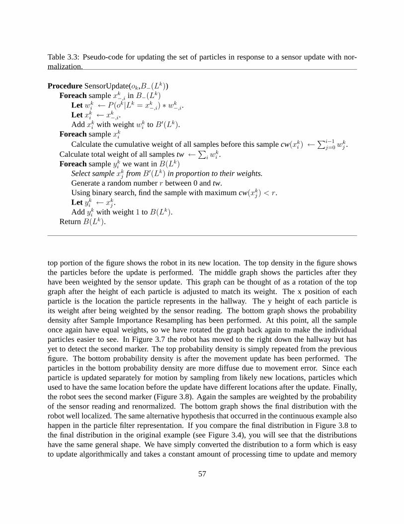
Table 3.3: Pseudo-code for updating the set of particles in response to a sensor update with nor-malization.

ProcedureSensorUpdate(ok,B−(Lk))Foreachsamplexk

−,i in B−(Lk)Let wk

i ← P (ok|Lk = xk−,i) ∗ wk

−,i.Let xk

i ← xk−,i.

Add xki with weightwk

i to B′(Lk).Foreachsamplexk

i

Calculate the cumulative weight of all samples before this samplecw(xki ) ←

∑i−1j=0 wk

j .Calculate total weight of all samplestw ←

∑i w

ki .

Foreachsampleyki we want inB(Lk)

Select samplexkj fromB′(Lk) in proportion to their weights.

Generate a random numberr between 0 andtw.Using binary search, find the sample with maximumcw(xk

j ) < r.Let yk

i ← xkj .

Add yki with weight1 to B(Lk).

ReturnB(Lk).

top portion of the figure shows the robot in its new location. The top density in the figure showsthe particles before the update is performed. The middle graph shows the particles after theyhave been weighted by the sensor update. This graph can be thought of as a rotation of the topgraph after the height of each particle is adjusted to match its weight. The x position of eachparticle is the location the particle represents in the hallway. The y height of each particle isits weight after being weighted by the sensor reading. The bottom graph shows the probabilitydensity after Sample Importance Resampling has been performed. At this point, all the sampleonce again have equal weights, so we have rotated the graph back again to make the individualparticles easier to see. In Figure 3.7 the robot has moved to the right down the hallway but hasyet to detect the second marker. The top probability density is simply repeated from the previousfigure. The bottom probability density is after the movement update has been performed. Theparticles in the bottom probability density are more diffuse due to movement error. Since eachparticle is updated separately for motion by sampling from likely new locations, particles whichused to have the same location before the update have different locations after the update. Finally,the robot sees the second marker (Figure 3.8). Again the samples are weighted by the probabilityof the sensor reading and renormalized. The bottom graph shows the final distribution with therobot well localized. The same alternative hypothesis that occurred in the continuous example alsohappen in the particle filter representation. If you compare the final distribution in Figure 3.8 tothe final distribution in the original example (see Figure 3.4), you will see that the distributionshave the same general shape. We have simply converted the distribution to a form which is easyto update algorithmically and takes a constant amount of processing time to update and memory

57

space to store.

Now that we can track a belief state about the robot’s pose, we need to get this information tobehaviors in a useful form. Behaviors are interested in knowing the most likely pose of the robot.We can approximate this by calculating the mean pose of the robot. Each position coordinate ofthis mean pose can be calculated independently from the particle set as a simple weighted average.

x =

∑i xi.x ∗ wi∑

i wi

In this formula,xi.x is used to indicate the x coordinate of particlexi. The heading of this meanpose can be calculated using a weighted average over heading vectors computed from each particle.

Behaviors also need a way to judge the reliability of the estimate. The covariance matrix providesa convenient way to summarize the uncertainty in the result. This reports the variance in eachcoordinate and their correlation. The covariance matrix can be easily calculated from the particlesusing the standard statistics formulas. This information can be used to actively trigger behaviorsto gather information useful for localization amongst other uses.

For a more complete description of Monte Carlo Localization, please see Fox et al. [16] and Del-laert et al. [11].

58

Figure 3.5: Robot starts off lost. See text for explanation.

Figure 3.6: Robot sees a marker to its side. The first density is before the update and the last isafter the update. See text for explanation.

59

Figure 3.7: Robot continues moving to right. The first density is before the update and the last isafter the update. See text for explanation.

Figure 3.8: Robot sees another marker to its side. The first density is before the update and the lastis after the update. See text for explanation.

60

3.4 Limitations of Monte Carlo Localization

For certain robots, MCL provides a robust solution to the localization problem. The robot musthave sufficient computational power to process a large number of samples. A large number ofsamples is needed in order to represent the belief state with sufficient resolution. An accurateand complete model of the movement of the robot when different motion commands are executedmust be available. An accurate and complete model of the values that sensors can return mustbe available. Unfortunately, for many robots these conditions are not met. In particular, in theRoboCup domain in which we tested, none of these conditions are met. The algorithm may fail fora number of reasons: inaccurate models of movement and sensor noise, external disturbance of therobot’s location, or insufficient sample count to accurately approximate the probability density.

Accurate and complete motion models for the robot are not available. Due to the nature of leggedlocomotion, significant errors in odometry occur as the robot moves about. These errors are diffi-cult to model because they depend on the dynamics of the robot, the previous state of the robot’sjoints, and the particular properties of the flooring the robot is currently walking on. For instance,a slight tilt in the floor can result in a significant arc in the motion of the robot when it is simplytrying to move straight forward. Further noise is introduced into odometry readings by frequentextended collisions with the walls and other robots. Since we are unable to detect collisions andare unable to locate other robots, we cannot model collisions with other robots introducing error inour system. An additional complication is introduced by the rules which specify that under certaincircumstances the robot is to be moved by the referee without telling the robot. Even if we couldmodel all of these events, the cost in development time to develop all of these models would beprohibitively expensive. Even worse, none of these models would be useful on a different robot orin a different environment.

MCL is only capable of handling small systematic errors in movement. Every sensor reading givesMCL a chance to correct a small amount of systematic error. The amount of systematic error thatcan be corrected for increases with larger movement deviations and larger numbers of samples. Ifthe systematic error in movement gets too large, MCL will slowly accumulate more and more error.We need to handle systematic errors in movement because measuring the movement parametersfor a robot is time consuming and error prone. Systematic errors in movement also occur whenthe environment changes in unmodeled ways. For example, if the robot moves from carpeting toa plastic surface such as the goal, the movement of the robot for the same motion commands islikely to change.

MCL does not handle unexpected/unmodeled robot movements very well. The time MCL takesto recover is proportional to the magnitude of the unexpected movement. During this time, MCLreports incorrect locations. Unexpected movements happen frequently in the robot soccer domainwe are working in. Collisions with other robots and the walls result in motions having unexpectedresults. Collisions are difficult to detect on our robots and thus cannot be modelled by the localiza-tion algorithm. Another unexpected movement we incur is teleportation due to application of therules by the referee. MCL takes a long time to recover from this.

61

Accurate and complete sensor models for the robot are unavailable. Sensor readings are often bi-ased in different ways depending on the location of the robot. So, one location may consistentlygive distance readings that are too low while another location may consistently give distance read-ings that are too high. We have to ignore this dependence because it is too expensive to try tocalibrate the distance readings at every possible location the robot might be at and the distancereadings often depend on lighting conditions which can potentially change frequently. This sys-tematic bias violates the independence assumption used to derive the localization algorithm leadingto inevitable errors in localization.

In addition to the problems with inaccurate and incomplete models, for many situations the numberof samples that can be processed is fewer than are needed due to processing constraints. Globallocalization is the process of determining the robot’s location from an initially unknown location.More samples are normally needed by Monte Carlo Localization during global localization thanwhen tracking since similar resolution is needed and the samples are spread over a much largerarea. If MCL is run with too few samples during global localization, the locale probability densityprematurely collapses to the few most likely points. With only 400 samples (to keep computationalload low) there is only 1 sample for every100cm2 ignoring orientation for the moment. Duringtesting with 1000 samples, we commonly observed the sample set collapse to 1–2 distinct samplesduring global localization from a single marker observance. Thus, the probability density collapsesto very small number of samples from the infinitely many locations that are consistent with a singlemarker observance. The number of samples remains constant, of course, but the number of distinctsamples is often reduced greatly during the sensor update phase. A single marker reading localizesthe robot to a circle around the marker at a set distance and a heading relative to the center ofthe circle. Obviously, 1-2 distinct samples are not sufficient to represent this circle accurately.Adaptive sample set sizes do not help much here since only one movement update step is resampledfrom. If the robot takes 2 steps and then sees a marker, the probability density will consist of 1-2tightly grouped blobs instead of 1-2 points which doesn’t fix the problem. The premature collapseof the probability density results in increased time for global localization and more misleading errorin position during global localization. Since our robots are continually losing track of their positiondue to collisions, being moved, falling down, etc., it is extremely important that the localizationalgorithm be capable of globally localizing quickly.

Some of the drawbacks of MCL can be alleviated somewhat by adding adaptive sample set sizing.Even with adaptive sample set sizing, MCL is still sensitive to systematic errors in movement.MCL with adaptive sample set sizing requires different computational resources as the number ofsamples changes. Adaptive sample set sizing as described in Fox et al. [16] can take an extremelylong time if the robot thinks it is one position and the sensor readings indicate a different position,especially if robot movements are very accurate. We were unable to apply MCL with adaptivesample set sizing since we are working in a real time domain and do not have any additionalcomputational power available.

A later approach to alleviating the drawbacks of MCL was introduced in 2000 by Thrun and Foxafter this work was completed [57]. In this approach, called Mixture-MCL, in addition to updatingsamples for movement and weighting by sensor readings, samples are also generated by sensor

62

readings and weighted by the motion model. This modification to the sample generation results ina better approximation to the probability density predicted by the model and helps reduce the num-ber of samples needed at the expense of more computation per sample used. Unfortunately, thisdoes nothing to directly correct for errors that might be present in the model. This new samplingprocedure recovers from a teleportation faster than normal MCL does, but the recovery rate is stillconstrained by the motion model. A motion model with little error coupled with a observationmodel with a much larger relative error will still result in a slow convergence rate to the correctposition after the robot is teleported.

In many ways, Mixture-MCL is a complementary approach. Mixture-MCL reduces the chancethat the probability density will fail to converge to the correct solution and Sensor Resetting Lo-calization decreases the time to recover from a failure.

3.5 Sensor Resetting Localization

Sensor Resetting Localization (SRL) is an extension of Monte Carlo Localization [17] based onthe principle of change detection for failure recovery. The key idea behind SRL is to monitorthe likelihood of the sensor readings given the current estimate of the robot’s position. Failuresin localization can be detected by monitoring for operating environment changes reflected in thissignal. By monitoring this likelihood, the algorithm detects a phase transition between globallocalization (localization from an unknown position) and tracking (updating position estimates asthe robot moves and senses). The algorithm also detects a phase transition between algorithmfailure (due to insufficient representative power of the probability distribution) and tracking. Bydetecting these phase transitions, the algorithm is able to adapt by temporarily weighting the sensorreadings more heavily than usual. This adaptation is a failure recovery action that allows for quickrecovery.

SRL uses the same particle filter representation for the robot’s belief state as used in MCL. SRL isheavily based on the MCL algorithm and readers are encouraged to read Section 3.2 and Section 3.3before reading this section as concepts and procedures introduced in those sections are elided hereto avoid repetition.

SRL is motivated by the desire to use fewer samples, handle larger errors in modelling, and handleunmodeled movements. SRL adds a new step, called sensor resetting, to the sensor update phaseof the algorithm. If the probability of the sensor readings is low given the position designated bythe samplesP (ok|Lk), we replace some samples with samples drawn from the probability densitygiven by the sensorsP (Lk|ok). The number of samples kept is proportional to the average prob-ability of a locale sample given the sensors divided by an expected average probability of localesamples. Thus if the average probability is above a threshold, all the samples are kept. As theaverage probability of the locale samples falls below this threshold, more and more samples arereplaced by samples based on the sensor readingsP (Lk|ok). We call this sensor based resampling.The logic behind this step is that the average probability of a locale sample is approximately pro-portional to the probability that the locale sample set covers the actual location of the robot, i.e.

63

Table 3.4: Pseudo-code for SRL for updating the set of particles in response to a sensor update.

ProcedureSensorUpdate(ok,B−(Lk))Foreachsamplexk

−,i in B−(Lk)Let wk

i ← P (ok|Lk = xk−,i) ∗ wk

−,i.Let xk

i ← xk−,i.

Add xki with weightwk

i to B′(Lk).Foreachsamplexk

i

Calculate the cumulative weight of all samples before this samplecw(xki ) ←

∑i−1j=0 wk

j .Calculate total weight of all samplestw ←

∑i w

ki .

Foreachsampleyki we want inB(Lk)

Select samplexkj fromB′(Lk) in proportion to their weights.

Generate a random numberr between 0 andtw.Using binary search, find the sample with maximumcw(xk

j ) < r.Let yk

i ← xkj .

Add yki with weight1 to B(Lk).

Calculate number of new samples to generate.Let ns ← (1− tw/prob threshold) ∗ num samplesIf (ns> 0) repeatnstimes

Draw sample(s′) from P (L|ok).Replace a random sample fromB(Lk) with s′.

ReturnB(Lk).

the probability that we are where we think we are. Taking one minus this value as the probabilityof being wrong, suggests that we should replace a proportion of samples equal to the probabilityof being wrong with samples from the sensors. The constant of proportionality between the aver-age probability of a locale sample and the probability of being wrong is a parameter that can betweaked to control how often the localization algorithm resets itself.

The SRL algorithm consists of a motion update procedure and a sensor update procedure. The mo-tion update procedure is exactly the same as in MCL (see Table 3.1). The sensor update procedureis the same as in MCL except that an additional sensor resetting step is added. This step checks forthe failure of the algorithm and executes a recovery action if necessary. This procedure is shownin pseudo-code in Table 3.4.

3.6 Sensor Resetting Localization Discussion

The goal of sensor based resetting is to return the probability density to a sane state wheneverit appears that the algorithm may be failing. Here, a sane state means one that reflects all likely

64

−2000 −1500 −1000 −500 0 500 1000 1500 2000

−1000

−800

−600

−400

−200

0

200

400

600

800

1000

x position (mm)

y po

sitio

n (m

m)

−2000 −1500 −1000 −500 0 500 1000 1500 2000

−1000

−800

−600

−400

−200

0

200

400

600

800

1000

x position (mm)

y po

sitio

n (m

m)

−2000 −1500 −1000 −500 0 500 1000 1500 2000

−1000

−800

−600

−400

−200

0

200

400

600

800

1000

x position (mm)

y po

sitio

n (m

m)

Figure 3.9: The sequence of belief states resulting from a robot in an unknown initial locationseeing one landmark.

locations of the robot. The algorithm may fail for a number of reasons: inaccurate models ofmovement and sensor noise, external disturbance of the robot’s location, or insufficient samplecount to accurately approximate the probability density. We restore the probability density to asane state by replacing the density with one consistent with the robot’s current sensor readings andthe robot’s prior belief of likely locations to be located on the field (we use a uniform distributionfor this). We apply this resetting step any time we find that our belief state is inconsistent with thecurrent sensor readings. Inconsistency can be measured by using the sensor probability model toestimate the likelihood of the sensor readings given our current belief state. See Figure 3.9(right)for an example of the result of a reset event. Without this step, the algorithm is the same as thepopular Monte Carlo Localization technique [17].

This sensor resetting step was added to solve a problem recovering the robot’s location from aninitially unknown location (see Figure 3.9 left). With only 400 samples (to keep computationalload low) there is only 1 sample for every100cm2 and even less are available after accounting fororientation. Usually only 1–4 of the 400 samples are consistent with a single landmark observationobservation (see Figure 3.9 middle). Resetting solves this problem by concentrating the samplesin locations that are consistent with the landmark observation (Figure 3.9 right) providing a muchbetter approximation of the infinitely many locations that are consistent with this marker reading.Adding sensor based resetting also solved several other problems. By resetting, we automaticallyrecover from errors in the movement model and external disturbances. External disturbances arecaused by the referee moving the robot or collisions with other robots.

Sensor Resetting Localization is applicable in domains where it is possible to sample from thesensor readingsP (L|o). This sample generation is not a problem if landmarks are being usedas the sensor readings as the sensor distributions are easy to sample from. However, this samplegeneration can be difficult to do for sensor readings that entail complex distributions. If all possiblelocations of the robot are known, this sensor based sampling can be done by rejection sampling.However, rejection sampling increases the run time for resampling in proportion to the probabilityof having to reject a sample. Other general sampling techniques such as Monte Carlo MarkovChain techniques can be applied here to generate samples in accordance with arbitrary probabilitydensities, however, efficiency may be a concern depending on the precise form of the probabilitydensity implied by the sensor readings.

65

One of the advantages of SRL is that fewer samples can be used without sacrificing much accuracy.This is possible in part because it is more efficient when globally localizing. When the first markeris seen during global localization, the probability of almost all of the samples is very low. Thusthe average probability of a sample is ridiculously small and SRL replaces almost all the locationsamples with samples from the sensors. This results in all of the samples being distributed evenlyaround the circle determined by the marker. So, if we are using 400 samples, we have 400 sam-ples instead of the 1–2 of MCL to represent the circle around the marker. Naturally, this reducesmisleading errors during global localization. This also reduces the time required to converge tothe correct localization since the correct answer has not been thrown out prematurely. After see-ing another marker the circle collapses to a small area where the circles intersect. The averageprobability of the locale samples now is much higher than after seeing the first marker since moresamples have been concentrated in the right place by the first sensor reading. Thus, if the thresholdfor sensor based resampling is set correctly, no new samples will be drawn due to the second sensorreadings. As long as tracking is working, no new samples are generated from the sensors and thealgorithm behaves exactly like MCL.

SRL can handle larger systematic errors in movement because once enough error has accumulated,SRL will replace the current estimate of the robot’s location with one based on the sensor readings,effectively resetting the localization. Adaptive sample set sizing helps MCL, but MCL is still moresensitive to systematic errors in movement and unexpected/unmodeled robot movements. SRL isalso easier to apply to real time domains since the running time per step is nearly constant and easyto bound.

SRL can handle larger unmodeled movements than MCL. The localization algorithm needs tohandle extended collisions with other robots and the wall gracefully. SRL does this by resettingitself if its estimate of current robot position gets too far off from the sensor readings. SRL is ableto handle large unmodeled movements such as movement by the referee easily. SRL does this byresetting itself the first time it gets a sensor reading that conflicts with its estimated position. MCLwould take a long time to correct for long distance teleportation such as this since enough error inmovement has to occur to move the mean of the samples to the new location.

In summary, Sensor Resetting Localization offers the following benefits:

• Sensor based resetting allows for poorer approximations and models to be used.

• Sensor based resetting provides fault tolerance and failure recovery in the robot localization.

• Sensor Resetting Localization is robust to external disturbances.

3.7 Environment

Sensor Resetting Localization was developed for use in the Sony legged league of the robot soccercompetition RoboCup ’99. The algorithm has been tested in this domain, in separate tests with the

66

same hardware and environment, and in simulation. These tests used an older version of the robotand RoboCup field than those described in the background chapter. The basics about the robot,software, and field used in these tests is described in this section. We also describe some of thefeatures of this domain make the localization problem especially challenging.

Hardware The robots used in the competition and tests were generously provided by Sony [19].These robots are the AIBO ERS-110 model robots developed by Sony. The robots are a excellentplatform for research and development and provide us exceptional hardware that is commerciallyviable. The robot consists of a quadruped designed to look like a small dog. The robot is approxi-mately 20cm long plus another 10cm due to the head. The neck and four legs each have 3 degreesof freedom. The neck can pan almost90◦ to each side, allowing the robot to scan around the fieldfor markers. The robot stands 20cm high at the shoulder with the head extending another 10cm.

Vision Vision is provided by a color CCD camera with a resolution of 88x60. The robot’s field ofview is about60◦ horizontally and40◦ vertically. The input from the camera is processed by colorseparation hardware and analyzed by the vision system to return distance and angle to any markersseen. Distance is estimated based on distance between color blob centers. Distance estimates varyby about±15% when the robot is standing still. The mean value is usually within about 10% fordistance and7◦ for angle. Markers which are partially off of the camera look like noise to the visionsystem. The sides and edges of markers are commonly missed by the vision system. Because ofthese effects, sensor readings occasionally have much larger errors than usual. The vision systemsubtracts out the neck angle before passing the result to the localization algorithm. The neck angleis sensed using an on-board sensor that is very accurate but has a high granularity. These markerdetections with distance and angle provide the sensor readings used to perform sensor updates forlocalization.

Locomotion The locomotion used in all our tests was developed by Sony. Due to the complex-ities of legged locomotion, there is a lot of variability in the motion performed by the robot forthe same motion commands. Repeatedly executing a path of approximately 5m in length with twoturns results in final positions of the robot that vary by about 1m. As the robot moves, its feet sliprandomly on the surface of the field contributing to the large movement error. The robot can tran-sition among different types of motion such as forward, forwardright, right forward, turnright,backward, etc., each in different gaits. The robot slips randomly on the field surface when transi-tioning from one motion to another. Slippage from transitions can be as much as5◦ but does nottend to affectx,y position much. Additional errors in movement are introduced by different resultsfor the same robot behavior under slight changes to the environment such as slightly different fieldsurface or somewhat lower battery charge. These day to day variations in robot behavior are tooexpensive to model because of the time it takes to determine model parameters. Systematic errorsof up to 25% have been observed in our lab.

67

The Field The field on which the robot operates is 2.8m in length by 1.8m in width. The fieldis surrounded by low sloped walls that keep the robots and the ball on the field. There is a colorcoded goal at each end of the field, one cyan and one yellow, that were not used as input to thelocalization. The surface of the field is a short carpeting except in the goals where the surface is asmooth plastic.

The field is surrounded by 6 markers, 3 on each of the long sides of the field. There is a marker ineach corner, and one at each end of the center line. Each marker is a color coded cylinder mounted20cm from the surface of the field which is about eye level to the robot. Each cylinder is 20cm highand 10cm in diameter. The cylinder is divided vertically into two equal sized colored patches, onepink and either cyan, green, or yellow to indicate position along the long axis of the field (whichwe refer to as thex axis). Whether the pink is on the top or bottom indicates which side of thefield the marker is on. Thus, there are 6 uniquely distinguishable markers to which the robot canestimate distance and angle.

Challenges The Sony legged league of the robot soccer competition RoboCup ’99 provides achallenging domain in which to do localization. Due to the nature of legged locomotion, significanterrors in odometry occur as the robot moves about. Further noise is introduced into odometryreadings by frequent extended collisions with the walls and other robots. Since we are unableto detect collisions and are unable to locate other robots, we cannot model collisions with otherrobots introducing error in our system. Noise in the vision processing also makes localization moredifficult. An additional complication is introduced by the rules which specify that under certaincircumstances the robot is to be moved by the referee without telling the robot. The followingchallenges must be addressed by the localization system:

• Errors(occasionally large) in sensor readings

• Systematic errors in sensor readings

• Large amounts of noise in odometry

• Systematic errors in odometry

• Collision induced unmodeled movements

• Referee induced large unmodeled movements

3.8 Implementation Details

This section describes implementation details of the localization used in testing. Unless other-wise noted, all implementation details are the same between Monte Carlo Localization and SensorResetting Localization.

68

The particle locations are represented as an array ofn locations on the soccer field. High particlecounts tend to result in better accuracy and robustness at the cost of additional computation. Weusedn = 400 particles in our system as a reasonable compromise. There are three basic typesof updates we perform on the sample set: movement updates, sensor updates, and sensor basedresetting. The basic update cycle is: move robot, update for movement, read sensors, update forsensors, reset if necessary, repeat. The mean of the samples is taken to be the best estimate for thelocation of the robot and the standard deviation of the samples is used to estimate the uncertainty.

We modeled all of our movements by 3 Gaussians, one for movement distance, one for movementdirection, and one for heading change. We represented our sensor distributions as 2 Gaussians,one for distance from the landmark and one for egocentric angle to the landmark. We set deviationequal to a percentage of the mean for distance and a constant value for angle.

We attempted to do one sensor update stage for each movement update stage. However, we discov-ered that even when using only 400 samples the localization algorithm was too slow. To make thealgorithm real time, we ignored sensor readings whenever the localization algorithm fell behind onmovement updates. When throwing away sensor readings, we were able to execute about twice asfast but sacrificed a small amount of accuracy and a large amount of precision.

For Sensor Resetting Localization, we used a sensor based resampling threshold equal to the ex-pected result of 20% of the samples being distributed according to the sensor Gaussians and theother 80% having probability 0.

3.9 Results

We tested Sensor Resetting Localization on the robots provided by Sony and in simulation. Insimulation testing, we also compared Sensor Resetting Localization with Monte Carlo Localizationwith and without random noise samples added.

We tested SRL on the real robots using the parameters we used at RoboCup ’99. We used 400samples for all tests. In order to execute in real time, we were forced to ignore about 50% of thesensor readings. Due to inevitable changes in conditions between measuring model parametersand using them, the parameter for distance moved was off≈ 25%, for angle of movement≈ 10◦,and for amount of rotation≈ .6◦/step. The deviations reported to the localization were 10% formovement and 15% for vision. We had the test robot run through a set trajectory of 156 stepswhile slowly turning it neck from side to side. The robot was instructed to stop after 7 differentnumbers of steps had been executed. The final position of the robot was measured by hand foreach run. We did five runs at each of the 7 number of steps and averaged the results. We comparedthe actual location of the robot at each of the 35 data points with the location reported by thelocalization algorithm. We calculated the error in the mean position over time and the deviationthe localization reported over time. We also calculated an interval in each dimension by taking themean reported by the localization and adding/subtracting 2 standard deviations as reported by thelocalization. We then calculated the distance from this interval in each dimension which we refer

69

x (mm) y (mm) theta (◦)

average error 99.94 95.14 14.29average interval error 15.18 4.91 2.07

rms interval error 34.92 13.94 3.82in box percentage 74.29% 80.00% 57.14%

Table 3.5: Performance summary on real robots.

to as interval error. We report both average interval error and root mean squared interval error. Wefeel that root mean squared interval is a more appropriate measure since it weights larger, moremisleading errors more heavily. We also calculated the percentage of time that the actual locationof the robot fell within the 3D box defined by thex,y, andθ intervals.

Table 3.5 shows the localization is accurate within about 10cm inx andy and15◦ in θ despitethe erroneous parameter values. The actual location of the robot is within the box most of thetime and when it is outside the box, it is close to the box. The fact that the localization seldomgives misleading information is very important for making effective behaviors. Figure 3.10 showthat the error in position quickly converges to a steady level. Figure 3.11 shows that the deviationreported by the algorithm quickly converges to a fairly steady level. The deviation tends to go upat the same time the error goes up which keeps the interval error low and avoids misleading output.In competition, we observed that the localization algorithm quickly resets itself when unmodelederrors such as being picked up occur.

In simulation, we tested Sensor Resetting Localization against Monte Carlo Localization with andwithout random noise. Since the developers of Monte Carlo Localization suggested adding a fewrandom samples to help the algorithm recover from errors, we tested Monte Carlo Localizationadding no random noise samples and adding 5% random noise samples. Each test was run 30times and the results averaged. All tests were run with 400 samples unless otherwise noted. Thesimulator models the movement of the robot with the same probability density used by the local-ization algorithm. Each step the probability density for motion is sampled once to generate thenew position of the robot. The parameters for the movement model are the same parameters weused in RoboCup ’99. The robot’s vision system is modelled by assuming that the vision systemcorrectly identifies everything within the robot’s view cone and estimates the correct distance andangle to each marker. The reported deviation on the vision information as given to the localizationalgorithm is 15%. We modelled the movement of the robot’s neck in the simulator by having itsweep through a set of degrees relative to the body at the same pace that the real robot used. Theneck movement allowed the robot to see many different markers from almost all field positions.

Figure 3.12 shows that SRL has less error than MCL localization with small sample sets. Fig-ures 3.12 and 3.13 show the mean error and 95% confidence interval error bands. Once the sampleset has increased to about 5000 samples, the two algorithms give almost identical performance.Since performance of MCL with noise samples was slightly worse than MCL without noise sam-ples, especially at small sample sizes, MCL with noise is not shown in these figures. Interestingly,

70

0 20 40 60 80 100 120 140 1600

100

200

300

400

500

600

700

steps taken

x pos

ition

erro

r (m

m)

SRL on real robots (mean)

Figure 3.10: Error on real robots versus time.

0 20 40 60 80 100 120 140 1600

100

200

300

400

500

600

700

steps taken

x pos

ition

devia

tion

(mm

)

SRL on real robots (mean)

Figure 3.11: Deviation reported by localization on real robots versus time.

71

101

102

103

104

105

20

40

60

80

100

120

140

160

180

200

220

# of samples

x pos

ition

erro

r (m

m)

SRL (mean + error bands)MCL without noise (mean + error bands)

Figure 3.12: Simulation error versus number of samples.

the error of SRL stayed about constant above 100 samples was usable with only 10 samples. Fig-ure 3.13 shows that SRL gives fewer misleading results than MCL. SRL gives fewer misleadingresults even at intermediate sample counts where the error between SRL and MCL has almostdisappeared.

Figures 3.14 and 3.15 show that SRL is able to do global localization quicker than MCL using 400samples. The figures show mean error and two standard deviations from the mean (the deviationlines arenoterror bars). SRL is able to globally localize in about 10 steps whereas MCL takes about60 steps. In noisy domains with adversarial robots, we can’t afford to spend 60 steps localizing.The global localization performed by SRL is more consistent than MCL making its output easierto reason with. Surprisingly, adding noise to MCL hurts global localization. We noticed in testingthat MCL with noise pays a penalty in larger deviations than the other two algorithms. Figure 3.16shows the average interval error over time for the 3 algorithms (see the experiment on real robotsabove for a description of interval error). Unlike SRL, MCL generates large interval errors duringglobal localization which indicates that it is producing very misleading outputs.

We also tested the response of SRL and MCL to systematic errors in movement and vision. Wesimulated systematic movement errors by multiplying the actual distance the robot moved andturned in the simulator by a constant factor between 0.1 and 1.9 without telling the localizationalgorithm. This shows the sensitivity of the algorithm to movement parameters which is importantwhen movement parameters are expensive or difficult to measure. We also simulated systematicerror in vision by multiplying all distance estimates passed to the localization by a constant factor

72

101

102

103

104

105

0

20

40

60

80

100

120

140

160

180

200

220

# of samples

x pos

ition i

nterva

l erro

r (mm

)

SRL (rms + error bands)MCL without noise (rms + error bands)

Figure 3.13: Simulation interval error versus number of samples.

0 10 20 30 40 50 60

−200

0

200

400

600

800

steps taken

x pos

ition

erro

r (m

m)

SRL (rms ± 2 standard deviations)MCL with noise (rms ± 2 standard deviations)

Figure 3.14: Simulation SRL and MCL with noise error versus time.

73

0 10 20 30 40 50 60

−200

0

200

400

600

800

steps taken

x pos

ition

erro

r (m

m)

SRL (rms ± 2 standard deviations)MCL without noise (rms ± 2 standard deviations)

Figure 3.15: Simulation SRL and MCL without noise error versus time.

0 20 40 60 80 100 120 140 1600

50

100

150

200

250

300

steps taken

y pos

ition

inter

val e

rror (

mm

)

SRL (rms)MCL without noise (rms) MCL with noise (rms)

Figure 3.16: Simulation SRL and MCL interval error versus time.

74

0 0.5 1 1.5 20

100

200

300

400

500

600

700

systematic movement error

y po

sitio

n er

ror (

mm

)SRL (mean + error bands)MCL with noise (mean + error bands)

0 0.5 1 1.5 20

100

200

300

400

500

600

700

systematic movement error

y po

sitio

n er

ror (

mm

)

SRL (mean + error bands)MCL without noise (mean + error bands)

0.6 0.8 1 1.2 1.4 1.6 1.80

50

100

150

200

250

300

350

400

450

500

systematic vision error

y po

sitio

n er

ror (

mm

)

SRL (mean + error bands)MCL with noise (mean + error bands)

0.6 0.8 1 1.2 1.4 1.6 1.8 20

50

100

150

200

250

300

350

400

450

systematic vision error

y po

sitio

n er

ror (

mm

)

SRL (mean + error bands)MCL without noise (mean + error bands)

Figure 3.17: Simulation SRL and MCL error versus systematic model error.

between 0.7 and 1.75. Figure 3.17 shows that SRL is more robust to modelling error than MCLespecially in regards to systematic movement error. Shown in the figures is the mean and 95%confidence interval error bands.

There is a tradeoff between robustness to systematic movement error and systematic vision error.SRL and MCL with noise favor robustness to movement errors while MCL without noise favorsrobustness to vision errors. MCL without noise performs better than SRL for large systematicvision errors. SRL performs better than MCL with noise in all cases with similar response tovision errors and lower errors when presented with movement errors. SRL is much more robust toerrors in movement than MCL without noise, especially when the movement error is larger than afew standard deviations.

3.10 Conclusion

Sensor Resetting Localization(SRL) provides an effective localization option for real time sys-tems with limited computational resources. The technique is applicable in Markovian domainswhere locale samples can be drawn from the sensor readings, i.e. it must be possible to samplefrom P (L|o). SRL requires a constant amount of processing power unlike Monte Carlo Localiza-

75

tion(MCL) with adaptive sample set sizes which attempt to address some of the same issues asSRL. SRL achieves better results than MCL using small sample sets, which translates into smallercomputational resource requirements. SRL is able to localize effectively using very small samplesets and very little computational power. Part of the reason SRL is able to accomplish this is SRL’sability to globally localize using fewer samples. SRL automatically resets itself before errors canaccumulate too much allowing it to gracefully recover from errors in modelling such as collisionsand teleportation. SRL is less sensitive than MCL to systematic errors in modelling except for largeerrors in vision when using MCL without random noise samples added. SRL is particularly robustwith respect to systematic errors in movement. In addition to these benefits, the algorithm almostnever returns misleading information. The algorithm correctly reports the reliability of its bestguess of the location of the robot. Sensor Resetting Localization is an accurate, easy to use tech-nique that is able to perform robust localization with very small computational resources. Thesebenefits are due to the ability of SRL to determine the state of its own performance (or the cur-rent operating conditions or environment for the localization) and adapt using that information. Amore recent comparison of localization techniques including SRL was created by Guttmann [22].The best performing localization in the test was Adaptive-MCL(A-MCL) which is a derivative ofSRL which improves upon the detection of phase transitions in the performance of the algorithm.These localization techniques can occasionally fail due to lack of resolution in the approximationof the probability density representing the robot’s location or inaccurate models. SRL pioneeredaddressing the problem of failure of the localization algorithm. As shown by the performance ofSRL and A-MCL in this evaluation, this work continues to show its value.

Applying the concept of environment identification for failure recovery to localization results ina more robust localization algorithm. This improvement motivates the further investigation of thepower of environment identification for improving robot performance. As shown by A-MCL, amore robust identification of the operating environment (and accompanying environment transi-tions) leads to even better performance. The desire for a robust, general method for environmentidentification leads to the development of the algorithms in the next chapters.

3.11 Summary

In this chapter, we applied the concept of environment identification for failure detection and re-covery to the problem of localization. We explained how localization algorithms work in generaland how particle filters work in particular. We modified a popular particle filter approach to lo-calization to include the concept of environment identification for failure recovery. We showedthrough extensive testing, that using environment identification results in a more robust algorithmwith lower computational requirements.

76

Chapter 4

Environment Identification in Vision

In this chapter, we continue our exploration in environment identification, this time in the contextof vision. We develop a more general on-line algorithm for environment identification that is basedon learning about the environments from training data. We use this algorithm to adapt to changinglighting conditions to improve performance of our color-based vision. We show that the algorithmleads to improved performance in a relatively simplistic task. Finally, we discuss the shortcomingsof this approach which we rectify in the algorithms presented in the following chapters.

4.1 Introduction

It is important that robots be able to identify the current operating environment. Without thisability, the robot is unable to use information that has been acquired previously about the currentenvironment (through instruction or learning) to improve its behavior. While the robot may beable to re-adapt to the revisited environment, this will almost certainly take longer than identifyingthat the environment has re-occurred. Identifying the current environment (which may depend onthe state of other agents) allows the robot to adapt to the behaviors of other agents by recognizingrepetition in their actions.

In the trivial case, the current environment can be determined from a single observation. Thiscase is not very interesting and is handled well by current techniques. In many systems, however,a single observation contains very little information about the current environment. Even all ofthe observations at a single point in time are likely to be insufficient to determine the currentenvironment. This is usually due to each individual sensor reading providing only a small partof the information and/or being subject to large levels of noise. For instance, a single pixel froma camera image (or range from laser range finder/sonar) gives very little information about thestate of the world. A complete image (or range scan) provides a treasure trove of information ifit can only be extracted. Both of these problems can be overcome by aggregating the individualsensor readings into probability distributions (over time or space). These probability distributions

77

Figure 4.1: Robot used in testing.

must then be compared to detect similar distributions if repeated environments are to be identified.Since the robot should generalize over nearby environments when possible, it is not enough tosimply use statistical tests to determine similarity. This is due to the nature of statistical tests inmerely determining different/same rather than giving an indication of the degree of difference thuspreventing the robot from identifying nearby environments.

Other researchers have also looked for ways to identify environments from windows of sensor sig-nals. Like the approach described in this chapter, these approaches suffer from limitation imposedby the use of windows. These limitations include inherit latency, ambiguous labelings for windowswhich span across a transition point, and difficulty incorporating transition frequency information.These other techniques are described and discussed in more detail in the related work chapter,Chapter 7. Examples of other window based approached include those of Chen et al. [9] and Caoet al. [7] amongst many others.

We applied this thinking to the problem of adapting to changing lighting conditions. The robotused in this work is the commercially available AIBO ERS-210 robot built by Sony. The robot is

78

pictured in Figure 4.1. Many practical color robotic vision systems rely on consistent pixel read-ings that allow colors to be segmented without reference to the surrounding pixel context. We usethe free CMVision vision system to perform image processing [6, 5]. The vision algorithms usedby CMVision are also described in the background chapter (Chapter 2) in Section 2.5. Since actualpixel readings vary with lighting conditions and the separation between colors is often small, thesesystems are highly dependent on consistent lighting conditions. Changing the lighting conditionsinvolves recalibrating the vision system for the new conditions. We propose a solution to this prob-lem which automatically detects the current lighting conditions and switches to a correspondinghuman or machine supplied calibration.

We begin by describing the algorithm for segmenting the data into different environments in Sec-tion 4.2. In Section 4.3, we describe the algorithm we use for converting segmented data into classlabels that identify the current environment. We describe how this knowledge is used to improvethe performance of robotic vision by adapting to the current environment in Section 4.4. We alsodescribe testing procedures and results in this section. We finish with a discussion of the limitationsof the algorithm and our conclusions in Sections 4.5 and 4.6, respectively.

4.2 Algorithm

In order to understand the on-line algorithm, it helps to start by considering the off-line version.The basic problem is to identify the current lighting conditions from data summarizing what thecamera is seeing. It is desirable to use a small amount of information to summarize the overalllighting of the scene captured by the camera to reduce memory and computation requirements.Simply using the average luminance (or brightness) of the scene is sufficient for separation andeconomical in representation. Of course, the average luminance of a scene depends highly onwhat is being looked at. Therefore, instead of relying on a single measure of average luminance,a distribution of luminance values over the recent past is considered. The basic problem thenbecomes to segment the time series of average luminance values into distinct regimes (or regions)which have similar distributions of average luminance measurements.

Having decided to look for similar distributions of measurements, it is now necessary to have a wayto determine whether two distributions are in fact the same distribution and how similar they are.Since the shape and form of the distribution is unknown, a non-parametric distance metric is used.The particular distance metric used affects the decisions of the clustering algorithm. The distancemetric controls the bias of the learning algorithm. Note that statistical difference tests such as theKuiper test [32] or Kolmogrov-Smirnov test are inappropriate as they measure the probability ofdifference between two distributions but not the distance between them.

Now that the form of the input data has been determined, it is necessary to consider the form ofthe output and the algorithm to use to produce it. For simplicity, the input data is split into equalsize windows of sizew. The window size is a parameter of the system and affects the latencyand robustness of the resulting detection. Larger window sizes are more robust but have higher

79

Table 4.1: Off-line Segmentation of Data

ProcedureSegment(input space)Split input spaceinto n non-overlapping windows

of sizew.Create a leaf node for each window.Initialize the setSto contain all of the leaf nodes.while(|S| > 1)

Calculate distance(dist()) between all pairsof elements ofS.

Choosep, q ∈ S such thatdist(p, q) <= dist(i, j)∀ i, j ∈ S.

Create new internal noder withp andq as children.

S= S− {p, q}+ {r}.

latency. The basic idea for representing the output is to avoid making binary decisions until thelast possible moment. This is done by representing the division of the input space by a binary treewhere each leaf represents a region of the input space. Regions which are similar are stored closeto each other in the tree and have common ancestor nodes. Each internal node stores the distancebetween its two children (as reported by the statistical test). Internal nodes which have internalnodes as children use the union of all the data in the leaves when performing comparisons. Theresulting tree can be used to determine the number of modes of the data by applying a thresholdsplit criterion to the tree. Alternatively, if the number of different modes is known, the tree can beused to select a segmentation of the data into the different modes. Thus the tree can be used fordetermining the location and number of modes of the data and, as will be shown later, determiningthe current mode of the system and relating it to available calibrations.

4.2.1 Off-line Segmentation

The tree is easy to construct with a simple but slow off-line algorithm. The algorithm starts bydividing the input space inton non-overlapping windows of sizew. Each window is compared toevery other window to get a distance value. The two most similar windows are joined together bycreating a new internal node with the two windows as children. This new internal node is treatedas a mega-window which replaces the two original windows. This leavesn − 1 windows. Theprocess is repeated until all of the windows have been joined. The pseudo-code for this algorithmis shown in Table 4.1.

80

Table 4.2: On-line Segmentation of Data

ProcedureInsert(T:tree,w:window)let n← root(T).let S← {n}.let done← false.while(¬ done)

let R ← ∅.foreachs∈ S

let c1,c2 ← children(s).let d1 ← dist(c1,c2).let d2 ← dist(c1,w).let d3 ← dist(w,c2).if d2< d1∨ d3< d1

if d2< d1R ← R+ {c1}.

if d3< d1R ← R+ {c2}.

elseR ← R+ {s}.done← (R=S).S ← R.

Chooseb∈ Sthat minimizes dist(b,w).Create a new nodeo which has as childrenb andw.Replaceb with o in the tree.Update the similarity measurements of

all ancestors ofo.

4.2.2 On-line Segmentation

The main obstacle to building the tree on-line is to find an efficient way to insert a new window intothe growing tree. The first strategy tried was to simply start at the root and follow the branch withwhich the new window was most similar. This was done recursively until a leaf node was reachedor the two children of the node were more similar to each other than to the node being inserted. Thisalgorithm works reasonably but sometimes fails to find the best place in the tree to insert the newwindow. This usually happens because the top levels of the tree contain mixtures of very differentmodes and the new window tends to look very different from all of them. This inherently has a lotof noise compared to the distance signal produced by the actual similarity. A more robust algorithmhas been developed which improves on the naive algorithm by trying a few different branches ofthe tree to find the best place to insert the new window. The pseudo-code for the insertion is shownin Table 4.2. This algorithm recurses down the tree like the simpler algorithm. The algorithmbehaves differently when the comparison is ambiguous, however. If the new window to insert is

81

more similar to both children than the children are to each other, the algorithm tries both branches.In this case, the comparison at the higher level is not very informative about which branch to takeand both classes should be considered.

In practice this algorithm seems to only have to consider about 10% of the nodes, since the nodesin the tree tend to have very similar children after traversing a very short depth down the tree.

4.2.3 Distance Metric

The distance metric used for measuring distances between probability distributions requires somecareful consideration. The distance metric should reflect the degree of similarity of the underlyingprocess generating the data. The distance metric should also make as few assumptions as possi-ble. One possibility is to use a non-parametric statistical test as the distance metric. This makesfor a very poor distance metric because it doesn’t measure the degree of similarity between theprobability distributions. Instead, these tests measure the probability that the distributions differ.This may seem similar to a distance measure but it is not. The problem is that two distributionswith low variance separated by a small distance have the same probability of being different astwo distributions with low variance separated by a large distance. Similar problems occur in moregeneral cases because these tests do not take into account the magnitude of the change except inhow it relates to the variance of the data. Another possible distance metric would be a measure ofthe difference between the probability density functions. This has the same problem as the statis-tical tests, namely that a small additive change appears to be a large change in distribution. Thedistance metric should capture the amount of change required to make the probability distributionsthe same.

The distance between the probability distributions can be measured as the distance the point sam-ples from the two probability distributions have to be moved to coincide. This distance metriccaptures the important features of similar probability distributions in that distributions which pro-duce similar samples are considered similar. The usual measure of distance would be to use thesum of the squared distance each point moves. Squaring the distance can lead to some bizarre ar-tifacts, however. If two distributions are similar except for one point on completely opposite sidesof the input space, using squared distance will result in a large distance between these distributionseven though the probability distributions are similar. The usual motivation for using the distancesquared is so that the resulting function can be easily integrated. In this case, however, the proba-bility distributions are made of discrete samples so this criterion is not important and the absolutevalue of the distance can be used instead. The absolute value distance metric is a very simple mea-sure of the average distance the data points from one distribution would need to be moved in orderto match the data points of a second distribution. This is the distance metric used in this work. Acumulative probability distribution is formed for both distributions, call themF (x) andG(x). LetF ′(p) andG′(p) be the inverse ofF (x) andG(x) respectively. Then the average distance pointsmust be moved to make one distribution match the other is given by∫ 1

p=0

|F ′(p)−G′(p)|dp

82

Table 4.3: Labelling Classes

ProcedurePropagateClassesUp(n:node)if leaf(n)

for c ← 0 to numclasses− 1n.ClassCnts[c] ←

count(n.Examples.hand label=c).n.class← argmaxc(n.classcnts[c]).

elseforeachchild of n.Children

PropogateClassesUp(child).n.ClassCnts← 0.foreachchild of n.Children

n.ClassCnts← n.ClassCnts+child.ClassCnts.

n.class← argmaxc(n.classcnts[c]).

ProcedurePropagateClassesDown(n:node,last:class)if n.class=UnknownClass

n.class← last.foreachchild of n.Children

PropogateClassesDown(child,n.class).

ProcedureDetermineClasses(T:tree)Clear class label of all nodes inT.let n← root(T).PropagateClassesUp(n).PropagateClassesDown(n,UnknownClass).

4.3 Labelling Classes

Next, the class of the current window must be determined so that the robot can decide what thecurrent environment is. This is done by labelling the class of every node in the tree from scratcheach time a window/node is added to the tree (see Table 4.3). The algorithm starts by labelling eachleaf with any labelled examples with the most common class label in that leaf. Note that the may bemany very different states that correspond to the same label. These labels are then propagated upthe tree assigning each node the most common label found in its subtree. The remaining unlabeledsubtrees are labelled with the label of their parent. The class of the most recent window is taken asthe class of the current environment.

83

4.4 Application

The algorithm was applied to the task of automatically selecting vision thresholds by automaticallyidentifying the current environment determined by the lighting and using the matching thresholds.Robots are usually limited to working in a specific lighting condition for which they are trained.This occurs because thresholds are often used in robotics because they are fast, leaving moreprocessing available for other non-vision tasks. By automatically selecting amongst several pre-trained thresholds, a robot can better adapt to the current lighting conditions of the environmentit finds itself in. Rather than have to find a set of thresholds that generalize across all lightingconditions, by applying the environment identification technique described above, the robot canhave several thresholds each of which generalizes over a much smaller region of the state spaceof all possible lighting conditions. Since it is possible to find thresholds which generalize overreasonable amounts of the lighting state space, this allows the robot to adapt to a large variety ofsituations. The resulting more specialized thresholds also give better performance than the moregeneral thresholds at any given lighting level.

We measured the ability of a robot to correctly identify colors in an image under different light-ing conditions using both the algorithm described above and simply using one set of thresholdsthroughout.

4.4.1 Test Methodology

The robot was placed in front of a set of objects with easy to confuse colors (red, pink, orange,and yellow) which we are interested in segmenting. The robot was started with lighting condi-tions matching the thresholds used to allow it to auto-center the camera on the objects. The robotrecorded the colors it saw every fourth frame to a log file along with a few raw images fromthe camera. The lighting conditions were changed between three different brightness levels on aschedule timed by a stopwatch. The baseline (no adaptation, always use bright thresholds) andthe test case (adaptation via algorithm above) had to be run in two separate trials due to hardwarelimitations. One of the raw images was selected from the log and hand labelled by a human. Therobot’s performance was then graded based on the number of pixels that robot classified correctlyout of the pixels labelled as a color by the human. The robot was not penalized for the few pix-els that were not colored that the robot thought were one of the colors. This is because most ofthese misclassifications are easily filtered out and the threshold generating algorithm tends not toproduce many of these errors.

4.4.2 Results

The results of testing the robot on its image segmentation performance are shown in Figure 4.2. Inall cases, the algorithm presented chose the correct thresholds after a small delay (to collect enoughdata). The run with no adaptation used bright thresholds throughout and so did very well in bright

84

50 100 150 200 250 300 3500

10

20

30

40

50

60

70

80

90

100Percent Pixels Classified Correctly

time (sec)

perc

ent c

orre

ct (%

)

with adaptationno adaptation

Figure 4.2: Image Segmentation Results. The results with adaptation are shown in solid blue. Theresults using only the bright thresholds are shown with dashed orange lines. In black and white, theadaptation results are black and without adaptation is grey. Each line represents the results fromone run on the robot.

85

conditions, fair in medium conditions, and poorly in dim conditions. The sequence of lightingconditions used can be seen clearly in the performance of the no adaptation case (bright, dim, mid,bright, mid, bright, dim). There is a small amount of registration error between the transitions ofthe two runs due to starting the stop watch at slightly different times. Notice that when the robotis adapting to conditions, the robot performs poorly for a small period of time before performanceapproves again. This corresponds to the robot collecting enough information to determine thatthe lighting conditions have indeed changed (enough time for a window transition plus one fullwindow’s worth of data). The strange looking performance at the beginning of the adaptation runis largely an artifact of the test setup. Performance starts high (after the robot is well focused onthe objects) and then drops suddenly before improving again. This is due to the training data beingprovided in the order bright, medium, dim so the robot starts off thinking the lighting conditionswere most recently dim. The sudden drop is when the first radio packet reaches the robot andswitches the thresholds to dim. The delay before switching back is due to the robot gathering datawhich takes extra long since fewer radio packets are being sent since the robot is still starting up.

As can be seen in the figure, the adaptation dramatically improves the performance of the robotin segmenting the image without degrading the performance when the lighting conditions are con-sistent. This improvement in color segmentation of the image carries over to an improvement inobject identification which in turn improves the performance of the robot in almost every task.

4.5 Limitations

Although the algorithm is general and does help with this lighting task, there are still many im-provements that can be made to the algorithm. The window based approach can break down dueto windows that contain data from 2 distinct classes. In this case, the algorithm is forced to groupthat window with other windows from only one of the 2 classes. In some cases, these “bridge”windows would act as a bridge which forced 2 very different classes into the same section of thetree. This bridging can lead to problems in the correct placement of further windows which canlead to incorrect classifications. The insertion algorithm can potentially take a long time since thenumber of nodes which need to be visited depends upon the data.

Overall, we found the ability of the algorithm to discriminate different classes encouraging butnot as good as desired. This algorithm is also limited to using one dimensional data and it is notclear how to scale it to using higher dimensional data. Using a windowed approach inherently addslatency to the detection of a change which results in a period where the wrong vision thresholdsare used. We develop more robust algorithms in the following chapters.

4.6 Summary

In this chapter, we demonstrated a proof of concept system showing that sensors can be usedfor environment identification and that this environment identification can be used to improve the

86

performance of robots. Despite the limitations of this algorithm, the algorithm already performsvery useful tasks that are difficult to do with existing methods. The identification of repeatedenvironments is also the first step in generating a Markov (or higher order) model of the world. Inparticular, we have shown how the algorithm can be used to improve the robustness/performanceof the robot in the face of varied lighting conditions. We develop more robust algorithms forenvironment identification in the following chapters and test them in more realistic scenarios.

87

88

Chapter 5

Probable Series Classifier Version 1

In this chapter we develop an improved algorithm for environment identification. We call thisnew algorithm the Probable Series Classifier v. 1. This algorithm provides general, robust, on-lineenvironment identification given a relevant sensor signal to be used for recognition and examplessensor signals from each of the environments to be recognized. The algorithm has very few param-eters and the parameters it does have are easy to set. We analyze the performance of the algorithmon a variety of simulated data and a variety of sensor signals from real robots. In all cases, the al-gorithm performs well. In the next chapter, we will present some improvements on this algorithmto make it even better.

5.1 Introduction

Segmentation of time series into discrete classes is an important problem in many fields. Manyresearchers have approached this problem including Penny and Roberts [49] using autoregressiveHidden Markov Models and Gharamani [20] using switching state-space models. This work differsin being developed for practical robot application which requires properties not found in theseother techniques such as a general model and on-line performance. A detailed description of thesedifferences can be found in the related work chapter, Chapter 7. We approach the problem fromthe field of robotics where time series generated by sensors are readily available. We are interestedin using these signals to identify sudden changes in the robot’s environment. By identifying thesechanges in the sensor signals, the robot can intelligently respond to changes in its environment asthey occur. For this application, the signal segmentation must be performed in real time and online. Therefore, we are focused on algorithms which are amenable to on-line use. Also, usuallymathematical models of the processes that generate the sensor signal are unavailable as are thenumber of possible generating processes. Therefore, we are focused on techniques that requirevery little a priori knowledge and very few assumptions.

In the last chapter (Chapter 4), we developed a technique for segmenting a time series into differentclasses given labelled example time series. In that work, we broke the time series into windows

89

and used distance metrics over probability densities to determine from which class each windowwas generated. In this chapter, we improve on our technique by allowing for smaller windowsizes, putting the segmentation on a strong probabilistic foundation, and taking into account theconditional dependence of time series points on points in the recent past.

We have named our new algorithm for classifying time series the Probable Series Classifier (PSC).It is based on a time series prediction component which we will refer to as the Probable SeriesPredictor (PSP). It generates predictions based upon an internal non-parametric model which istrained from an example time series. PSP uses this model and the most recent values from a timeseries to predict the future values that are likely to be seen. PSP is typically used to predict the nextvalue in a running time series based on recent observed values, a new observation is obtained, andthe process is repeated. Unlike many other methods, PSP does not predict a single next value forthe time series, but instead predicts aprobability densityover next values. Because of the way thisprediction is done, PSP is capable of making multi-model predictions which is important in orderto represent realistic time series. PSC uses several PSP modules to classify a time series into oneof a set number of pre-trained generator classes. PSC uses one PSP module per generator class.Each PSP module is pre-trained from an example time series generated by one of the generatorclasses. PSC runs each PSP module on a time series to be classified and uses the one which bestpredicts the time series to classify the unknown time series.

We take a very general approach where we detect a wide variety of types of changes to the signalwhich sets PSC apart from most other techniques. Out algorithm requires no a priori knowledgeof the underlying structure of the system, which is not available for the robotic signals we areinterested in. PSC does not require much knowledge about the system structure, as we only requirelabelled time series examples.

5.2 System Model

In this section, we describe the class of systems for which we wish our algorithm to work. Wedescribe the system model that is assumed to generate the signals we process. Our algorithmis designed for detecting discrete state changes of a system with a finite and known number ofstates (in our case, each state corresponds to an operating environment). We will use the termsenvironment and state interchangeably. We concentrate primarily on the challenges created byreal-world, noisy sensor streams and less on possible complex relationships between states.

A pictorial representation of a system with three states is shown in Figure 5.1. The top part of thefigure shows an example possible sensor signal from the robot’s sensors. This particular exampleis from accelerometer data from an AIBO robot. This sensor signal is the input to the algorithm.The underlying system is shown in the bottom half of the figure. The system has three states(S1,S2,S3). The robot may transition from any state/environment to any other state/environmentas shown by the dark arrows. Each environment generates a characteristic pattern of sensor signalreadings. An example signal generated in each environment is shown as a mini-graph next to

90

Figure 5.1: An example system with three states.

the state diagram. At any given time, exactly one environment is the current environment and isresponsible for the generating the sensor signal seen. In this case, the example signal shown in thetop part of the graph is best explained as being generated from S1 until timestep≈ 450, S2 untiltimestep≈ 2200, and S3 for the remaining time. The goal of the algorithm is to take the sensorsignal at the top of the graph and produce the series of environments that generated it (as in theprevious sentence) in an on-line fashion.

We will assume that the frequency of switching between different environments is relatively lowsuch that sequential sensor values are likely to be from the same environment. This assumption isvery reasonable for most robotic applications. Most sensors provide readings at rates of 25 timesper second or higher. We are usually interested in adapting to conditions that change slowly, lessthan one change per 5 seconds. Even at the slowest sensing rate and the fastest environment changerate, we will have 125 sensor readings before the environment changes.

We take a maximum likelihood approach to the problem. At any given time, we would like toknow which environment is most likely to be the current environment. More formally, we wouldlike to find the state/environment indexi at timej, that maximizes

P (sj = i|~xj, ~xj−1, . . . , ~x0) (5.1)

where~xj is the observation vector at timej andsj is the current state/environment at timej.

91

5.3 Probable Series Classifier Algorithm

In this section, we develop the Probable Series Classifier algorithm, version 1. We derive theformulation of the algorithm and detail the assumptions made along the way. The algorithm isbased on the Probable Series Predictor algorithm which is described in the next section.

We will take a windowed approach to the problem. At any given time, we will use a window ofdata proceeding the current data point to determine the current state of the system. We will referto the size of this window asw. So, for example, the observations seen from timej − w + 1 to jwill be used to determine that state of the system at timej. We will assume that the state of thesystem does not change during this time interval (we will remove this assumption is version 2 ofthe algorithm in the next chapter).

We will proceed by simplifying Equation 5.1.

P (sj = i|~xj, ~xj−1, . . . , ~x0) =P (~xj|~xj−1, . . . , ~x0, sj = i) · P (sj = i|~xj−1, . . . , ~x0)

P (~xj|~xj−1, . . . , ~x0, sj = i)(5.2)

=P (~xj|~xj−1, . . . , ~x0, sj = i) · P (sj = i|~xj−1, . . . , ~x0)

β(5.3)

≈ νP (~xj|~xj−1, . . . , ~xj−m, sj = i)P (sj = i|~xj−1, . . . , ~x0) (5.4)

In Equation 5.2, we have taken Equation 5.1 and applied Bayes’ Rule. In Equation 5.3, we notethatP (~xj|~xj−1, . . . , ~x0, sj = i) is a constant that does not depend on the state and replace it withthe constantβ. We move this constant in Equation 5.4 which results in the new constantν. Inmoving from Equation 5.3 to Equation 5.4, we make the assumption/approximation that sensorvalues more thanm time steps ago are not important in predicting the next sensor value. Thisassumption is reasonable since observations in the distant past are not very useful in determiningthe current state/environment. We will use a value ofm = 1 in all of our testing. Using a largervalue ofm produces a more exact model, but also requires more data to create a high qualitymodel and more processing time to use the resulting model. Using a smaller value ofm results ina more approximate model that is easier to work with. It is important to havem >= 1 for roboticapplications. In robotic applications, it is very frequently the case that two sensor values generatedin the same environment are highly correlated. Using a value ofm = 0 would result in the typicalHMM assumption of independence of the previous value.

A value of m = 1 results in the DBN model shown in Figure 5.2. Each state depends on theprevious state the system was in as shown in the top of the figure. Each observation depends onthe state/environment the system is in, but also on the previous observation. This dependence onthe previous observation is a key difference of our system from other systems and standard HMMtechniques. These extra dependencies are highlighted in the figure with thick, red arrows.

In Equation 5.4, we are left with two terms to evaluate. We do not need to calculate the value ofν since we are only interested in finding the state with the maximum likelihood and the value ofνis the same for all states. The first term (P (~xj|~xj−1, . . . , ~xj−m, sj = i)) will be calculated by the

92

Figure 5.2: A Dynamic Bayes Net model of signal generation.

Probable Series Predictor algorithm that we will present in the next section. This leaves only thesecond term (P (sj = i|~xj−1, . . . , ~x0)). Since we have assumed that the state/environment does notchange during our window, we have:

P (sj = i|~xj−1, . . . , ~x0) = P (sj−1 = i|~xj−1, . . . , ~x0) (5.5)

Equation 5.5 is just Equation 5.1 shifted in time. We can apply this replacement for

P (sk = i|~xk−1, . . . , ~x0)

as long ask ∈ [j − w + 1, j]. Applying this reduction as much as possible, we can simply Equa-tion 5.4 as follows:

P (sj = i|~xj, ~xj−1, . . . , ~x0)

≈ νP (~xj|~xj−1, . . . , ~xj−m, sj = i)P (sj = i|~xj−1, . . . , ~x0) (5.6)

∝

(j∏

k=j−w+1

P (~xk|~xk−1, . . . , ~xk−m, sk = i)

)P (sj−w = i|~xj−w−1, . . . , ~x0) (5.7)

Since we are only interested in using a window of data to determine the most likely environment,we will further assume that all environments are equally likely at timej − w, i.e.

P (sj−w = i|~xj−w−1, . . . , ~x0) = P (sj−w = l|~xj−w−1, . . . , ~x0) ∀ i, l

Applying this assumption, we end up with the following final equation for calculating the likeli-hood of an environment/state generating a particular window of sensor data:

P (sj = i|~xj, ~xj−1, . . . , ~x0) ∝j∏

k=j−w+1

P (~xk|~xk−1, . . . , ~xk−m, sk = i) (5.8)

We will evaluate the termP (~xk|~xk−1, . . . , ~xk−m, sk = i) using the Probably Series Predictor algo-rithm presented in the next section. In plain English, this equation states that the likelihood of anenvironment/state generating a window of sensor values is equal to the product of the likelihoodsof it generating each sensor value in the window. This equation is useful for segmentation andclassification.

93

5.4 Probable Series Predictor Algorithm

This section describes version 1 of the Probable Series Predictor (PSP) algorithm. This algorithmforms the basis of the probability calculations performed by PSC. This algorithm is also useful byitself for predicting the next value that will be seen in a sensor signal. The algorithm requires thatan example signal be provided with the same characteristics as the signal for which predictions areto be made. The algorithm produces a probability distribution over the next value that will be seenin a sensor signal given this example signal and the values seen up to this point.

In order to complete our PSC algorithm, we need a prediction of the likelihood of new time seriesvalues based upon previous values and the current statesj = i at timej.

P (~xj|~xj−1, . . . , ~xj−m, sj = i)

Note, thatsj = i is known in this case, so we know for which state we are making a prediction.Assume we have previous time series values generated by this state. We can use these previousexamples to generate an estimate at timej given the previous values of the time series. We willfocus on the case wherem = 1 and~x is a single dimensional value.

We have

• a set of value pairs~xi,~xi−1 (from the example signal)

• a value at timej − 1: ~xj−1 (from the sensor signal up to this point)

We need to generate a probability for each possible~xj. We can use non-parametric statisticaltechniques with a locally weighted approach. The problem is visualized in Figure 5.3. We need tointroduce some terminology to more easily discuss the problem.

base value(s)The time series value(s) used in generating a predicted value. These are the timeseries values on which the output is conditioned. In the case ofm = 1, this is just~xj−1. Theconditioning on the state is accomplished by having a separate model for each state.

output value The value output by prediction.

model points Points in base/output space in the training data for a state. These points form themodel for this state. Each point is a pair of values: an output value~xj and associated basevalue(s)~xj−1, . . . , ~xj−m.

model point base value(s)The base value(s) in a model point.

prediction query A query of the model which provides~xj−1, . . . , ~xj−m as input and generates aprobability density over~xj as output.

query base value(s)The base value(s) in the prediction query.

We will generate a probability density by generating a weighted set of output value predictions,one from each model point. A kernel is used that assigns more weight to model points with basevalue(s) near the query base value(s). The predicted output values must then be smoothed to forma continuous probability density.

94

base value

base value

outp

ut v

alue

outp

ut v

alue

wei

ght

probability

Figure 5.3: Data prediction. The dots in the main graph show the data available for use in predic-tion. The grey bar shows the range of values used in the prediction. The bottom graph shows theweight assigned to each model point. The left graph shows the contribution of each point to thepredicted probability of a value at time t as dotted curves. The final probability assigned to eachpossible value at time t is shown as a solid curve.

95

We use a bandwidth limited kernel over base value(s) to weight model points for speed reasons.The kernel used is the tri-weight kernel:

Kt(x, h) =

{(1− (x/h)2)3 if |x/h| <= 1,

0 otherwise

This kernel is a close approximation to a Gaussian but is much cheaper to compute and reacheszero in a finite bandwidth. The finite bandwidth allows some points to be eliminated from furtherprocessing after this step. The bandwidthh is a smoothing parameter that controls the amount ofgeneralization performed. We need to select a bandwidthh for this kernel. From non-parametricstatistics, it is known that in order for the prediction to converge to the true function, asn → ∞(wheren is the number of model points), the following two properties must hold:h → 0 andn∗h→∞. These properties ensure that each estimate uses more data from a narrower window aswe gather more data. We use a ballooning bandwidth for our bandwidth selection. A ballooningbandwidth chooses the bandwidth as a function of the distance to thekth nearest neighbor. Since theaverage distance between neighbors grows as1/n, we choose a bandwidth equal to the distance tothe√

n nearest neighbor, ensuring that the bandwidth grows as1/√

n which satisfies the requiredstatistical properties. We add a small constantan to this bandwidth to ensure that a non-zeronumber of points have non-zero weight. This constant is chosen equal to the minimum amount ofbase value change that is considered meaningful. Each model point is assigned a weight by thebase kernelKt which is used to scale its prediction in the next stage.

We additionally constrain the approximation to use no more than√

n points by only using the√

nnearest points to the query base value(s). In the case of points that are the same distance from thequery base value(s), we use newer model points in preference to older model points. Constrainingthe number of points used is very important for the speed of the algorithm because the bandwidthselection takes timeO(m2) wherem is the number of points used. By enforcingm =

√n, the total

time for bandwidth selection becomesO(√

n2) = O(n). This constraint drastically improves the

speed of the algorithm resulting in an≈ 25x speedup. This optimization was used in the generationof the results from the robot data but was not yet implemented when the simulation results wherecreated.

Figure 5.3 illustrates the PSP algorithm. The dark circles represent model points that have alreadybeen seen. The x axis shows the base value. The y axis shows the output value. The dark verticalline shows the query base value. The grey bar shows the range of values that fall within the non-zero range of the base kernel. The graph underneath the main graph shows the weight assigned toeach model point based on its distance from the query base value. A prediction is made based oneach model point that is simply equal to its output value (we will refine this estimate later). Thedotted lines leading from each model point used in the prediction shows these predicted outputvalues. PSP is described in pseudo-code in Table 5.1.

We need to smooth the predicted output values to get a continuous probability density. We willonce again turn to non-parametric techniques and use a Gaussian kernel centered over each point. AGaussian kernel is used because it assigns a non-zero probability to every possible outcome. If we

96

Table 5.1: Probable Series Predictor algorithm.

ProcedurePredictOutput(generatormodel,basevalues)let OP ← generatormodel.modelpointslet D ← dist(OP.basevalues,basevalues)Choosebasedistequal to thed

√n eth smallestd ∈ D.

let hb ← basedist+ noisebaselet pred ← {z.output value| z ∈ OP ∧ dist(z.basevalues, basevalues) < hb}Perform correlation correction onpred.let base← {z.basevalues| z ∈ OP ∧ dist(z.basevalues, basevalues) < hb}Chooseho that minimizesM(ho) overpred.Return probability density equal to

pdf(z) =∑

i Kg(predi − z, ho) ·Kt(basei − basevalues, hb)

chose a bandwidth limited kernel, we would have locations with zero probability. These zero prob-ability regions would make entire sequences have zero probability for some states/environments, aform of overfitting. The Gaussian kernel used is:

Kg(x, h) =1

h√

2π∗ e−(x/h)2/2

We need a method for selecting a bandwidth forKg, the output kernel. We can’t reuse the bal-looning method because it would result in an invalid probability density function which changesas you query it. This output bandwidth can be found by a simple search if we first develop a metricfor determining the quality of a bandwidth. The error we are interested in is the ratio of predictedprobabilities to actual probabilities, not the distance between these two probabilities. We chose touse the pseudo-likelihood cross validation measure [23, 15]. This method is known to minimizethe Kullback-Leibler distance between the estimated probability densities and the actual probabil-ity density (for many classes of probability densities [24]), a close proxy for the desired error. TheKullback-Leibler distance (

∫f(x) ∗ ln(f(x)/g(x))dx) has a strong dependence on the ratio of the

two probability densities. The pseudo-likelihood cross validation method maximizes the likelihoodof the data predicting itself over all possible bandwidths. We use leave-one-out cross-validationwhere each point is excluded from its own prediction. The pseudo-likelihood cross validationmeasure is defined as:

M(h) =∏

i

∑j 6=i

Kg(xi − xj

h, h)

PSP does a search over all possible bandwidths starting from one corresponding roughly to ex-pected measurement noise and ending with one corresponding to the range of possible values. Thesearch is done by starting at the low value and increasing the bandwidth each time by a constantfactor. The bandwidth with the maximum pseudo-likelihood cross validation measure is chosen as

97

the bandwidth. This initial bandwidth selection scheme was used in the generation of the simula-tion results.

An optimization of this bandwidth scheme was used in the generation of the results from robotdata. The pseudo-likelihood measure seems to be unimodal (at least over our data). We have usedthis to speed up the search and have noticed no degradation in performance over an exhaustivesearch. The search is done by starting with a range over all possible bandwidths. Five bandwidthsare selected from this range (one at each end plus three in the middle) such that they have a constantratio. The maximum pseudo-likelihood measure amongst these points is found. A new range ischosen equal to the range between the sample point smaller than the maximum and the samplepoint larger than the maximum. The process is repeated until the ratio between the top of the rangeand the bottom is less than a constantγ (we usedγ = 1.2). The bandwidth with the maximumpseudo-likelihood is then chosen as the bandwidth. This new recursive bandwidth selection schememakes the algorithm run in60% of the time taken by the previous exhaustive search.

As exemplified in Figure 5.3, there is usually a strong correlation between the time series valuesat timet andt − 1. This correlation causes a natural bias in predictions. Model points with basevalues below/above the query base value tend to predict an output value which is too low/high,respectively. We can remove this bias by compensating for the correlation betweenxt andxt−1.We calculate a standard least squares linear fit betweenxt−1 andxt. Using the slope of this linearfit, we can remove the bias in the predicted output values by shifting each prediction in both basevalue and output value until the base value matches the query base value. This process is shownin Figure 5.4, where we can see that the predicted output value can shift a substantial amount,particularly when using points far from the query base value. This correlation removal was used inall the tests performed in this thesis.

5.5 Evaluation in Simulation

We tested our PSC algorithm using simulated data, allowing us to know the correct classificationahead of time. It also allowed us to systematically vary different parameters of the signal to see theresponse of the classification algorithm.

5.5.1 Methodology

We used PSC to segment a signal generated from 2 classes. One generator class was a fixedbaseline signal. The other generator was a variation of the baseline signal formed by varying oneparameter of the signal. The algorithm was graded on its ability to correctly label segments ofthe signal that it hadn’t been trained on into the 2 classes. We tested the performance of PSC byvarying the following test parameters:

Training window size The number of data points used to train on each generator. The smaller thewindow size the harder the problem.

98

data at time t−1

data

at t

ime

t

linear fit

Figure 5.4: Correlation removal. A linear fit to the model points (shown as dots) is shown. Thegrey vertical bar shows the range of values actually used in the prediction. The short solid linesshow the effect of shifting the model points to match the base value of the query while taking intoaccount the correlation. The hollow squares show the predicted output values.

99

Testing window size The number of data points used to classify each unknown time series seg-ment. The smaller the window the harder the problem.

Parameter value The value of the parameter used in the modified signal. The closer the parameterto the baseline value the harder the problem.

Parameter modified The parameter chosen for modification. We tested changes to the followingparameters:

• Mean• Amplitude/Variance• Observation Noise• Period• Signal Shape

For each test we generated a time series with 4000 data points. The baseline generator(class 1)generated points 0–999,2000–2999 and the modified generator(class 2) generated points 1000–1999,3000–3999. We chose to use a sine wave for the underlying signal for the baseline. Weadded uniform observation noise to this underlying signal to better reflect a real world situation.We did not try adding process noise. The signal is parameterized by amplitude, mean, period, andnoise amplitude resulting in 4 parameters. In addition, we ran some tests where the modified signalwas generated from a triangle wave with parameters as per the sine wave as shown in Figure 5.5.The standard signal used an amplitude of5 ∗ 105, a mean of0, a period of20 observations, and anoise amplitude of5 ∗ 104. This results in±10% noise on each observation point relative to therange of the signal. We chose this signal because it is simple to generate and has a periodic naturewhich is also found in many robotic sensor signals. Actual robotic sensor signals do not have sucha smooth sequencing within each period, however.

For each test we subdivided the 4000 data points into 100 data point long segments. We usedsegments starting at0, 200, 400, . . . , 3800 for training models of classes. We used segments startingat100, 300, 500, . . . , 3900 for testing the ability of the models to correctly label new data. For eachpossible combination of testing segment, training segment for baseline signal (class 1), and trainingsegment for modified signal (class 2), we evaluated the likelihood of the test segment coming fromclass 1 or 2 based upon the trained models. If the more likely class matched the actual class forthe test segment, we counted that trial a success. We used the fraction of correct labellings as themetric for evaluating the performance of the algorithm. This metric is shown in most of the graphs.A value of1 indicates a perfect segmentation of the test segments into classes. A value of0.5 isthe performance expected from randomly guessing the class. This metric equals the probabilityof getting the correct labelling using a random training segment for class 1, a random trainingsegment for class 2, and a random testing segment.

5.5.2 Results

We summarized our test results in a series of figures. The y axis shows the fraction of correctlabellings achieved by PSC. In each figure, there is a point at which the performance of PSC falls

100

-600000

-400000

-200000

0

200000

400000

600000

900 950 1000 1050 1100

valu

e

time step

Figure 5.5: Example signal. The first half of the figure shows the baseline sine wave and the secondhalf shows the triangle wave.

to chance levels (0.5). These points occur where the generators for class 1 and class 2 have thesame parameters and are hence the same signal. Since a signal cannot be segmented from itself,we expect the algorithm’s performance to fall to chance levels at these points.

We considered two main usage scenarios for the availability of training/testing data. In the firstscenario, we considered applications where the training and testing windows are of the same size asmight occur in clustering applications. In the second scenario, we considered applications where aconstant, large amount of training data is available as would occur in on-line labeling applications.

Equal Size Training and Test Windows

Figure 5.6 shows the performance of PSC with respect to changes in the amplitude of the signal.When the signals are the same, the performance drops to the chance level of0.5. The rest ofthe time, PSC performs quite well even for extremely small window sizes. With a window sizeof just 100 data points, PSC is successfully able to segment between even very small changes ofamplitude. Even with only 5 data points for training and another 5 for testing, PSC correctly labelsmost of the test sequences. Using 5 data points corresponds to using data from only1/4 of theperiod of the signal. PSC also matches intuition well in performing better for larger training/testingwindow sizes and larger changes in the signal. This type of change to the signal would not bedetected by algorithms that are only sensitive to mean shifts as a change in amplitude does notchange the mean but only the variance.

Figure 5.7 shows the performance of PSC with respect to mean shifts. PSC performs well and isable to detect small mean shifts. Detecting mean shifts requires more data points than some of the

101

0.4

0.5

0.6

0.7

0.8

0.9

1

200000 400000 600000 800000 1e+06 1.2e+06 1.4e+06 1.6e+06 1.8e+06 2e+06

fract

ion

corr

ect

amplitude

win size 5win size 10win size 20win size 40win size 80win size 100

Figure 5.6: Detection of changes to the signal amplitude with equal sized training and testingwindows. The x axis shows the factor by which the amplitude was multiplied.

other changes, as multiple periods worth of data are desirable to confirm a mean shift. This type ofchange to the signal can be detected by algorithms capable of detecting mean shifts. Many meanshift algorithms would have trouble with a periodic signal like this sine wave, though, unless thedata was averaged over a full period which would slow detection time.

Figure 5.8 shows the performance of PSC with respect to changes in observation noise. This typeof change is very difficult to detect as it produces no mean shift in the signal and a negligiblevariance change. Nevertheless, PSC is still able to detect this type of change very effectively. Witha window size of 100, PSC almost perfectly segments the data for a small 2x change in noise. Weare not aware of any other algorithms that can detect this kind of change to a signal.

Figure 5.9 shows the performance of PSC in detecting changes in the period of the signal. PSCperforms well at detecting a shortening of the period for a wide range of window sizes, with largerwindows providing better performance. PSC also performs well at detecting lengthening of theperiod for the larger window sizes.

The performance at detecting lengthening of the period for small window sizes is erratic and oftenpoor. This poor performance is caused by a misalignment between the part of the period of thesignal used for training and the part used for testing. Since the training/testing windows for thesmaller window sizes are only a small part of one period, it is often the case that the trainingwindow and the testing window come from different parts of the signal period. Naturally, thepredictions during the testing phase are poor when tested on a part of the signal that was never seenduring training. This effect accounts for the poor performance of PSC for long periods and shortwindow sizes. PSC performs well in the cases where the training data and testing data contain the

102

0.4

0.5

0.6

0.7

0.8

0.9

1

0 0.5 1 1.5 2

fract

ion

corr

ect

mean shift

win size 5win size 10win size 20win size 40win size 80win size 100

Figure 5.7: Detection of changes to the signal mean with equal sized windows. The x axis showsthe mean shift as a fraction of the signal amplitude.

same parts of the signal. Usually, algorithms which detect period changes are highly specializedto period changes and are incapable of detecting other changes.

Constant Size Training Windows

Figures 5.10, 5.11, 5.12, and 5.13 show the equivalent tests to Figures 5.6, 5.7, 5.8, and 5.9 re-spectively, except that in all cases the training window size is fixed at 80. As can be seen from thegraphs, the extra training data results in an across the board improvement in the performance ofPSC. The graphs show that even very small window sizes are sufficient for detecting most signalchanges. The most dramatic improvement is in detection of period changes. With the longer train-ing window size, small testing window sizes are now sufficient for detecting changes in the periodof the signal. This improvement is caused by the guarantee of the testing window overlapping thesame phase of the signal as at least some of the training window. PSC correctly selects the relevantpart of the training data and can detect even small changes in period.

Figure 5.14 shows the ability of PSC to segment signals based upon the shape of the signal. Wetested using two classes with identical parameters to the base signal except that for class 2 thesignal is based upon a triangle wave instead of a sine wave. The y axis shows the difference in thelog probability of the two classes for a window of 25 data points. As can be seen in the graph, themost likely class is also the correct class in the vast majority of cases. We trained PSC on a windowof 100 data points for each class. We also ran the same experiment with a few different trainingwindow sizes and testing window sizes. In all cases, we observed that increasing the amount ofavailable data resulted in larger margins in the classification (results not shown).

103

0.4

0.5

0.6

0.7

0.8

0.9

1

0.05 0.1 0.15 0.2 0.25 0.3 0.35 0.4

fract

ion

corr

ect

noise amplitude

win size 5win size 10win size 20win size 40win size 80win size 100

Figure 5.8: Detection of changes to the observation noise with equal sized windows. The x axisshows the observation noise as a fraction of the signal amplitude.

5.6 Evaluation on Robotic Data

We evaluated the Probable Series Classifier (PSC) using data logged by our robot as it performedvarious tasks. The data was hand classified as a baseline for comparison with the automatic classi-fication. We used a standard Sony AIBO ERS-210 for gathering all of our data.

5.6.1 Methodology

We generated a set of data series from the sensors on our robot. We used two different sensors, aCMOS camera and an accelerometer. Since PSC currently only supports single dimensional data,we reduced each data series down to a single dimensional data series. Each camera image wasreduced to an average luminance value (a measure of brightness), resulting in a 25Hz (samples persecond) luminance signal. The accelerometer data is inherently three dimensional with accelera-tions along three axes. We chose to use the axis oriented towards the front of the robot (the otheraxes gave similar results). The accelerometer data has a frequency of 125Hz. For each task, PSCwas trained on a segment of data for each possible class. PSC used a window of data to generateeach classification starting at the data item to be classified and extending backwards in time, i.e.only data that would be available in an on-line scenario was used for classification. The PSC gen-erated label was compared to a hand generated label to ascertain accuracy. In some of the signals,there were segments of the test signal that did not correspond to any of the trained classes. Thesesegments were not used in calculating accuracy. We considered four different classification tasks,two using each sensor stream.

104

0.4

0.5

0.6

0.7

0.8

0.9

1

10 20 30 40 50 60 70 80

fract

ion

corr

ect

period

win size 5win size 10win size 20win size 40win size 80win size 100

Figure 5.9: Detection of changes to the period with equal sized windows. The x axis shows theperiod of the signal.

5.6.2 Results

Each figure show the results from one task. The bottom part of each figure shows the raw datasignal used for testing. Each of the other figures corresponds to one of the trained classes. Theclass to which it corresponds is labelled to the left of each graph. The thick black line runningthrough parts of each class graph indicates when this class is the correct class according to thehuman generated labelling. The small black dots show the probability that PSC assigned to thisclass at each point in time (based on a window of data prior to this time point). Ideally, theprobability would be 1.0 when the thick black bar is present and 0.0 otherwise. In sections wherethe test data series does not correspond to any of the trained classes, the indicator bar is absent andthe output of PSC for each class is irrelevant. Table 5.2 summarizes the results achieved by PSC.Each task also has an accompany figure. The description for each figure in the text explains thetask in more detail.

Table 5.2: Accuracy of PSC in various test classification tasks.

Task Sensor AccuracyWalk stability Accelerometer 99.19%

Walk interference Accelerometer 78.49%Lights playing Camera 64.69%Lights standing Camera 93.77%

105

0.4

0.5

0.6

0.7

0.8

0.9

1

200000 400000 600000 800000 1e+06 1.2e+06 1.4e+06 1.6e+06 1.8e+06 2e+06

fract

ion

corr

ect

amplitude

win size 5win size 10win size 20win size 40win size 80win size 100

Figure 5.10: Detection of changes to the signal amplitude with a fixed training window size. Thex axis shows the factor by which the amplitude was multiplied.

0.4

0.5

0.6

0.7

0.8

0.9

1

0 0.5 1 1.5 2

fract

ion

corr

ect

mean shift

win size 5win size 10win size 20win size 40win size 80win size 100

Figure 5.11: Detection of changes to the signal mean with a fixed training window size. The x axisshows the mean shift as a fraction of the signal amplitude.

106

0.4

0.5

0.6

0.7

0.8

0.9

1

0.05 0.1 0.15 0.2 0.25 0.3 0.35 0.4

fract

ion

corr

ect

noise amplitude

win size 5win size 10win size 20win size 40win size 80win size 100

Figure 5.12: Detection of changes to the observation noise with a fixed training window size. Thex axis shows the observation noise as a fraction of the signal amplitude.

0.4

0.5

0.6

0.7

0.8

0.9

1

10 20 30 40 50 60 70 80

fract

ion

corr

ect

period

win size 5win size 10win size 20win size 40win size 80win size 100

Figure 5.13: Detection of changes to the period with a fixed training window size. The x axisshows the period of the signal.

107

-20

-15

-10

-5

0

5

10

15

20

0 500 1000 1500 2000 2500 3000 3500 4000

diffe

renc

e in

log

prob

abili

ty

time step

Figure 5.14: Segmentation between a sine wave and a triangle wave. The y axis shows the logprobability of the sine wave minus the log probability of the triangle wave. A value above 0indicates the signal is probably a sine wave while a value below 0 indicates that a triangle wave ismore likely. Each data point shows the difference in log probability for the two possible signalsbased on a window of 25 data points centered at the x coordinate of the point. The actual signalwas a sine wave from times 0–999 and 2000-2999 and a triangle wave the rest of the time.

Figure 5.15 shows the results from the first accelerometer task distinguishing between walkingdown a metal ramp, across a soft carpet, and into a low wooden wall. This task is labelled as “walkstability” in the results summary table. PSC was trained on one example sequence and tested on acompletely separate sequence. Each class was trained using 500 examples, except 400 exampleswere used for training the “ramp” class. PSC was tested on windows of size 50 (.4 seconds ofdata). PSC was tested after every 5 data points, i.e. the window was moved 5 data points at a time.As the graphs show, PSC does an excellent job of distinguishing between these different walkingconditions achieving and accuracy of 99.19%.

Figure 5.16 shows the results from the second accelerometer task distinguishing between playingsoccer, walking into a wall, walking with one leg hooked on an obstacle, and standing still. Theplaying class includes a wide variety of signals including walks in several different directions andfull body kicking motions such as diving on the ball. This task is labelled as “walk interference”in the results summary table. PSC was trained on example sequences from the test sequence.In other tests, we did not observe a noticeable difference between testing on training data andtesting on separate testing data. Each class was trained using 5000 examples. PSC was tested onwindows of size 125 (1 second of data), and was tested after every 100 data points. PSC performedwell overall, correctly classifying 78.49% of the test windows. PSC performed perfectly on thestanding still data. It had the most problems identifying hooked on an obstacle (59.84% accurate),often confusing it with playing (69% of errors for this class).

108

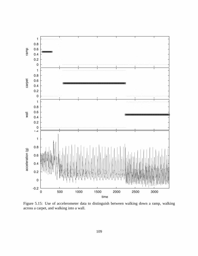
0 0.2 0.4 0.6 0.8

1

ram

p

0 0.2 0.4 0.6 0.8

1

carp

et

0 0.2 0.4 0.6 0.8

1

wal

l

-0.2

0

0.2

0.4

0.6

0.8

1

1.2

0 500 1000 1500 2000 2500 3000

acce

lera

tion

(g)

time

Figure 5.15: Use of accelerometer data to distinguish between walking down a ramp, walkingacross a carpet, and walking into a wall.

109

0 0.2 0.4 0.6 0.8

1w

all

0 0.2 0.4 0.6 0.8

1

play

ing

0 0.2 0.4 0.6 0.8

1

hook

ed

0 0.2 0.4 0.6 0.8

1

stan

ding

-2

-1.5

-1

-0.5

0

0 10000 20000 30000 40000 50000 60000

acce

lera

tion

(g)

time

Figure 5.16: Use of accelerometer data to distinguish between playing soccer, walking into a wall,walking with one leg caught on an obstacles, and standing still.

110

0 0.2 0.4 0.6 0.8

1br

ight

ligh

ts

0 0.2 0.4 0.6 0.8

1

med

ium

ligh

ts

0 0.2 0.4 0.6 0.8

1

dim

ligh

ts

0 0.2 0.4 0.6 0.8

1

light

s of

f

0

20

40

60

80

100

120

140

160

180

200

0 1000 2000 3000 4000 5000 6000 7000 8000

imag

e lu

min

ance

(0-2

55)

time

Figure 5.17: Use of average luminance from images to distinguish between bright, medium, dim,and off lights while playing soccer.

111

0 0.2 0.4 0.6 0.8

1br

ight

ligh

ts

0 0.2 0.4 0.6 0.8

1

med

ium

ligh

ts

0 0.2 0.4 0.6 0.8

1

dim

ligh

ts

0 0.2 0.4 0.6 0.8

1

light

s of

f

0

20

40

60

80

100

120

0 1000 2000 3000 4000 5000 6000 7000 8000 9000

imag

e lu

min

ance

(0-2

55)

time

Figure 5.18: Use of average luminance from images to distinguish between bright, medium, dim,and off lights while standing still.

112

Figure 5.17 shows the results from the first camera task distinguishing between bright, medium,dim, and off lights while the robot is playing soccer. This task is labelled as “lights playing” inthe results summary table. PSC was trained on one example sequence and tested on a completelyseparate sequence. Each class was trained using 1000 examples. PSC was tested on windows ofsize 50 (2 seconds of data), and was tested after every 25 data points. PSC performed fair overall,correctly classifying 64.69% of the test windows. Most of the errors were due to problems dis-tinguishing between bright lights and medium lights. Confusion errors between these two classesaccounted for 54% of the errors the algorithm made during this test.

Figure 5.18 shows the results from the second camera task distinguishing between bright, medium,dim, and off lights while the robot is standing still. The robot moved its head to look at differentobjects. This task is labelled as “lights standing” in the results summary table. PSC was trainedon one example sequence and tested on a completely separate sequence. Each class was trainedusing 150–200 examples. PSC was tested on windows of size 50 (2 seconds of data), and wastested after every 10 data points. As the graphs show, PSC excels at distinguishing between thesedifferent lighting conditions, achieving an accuracy of 93.77%.

5.7 Conclusion

We have presented an algorithm for generating predictions of future values of time series. We haveshown how to use that algorithm as the basis for a classification algorithm for time series. Weproved through testing that the resulting classification algorithm robustly detects a wide varietyof possible changes that signals can undergo including changes to mean, variance, observationnoise, period, and signal shape. The algorithm has the nice properties that the performance of thealgorithm improves when more training data is available, when more data is available before aclass label must be chosen, and when the difference between the signals becomes greater. Theseproperties should be expected of all prediction algorithms. The algorithm can be used to replace acollection of algorithms tuned to detecting particular changes in signals with one algorithm whichcan detect any change to the signal. We proved through testing on robotic sensor data that theresulting classification algorithm can be used to differentiate between semantically different signalclasses.

5.8 Summary

In this chapter, we developed version 1 of an on-line algorithm for environment identification/classificationof a time series. The algorithm is called the Probable Series Classifier. The algorithm makes fewassumptions and can detect a wide variety of types of changes in a time series. The algorithm onlyrequires an example signal from each environment to be identified and is thus easy to train. Thealgorithm has a strong probabilistic foundation. We proved the ability of the algorithm to detect

113

environment transitions both in simulated data and in data from real robots. In the next chapter, weimprove on this algorithm and further test the capabilities of the algorithm.

114

Chapter 6

Probable Series Classifier Version 2

In this chapter, we present and improved version of the Probable Series Classifier algorithm. Thisalgorithm builds upon and improves our initial version of the algorithm described in the previouschapter. This chapter can be read without reading the previous chapter, but an understanding ofthe previous chapter may help put some of the results in context. The algorithm provides general,robust, on-line environment identification given a relevant sensor signal to be used for recognitionand examples sensor signals from each of the environments to be recognized. The algorithm hasvery few parameters and the parameters it does have are easy to set. We analyze the performanceof the algorithm on a variety of simulated data and sensor signals from real robots and comparethe results with the previous version of the algorithm. We then apply the algorithm to a realisticrobotic task. We prove that using the algorithm for environment identification and adaptation leadsto improved performance of the robot.

6.1 Introduction

Noticing and adapting to changes is an important problem in many fields. We approach the prob-lem from the field of robotics where time series generated by sensors are readily available. We areinterested in using these signals to identify sudden changes in the robot’s environment allowing therobot to respond intelligently. For this application, the signal segmentation must be performed inreal time and on line, which requires algorithms that are amenable to on-line use. Usually a math-ematical model of the process that generates the sensor signal is unavailable. Therefore, we focuson techniques that require little a priori knowledge and few assumptions. Many researchers haveapproached this problem including Penny and Roberts [49] using autoregressive Hidden MarkovModels and Gharamani [20] using switching state-space models. This work differs from previ-ous work in being developed for practical robot application which requires properties not found inthese other techniques. A detailed description of these differences can be found in the related workchapter, Chapter 7.

115

In previous chapters (Chapter 4 and Chapter 5), we developed techniques for segmenting a timeseries into different classes given labelled example time series. In Chapter 5, we showed that ouralgorithm can successfully segment signals from robotic sensors. In this chapter, we improve onour previous technique by replacing a windowed approach to signal classification with a recursivesolution based on a simple Dynamic Bayes Net (DBN).

In this chapter, we apply our algorithm to a realistic robotic task. We adapt the technique fromthe previous chapter by showing how to successfully train the system in the presence of feedbackbetween the signal used for adaptation and the choices made by adaptation. We also show, for thefirst time, that using this adaptation results in a large improvement in the robot’s performance in anon-trivial task.

We have named our new algorithm for classifying time series the Probable Series Classifier (PSC).It is based on a time series prediction component which we will refer to as the Probable SeriesPredictor (PSP). Unlike many other methods, PSP predicts amulti-modelprobability density overnext values. PSC uses several PSP modules to classify a time series into one of a set number ofpre-trained states each of which corresponds to one environment. We will use the term state andenvironment interchangeably. PSC uses one PSP module per state/environment. Each PSP moduleis pre-trained from an example time series generated in one environment. PSP uses an internalnon-parametric model trained from an example time series to make its predictions. PSC runs eachPSP module on a time series to be classified and uses the one which best predicts the time seriesas the classification of the unknown time series. We take a very general approach where we detecta wide variety of types of changes to the signal which sets PSC apart from these other techniques.

PSC is a practical algorithm. PSC takesO(n log(n)) time forn observations in the current imple-mentation. The chief advantages of PSC over previous approaches are:

• PSC is capable of predicting a multi-modal distribution over values.

• PSC is amenable to on-line training as more data from a particular environment becomesavailable.

• PSC includes a dependence of each sensor reading on the previous sensor reading.

PSC requires no knowledge about the system structure, as it only requires labelled time seriesexamples. PSC also requires negligible training time since almost all of the work is done at querytime. While there are many methods from HMM research that predict a multi-modal distributionover values, we are not aware of any that condition on the previous time series value at the sametime.

6.2 System Model

In this section, we describe the class of systems for which we wish our algorithm to work. Thismodel is the same as in the previous chapter (Section 5.2). We describe the system model that

116

Figure 6.1: An example system with three states.

is assumed to generate the signals we process. Our algorithm is designed for detecting discreteenvironment changes of a system with a finite and known number of environments. We concen-trate primarily on the challenges created by real-world, noisy sensor streams and less on possiblecomplex relationships between states/environments.

A pictorial representation of a system with three states/environments is shown in Figure 6.1. Thetop part of the figure shows an example possible sensor signal from the robot’s sensors. Thisparticular example is from accelerometer data from an AIBO robot. This sensor signal is the inputto the algorithm. The underlying system is shown in the bottom half of the figure. The systemhas three states (S1,S2,S3). The robot may transition from any state/environment to any otherstate/environment as shown by the dark arrows. Each environment causes a characteristic patternof sensor signal readings. An example signal generated in each environment is shown as a mini-graph next to the state diagram. At any given time, exactly one environment is active and generatesthe sensor signal seen. In this case, the example signal shown in the top part of the graph is bestexplained as being generated from S1 until timestep≈ 450, S2 until timestep≈ 2200, and S3 forthe remaining time. The goal of the algorithm is to take the sensor signal at the top of the graphand produce the series of states/environments that generated it (as in the previous sentence) in anon-line fashion.

We will assume that the frequency of switching between different environments is relatively lowsuch that sequential sensor values are likely to be from the same environment. This assumption isvery reasonable for most robotic applications. Most sensors provide readings at rates of 25 times

117

Figure 6.2: A Dynamic Bayes Net model of signal generation.

per second or higher. We are usually interested in adapting to conditions that change slowly, lessthan one change per 5 seconds. Even at the slowest sensing rate and the fastest environmentalchange rate, we will have 125 sensor readings before the environment changes.

We take a maximum likelihood approach to the problem. At any given time, we would like toknow which state/environment is most likely to be the state/environment that is responsible for thecurrent sensor signal. More formally, we would like to find the state/environment indexi at timej, that maximizes

P (sj = i|~xj, ~xj−1, . . . , ~x0) (6.1)

where~xj is the observation vector at timej andsj is the current state at timej.

6.3 Probable Series Classifier Algorithm

In this version of the algorithm, we will replace our previous windowed approach with one based ona DBN. Our DBN model is shown in Figure 6.2. The states/environments the system goes throughover time are shown at the top half of the figure. The observations at various times are shown inthe bottom half of the figure. Each arrow in the figure corresponds to a conditional probabilitydependence. The dependencies which our algorithm keeps that a typical HMM approach ignoresare highlighted with thick, red arrows. The primary difference in our model is a dependence ofeach sensor reading on the previous sensor reading (in addition to the current environment). Thisextra dependence is important for robotics applications. In most cases, sensor readings that arenearby in time are highly correlated because the sensors update faster than the world changes.These sensor readings that are correlated are still within the same environment, however, becausethe environment changes we are interested in are ones that change at a slow enough rate to allowfor adaptation.

We will define the belief state at timej for state/environmenti as the probability of it being thecurrent environment at timej given all available information (Equation 6.1).

B(sj = i) = P (sj = i|~xj, ~xj−1, . . . , ~x0) (6.2)

118

We will like to simplify this equation into a form that we can use to calculate the most likely stateat any time. We proceed by simplifying the belief equation (Equation 6.2).

B(sj = i) = P (sj = i|~xj, ~xj−1, . . . , ~x0)

=P (~xj|~xj−1, . . . , ~x0, sj = i) · P (sj = i|~xj−1, . . . , ~x0)

P (~xj|~xj−1, . . . , ~x0)(6.3)

=P (~xj|~xj−1, . . . , ~x0, sj = i) · P (sj = i|~xj−1, . . . , ~x0)

β(6.4)

≈ νP (~xj|~xj−1, . . . , ~xj−m, sj = i) · P (sj = i|~xj−1, . . . , ~x0) (6.5)

In Equation 6.3, we have applied Bayes’ rule to Equation 6.2. In Equation 6.4, we note thatP (~xj|~xj−1, . . . , ~x0) is a normalizing constant that does not depend on the state. This normalizingconstant does not affect whichs = i has the maximum likelihood. We replace this expressionwith the constantβ which we invert in Equation 6.5 to produce the constantν. In Equation 6.5,we make themth-order Markov assumption that values> m time steps ago are negligible, givenmore current readings. This assumption/approximation simplifiesP (~xj|~xj−1, . . . , ~x0, sj = i) toP (~xj|~xj−1, . . . , ~xj−m, sj = i). This assumption is reasonable since sensor values from the distantpast are unlikely to be useful in predicting current sensor readings. We use a value ofm = 1in all of our tests. A value ofm = 0 reduces the update equations to those used in HMMs. Avalue ofm = 0 fails to condition on the previous sensor reading however. Our signals show astrong correlation between neighboring signal values and thus the assumption implied bym = 0is violated by our robotic data.

We now need to simplify the termP (sj = i|~xj−1, . . . , ~x0) in Equation 6.5.

P (sj = i|~xj−1, . . . , ~x0) =∑

l

P (sj = i, sj−1 = l|~xj−1, . . . , ~x0) (6.6)

=∑

l

P (sj = i|sj−1 = l, ~xj−1 . . . ~x0)P (sj−1 = l|~xj−1 . . . ~x0) (6.7)

=∑

l

P (sj = i|sj−1 = l, ~xj−1 . . . ~x0) ·B(sj−1 = l) (6.8)

=∑

l

P (sj = i|sj−1 = l) ·B(sj−1 = l) (6.9)

We begin by considering the joint distribution oversj = i andsj−1 = l and then marginalizingover sj−1 = l in Equation 6.6. In Equation 6.7, we use the fact thatP (A, B) = P (A|B)P (B)to rearrange the equation. We note thatP (sj−1 = l|~xj−1 . . . ~x0) = B(sj−1 = l) by definition(Equation 6.2) and use this substitution to produce Equation 6.8. We make the assumption that thecurrent state is conditionally independent of old observations (before timej) given the previousstate, i.e.P (sj = i|sj−1 = l, ~xj−1 . . . ~x0) = P (sj = i|sj−1 = l). This assumption is reasonablesince observations from the past are only useful for determining the previous state which we aregiven.

119

Returning to the belief equation (Equation 6.2), we can now create a recursive solution for updatingthe belief equation:

B(sj = i) = P (sj = i|~xj, ~xj−1, . . . , ~x0)

∝ P (~xj|~xj−1, . . . , ~x0, sj = i) · P (sj = i|~xj−1, . . . , ~x0) (6.10)

≈ νP (~xj|~xj−1, . . . , ~xj−m, sj = i) · P (sj = i|~xj−1, . . . , ~x0) (6.11)

= P (~xj|~xj−1 . . . ~xj−m, sj = i) ·∑

l

P (sj = i|sj−1 = l)B(sj−1 = l) (6.12)

Equations 6.10 and 6.11 come from Equations 6.4 and 6.5, respectively. Equation 6.12 is the resultof using Equation 6.9 to substitute forP (sj = i|~xj−1, . . . , ~x0).

We assume a uniform distribution over all possible initial states/environments. We also assumethatP (sj = i|sj−1 = l) = .999 if i = l and a uniform distribution of the remaining probabilityover other states. The transition probability does not effect the most likely state/environment atany given time much since the probability is dominated by the sensor readings. The self transitionprobability can be derived from the expected switching frequency and the data sampling rate. Forinstance, if the expected transition frequency is once every 30 seconds and the sensor readingsare available 25 times per second, we would expect one transition for every25 · 30 = 750 sensorreadings. So, we would expect to stay in the same state for749 out of 750 sensor readings for aprobability of 749/750 = .9986. The only term left to evaluate isP (~xj|~xj−1 . . . ~xj−m, sj = i).This term is evaluated by our Probable Series Predictor algorithm which is detailed in the nextsection. We usedm = 1 for all of our experiments.

This belief update equation is useful for segmentation and classification. Our Probable SeriesClassifier algorithm classifies a time series by finding the most likely state at the each time step,i.e. the state that maximizes the belief equation. Our algorithm runs in real time on a Athlon XP2700 processing data at 125Hz.

6.4 Probable Series Predictor Algorithm

In this section, we describe version 2 of our Probable Series Predictor Algorithm. This versionincludes several enhancements to the algorithm including: faster execution time, support for multi-dimensional data, and improved prediction accuracy. These improvements are achieved via a newmethod for output bandwidth selection, a bandwidth limited output kernel, and a new mixtureoutput model. These differences are highlighted in the description of the algorithm that follows.

We need a prediction of the likelihood of new time series values based upon previous values andthe current statei.

P (~xj|~xj−1, . . . , ~xj−m, sj = i)

Note, that statei is known in this case, so we know for which state we are generating a prediction.Assume we have previous time series values generated by this state. We can use these previous

120

base value

base value

outp

ut v

alue

outp

ut v

alue

wei

ght

probability

Figure 6.3: Data prediction. The dots in the main graph show the data available for use in predic-tion. The grey bar shows the range of values used in the prediction. The bottom graph shows theweight assigned to each model point. The left graph shows the contribution of each point to thepredicted probability of a value at time t as dotted curves. The final probability assigned to eachpossible value at time t is shown as a solid curve.

examples to generate an estimate at timej given the previous values of the time series. We willfocus on the case wherem = 1. Our examples in this section will focus on the case where~x is a single dimensional value. The segmentation results presented later in the chapter use asingle dimensional value for the simulation and robotic data segmentation tests. The robotic taskpresented later in the chapter uses the full three dimensions of the sensor signal.

We have: a set of value pairs~xi,~xi−1 and a value at timej−1 (~xj−1). We need to generate aprobability for each possible~xj. We can use non-parametric techniques with a locally weightedapproach. The problem is visualized in Figure 6.3. We need to introduce some terminology tomore easily discuss the problem.

base value(s)Those value(s) used in generating a predicted value. These are the time series valueson which the output is conditioned. In the case ofm = 1, this is just~xj−1. The conditioningon the state is accomplished by having a separate model for each state.

output value The value output by prediction.

121

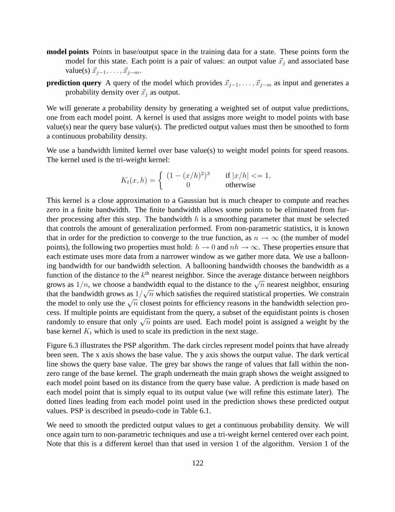
model points Points in base/output space in the training data for a state. These points form themodel for this state. Each point is a pair of values: an output value~xj and associated basevalue(s)~xj−1, . . . , ~xj−m.

prediction query A query of the model which provides~xj−1, . . . , ~xj−m as input and generates aprobability density over~xj as output.

We will generate a probability density by generating a weighted set of output value predictions,one from each model point. A kernel is used that assigns more weight to model points with basevalue(s) near the query base value(s). The predicted output values must then be smoothed to forma continuous probability density.

We use a bandwidth limited kernel over base value(s) to weight model points for speed reasons.The kernel used is the tri-weight kernel:

Kt(x, h) =

{(1− (x/h)2)3 if |x/h| <= 1,

0 otherwise

This kernel is a close approximation to a Gaussian but is much cheaper to compute and reacheszero in a finite bandwidth. The finite bandwidth allows some points to be eliminated from fur-ther processing after this step. The bandwidthh is a smoothing parameter that must be selectedthat controls the amount of generalization performed. From non-parametric statistics, it is knownthat in order for the prediction to converge to the true function, asn → ∞ (the number of modelpoints), the following two properties must hold:h→ 0 andnh→∞. These properties ensure thateach estimate uses more data from a narrower window as we gather more data. We use a balloon-ing bandwidth for our bandwidth selection. A ballooning bandwidth chooses the bandwidth as afunction of the distance to thekth nearest neighbor. Since the average distance between neighborsgrows as1/n, we choose a bandwidth equal to the distance to the

√n nearest neighbor, ensuring

that the bandwidth grows as1/√

n which satisfies the required statistical properties. We constrainthe model to only use the

√n closest points for efficiency reasons in the bandwidth selection pro-

cess. If multiple points are equidistant from the query, a subset of the equidistant points is chosenrandomly to ensure that only

√n points are used. Each model point is assigned a weight by the

base kernelKt which is used to scale its prediction in the next stage.

Figure 6.3 illustrates the PSP algorithm. The dark circles represent model points that have alreadybeen seen. The x axis shows the base value. The y axis shows the output value. The dark verticalline shows the query base value. The grey bar shows the range of values that fall within the non-zero range of the base kernel. The graph underneath the main graph shows the weight assigned toeach model point based on its distance from the query base value. A prediction is made based oneach model point that is simply equal to its output value (we will refine this estimate later). Thedotted lines leading from each model point used in the prediction shows these predicted outputvalues. PSP is described in pseudo-code in Table 6.1.

We need to smooth the predicted output values to get a continuous probability density. We willonce again turn to non-parametric techniques and use a tri-weight kernel centered over each point.Note that this is a different kernel than that used in version 1 of the algorithm. Version 1 of the

122

Table 6.1: Probable Series Predictor algorithm.

ProcedurePredictOutput(generatormodel,basevalues)let OP ← generatormodel.modelpointslet D ← dist(OP.basevalues,basevalues)Choosebasedistequal to thed

√neth smallestd ∈ D.

let hb ← basedist+ noisebaselet pred ← {z.output value| z ∈ OP∧

dist(z.basevalues, basevalues) < hb}Perform correlation correction onpred.let base← {z.basevalues| z ∈ OP∧

dist(z.basevalues, basevalues) < hb}Choosehi,o ∝ distance(d

√neth) nearest prediction.

Return probability density equal topdf(z) =

∑i Kg(predi − z, hi,o)∗

Kt(basei − basevalues, hb)

algorithm used a Gaussian kernel. Because this kernel has a finite bandwidth, it may assign a zeroprobability to some points. This assignment is undesirable since we never have enough trainingdata to be absolutely sure the data could not have occurred in this state/environment. A similarproblem occurred with the Gaussian kernel, but in that case instead of the probability reaching zero,it merely became extremely close to zero. To overcome this problem, we assume the sensor valuesare generated according to a mixture model where the sensor value is generated with probability.9999 from the probability density defined by the sum of tri-weight kernels and with probability.0001 from a uniform distribution. Hence, we assign a .0001 probability that the time series valueis generated from a uniform distribution and a .9999 probability that it is generated according tothe estimated distribution. This assumption can be considered as a kind of prior belief about thedistribution of sensor values.

We need a method for selecting a bandwidth forKg, the output kernel. We use a modified form ofthe ballooning method. For each output value prediction, we assign a bandwidth proportional to thedistance to the

√n

th nearest output value with a minimum bandwidth. We used a proportionalityconstant of 0.5. In the previous version of the algorithm, we used a bandwidth that was the samefor every output value example point and used cross validation to select an appropriate bandwidth.We found that the proportional bandwidth selection method produced similar performance but ranabout 10 times faster than the previous method. We also found that this new bandwidth selectionmethod resulted in better modeling of the probability distribution in the tails were less data isavailable. With all points having the same bandwidth, outlying data points in the tails of thedistribution were forced to have a small bandwidth because of points in the most likely parts of thedistribution. These small bandwidths on outlying points resulted in a lumpy representation whichpoorly represented the actual uncertainty in the parts of the probability distribution for which less

123

example data is available. By choosing bandwidths separately for each point, points in the tailsof the distribution can have larger bandwidths without affecting the rest of the distribution. Wefound that the algorithm is very insensitive to the exact proportionality constant used. We didn’tnotice any change in performance for proportionality constants from .1 to 1.0. This new bandwidthselection scheme allowed us to easily scale the algorithm up to more dimensions.

As exemplified in Figure 6.3, there is usually a strong correlation between the time series valueat timet and the value at timet − 1. This correlation causes a natural bias in predictions. Modelpoints with base values below the query base value tend to predict an output value which is toolow and model points with base values above the query base value tend to predict an output valuewhich is too high. We can correct for this bias by compensating for the correlation betweenxt andxt−1. We calculate a standard least squares linear fit betweenxt−1 andxt. Using the slope of thislinear fit, we can remove the bias in the predicted output values by shifting each prediction in bothbase value and output value until the base value matches the query base value. This process canshift the predicted output value a substantial amount, particularly when using points far from thequery base value. This process improves the accuracy of the algorithm slightly. This correlationremoval was used in all the tests performed in this thesis.

124

6.5 Evaluation in Simulation

We tested PSC using simulated data, allowing us to know the correct classification ahead of time.It also allowed us to systematically vary different parameters of the signal to see the response of theclassification algorithm. We used a similar testing methodology as for version 1 of the algorithm.The testing methodology was modified to take into account the new window-less nature of thealgorithm.

We used PSC to segment a signal generated from a 2 state generator. One state was a fixed baselinesignal. The other state was a variation of the baseline signal formed by varying one parameter ofthe signal. The algorithm was graded on its ability to correctly label segments of the signal that ithadn’t been trained on into the 2 states. We tested the performance of PSC by varying the followingtest parameters:

Training window size The number of data points used to train on each state. The smaller thewindow size the harder the problem.

Parameter value The value of the parameter used in the modified signal. The closer the parameterto the baseline value the harder the problem.

Parameter modified The parameter chosen for modification. We tested changes to the followingparameters: mean, amplitude/variance, observation noise, and period.

For each test we generated a time series with 4000 data points. The baseline state (class 1) gen-erated the first and third quarter of the data signal and the modified state (class 2) generated thesecond and fourth quarter of the data. We chose to use a sine wave for the underlying signal forthe baseline. We added uniform observation noise to this underlying signal to better reflect a realworld situation. The signal is parameterized by amplitude, mean, period, and noise amplitude re-sulting in 4 parameters. The standard signal used an amplitude of5 ∗ 105, a mean of0, a periodof 20 observations, and a noise amplitude of5 ∗ 104, resulting in±10% noise on each observationrelative to the signal range.

For each test, we trained a model of each state on an example signal from that state. This examplesignal was not included in the testing data. The length of the example signal (training window) wasvaried from 5 data points to 100 data points to show the effect on the results. We tested with 14different example signals for each state and averaged the results. For each test, we calculated thefraction of time the most likely state matched the actual state of the system. Note that in testing thisversion of the algorithm, we determine a most likely state at each time point whereas with version1 of the algorithm we only determined a mostly state at the end of select windows of data. Thisfraction is reported on all of the result figures. A value of1 indicates a perfect segmentation of thetest segments into classes. A value of0.5 is the performance expected from randomly guessing theclass. This metric equals the probability of getting the correct labelling using a random trainingexample signal for each class.

We summarized our test results in a series of figures. The y axis shows the fraction of correctlabellings achieved by PSC. In each figure, there is a point at which the performance of PSC falls

125

to chance levels (0.5). These points occur where the states for class 1 and class 2 have the sameparameters and are hence generate the same signal. Since a signal cannot be segmented from itself,we expect the algorithm’s performance to fall to chance levels at these points. We gathered resultspertinent to applications where a constant amount of training data is available as would occur inon-line labelling applications.

Figure 6.4 shows the performance of PSC with respect to changes in the amplitude of the signal.PSC performs quite well even for small training window sizes. This type of change to the signalwould not be detected by algorithms that are only sensitive to mean shifts as a change in amplitudedoes not change the mean but only the variance.

Figure 6.5 shows the performance of PSC with respect to mean shifts. PSC performs well and isable to detect small mean shifts. This type of change to the signal can be detected by algorithmscapable of detecting mean shifts. Many mean shift algorithms would have trouble with a periodicsignal like this sine wave, though, unless the data was averaged over a full period which wouldslow detection time.

Figure 6.6 shows the performance of PSC with respect to changes in observation noise. This typeof change is very difficult to detect as it produces no mean shift in the signal and a negligiblevariance change. Nevertheless, PSC is still able to detect this type of change effectively. Manyalgorithms fail to detect this kind of change to a signal.

Figure 6.7 shows the performance of PSC in detecting changes in the period of the signal. PSCperforms well at detecting a change of the period most of the time. PSC fails to detect the changein the period for the case where the period is longer than the training sequence but in this case thetraining signal is not fully representative of the full signal for the state.

126

0.4

0.5

0.6

0.7

0.8

0.9

1

200000 400000 600000 800000 1e+06 1.2e+06 1.4e+06 1.6e+06 1.8e+06 2e+06

frac

tion

corr

ect

amplitude

win size 20win size 40win size 80win size 100

Figure 6.4: Detection of changes to the signal amplitude with a fixed training window size. The xaxis shows the factor by which the amplitude was multiplied.

0.4

0.5

0.6

0.7

0.8

0.9

1

0 0.5 1 1.5 2

frac

tion

corr

ect

mean shift

win size 20win size 40win size 80win size 100

Figure 6.5: Detection of changes to the signal mean with a fixed training window size. The x axisshows the mean shift as a fraction of the signal amplitude.

127

0.4

0.5

0.6

0.7

0.8

0.9

1

0.05 0.1 0.15 0.2 0.25 0.3 0.35 0.4

frac

tion

corr

ect

noise amplitude

win size 20win size 40win size 80win size 100

Figure 6.6: Detection of changes to the observation noise with a fixed training window size. The xaxis shows the observation noise as a fraction of the signal amplitude.

0.4

0.5

0.6

0.7

0.8

0.9

1

10 20 30 40 50 60 70 80

frac

tion

corr

ect

period

win size 20win size 40win size 80win size 100

Figure 6.7: Detection of changes to the period with a fixed training window size. The x axis showsthe period of the signal.

128

6.6 Evaluation on Robotic Data

We evaluated the Probable Series Classifier (PSC) using data logged by our robot as it performedvarious tasks. The data was hand classified as a baseline for comparison with the automatic classi-fication. We used a standard Sony AIBO ERS-210 for gathering all of our data.

6.6.1 Methodology

We generated a set of data series from the sensors on our robot. We used two different sensors, aCMOS camera and an accelerometer. Since our PSC implementation currently only supports singledimensional data, we reduced each data series down to a single dimensional data series. Eachcamera image was reduced to an average luminance value (a measure of brightness), resulting in a25Hz luminance signal. The accelerometer data is inherently three dimensional with accelerationsalong three axes. We chose to use the axis oriented towards the front of the robot (the other axesgave similar results). The accelerometer data has a frequency of 125Hz. For each task, PSC wastrained on a segment of data for each possible class. PSC used a window of data to generateeach classification starting at the data item to be classified and extending backwards in time, i.e.only data that would be available in an on-line scenario was used for classification. The PSCgenerated label was compared to a hand generated label to ascertain accuracy. In some of thesignals, there were segments of the test signal that did not correspond to any of the trained classes.These segments were not used in calculating accuracy. We considered a total of five differentclassification tasks.

6.6.2 Results

Each figure show the results from one task. The bottom part of each figure shows the raw datasignal used for testing. Each of the other figures corresponds to one of the trained classes. Theclass to which it corresponds is labelled to the left of each graph. The thick black line runningthrough parts of each class graph indicates when this class is the correct class according to thehuman generated labelling. The small black dots show the probability that PSC assigned to thisclass at each point in time (based on a window of data prior to this time point). Ideally, theprobability would be 1.0 when the thick black bar is present and 0.0 otherwise. In sections wherethe test data series does not correspond to any of the trained classes, the indicator bar is absent andthe output of PSC for each class is irrelevant. Table 6.2 summarizes the results achieved by PSC.The column labeled “PSC v.1” shows the performance of our previous window based approach(Chapter 5). The column labelled “PSC v.2” shows the accuracy of our new DBN based approach.As the table shows, we see a significant reduction in errors by employing the DBN model.

We also compared the results generated by using an HMM model. The HMM model was con-structed by removing the dependency on the previous sensor reading in the PSC v.2 algorithm.This dependence was removed by artificially placing all model points’ base values at the query’s

129

Table 6.2: Accuracy of PSC in various test classification tasks.

Task Sensor PSC v.1 PSC v.2 HMMWalk stability Accelerometer 99.19% 98.26% 63.77%Walk floors Accelerometer N/A 93.22% 56.12%

Walk interference Accelerometer 78.49% 85.62% 62.84%Lights playing Camera 64.69% 82.01% 57.17%Lights standing Camera 93.77% 99.98% 99.90%

base value, i.e. acting as if all model points are perfectly relevant for all queries. This methodologyresults in an HMM model that has an output density defined by a non-parametric density. Theoutput density is a sub-sampled version from all the model points due to the limitation imposedon the number of points used in forming the density. This limitation to using

√n data points is in

place for efficiency reasons and is consistent between the PSC v.2 and HMM tests.

Figure 6.8 shows the results from the first accelerometer task distinguishing between walking downa metal ramp, across a soft carpet, and into a low wooden wall. This task is labelled as “walk sta-bility” in the results summary table. PSC was trained on one example sequence and tested ona completely separate sequence. Each class was trained using 500 examples, except 400 exam-ples were used for training the “ramp” class. As the graphs show, PSC does an excellent job ofdistinguishing between these different walking conditions achieving and accuracy of 98.26%.

Figure 6.9 shows the results from the second accelerometer task distinguishing between walkingin place on cement, hard carpet, and soft carpet. This task is labelled as “walk floors” in the resultssummary table. PSC was trained on one example sequence and tested on a completely separatesequence. As the graphs show, PSC does an excellent job of distinguishing between these differentwalking conditions achieving and accuracy of 93.22% despite the similarity between the two typesof carpet.

Figure 6.10 shows the results from the third accelerometer task distinguishing between playingsoccer, walking into a wall, walking with one leg hooked on an obstacle, and standing still. Theplaying class includes a wide variety of signals including walks in several different directionsand full body kicking motions such as diving on the ball. Small portions of the playing class,include standing in place making these sections look like the standing operating environment. Thistask is labelled as “walk interference” in the results summary table. PSC was trained on examplesequences from the test sequence. In other tests, we did not observe a noticeable difference betweentesting on training data and testing on separate testing data. Each class was trained using 5000examples. PSC performed well overall, correctly classifying 85.62% of the data points. PSCperformed perfectly on the standing still data. It had the most problems identifying hooked on anobstacle, often confusing it with playing.

Figure 6.11 shows the results from the first camera task distinguishing between bright, medium,dim, and off lights while the robot is playing soccer. This task is labelled as “lights playing” in

130

the results summary table. PSC was trained on one example sequence and tested on a completelyseparate sequence. Each class was trained using 1000 examples. PSC performed fairly well over-all, correctly classifying 82.01% of the data points. Most of the errors were due to problemsdistinguishing between bright lights and medium lights.

Figure 6.12 shows the results from the second camera task distinguishing between bright, medium,dim, and off lights while the robot is standing still. The robot moved its head to look at differentobjects. This task is labelled as “lights standing” in the results summary table. PSC was trainedon one example sequence and tested on a completely separate sequence. Each class was trainedusing 150–200 examples. Although this is an easy classification task, it is important to test thatthe algorithm works on both easy and difficult tasks to ensure practicality of the algorithm. PSCpasses easily achieving 99.98% accuracy.

131

0

0.2

0.4

0.6

0.8

1

ram

p

0

0.2

0.4

0.6

0.8

1

ca

rpe

t

0

0.2

0.4

0.6

0.8

1

wa

ll

-0.2

0

0.2

0.4

0.6

0.8

1

1.2

0 500 1000 1500 2000 2500 3000

acce

lera

tio

n (

g)

time

Figure 6.8: Use of accelerometer data to distinguish between walking down a ramp, walking acrossa carpet, and walking into a wall.

132

0

0.2

0.4

0.6

0.8

1

cem

ent

0

0.2

0.4

0.6

0.8

1

soft c

arp

et

0

0.2

0.4

0.6

0.8

1

hard

carp

et

-0.1

0

0.1

0.2

0.3

0.4

0.5

0.6

0.7

0.8

0 20000 40000 60000 80000 100000

accele

ration (

g)

time

Figure 6.9: Use of accelerometer data to distinguish between walking in place on cement, hardcarpet, and soft carpet.

133

0

0.2

0.4

0.6

0.8

1

wall

0

0.2

0.4

0.6

0.8

1

pla

ying

0

0.2

0.4

0.6

0.8

1

hooked

0

0.2

0.4

0.6

0.8

1

standin

g

-2

-1.5

-1

-0.5

0

0 10000 20000 30000 40000 50000 60000

acce

lera

tion

(g)

time

Figure 6.10: Use of accelerometer data to distinguish between playing soccer, walking into a wall,walking with one leg caught on an obstacles, and standing still.

134

0

0.2

0.4

0.6

0.8

1

bright lig

hts

0

0.2

0.4

0.6

0.8

1

mediu

m li

ghts

0

0.2

0.4

0.6

0.8

1

dim

lights

0

0.2

0.4

0.6

0.8

1

lights

off

0

20

40

60

80

100

120

140

160

180

200

0 1000 2000 3000 4000 5000 6000 7000 8000

imag

e lu

min

ance

(0-2

55)

time

Figure 6.11: Use of average luminance from images to distinguish between bright, medium, dim,and off lights while playing soccer.

135

0

0.2

0.4

0.6

0.8

1

bright lig

hts

0

0.2

0.4

0.6

0.8

1

mediu

m lig

hts

0

0.2

0.4

0.6

0.8

1

dim

lig

hts

0

0.2

0.4

0.6

0.8

1

lights

off

0

20

40

60

80

100

120

0 1000 2000 3000 4000 5000 6000 7000 8000 9000

imag

e lu

min

ance

(0-2

55)

time

Figure 6.12: Use of average luminance from images to distinguish between bright, medium, dim,and off lights while standing still.

136

Table 6.3: Training method for Probable Series Classifier.

ProcedureGenerateTrainingSignals()defineT j

i = training signal for class i on iteration jdefineT j

? = {T j1 , T j

2 , . . . , T jn}

for i = 1 to nT 0

i = signal recorded from robot while in environmenti while adaptation cycles through statesfor j = 1 to z

Train PSC usingT j−1? .

for i = 1 to n

T ji = signal recorded from robot while in environmenti while using PSC for adaptation

return T z?

6.7 Training in the Presence of Feedback

We would like to use the Probable Series Classifier (PSC) to perform a simple ball chasing taskacross 3 different environments. Each environment has different lighting conditions and requiresdifferent vision thresholds. For a discussion of our vision system, see Section 2.5. We would likePSC to identify the current area in which the robot is operating (lab/hallway/office) and choosethe matching thresholds. In order to use the algorithm, we must provide an example time seriesfor each environment. The example time series should match the time series the robot sees whenperforming the task while doing adaptation as much as possible. A complication arises, though,because the selection of thresholds to use affects the output of vision, which affects the behaviorof the robot, which affects the images captured by the robot’s camera, which affects the feedbacksignal used for adaptation. Thus, the fact that adaptation is occurring and affecting the signal usedfor adaptation creates an interesting feedback loop.

Figure 6.13 shows the movement of information in the complete system. The first feedback loopgoes from behaviors to world to camera to vision and back to behaviors. This loop corresponds tothe task of chasing the ball. This loop responds to the relative position of the ball to the robot inorder to ensure that the robot successfully tracks the ball and reaches it. We are trying to optimizethe performance of this loop and thus the adaptation feeds into one component of this loop to tryto improve its performance, namely, vision. The second feedback loop goes from behaviors toworld to camera to adaptation to vision and back to behaviors. This feedback loop complicatesthings because the signal that we are trying to use to optimize the first feedback loop changes aswe perform the adaptation.

We need a training signal that reflects the feedback signal we should expect for each environment.This feedback signal depends on the choices of the adaptation, however, and hence on the trainingsignal we provide the adaptation. We solve this circular dependency using an iterative technique

137

Figure 6.13: Information flow and feedback loops for the ball chasing task.

similar to Expectation Maximization. The idea is to provide successive approximations to the feed-back signal to expect in the final system with each feedback signal being a better approximationthan the last. We start with a poor approximation of the expected feedback signal and improveit each iteration. Each iteration using the signals from the previous iteration as a better exampleof the expected feedback signal. The entire process is shown in pseudo-code form in Table 6.3.Note, that although the method is presented in pseudo-code form, the procedure involves humaninteraction to place the robot in the appropriate environment to gather each training signal. Wegathered 30 seconds of data for each example signal for each iteration, except for the last iterationwe gathered 120 seconds of data to provide a larger number of examples. We did 4 iterations (z =4) and noticed an improvement on each iteration with diminishing returns on each iteration. Thefinal example signals gathered were used in all the tests that follow.

6.8 Evaluation in a Robotic Task

We evaluated the Probable Series Classifier (PSC) and our training method by running a number oftrials of a ball chasing task. The task consists of chasing an orange colored ball through three dif-ferent areas: a lab, a hallway, and an office. The environments are unstructured and contain manyobjects that are various shades of red, orange, and brown. The lighting conditions between theenvironments are different and change the apparent color of orange as seen by the camera. When

138

the robot reaches the ball, it is moved to the next in a list of static waypoints by a human. We testedusing PSC to identify the current area and choose appropriate threshold against 4 different staticthresholds, one trained on each environment (3 thresholds) and one trained on all environments atonce (1 threshold).

6.8.1 Methodology

We defined a ball chasing task for chasing an orange ball through 3 different areas (a lab, a hallway,and an office) each with a different lighting conditions. The robot was started in the lab at a setposition marked with clear tape. A number of waypoints were marked on the floor with clear tape.Each waypoint was 1 meter away from the previous waypoint. This distance is non-trivial for therobot to see the ball, but well within the maximum vision range of approximately 3 meters in idealconditions. The robot was started by pressing a button and was programmed to run towards theball while keeping the camera looking at the ball. If sight of the ball was lost, the robot wouldspin in place and scan with the head until the ball was seen again. Whenever the robot touched theball, the ball was immediately moved to the next waypoint by a human experimenter. The robotwas given 30 seconds to reach the next ball waypoint position after successful reaching the ball. Atotal of 9 waypoints were defined, which resulted in a total travel distance of the robot of 9 meters.The robot itself is about 20cm long. The waypoints were set up such that the robot travels 3 metersin each area on a fully successful journey. If the robot reached the end, the trial was stopped anddeemed a success. The furthest waypoint reached by the robot on each run was recorded.

The setup is shown in Figure 6.14. The starting location is marked with a black x and is justoff the right side of the image. Each waypoint is marked in the image with a black dot and anumeric identifier. The actual waypoints were marked with clear tape so as not to interfere withvision. Waypoint 3 is on the boundary between lab and hallway and waypoint 6 is on the boundarybetween hallway and office. The lab environment was much brighter than the either the hallway ofthe office. The hallway and the office had somewhat different color temperatures which affectedthe appearance of the ball.

Vision used a simple lookup table (thresholds) mapping pixel color in YCrCb color space to ball,floor, or background. Connected components was run on the resulting image and the resultingconnected region were analyzed to look for a ball. The ball was defined by the vision system asany vaguely round, orange object of approximately the right size and height off the ground, againsta background of floor. The thresholds were generated using a supervised learning algorithm. Ex-ample images were taken in each environment and hand labeled as ball, floor, or background. Theresulting labeled example set of pixels is used to generate the threshold table trying to maximizegeneralization without sacrificing accuracy on the training set. The vision system and thresholdlearning tools were developed as part of the CMPack RoboCup legged team [61].

We tested 5 different conditions. We tested using PSC to select the appropriate threshold to use ateach frame. We also tested using static thresholds trained on all 3 areas. Finally, we tested usingstatic thresholds trained on just one of the areas for each possible area.

139

Figure 6.14: Setup for the ball chasing task. Each waypoint is marked in the image with a black dotand a numeric identifier. The actual waypoints were marked with clear tape so as not to interferewith the vision of the robot. The robot and ball are visible in the picture between waypoints 3 and4.

140

Table 6.4: Success in a ball chasing task versus thresholds.

Forward Direction Reverse DirectionThresholds Successes Success RateSuccesses Success RateAdaptation (PSC) 5/10 50% 10/10 100%Static (All) 0/10 0% 0/10 0%Static (Lab) 0/10 0% 0/10 0%Static (Hallway) 1/10 10% 9/10 90%Static (Office) 0/10 0% 0/10 0%

After testing the robot’s performance in this task, we reversed the direction of travel to have therobot start in the office and travel to the lab. By having the robot travel in both directions, wecan verify the ability of the algorithm to detect all physically possible transitions between environ-ments. The forward direction tests lab to hallway and hallway to office transitions while the reversedirection tests hallway to lab and office to hallway transitions. We were unable to test office to laband lab to office transitions because the office and lab are not physically contiguous. Interestingly,the different directions were very different in terms of difficulty and the adaptation process wasrobust in providing a benefit in both the difficult and easy directions. The same waypoints wereused for this test, with the robot starting at waypoint 9 and proceeding to the x (waypoint 0). Wetested under the same 5 conditions as the other direction of travel.

Finally, we tested the ability of the robot to reach waypoints in each environment with each possiblethreshold. For each environment and threshold combination, we tested the ability of the robot toreach the ball at one waypoint from a nearby waypoint. We tested each waypoint traversal anddirection an equal number of times using the same rules as for the full task (30 seconds to reachthe ball). We started the robot looking at the ground to simulate the loss of tracking of the ballthat occurs when the ball is moved in the full task. We performed a total of 60 trials for eachenvironment/threshold combination. These tests allow us to make a theoretical model to predictthe robot’s performance to provide a baseline to compare our adaptation results against.

6.8.2 Results

The results of the experiment are shown in Figures 6.15 and 6.16 for the forward and reversedirections, respectively. The x axis of this graph shows the waypoint number. The y axis showsthe number of times this waypoint was successfully reached out of 10 runs. The lines on the graphhave been artificially separated slightly to improve visibility. The number of successful runs isan integer number in all cases. Since trials were stopped as soon as the robot failed to reach awaypoint in 30 seconds, the number of successes is monotonically non-increasing for successivelyhigher waypoint numbers (or successively lower in the case of the reverse direction).

The main thing to notice from this graph is the number of successes for which the robot made

141

0 1 2 3 4 5 6 7 8 90

1

2

3

4

5

6

7

8

9

10

Waypoint Number

Num

ber

of S

ucce

ssfu

l Tria

lsAdaptationStatic (All)Static (Lab)Static (Hallway)Static (Office)Theoretical Adapt.

Figure 6.15: Results from the ball chasing task in the forward direction. The x axis shows thewaypoint number. The y axis counts the successes in reaching this waypoint out of 10 runs.

01234567890

1

2

3

4

5

6

7

8

9

10

Waypoint Number

Num

ber

of S

ucce

ssfu

l Tria

ls

AdaptationStatic (All)Static (Lab)Static (Hallway)Static (Office)Theoretical Adapt.

Figure 6.16: Results from the ball chasing task in the reverse direction. The x axis shows thewaypoint number. The y axis counts the successes in reaching this waypoint out of 10 runs.

142

it to the last waypoint. The robot successfully made it to the last waypoint on 5 out of 10 trialswhile using PSC for adaptation and only 1 out of 10 trials for the best set of static thresholds in theforward direction. This result is summarized in Table 6.4. Using adaptation resulted in a five-foldincrease in number of successful runs. In the reverse direction, adaptation had a perfect successrate but a static threshold also did very well successfully completing 9 out of 10 trials.

The reason for the large difference in successes is mostly due to the movement between waypoint1 and 2. Going from waypoint 1 to 2, there are distracting objects that can be mistaken for balldirectly in front of the robot while the real ball is somewhat to the side of the robot. When goingfrom waypoint 2 to 1, the distracting objects are well to the side of robot and sometimes partiallyoccluded while the ball is still slightly to the side of the robot. The behaviors are biased towardsnoticing objects in front of the robot since these locations can be seen during the kicking motionperformed when the robot reaches the ball. So, for the forward direction, this is a difficult transitionbecause of the confusing objects directly in front of the robot. For the reverse direction of travel,this transition is much easier, because the distracting objects are so far to the side of the robot.

During testing, we observed that the thresholds trained for the office saw the carpeting in the lab asthe ball. This problem can be seen analytically with the poor performance of the office thresholdsin the lab environment as shown in Table 6.5. These thresholds still had some successes becausethe grey mat is not mistaken for the ball. We also observed that avoiding seeing spurious balls inthe lab resulted in being unable to see the ball in the office. We also noticed some interferencebetween the color of the ball in the hallway and the lab carpeting but this was far less severe. Thethresholds trained for the hallway seemed to be a compromise, unlikely to see spurious balls in thelab, somewhat reduced ball vision in the hallway, and poor vision of the ball in the office.

Looking at the results more closely, we see that using the thresholds trained on the lab performedvery well for the 3 waypoints located in the lab and was unable to successfully traverse the hallway.The thresholds trained on the hallway performed well for the first 2 waypoints and often failed onwaypoint 3 which is on the border between the lab and hallway. These failures can mostly beattributed to the robot confusing an orange colored toolbox for the ball and wandering off into thelab. The lab thresholds did not suffer this problem because they successfully labeled the toolbox asbackground. The hallway thresholds performed reasonably well once the robot was in the hallwayand office. The progress in the office was slow but steady with the robot often losing the ball andre-acquiring it. The office thresholds never progressed far due to mistaking the carpeting in the labfor the ball most of the time.

Using thresholds trained on all 3 areas resulted in slightly worse performance in the lab comparedto the lab thresholds due to a higher confusion rate of seeing other objects as the ball. Thesecombined thresholds worked well in the hallway also, but completely failed to be able to see theball in the office. This failure is caused by the identical pixel colors being observed on the ball inthe office and the carpeting in the lab. Using adaptation (PSC) to choose the thresholds, we seethe thresholds perform slightly worse in the lab than the lab thresholds or thresholds trained on allareas. Using adaptation, the robot had some difficulty making the transition to the hallway as seenby the 2 failures to get from waypoint 3 to waypoint 4. At this point, the robot is standing on theborder between the lab and hallway. If the robot loses the ball at this point and spins to search

143

Table 6.5: Success rates for reaching waypoints per environment and threshold.

ThresholdEnvironment Lab Hallway Office

Lab 60/60 ( 100.00% ) 43/60 ( 71.67% ) 23/60 ( 38.33% )Hallway 22/60 ( 36.67% ) 54/60 ( 90.00% ) 45/60 ( 75.00% )Office 0/60 ( 0.00% ) 48/60 ( 80.00% ) 58/60 ( 96.67% )

Table 6.6: Adaptation perfomance compared to best possible threshold.

Environment Successes Best Threshold % of BestLab 55/57 ( 96.49% ) 100.00% 96.49%

Hallway 47/50 ( 94.00% ) 90.00% 104.44%Office 45/45 ( 100.00% ) 96.67% 103.44%

for it, the camera is switching taking images from the hallway and lab at a high rate. This rapidswitching increases the chance of the wrong thresholds being chosen and the robot being confusedby another object. We also see, however, that with adaptation, the robot has no trouble seeing theball in the office as the conflict between the ball color in the office and the carpet color in the labis avoided. Adaptation is the only method that successfully sees the ball most of the time in all 3areas.

We can attempt to model the theoretical best results for adaptation by attempting to model theprobability of success at several sub-tasks, namely, the task of moving from one waypoint to thenext. The probability of successfully completing the full task of chasing the ball from the startingwaypoint to the final waypoint can be approximated by the probability of reaching each waypointfrom the previous waypoint given the thresholds that are being used. For example, the probabilityof reaching waypoint 9 from waypoint 0 using the hallway thresholds the entire way can be ap-proximated byp3

lhp3hhp

3oh wherepoh is the probability of successfully traversing one waypoint in

the office environment using hallway thresholds. Reading from Table 6.5, we see thatplh = .7167,phh = .9, andpoh = .8. Using this model, we would predict that using hallway thresholds, wewould successfully reach waypoint 9p3

lhp3hhp

3oh = .137 or 13.7% of the time. This prediction is a

fairly close match for the results of the forward prediction, but a horrible prediction for the reversedirection. The problem is that the probability of successfully traversing from one waypoint to thenext depends on the particular waypoints involved and the direction of travel. As discussed in theprevious paragraph, the traversal from waypoint 1 to 2 is much harder than the other waypointtraversals in the lab environment.

A similar model can be constructed for a theoretical perfect adaptation using the available thresh-olds. A perfect adaptation would always use the thresholds for the current environment. Fortraversing from waypoint 0 to waypoint 9, we would expect a success rate ofp3

llp3hhp

3oo = .6586

144

or 65.9%. This expectation is higher than the actual success rate of50% achieved in the forwarddirection but lower than the100% success rate achieved in the reverse direction. The expectednumber of successes based on this model are shown in Figures 6.15 and 6.16 as the dashed linelabeled “Theoretical Adapt.”. Overall performance is on par with that expected from a theoreticalbest case adaptation, but is impossible to give a quantitative measure of performance without amore accurate model.

Finally, we compare the performance of the adaptation method to the best static threshold at reach-ing single waypoints in each environment. These results are summarized in Table 6.6. Lookingclosely at the graphs of the adaptation performance for the forward and reverse directions, we seethat there are a total of 57 times that the robot needed to travel from one waypoint to the nextwaypoint in the lab environment. Out of these 57 waypoint traversals, 55 were successful. Re-sults for the hallway and office environments can be summarized in the same manner. The beststatic threshold for each environment is the one that matches the environment. The performanceof these static thresholds in the correct can be seen in Table 6.5 along the diagonal. These resultsare repeated in the column “Best Threshold” in Table 6.6. We would expect a perfect adaptationto always select the thresholds which match the current environment. By always selecting thethresholds matching the current environment, the adaptation should match the performance of thestatic thresholds. Any deviation from the thresholds for the current environment would be expectedto hurt the performance of the robot. Accordingly, we compare the success rate with adaptationto the best static thresholds. Surprisingly, the adaptation actually performs better than the staticthreshold even for the environment for with the static threshold was specifically developed. Theperformance of adaptation compared to the best static threshold is listed in column “% of Best”in Table 6.6. The results show that adaptation performs nearly as well as static thresholds in thelab environment and slightly better than static thresholds in the hallway and office environments.In retrospect, this outcome shouldn’t be so surprising. Each environment encompasses differentconditions within the same room. The adaptation can exploit these differences for better perfor-mance by using thresholds for other environments for the more unusual parts of each environment.It is still somewhat surprising that this behavior emerges spontaneously, but shows the importance,once again, of adapting to the local environmental conditions.

6.9 Conclusion

We have presented an algorithm for generating predictions of future values of time series. We haveshown how to use that algorithm as the basis for a classification algorithm for time series. Thealgorithm runs in real-time and is amenable to on-line training. We proved through testing that theresulting classification algorithm robustly detects a wide variety of possible changes that signalscan undergo including changes to mean, variance, observation noise, period, and signal shape. Weproved through testing that the resulting classification algorithm robustly classifies a wide varietyof robotic sensor signals. We verified the performance of the algorithm for a variety of sensors androbot tasks.

145

We have shown that adaptation using the Probably Series Classifier (PSC) improves the perfor-mance of a robot on a non-trivial task. We developed a training method for training PSC in thepresence of feedback between the choices made by the the adaptation and the feedback signal usedfor adaptation. We showed that the performance of the robot on a difficult task improved in aball chasing task versus a baseline algorithm with no adaptation. We also showed the ability ofadaptation using PSC to outperform a static approach when given the same training data. Giventhe same training data, PSC was able to achieve success rates of 5/10 and 10/10 when the staticstrategy achieved success rates of 1/10 and 9/10, respectively.

6.10 Summary

In this chapter, we presented version 2 of our Probable Series Classifier algorithm for environ-ment identification. We showed improved results of this algorithm compared to version 1 of thealgorithm presented in the previous chapter. We tested the algorithm in simulation and with realrobotic data and in all cases it performed well. The new algorithm can use multi-dimensional data,is much faster than the previous version, and produces better results. We showed that PSC can im-prove the performance of robots on real tasks. In particular, we proved experimentally that usingPSC for adaptation resulted in an improvement over the best static approach. This result validatesthe usefulness and practicality of using environment identification to guide adaptation and reducefailures for robots performing real tasks.

146

Chapter 7

Related Work

In this chapter, we describe how the algorithms developed in the previous chapters are relatedto work that has been done by other researchers. We start off with an overview of the differentviewpoints from which the problem of environment/state identification has been approached inSection 7.1. We then describe the related work and how it differs from the work presented in thisthesis in Section 7.2. We finish by highlighting the unique features of the work in this thesis inSection 7.3.

7.1 Introduction

There is a large body of work on the analysis of signals. Signal analysis is a problem that occursin many fields. In addition to techniques developed by the statistics community, many techniqueshave been developed to analyze signals by people working in a variety of fields. The primary ap-plication for the earliest work in this field is for the detection of fault conditions in manufacturingmachinery. The fault detection problem has been further developed by researchers interested inmaking robots more robust. Lately, many researchers have been looking at the problem of activityrecognition in order to make more interactive robots and environments. Activity recognition isfundamentally the same problem as state/environment identification. This problem is being ac-tively investigated by roboticists to make robots that can recognize the action of a human for betterinteraction. The actions could be activities that the robot can assist in or commands that the robotis intended to perform. The problem is being investigated by vision researchers who are interestedin creating a higher level representation of video sequences. The problem is also being investigatedby cognitive scientists who are trying to create possible models for activities that occur in the brain.

147

7.2 Related Work

The work on state/environment identification can most easily be organized by the approach taken.Since most of the work in this area is described in terms of general state-based models, we willuse the term states throughout this chapter. The problem of state identification and environmentidentification are fundamentally the same as each environment just corresponds to one state in thestate model. The approaches that have been taken can be divided into the following categories:

• Probabilistic model-based

• Classification algorithms

• Prototype-based

• Clustering

• Connectionist

Approaches based upon probabilistic models build a Hidden Markov Model (HMM) or DynamicBayes Net (DBN) model of the system. Probability theory is then applied to generate a state labelat each point in time. This approach is the primary approach taken in this thesis. Classificationalgorithm based approaches use a section of recent sensor data to determine the current state. Aclassification based approach was taken in Chapter 4. Prototype based approaches attempt to solvea more general problem where the number of states is not knowna priori. These approaches createa representation where new states are represented by a prototype of what the sensors should outputin that state. Distance to these prototypes is used to determine the current state of the systemand to create new prototypes as needed. Clustering based approaches attempt to group togethersimilar observations to deduce states. These approaches are sometimes used in conjunction with asegmentation algorithm or a segmentation of the sensor stream is induced as with the classificationbased approaches. Connectionist approaches are based on neural models where a large number ofnodes with important connections attempt to interpret the sensor signal.

7.2.1 Probabilistic Approaches

Much of the earliest work in state identification was done in the context of control of manufactur-ing systems. Originally, this work was based on hand-coded rules built by practitioners of controltheory. Later, these rules were derived from basic probability theory using a HMM of the manu-facturing system. Common to other HMM based techniques, these techniques fail to capture thedependence of each sensor reading on the previous sensor reading. This dependence is extremelycommon in robotic applications. Most of these techniques are focused solely on detecting meanshifts in the sensor signal. A few are tuned to detecting excessive vibration which corresponds tolooking for a change in the variance of the signal. In both cases, the type of change that the system

148

is looking for is known. Both of these cases assume that a parameterized system model is available(possibly with unknown parameters). See Basseville [2] for an in-depth analysis of this work. Ofparticular note from this literature, is Hidden Markov Model (HMM) Autoregressive (AR) tech-niques. In this model, the system consists of some number of states which operate according to aHMM. Each state is characterized by an AR model. An AR model is a model where the next sensorreading is predicted as a linear combination of the previous sensor readings. A limitation of thismodel is that an AR model can only predict a single next value for the time series. A Gaussian canthen be fit to this to account for some noise, but in all cases the predicted output will be uni-modal.In many cases, the actual distribution may be multi-modal. Also, the success of this techniquedepends on the ability of the linear AR model to accurately predict the next time series value. If asimple model is not able to capture the dependency between sensor readings excessive errors mayresult. An example of this approach being applied is provided by Penny and Roberts [49]. Theydescribe the way that Hidden Markov Model(HMM) autoregressive(AR) techniques can be used tosegment data. These techniques use EM to learn an HMM of the data with an AR model for eachstate of the HMM. Another class of techniques which are trained off-line is switching state-spacemodels. These models assume that the state and sensor readings evolve according to particular,given models. In many practical cases, these models are unavailable. See Gharamani [20] for anoverview of these techniques.

Various techniques based on HMMs have been proposed. None of these techniques are capable ofcapturing dependencies between neighboring sensor readings (except through the state). In manyrobotic applications, neighboring sensor readings from the same state are very strongly correlated.Usually, the higher the sensor update rate, the more serious this problem becomes and the morethese techniques degrade relative to the performance that can be achieved if this dependency isaccounted for as it is in this thesis. Some of these techniques also make unrealistic assumptionsabout the availability of models. These assumptions are pointed out for techniques for which thisis the case.

Goldberg [21] uses probabilistic tests to detect changes in data. In this case, the data that are seg-mented are discrete and segmented based upon the properties of a Markov Model which representsthe behavior of the data. The technique is applied to adapt a robots behavior based upon changesin the environment. The technique is fully on-line but since the data must be discrete for thistechnique, it is not directly applicable to the case of continuous sensor data.

Hashimoto et al. [27] developed a technique for fault identification and adaptation for a mobilerobot. Sensor failures are detected and adapted to use probabilistic methods. The failure modesand sensor readings are known a priori. This technique runs on-line but is trained by a human.

Bennewitz et al. [3] developed a system for learning the motion patterns of people. The data issegmented based upon the person not moving for a lengthy period of time. The problem in thiscase is to cluster the motions. The clustering is done off-line using EM and a Gaussian way pointrepresentation of trajectories. The number of trajectory classes is found by a modification to theEM procedure to drop useless classes and introduce new classes to work with trajectories with largeerror. This technique doesn’t perform the actual segmentation and requires assumptions about thedistribution from which the data comes.

149

Hashimoto et al. [26] propose a method for visual tracking objects. The object is assumed to switchbetween following linear dynamics and circular dynamics. The current mode of the dynamics isfound by down sampling the data to reduce noise and then creating a certainty factor to representthe likelihood of each class. The certainty factor also encodes the likelihood of transitions. Theidentified class is used in the prediction of the visual tracker to improve tracking performance. Thistechnique requires that system models for each state be provided by a human. In many cases, thiscannot be done.

Kwan et al. [33] use HMMs to distinguish faults. They use a window of data which is mappedvia Principle Component Analysis and Vector Quantization into a discrete observation. This ob-servation is then used in a HMM model. The use of a window of data to generate each discreteobservation leads to latency in the detection of a change. If the windows are made to overlap toreduce latency, the dependency between observations will increase making the conditional inde-pendence assumption of HMM based approaches even worse than usual.

Inamura et al. [30] use a Continuous HMM to compress time series data. A Continuous HMMis a modification of a HMM to make continuous observation predictions via a sum of Gaussianfunctions. In this work, they make strong assumptions about the meaning of the Gaussian functionsthat result from optimizing the Continuous HMM parameters from a data set. The ContinuousHMM has the same lack of a dependency on the previous time series value as other HMM basedapproaches. In addition, since the output of each state is represented as a sum of Gaussians, if anappropriate number of Gaussians is not guessed by the designer, a poor approximation to the outputvalue may be generated. These assumptions are not necessary in our non-parametric representationsince the number of parameters is allowed to grow as more data becomes available.

Hashimoto et al. [28] use a HMM to identify failure conditions on a robot. Each state is modeledusing a Kalman Filter with hand-built models for that particular state. In addition to the usuallimitations of a HMM based approach, this method also requires a hand-made model of each stateto be constructed which is often a difficult task.

Patil, Rybski, Kanade, and Veloso [48] developed a system for tracking the activities of peopleengaged in a meeting. They use a particular Dynamic Bayes Net structure which makes equivalentindependence assumptions to a HMM. Their solution requires using a priori knowledge specificto the way people act in meetings. The goal of this thesis is to make this hand-coding of a prioriknowledge unnecessary.

Hamid et al. [25] use a HMM trained by the Baum-Welch algorithm to recognize activities per-formed by a human. Their system uses a camera to detect the person’s movements which forms thesensor signal used for activity recognition. This model fails to account for the dependence betweenneighboring sensor readings.

7.2.2 Classification

A number of state identification methods are based on standard classification algorithms. In theprocess of converting the state identification problem to a classification problem, the time series

150

nature of the data is necessarily ignored in one way or another. These algorithms all suffer from thisignorance of the true structure of the data to various degrees. The classification based algorithmscan be further broken into the following categories:

• Residual

• Windowed

• Single time step

Residual based algorithms function by making a prediction of the next time series value for eachpossible state. The residual error in these predictions is used to determine the most likely state.Windowed based approaches work on a window of recent sensory data. This window based ap-proach was taken in Chapter 4. These approaches map a window of data to a state. The lastapproach is to simply map from the observations at a single time step to a state label. All of theseapproaches have drawbacks which are discussed in their respective sections.

Residual Approaches

Residual based approaches work by making a prediction and using the error in this prediction todetermine the most likely state. Each state makes a separate prediction of the next sensor valuethat will be seen. The residual error between the prediction and the actual value is calculated foreach state. The state with the lowest residual error (possibly summed over some period of time)is chosen as the current state. All of these system rely on the existence of accurate predictionsof the next sensor value. In many cases, accurate predictions cannot be made. In addition, all ofthese methods predict a single next sensor value. They are not capable of representing a bi-modaldistribution over next sensor values.

Tsujiuchi et al. [59] use a residual based approach to classify EMG signals to control a prosthetichand. They use a Linear Multiple Regression Model to make their predictions of the next obser-vation. Their observations are formed by taking the sensor readings and applying dimensionalityreduction via Independent Component Analysis.

Antonelli et al. [1] use a residual based approach to detect faults in Autonomous Aerial Vehicles.They use a Support Vector Machine to make predictions about the next sensor readings. The errorin the sensor readings is then used to detect a fault. They use a simple threshold on the magnitudeof the components of the error to determine that a fault state has occurred.

Windowed Approaches

Windowed based approaches take a window of consecutive sensor values and use that window toclassify the current state of the system. A basic problem with window based approaches is that the

151

designer must carefully choose an appropriate window size. A larger window size uses more dataand can result in a more accurate classification. Unfortunately, a larger window size also increasesthe amount of time during which the window will span two classes. These windows which containtwo classes are problematic to classify. They do not follow the same distribution as either classalone and are often misclassified. Many times these windows are even misclassified as a class thatis not actually present in the window. This type of error occurs most frequently when a windowcontaining two extreme classes gets mislabeled as a class that is in between these extremes. As thewindow slides over this transition point, the classification is also very unstable and unpredictable.Even if the window is correctly classified as the class which makes up the largest portion of thewindow, a large window size results in a large latency in recognition of a transition. This delayoccurs even if the latest sensor observations are very informative. HMM based approaches do notsuffer from these problems.

Using a window of data to classify the current state results in a large dimensionality input vectorwhich must be mapped to a small number of discrete states. There are three basic approaches tohandling this large dimensionality input vector. Dimensionality reduction first reduces the dimen-sionality of the input vector while retaining as much information as possible. The resulting lowdimensionality input vector is then classified using standard classification techniques. Anotherapproach is to summarize the high dimensional input vector using ad-hoc, hand-coded featuresrelevant to the task. Obviously, this requires task specific knowledge which may not be available.The last approach is to directly compute distances between this high dimensionality vector andother high dimensionality vectors associated with each state. This distance based approach wastaken in Chapter 4. The work based on these approaches is discussed in the following sections.

Dimensionality Reduction Chen et al. [9] use a window based technique to detect faults inplant machinery. They use a combination of wavelets and genetic programming to reduce theinput vector down to a few highly informative features which are then used to classify the systemstate.

Cao et al. [7] use a window based technique to classify motion from a videoclip. The use knowl-edge of video properties to focus on the moving parts of the video clip. They use Support VectorMachines to classify the resulting simplified video clips to determine the motion currently beingperformed.

Mori et al. [44] use a windowed approach to classify motion sequence data into various actions.They use a SVM to classify windows of motion data into the corresponding action.

Lee and Xu [36] use a windowed approach to classify human motions from video data. Theyuse vision techniques to determine the position of the head and hands of the human performingthe action. They use Principle Component Analysis and Independent Component Analysis toreduce the dimension of the observation window. A Support Vector Machine then uses this reducedrepresentation to perform the actual classification.

Huang et al. [29] use a windowed approach to classify hand motion from EMG sensors. They

152

perform dimensionality reduction via Kohonen Maps. The reduced dimensionality window is thenclassified using Neural Networks.

Ad-hoc Features Sato et al. [52] use a windowed approach to classify a person as sitting, stand-ing, or walking based on acceleration data. They use a strategically placed sensor to make thedata easier to segment. They apply a simple classification scheme based on hand-coded featuresrelevant to the task.

Douglas Vail and Manuela Veloso [60] use a windowed approach to classify the state of a robotfrom accelerometer data. They use relatively generic features which allow them to generalizeacross several tasks which have different states. The features they use are based on the varianceand covariance of various components of the acceleration signal. Although these features aresomewhat general, there are still changes to the signal that cannot be detected by these featuresincluding mean shifts.

Distance Based Nakazawa et al. [46] use a windowed approach to match human motion data toprerecorded classes. They use a distance based approach to find the closest example motion. Theyuse Dynamic Programming to find the best matching fit while allowing for time warping in thedata.

Other standard classification algorithms that can operate with distance metrics become applicable ifan appropriate distance metric can be defined (see Section 4.2.3 for one possibility). One exampleof a possible classification algorithm is k-nearest neighbor. When only some of the availabledata is labelled with classes, co-training can be used to improve the classification. Co-trainingis the use of unlabeled data along with labelled data to improve the performance of a learner.Dempster, et al. [12] introduced the well known EM approach to using unlabeled data. See Blumand Mitchell [4] for more recent work on co-training.

Single Time Step Approaches

Additional state identification approaches attempt to identify the state from a the sensor readingsavailable at a single time step. Naturally, this is most practical in situations in which the sensorreadings are very informative which usually implies that they have high dimensionality as well.Some of these techniques use some smoothing on the output of the classification to try to reducenoise in the classification. A weakness of these approaches is that they are unable to use thetemporal nature of state transitions to improve their classification.

Todorovic et al. [58] use Hidden Markov Trees to segment parts of an image into sky and groundcategories. They do this in the context of an autonomous air vehicle. Other vision techniques forimage segmentation can also be viewed as single time step approaches to segmentation. The goalin these approaches is more to segment over spatial position than to segment over time.

153

Lamon et al. [34] use classification to identify locations in a topological map for a robot. Theyextract features from an omni-directional camera and use the resulting feature sequence to identifylocations that have been seen before.

Sridharan and Stone [55] use classification to determine the current lighting conditions observed byan AIBO and choose appropriate vision thresholds. This task is very similar to the one presentedin Section 6.8 except that the environment is constructed of easy to segment colors. They take avery different approach to classification. Instead of focusing on accurate modeling of the temporalaspects of the problem, they focus on capturing the high dimensional information available fromthe camera. Their technique attempts to classify each image to determine the current lighting con-ditions independent of neighboring images. They use a histogram of colors seen in each image andcompare images using the Kullback-Leibler divergence. They filter the resulting classification byrequiring a small number of classifications to agree before switching the current vision thresholds.This method is unable to incorporate any information about the frequency of state transitions intothe classification procedure.

Searock and Browning [53] use classification to detect state that lead to failure on a balancingmobile robot. They use the C4.5 decision tree algorithm to create a decision tree from currentsensor readings to a classification of the state of the robot. This classification is then filtered byrequiring several failure warnings in a row before a failure prevention action is taken.

Skaff et al. [54] use classification to improve the performance of filtering used to estimate the stateof a mobile robot. The particular robot used alternates time spent in free flight with time spent incontact with the ground. They use an ad-hoc method to identify the current state of the systemby using an accelerometer and hand-coded rules to determine the current state of the system. Insituations where the current state is unclear, they use an Interacting Multiple Models method toestimate the state of the robot. They show improved performance when the state of the robot canbe determined.

7.2.3 Prototypes

A variety of prototype methods have been developed for segmenting and clustering sensor data.These techniques seek to determine the number of states that generate a time series and predict theoutput of each state. They work by creating a prototypical example of the output from each state.The incoming sensor readings are then compared to these prototypes to determine the current stateof the system and whether a new state has been experienced. These techniques rely on the abilityto create a good prototype for each state that fully characterizes the state, which is often difficult.These states have some sort of distance metric for deciding whether to create a new prototype. Anew prototype is created if the current sensations are different enough from all previous sensations.Here, different enough corresponds to the distance from all current prototypes being beyond somethreshold. These systems are sensitive to this distance threshold. These techniques lack a goodmodel of noise for extremely noisy sensors as is is much more difficult to create a compact proto-type for noisy sensors. These techniques also do not provide a strong probabilistic foundation. A

154

probabilistic foundation is important because it can be used as a unifying framework to combinestate identification with behavior and control.

Deng et al. [13] classify sensor data from a driving simulator into drunk and sober drivers. Theydo this by constructing an Auto-Regressive Moving Average (ARMA) model of the sensor data.The parameters of the ARMA model are then used by a local learning technique to classify theperformance into the pre-trained sober and drunk classes. This technique is reliant on being ableto generate a single value prediction of the next sensor value and hence is unable to handle distri-butions that are multi-model.

Linaker and Niklasson [41] propose the Adaptive Resource Allocating Vector Quantization (AR-AVQ) method for segmenting and clustering sensor data. This method learns a segmentation ofrobotic sonar data on-line into regions of similarity. Updates to prototypes are conditioned on theprototype being a good fit to the data. Prototypes are added when the distance of the sensor datafrom existing prototypes exceeds a threshold. A moving average of the input vectors is used tohelp combat noise. This technique lacks a proper model of the amount of noise in the sensor read-ings and must resort to an ad-hoc averaging of the input vectors to combat noise. Also like mosttechniques, it is incapable of noticing differences in the distribution of sensor readings that don’taffect the mean.

Marsland [42] proposes the Grow When Required(GWR) network for segmenting data. The tech-nique focuses on the problem of novelty detection. This technique is a topology preserving proto-type method similar to Kohonen maps. Nodes are habituated when they are chosen as most similarto input patterns. New nodes are created when no existing node is nearby and are not familiarbased on habituation. The technique has been used successfully on real robotic data from sonarsensors and a camera with an attentional model. The novelty detector has also been extended tothe problem of detecting environments. This is done by training a novelty detector on each envi-ronment that should be identified later. Environments are then identified based on which noveltydetector is detecting the least novelty.

Mattone [43] proposed the Growing Neural Map(GNM) technique for segmentation and clustering.This technique is similar to a Kohonen map except that nodes are created based upon the abilityof the current hypothesized network to represent the data. This algorithm is an on-line clusteringalgorithm.

Likhachev, Lee, Kaess, and Arkin [40, 35, 39] group data into states in a case-based reasoningframework for robot navigation. Cases are created on-line[40] based upon spatial/temporal sim-ilarity of the current situation to prototype cases and the performance of the current cases. Caseparameters for the matching case/prototype are adjusted by a learning algorithm. The technique isused to choose behaviors from a behavior library to navigate a robot towards a goal. This techniquecannot handle general changes such as distributional changes and changes in extremely noisy data.

Kohlmorgen and Lemm [31] have developed a technique for automatically segmenting and cluster-ing a time series. The input sequence is projected into a higher dimensional space by including ineach sensor reading delayed values of previous sensor readings. A sliding window is then movedover the sensor values resulting in a series of probability distributions. The probability distributions

155

are smoothed using a Gaussian kernel to generate a probability density function(pdf). Distancesbetween pdfs are computed using theL2-Norm. A cost function is defined which takes into accountthe ability of prototype distributions to explain the data and the number of switches. Prototype dis-tributions are selected on-line in order to minimize the cost function. The prototype distributionsare then clustered using a simple distance threshold. The technique was applied to EEG data. It isunclear how this technique will perform in robotic domains. The problems with this technique arethe need to adjust the cost of a transition and the poor clustering method (which also influences thesegmentation). It is unclear in general how to choose an appropriate cost for a transition.

Chalodhorn, MacDorman, and Asada [8] developed a technique for extracting abstract motionsfrom humanoid motion data. They have a particularly novel representation of prototypes. Proto-types are represented as Circular Constraint Nonlinear Principal Component Analysis (CNPLCA)networks. This technique is residual based in that the error in the ability of prototype to learn thesensor signal is used to decide on whether to create a new prototype. A clustering step using theresidual from networks is then used to merge similar sensor sequences. This technique requiresthe user to determine the correct architecture (number of units) for the CNPLCA network and anappropriate threshold for the creation of a new prototype network. Neither of these tasks has anobvious solution.

7.2.4 Clustering

If the signal can been segmented into different regions which are approximately homogeneous,the regions must then be grouped so that they correspond to different operating environments orregimes. This can be viewed as an on-line clustering problem of the regions into regimes. Mostclustering algorithms are not applicable to this problem because they are either not on-line orbecause they cannot cluster regions of data but only individual data points. Clustering individualdata points is not sufficient because the noise on each data point may to great to make the clusteringmeaningful. It may also take many data points to characterize the underlying process enough tomake the clustering meaningful. Usually, clustering algorithms require a distance metric in orderto function. It is unclear what an appropriate distance metric for distributions of data would be.See Section 4.2.3 for one possibility.

7.2.5 Connectionist

Connectionist approaches attempt to perform state identification in a more biologically inspiredmanner. They focus on using networks on nodes where the processing is distributed amongst thenodes and the connections between them. These techniques are complex, difficult to analyze, andlack a probabilistic basis. In addition, these techniques require the selection of a network topologywhich can be problematic in many cases. These techniques tend to suffer from long off-line trainingtimes. These techniques also assume that the next sensor value can be predicted, i.e. that a single

156

value can be predicted for the next sensor reading and be fairly accurate. This assumption precludesthe possibility of representing bi-modal distributions over next sensor values.

Das and Mozer [10] created a technique for improving the performance of neural networks atrepresenting finite state machines. The basic architecture is a recurrent neural network in whichthe feedback loop from the hidden state is passed through a soft clustering module before beingfed back in on the input. The clustering becomes successively harder as training progress using atemperature in the training procedure. Training uses gradient descent over a cost function includingthe error of the network and the number of clusters. A Gaussian distribution of the hidden statesof the network is assumed. The hidden states correspond to environments, in this case of binarylanguage classes.

Weigend et al. [62] propose the technique of using a neural network for each environment andanother neural network (NN) to select the correct neural network to use. EM is used to associateeach data point (sensor reading) with one of the NN experts. The maximization step correspondsto normal neural network training.

Nolfi and Tani [47] propose a technique of cascaded NNs. The lowest level NN tries to predictthe next sensor reading. The hidden units of this NN are then clustered into states by a neuralnetwork. The clustered hidden states are then used to train a higher level NN which attempts tolearn the state transitions of the lower level NN. This method takes an extremely long time to train.The method was successfully used to automatically segment robotic infrared range readings froma Khepera robot in a simple environment. This technique is interesting in that it is one of the fewtechniques to address the problem of identifying state at multiple time scales. Unfortunately, thistechnique is slow to train and sensitive to the architecture of the NNs.

Tani [56] proposed a technique for analyzing and using sonar readings from a mobile robot tonavigate. The control is restricted to following a local maximum in the sonar reading. The robotcontrols where it goes by making a binary decision between two local maxima at decision points inthe environment. Sonar readings are dimensionality reduced using a Kohonen map. The reducedsonar readings and control decisions are used as training input to a NN which predicts the nextreduced sonar reading that will be experienced. The technique was successfully used to guide amobile robot.

Driancourt [14] proposed a connectionist technique for segmenting data. This technique has manylayers of networks built on top of each other to perform different parts of the segmentation task.Like other connectionist approaches, the resulting structure is difficult to analyze and sensitive tonetwork size.

7.3 Summary

We have presented a summary of the relevant related work in environment identification with aparticular focus on applications to real-world sensor data. The algorithm presented in this thesis asthe following unique combination of features:

157

1. The technique has a sound probabilistic foundation.

2. The dependence of a sensor reading on the previous sensor reading is maintained.

3. The technique models the sequential dependence of the current environment, i.e. that theenvironment at the next time step is likely the same as at the previous time step.

4. The technique requires almost no parameters and all parameters are easily determined. Everyparameter is determined solely from a simplistic knowledge of the system being modeled.No models of the system need to be provided to use the technique.

5. The technique can detect signal changes of any variety.

6. The technique can make multi-modal predictions over sensor values. This ability means thatsegmentation can be performed even when the next value cannot be predicted.

7. The technique is extremely fast to train and more training data can be added on-line if de-sired.

8. The technique has been validated on real robotic data.

9. The technique performs environment identification in real time.

10. The environment identification has been performed on-line in a real task in the presence offeedback.

It is important that the technique have a probabilistic foundation. This foundation allows the tech-nique to be combined with techniques that can process probabilistic inputs. None of the techniquesdescribed here have properties 2 and 3. The dependence of each sensor reading on the precedingones is important in robotic domains because these sensor readings are not independent even giventhe robot’s current environment. The only other techniques that preserve this dependence are thewindowed based techniques and the prototype technique by Kohlmorgen and Lemm [31]. Nei-ther of these techniques properly model the sequential nature of environment transitions or havea probabilistic foundation. Property 5 is important because it allows the algorithm to be used insituations in which the nature of the change to the signal is unknown. The ability to incorporate en-vironmental/state transition information is important for combining the thesis technique with statemodel learners such as Hidden Markov Model learners. The ability of the method to be trainedquickly and on-line is important for generalizing the technique to creating new environments asneeded. The thesis technique is one of very few that have been used to perform task adaptation in areal task. None of the other approaches that have been used for this have these additional desirableproperties.

The Probably Series Classifier algorithm presented in this thesis has these important properties thatare not present in the currently available systems.

158

Chapter 8

Conclusions and Future Work

In this chapter we reflect on this thesis work. We summarize the contributions of the thesis inSection 8.1. We look to the future with new ways to extend the thesis in Section 8.2. We summarizethe entire thesis in Section 8.3

8.1 Contributions

The main contributions of this thesis are:

Principle of environment identification and response to improve robot performance.We showthat sensors can be used to identify the robot’s current environment. We show how this knowledgecan be used to improve robot performance.

Principle of environment identification and response to split the world into more manageablepieces. Environment identification can be used to identify the current environment in which therobot is operating. This identification can be used to select a response specifically tailored forjust this environment. This mechanism splits the world into smaller pieces. Splitting the worldinto smaller pieces leads to better solutions to each piece. Combining these sub-solutions into acomplete solution leads to improved robot performance. We demonstrate through experimentationthat splitting the world using this mechanism results in better robot performance on a non-trivialtask.

Principle of environment identification and response for failure recovery. We show that thesame principle of environment identification can also be used for failure detection and recovery.We demonstrate the utility of environment identification for failure recovery in the context of lo-calization. In this case the failure detected is a software failure. We show improved performanceof the localization system when environment identification is used for failure recovery.

Probable Series Classifier algorithm for identifying the state of a system.We create a generalpurpose algorithm for identifying the state of a system. The algorithm makes very few assump-tions, detects a wide variety of types of changes, is easy to train, and runs in real-time.

159

8.1.1 Probable Series Classifier Contributions

Our Probable Series Classifier contributes many improvements over the current state of the art.The Probable Series Classifier algorithm has the following desirable properties:

1. Sound probabilistic foundation

2. Maintains dependence of a sensor reading on the previous sensor reading

3. Models the sequential dependence of the environment, i.e. that the environment at the nexttime step is likely the same as at the previous time step

4. Requires almost no parameters and all parameters are easily determined from available sys-tem knowledge

5. Detects signal changes of any variety.

6. Makes multi-modal predictions over sensor values

7. Extremely fast to train

8. Training data can be added on-line

9. Validated on real robotic data

10. Runs in real time

11. Tested on-line in a real task in the presence of feedback

8.2 Future Work

There are many directions in which this work can be extended. The system described in thisthesis was conceived of as a step towards a more general system. Ideally, an algorithm would beavailable to identify and model the states of a system given a sensor stream from the system. Thealgorithm would identify the number of states in the system and characterize the sensor signals tobe expected from each state. The algorithm would identify states on different scales of operation,grouping together small changes within larger changes and in the process building a hierarchicalfinite state system representing the different environmental conditions under which the robot willoperate. The algorithm should incorporate both discrete and continuous changes. The algorithmshould continuously report the current operating environment. All of this should be performedon-line. Nothing about the system should have to be described to the algorithm ahead of time.This environmental description should then be used to identify when learning should take placeand guide the learning based on learning in similar situations.

160

This thesis has taken a large step in this direction. The Probable Series Classifier is able to thecurrent operating environment. The only knowledge required about the system is the frequency ofchanges. This parameter is needed simply to inform the algorithm of the scale at which changesshould be detected. The environment identification reported is used to use pre-learned solutionsfor different environments.

There are a number of different directions for future work based on the gap between what the thesisprovides and an ideal solution. These are summarized briefly in the following sections.

8.2.1 Identification of the Number of Environments

This thesis focuses on the case when the number of environments is known. It would be interestingto have a system that determined the number of environments during learning. The probabilisticframework can still be maintained if a suitable probabilistic description of the chance of encounter-ing new environments can be formulated. Most likely, a solution to this problem would require fur-ther performance enhancements as multiple hypothesis about the number of environments wouldbe needed. Ideally, the system would determine the number of environments and which signalcorresponds to which environment, preferably on-line. The algorithm presented in this thesis iscapable of having new environments added on-line and new training data added to environmentson-line, but the required algorithms for using this ability have yet to be developed.

8.2.2 Incorporation of Continuous Changes

This thesis focuses on detecting discrete changes. It would be nice to have an algorithm that canfunction with environments that vary over a range of values. The system should determine not onlythe discrete environment in this case, but also the continuous parameters that describe it’s currentcondition.

8.2.3 Combination with HMM Learners

This thesis assumes transition probabilities from one environment to another. It would be an im-provement if the Probable Series Classifier was joined with a HMM or DBN learner to learn thetransition probabilities from the data.

8.2.4 Incorporation of Learning Modules

This thesis uses pre-learned information about each environment to improve performance. Ideally,a learning module would be used to learn about new environments as they are encountered. Asenvironments are revisited, the learned information can then be used without an expensive learning

161

phase being repeated. This system would result in much less learning being required and eachlearning step can be faster since it will always be in the same environment.

8.3 Summary

This thesis has developed the concept of environment identification has a general method for re-ducing the failure rate of robots. We have shown how environment identification can be used forfailure detection and recovery. We have shown that environment identification leads to more ro-bust performance with fewer failures. We have proved this is the context of a real robotic task ofchasing a ball in varied lighting conditions. We have developed a real-time algorithm for envi-ronment identification that is easy and fast to train. Our algorithm, the Probable Series Classifier,correctly models the dependency between neighboring sensor readings, has a strong probabilisticfoundation, can detect a wide variety of signal changes, requires no a priori information about thesystem besides the expected frequency of changes, runs in real-time, and is amenable to on-linetraining. We have verified the accuracy of the algorithm on simulated data, robotic data, and duringa robotic task. This thesis has provided a robust, general, extensible approach to failure reductionbased on environment identification.

162

Bibliography

[1] G. Antonelli, F. Caccavale, C. Sansone, and L. Villani. Fault diagnosis for auvs using supportvector machines. InIEEE International Conference on Robotics and Automation (ICRA),pages 4486–4491, 2004.

[2] M. Basseville and I. Nikiforov. Detection of Abrupt Change - Theory and Application.Prentice–Hall, Englewood Cliffs, N.J., 1993.

[3] M. Bennewitz, W. Burgard, and S. Thrun. Learning motion patterns of persons for mobileservice robots. InProceedings of the IEEE International Conference on Robotics and Au-tomation (ICRA), volume 4, pages 3601–3606, 2002.

[4] A. Blum and T. Mitchell. Combining labeled and unlabeled data with co-training. InCOLT:Proceedings of the Workshop on Computational Learning Theory, Morgan Kaufmann Pub-lishers, 1998.

[5] J. Bruce, T. Balch, and M. Veloso. CMVision (http://www.coral.cs.cmu.edu/cmvision/).

[6] J. Bruce, T. Balch, and M. Veloso. Fast and inexpensive color image segmentation for inter-active robots. InProceedings of IROS-2000, 2000.

[7] D. Cao, O. Masoud, D. Boley, and N. Papanikolopoulos. Online motion classification usingsupport vector machines. InIEEE International Conference on Robotics and Automation(ICRA), pages 2291–2296, 2004.

[8] R. Chalodhorn, K. MacDorman, and M. Asada. Automatic extraction of abstract actionsfrom humanoid motion data. InIEEE International Conference on Robotics and Automation(ICRA), pages 2781–2786, 2004.

[9] P. Chen, M. Taniguchi, and T. Toyota. Intelligent diagnosis method of multi-fault state forplan machinery using wavelet analysis, genetic programming and possibility theory. InIEEEInternational Conference on Robotics and Automation (ICRA), pages 610–615, 2003.

[10] S. Das and M. C. Mozer. A unified gradient-descent/clustering architecture for finite statemachine induction. In J. D. Cowan, G. Tesauro, and J. Alspector, editors,Advances in NeuralInformation Processing Systems, volume 6, pages 19–26. Morgan Kaufmann Publishers, Inc.,1994.

163

[11] F. Dellaert, D. Fox, W. Burgard, and S. Thrun. Monte Carlo localization for mobile robots.In Proceedings of IROS-99, 1999.

[12] N. M. Dempster, A. Laird, and D. B. Rubin. Maximum likelihood from incomplete data viathe EM algorithm.Journal of the Royal Statistical Society, 39(B):1–38, 1977.

[13] K. Deng, A. Moore, and M. Nechyba. Learning to recognize time series: Combining armamodels with memory-based learning. InIEEE Int. Symp. on Computational Intelligence inRobotics and Automation, volume 1, pages 246–250, 1997.

[14] R. Driancourt. A general segmentation mechanism from biological inspiration. InIEEE/RSJInternational Conference on Intelligent Robots and Systems (IROS), pages 649–654, 2005.

[15] R. P. W. Duin. On the choice of smoothing parameters of Parzen estimators of probabilitydensity functions. InProceedings of IEEE Transactions on Computers, volume 25, pages1175–1179, 1976.

[16] D. Fox, W. Burgard, F. Dellaert, and S. Thrun. Monte Carlo localization: Efficient positionestimation for mobile robots. InProceedings of AAAI-99, 1999.

[17] D. Fox, W. Burgard, F. Dellaert, and S. Thrun. Monte Carlo localization: Efficient positionestimation for mobile robots. InProceedings of AAAI-99, 1999.

[18] D. Fox, W. Burgard, and S. Thrun. Markov localization for mobile robots in dynamic envi-ronments. InJournal of Artificial Intelligence Research (JAIR), 1999.

[19] M. Fujita, M. Veloso, W. Uther, M. Asada, H. Kitano, V. Hugel, P. Bonnin, J.-C. Bouramoue,and P. Blazevic. Vision, strategy, and localization using the Sony legged robots at RoboCup-98. AI Magazine, 1999.

[20] Z. Ghahramani and G. E. Hinton. Switching state-space models. Technical report, 6 King’sCollege Road, Toronto M5S 3H5, Canada, 1998.

[21] D. Goldberg and M. J. Mataric. Detecting regime changes with a mobile robot using multiplemodels. InProceedings of the International Conference on Intelligent Robots and Systems(IROS 2001), pages 619–624, 2001.

[22] J.-S. Guttmann and D. Fox. An experimental comparison of localization methods continued.In Proceedings of the IEEE/RSJ International Conference on Intelligent Robots and Systems(IROS’02), 2002.

[23] J. D. F. Habbema, J. Hermans, and K. van den Broek. A stepwise discrimination analysisprogram using density estimation. InProceedings of Computational Statistics (COMPSTAT74), 1974.

[24] P. Hall. On Kullback-Leibler loss and density estimation. InThe Annals of Statistics, vol-ume 15, pages 1491–1519, 1987.

164

[25] R. Hamid, Y. Huang, and I. Essa. Argmode — activity recognition using graphical models. InIEEE Computer Society Conference on Computer Vision and Pattern Recognition Workshop(CVPR), volume 4, 2004.

[26] K. Hashimoto, K. Nagahama, and T. Noritsugu. A mode switching estimator for visualservoing. InProceedings of the IEEE International Conference on Robotics and Automation(ICRA), volume 2, pages 1610–1615, 2002.

[27] M. Hashimoto, H. Kawashima, T. Nakagami, and F. Oba. Sensor fault detection and identi-fication in dead-Reckoning system of mobile robot: Interacting multiple model approach. InProceedings of the International Conference on Intelligent Robots and Systems (IROS 2001),pages 1321–1326, 2001.

[28] M. Hashimoto, H. Kawashima, and F. Oba. A multi-model based fault detection and diag-nosis of internal sensor for mobile robot. InIEEE International Conference on Robotics andAutomation (ICRA), pages 3787–3792, 2003.

[29] H. Huang, Y. Liu, L. Liu, and C. Wong. Emg classification for prehensile postures usingcascaded architecture of neural networks with self-organizing maps. InIEEE InternationalConference on Robotics and Automation (ICRA), pages 1497–1502, 2003.

[30] T. Inamura, H. Tanie, and Y. Nakamura. Keyframe compression and decompression for timeseries data based on the continuous hidden markov model. InIEEE International Conferenceon Robotics and Automation (ICRA), pages 1487–1492, 2003.

[31] J. Kohlmorgen and S. Lemm. An on-line method for segmentation and identification of non-stationary time series. InNNSP 2001: Neural Networks for Signal Processing XI, pages113–122, 2001.

[32] N. Kuiper. InProceedings of the Koninklijke Nederlandse Akademie van Wetenschappen, ser.A, volume 63, pages 38–47, 1962.

[33] C. Kwan, X. Zhang, R. Xu, and L. Haynes. A novel approach to fault diagnostics and prog-nostics. InIEEE International Conference on Robotics and Automation (ICRA), pages 604–609, 2003.

[34] P. Lamon, A. Tapus, E. Glauser, N. Tomatis, and R. Seigwart. Environmental modeling withfingerprint sequences for topological global localization. InIEEE International Conferenceon Robotics and Automation (ICRA), pages 3781–3786, 2003.

[35] J. B. Lee, M. Likhachev, and R. C. Arkin. Selection of behavioral parameters: Integrationof discontinuous switching via case-based reasoning with continuous adaptation via learningmomentum. InProceedings of the IEEE International Conference on Robotics and Automa-tion (ICRA), volume 2, pages 1275–1281, 2002.

[36] K. Lee and Y. Xu. Modeling human actions from learning. InIEEE/RSJ International Con-ference on Intelligent Robots and Systems (IROS), pages 2787–2792, 2004.

165

[37] S. Lenser, J. Bruce, and M. Veloso. CMPack: A complete software system for autonomouslegged soccer robots. InAutonomous Agents, 2001.

[38] S. Lenser and M. Veloso. Sensor resetting localization for poorly modelled mobile robots. InProceedings of ICRA-2000, 2000.

[39] M. Likhachev and R. Arkin. Spatio-temporal case-based reasoning for behavioral selection.In Proceedings of the IEEE International Conference on Robotics and Automation (ICRA),volume 2, pages 1627–1634, 2001.

[40] M. Likhachev, M. Kaess, and R. C. Arkin. Learning behavioral parameterization using spatio-temporal case-based reasoning. InProceedings of the IEEE International Conference onRobotics and Automation (ICRA), volume 2, pages 1282–1289, 2002.

[41] F. Linaker and L. Niklasson. Time series segmentation using an adaptive resource allocatingvector quantization network based on change detection. InProceedings of the IEEE-INNS-ENNS International Joint Conference on Neural Networks (IJCNN 2000), pages 323–328,2000.

[42] S. Marsland.On-line Novelty Detection Through Self-Organization, with Application to In-spection Robotics. PhD thesis, University of Manchester, 2001.

[43] R. Mattone. The growing neural map: An on-line competitive clustering algorithm. InProceedings of the IEEE International Conference on Robotics and Automation (ICRA), vol-ume 4, pages 3888–3893, 2002.

[44] T. Mori, M. Shimosaka, T. Harada, and T. Sato. Informative motion extractor for actionrecognition with kernel feature alignment. InIEEE/RSJ International Conference on Intelli-gent Robots and Systems (IROS), pages 2009–2014, 2004.

[45] K. Murphy. Dynamic Bayesian Networks: Representation, Inference and Learning. PhDthesis, UC Berkeley, 2002.

[46] A. Nakazawa, S. Nakaoka, and K. Ikeuchi. Matching and blending human motions using tem-poral scaleable dynamic programming. InIEEE/RSJ International Conference on IntelligentRobots and Systems (IROS), pages 1068–1073, 2004.

[47] S. Nolfi and J. Tani. Extracting regularities in space and time through a cascade of predictionnetworks: The case of a mobile robot navigating in a structured rnvironment.ConnectionScience 11, 2:129–152, 1999.

[48] R. Patil, P. Rybski, T. Kanade, and M. Veloso. People detection and tracking in high resolu-tion panoramic video mosaic. InIEEE International Conference on Robotics and Automation(ICRA), pages 1323–1328, 2004.

[49] W. Penny and S. Roberts. Dynamic models for nonstationary signal segmentation.Computersand Biomedical Research, 32(6):483–502, 1999.

166

[50] C. Poynton. Poynton’s color FAQ (http://www.inforamp.net/∼poynton/notes/colourandgamma/colorfaq.html).

[51] L. R. Rabiner. A tutorial on hidden Markov models and selected applications in speechrecognition. 37(2):257–286, 1989.

[52] T. Sato, S. Itoh, S. Otani, T. Harada, and T. Mori. Human behavior logging support sys-tem utilizing pose/position sensors and behavior target sensors. InIEEE/RSJ InternationalConference on Intelligent Robots and Systems (IROS), pages 1068–1073, 2003.

[53] J. Searock and B. Browning. Learning to prevent failure states for a dynamically balancingrobot. InAAAI, 2005.

[54] S. Skaff, A. Rizzi, H. Choset, and P.-C. Lin. A context-based state estimation technique forhybrid systems. InProceedings of the 2005 IEEE International Conference on Robotics andAutomation (ICRA), pages 3935–3940. IEEE, April 2005.

[55] M. Sridharan and P. Stone. Towards illumination invariance in the legged league. pages196–208, 2005.

[56] J. Tani. Model-Based learning for mobile robot navigation from the dynamical systems per-spective.IEEE Transactions on Systems, Man, and Cybernetics, 26:421–436, 1996.

[57] S. Thrun and D. Fox. Monte carlo localization with mixture proposal distribution. InProceed-ings of the AAAI National Conference on Artificial Intelligence, Austin, TX, 2000. AAAI.

[58] S. Todorovic, M. Nechyba, and P. Ifju. Sky/ground modeling for autonomous mav flight.In IEEE International Conference on Robotics and Automation (ICRA), pages 1422–1427,2003.

[59] N. Tsujiuchi, K. Takayuki, and M. Yoneda. Manipulation of a robot by emg signals usinglinear multiple regression model. InIEEE/RSJ International Conference on Intelligent Robotsand Systems (IROS), pages 1991–1996, 2004.

[60] D. Vail and M. Veloso. Learning from accelerometer data on a legged robot. InIFAC Sym-posium on Intelligent Autonomous Vehicles (IAV), 2004.

[61] M. Veloso, P. Rybski, S. Chernova, D. Vail, S. Lenser, C. McMillen, J. Bruce,F. Tamburrino, J. Fasola, M. Carson, and A. Trevor. Cmpack’04: Team report(http://www.cs.cmu.edu/∼coral-downloads/legged/papers/cmpack04teamreport.pdf).

[62] A. S. Weigend, M. Mangeas, and A. N. Srivastava. Nonlinear gated experts for time-series- discovering regimes and avoiding overfitting.International Journal of Neural Systems,6(4):373–399, 1995.

167