on malliavinʼs proof of hörmanderʼs theorem
TRANSCRIPT
Bull. Sci. math. 135 (2011) 650–666www.elsevier.com/locate/bulsci
On Malliavin’s proof of Hörmander’s theorem
Martin Hairer
Mathematics Department, University of Warwick, United Kingdom
Available online 6 July 2011
Dedicated to the memory of Paul Malliavin
Abstract
The aim of this note is to provide a short and self-contained proof of Hörmander’s theorem aboutthe smoothness of transition probabilities for a diffusion under Hörmander’s “brackets condition”. Whileboth the result and the technique of proof are well known, the exposition given here is novel in two aspects.First, we introduce Malliavin calculus in an “intuitive” way, without using Wiener’s chaos decomposition.While this may make it difficult to prove some of the standard results in Malliavin calculus (boundednessof the derivative operator in Lp spaces for example), we are able to bypass these and to replace them byweaker results that are still sufficient for our purpose. Second, we introduce a notion of “almost implication”and “almost truth” (somewhat similar to what is done in fuzzy logic) which allows, once the foundationsof Malliavin calculus are laid out, to give a very short and streamlined proof of Hörmader’s theorem thatfocuses on the main ideas without clouding it by technical details.© 2011 Elsevier Masson SAS. All rights reserved.
1. Introduction
One of the main tools in many results on the convergence to equilibrium of Markov processesis the presence of some form of “smoothing” for the semigroup. For example, if a Markov op-erator P over a Polish space X possesses the strong Feller property (namely it maps Bb(X ),the space of bounded measurable functions into Cb(X ), the space of bounded continuous func-tions), then one can conclude that any two ergodic invariant measures for P must either coincideor have disjoint topological supports. Since the latter can often been ruled out by some form ofcontrollability argument, we see how the strong Feller property is the basis for many proofs ofergodicity.
E-mail address: [email protected].
0007-4497/$ – see front matter © 2011 Elsevier Masson SAS. All rights reserved.doi:10.1016/j.bulsci.2011.07.007
M. Hairer / Bull. Sci. math. 135 (2011) 650–666 651
It is then desirable to have criteria that are as simple to formulate as possible and that ensurethat the Markov semigroup associated to a given Markov process has some smoothing property.One of the most natural classes of Markov processes are given by diffusion processes and thiswill be the object of study in this note. Our main object of study is a stochastic differentialequation of the form
dx = V0(x) dt +m∑
i=1
Vi(x) ◦ dWi, (1.1)
where the Vi ’s are smooth vector fields on Rn and the Wi ’s are independent standard Wiener pro-cesses. In order to keep all arguments as straightforward as possible, we will assume throughoutthis note that these vector fields assume the coercivity assumptions necessary so that the solutionflow to (1.1) is smooth with respect to its initial condition and that all of its derivatives havemoments of all orders. This is satisfied for example if the Vi ’s are C∞ with bounded derivativesof all orders.
Remark 1.1. We wrote (1.1) as a Stratonowich equation on purpose. This is for two reasons: at apragmatic level, this is the “correct” formulation which allows to give a clean statement of Hör-mander’s theorem (see Definition 1.2 below). At the intuitive level, the question of smoothnessof transition probabilities is related to that of the extent of their support. The Stroock–Varadhansupport theorem [24] characterises this as consisting precisely of the closure of the set of pointsthat can be reached if the Wiener processes Wi in (1.1) are replaced by arbitrary smooth controlfunctions. This would not be true in general for the Itô formulation.
It is well known that if Eq. (1.1) is elliptic namely if, for every point x ∈ Rn, the linear spanof {Vi(x)}mi=1 is all of Rn, then the law of the solution to (1.1) has a smooth density with respectto Lebesgue measure. Furthermore, the corresponding Markov semigroup Pt defined by
Pt ϕ(x0) = Ex0ϕ(xt ),
is such that Pt ϕ is smooth, even if ϕ is only bounded measurable. (Think of the solution tothe heat equation, which corresponding to the simplest case where V0 = 0 and the Vi form anorthonormal basis of Rn.) In practice however, one would like to obtain a criterion that alsoapplies to some equations where the ellipticity assumption fails. For example, a very well-studiedmodel of equilibrium statistical mechanics is given by the Langevin equation:
dq = p dt, dp = −∇V (q)dt − p dt + √2T dW(t),
where T > 0 should be interpreted as a temperature, V : Rn → R+ is a sufficiently coercivepotential function, and W is an n-dimensional Wiener process. Since solutions to this equationtake values in R2n (both p and q are n-dimensional), this is definitely not an elliptic equation. Atan intuitive level however, one would expect it to have some smoothing properties: smoothingreflects the spreading of our uncertainty about the position of the solution and the uncertaintyon p due to the presence of the noise terms gets instantly transmitted to q via the equationdq = p dt .
In a seminal paper [10], Hörmander was the first to formulate the “correct” non-degeneracycondition ensuring that solutions to (1.1) have a smoothing effect. To describe this non-degeneracy condition, recall that the Lie bracket [U,V ] between two vector fields U and V
on Rn is the vector field defined by
652 M. Hairer / Bull. Sci. math. 135 (2011) 650–666
[U,V ](x) = DV (x)U(x) − DU(x)V (x),
where we denote by DU the derivative matrix given by (DU)ij = ∂jUi . This notation is con-sistent with the usual notation for the commutator between two linear operators since, if wedenote by AU the first-order differential operator acting on smooth functions f by AUf (x) =〈U(x),∇f (x)〉, then we have the identity A[U,V ] = [AU,AV ].
With this notation at hand, we give the following definition:
Definition 1.2. Given an SDE (1.1), define a collection of vector fields Vk by
V0 = {Vi : i > 0}, Vk+1 = Vk ∪ {[U,Vj ]: U ∈ Vk & j � 0}.
We also define the vector spaces Vk(x) = span{V (x): V ∈ Vk}. We say that (1.1) satisfies theparabolic Hörmander condition if
⋃k�1 Vk(x) = Rn for every x ∈ Rn.
With these notations, Hörmander’s theorem can be formulated as
Theorem 1.3. Consider (1.1) and assume that all vector fields have bounded derivatives of allorders. If it satisfies the parabolic Hörmander condition, then its solutions admit a smooth den-sity with respect to Lebesgue measure and the corresponding Markov semigroup maps boundedfunctions into smooth functions.
Hörmander’s original proof was formulated in terms of second-order differential operatorsand was purely analytical in nature. Since one of the main motivations on the other hand wasprobabilistic and since, as we will see below, Hörmander’s condition can be understood at thelevel of properties of the trajectories of (1.1), a more stochastic proof involving the originalstochastic differential equation was sought for. The breakthrough came with Malliavin’s seminalwork [18], where he laid the foundations of what is now known as the “Malliavin calculus”,a differential calculus in Wiener space, and used it to give a probabilistic proof of Hörmander’stheorem. This new approach proved to be extremely successful and soon a number of authorsstudied variants and simplifications of the original proof [3,2,15–17,20]. Even now, more thanthree decades after Malliavin’s original work, his techniques prove to be sufficiently flexible toobtain related results for a number of extensions of the original problem, including for exampleSDEs with jumps [25,13,5,26], infinite-dimensional systems [22,4,19,7,8], and SDEs driven byGaussian processes other than Brownian motion [1,6,12].
A complete rigorous proof of Theorem 1.3 goes somewhat beyond the scope of these notes.However, we hope to be able to give a convincing argument showing why this result is true andwhat are the main steps involved in its probabilistic proof. The aim in writing these notes was tobe sufficiently self-contained so that a strong PhD student interested in stochastic analysis wouldbe able to fill in the missing gaps without requiring additional ideas. The interested reader canfind the technical details required to make the proof rigorous in [18,15–17,20,21]. Hörmander’soriginal, completely different, proof using fractional integrations can be found in [10]. A yetcompletely different functional-analytic proof using the theory of pseudo-differential operatorswas developed by Kohn in [14] and can also be found in [11] or, in a slightly different context,in the recent book [9].
The remainder of these notes is organised as follows. First, in Section 2 below, we will showwhy it is natural that the iterated Lie brackets appear in Hörmander’s condition. Then, in Sec-tion 3, we will give an introduction to Malliavin calculus, including in particular its integration
M. Hairer / Bull. Sci. math. 135 (2011) 650–666 653
by parts formula in Wiener space. Finally, in Section 4, we apply these tools to the particular caseof smooth diffusion processes in order to give a probabilistic proof of Hörmander’s theorem.
2. Why is it the correct condition?
At first sight, the condition given in Definition 1.2 might seem a bit strange. Indeed, the vectorfield V0 is treated differently from all the others: it appears in the recursive definition of the Vk ,but not in V0. This can be understood in the following way: consider trajectories of (1.1) ascurves in space-time. By the Stroock–Varadhan support theorem [24], the law of the solution to(1.1) on pathspace is supported by the closure of those smooth curves that, at every point (x, t),are tangent to the hyperplane spanned by {V0, . . . , Vm}, where we set
V0(x, t) =(
V0(x)
1
), Vj (x, t) =
(Vj (x)
0
), j = 1, . . . ,m.
With this notation at hand, we could define Vk as in Definition 1.2, but with V0 = {V0, . . . , Vm}.Then, it is easy to check that Hörmander’s condition is equivalent to the condition that⋃
k�1 Vk = Rn+1 for every (x, t) ∈ Rn+1.This condition however has a simple geometric interpretation. For a smooth manifold M,
recall that E ⊂ T M is a smooth subbundle of dimension d if Ex ⊂ Tx M is a vector spaceof dimension d at every x ∈ M and if the dependency x �→ Ex is smooth. (Locally, Ex is thelinear span of finitely many smooth vector fields on M.) A subbundle is called integrable if,whenever U,V are vector fields on M taking values in E, their Lie bracket [U,V ] also takesvalues in E.
With these definitions at hand, recall the well-known Frobenius integrability theorem fromdifferential geometry:
Theorem 2.1. Let M be a smooth n-dimensional manifold and let E ⊂ T M be a smooth vectorbundle of dimension d < n. Then E is integrable if and only if there (locally) exists a smoothfoliation of M into leaves of dimension d such that, for every x ∈ M, the tangent space of theleaf passing through x is given by Ex .
In view of this result, Hörmander’s condition is not surprising. Indeed, if we define E(x,t) =⋃k�0 Vk(x, t), then this gives us a subbundle of Rn+1 which is integrable by construction of
the Vk . Note that the dimension of E(x,t) could in principle depend on (x, t), but since the dimen-sion is a lower semicontinuous function, it will take its maximal value on an open set. If, on someopen set, this maximal value is less than n + 1, then Theorem 2.1 tells us that, there exists a sub-manifold (with boundary) M ⊂ M of dimension strictly less than n such that T(y,s)M = E(y,s)
for every (y, s) ∈ M. In particular, all the curves appearing in the Stroock–Varadhan support the-orem and supporting the law of the solution to (1.1) must lie in M until they reach its boundary.As a consequence, since M is always transverse to the sections with constant t , the solutions attime t will, with positive probability, lie in a submanifold of M of strictly positive codimension.This immediately implies that the transition probabilities cannot be continuous with respect toLebesgue measure.
To summarise, if Hörmander’s condition fails on an open set, then transition probabilities can-not have a density with respect to Lebesgue measure, thus showing that Hörmander’s conditionis “almost necessary” for the existence of densities. The hard part of course is to show that it is
654 M. Hairer / Bull. Sci. math. 135 (2011) 650–666
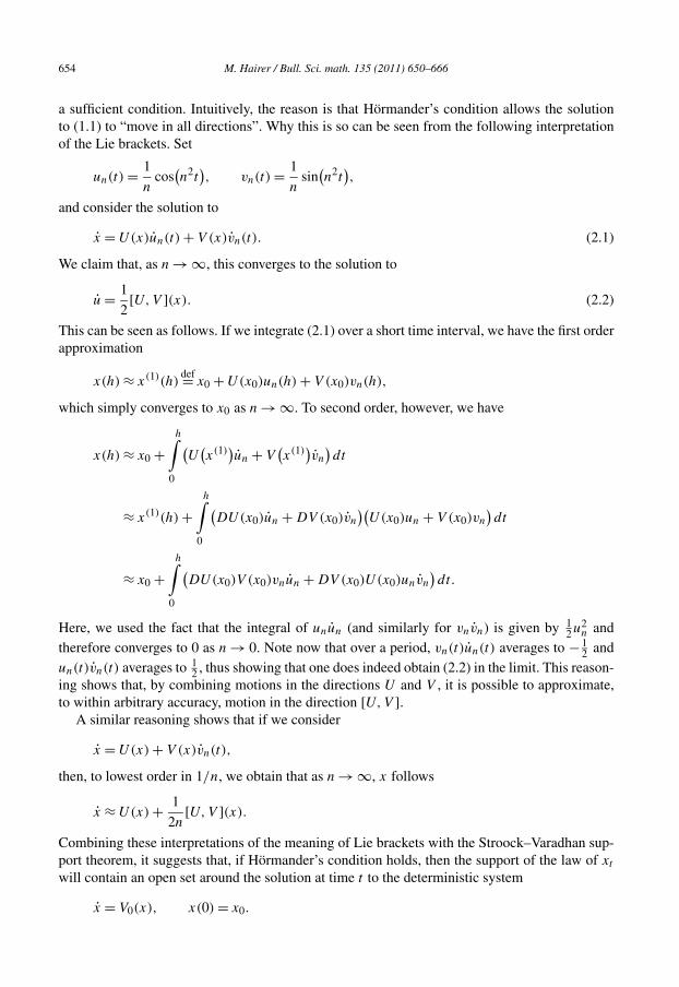
a sufficient condition. Intuitively, the reason is that Hörmander’s condition allows the solutionto (1.1) to “move in all directions”. Why this is so can be seen from the following interpretationof the Lie brackets. Set
un(t) = 1
ncos
(n2t
), vn(t) = 1
nsin
(n2t
),
and consider the solution to
x = U(x)un(t) + V (x)vn(t). (2.1)
We claim that, as n → ∞, this converges to the solution to
u = 1
2[U,V ](x). (2.2)
This can be seen as follows. If we integrate (2.1) over a short time interval, we have the first orderapproximation
x(h) ≈ x(1)(h)def= x0 + U(x0)un(h) + V (x0)vn(h),
which simply converges to x0 as n → ∞. To second order, however, we have
x(h) ≈ x0 +h∫
0
(U
(x(1)
)un + V
(x(1)
)vn
)dt
≈ x(1)(h) +h∫
0
(DU(x0)un + DV (x0)vn
)(U(x0)un + V (x0)vn
)dt
≈ x0 +h∫
0
(DU(x0)V (x0)vnun + DV (x0)U(x0)unvn
)dt.
Here, we used the fact that the integral of unun (and similarly for vnvn) is given by 12u2
n andtherefore converges to 0 as n → 0. Note now that over a period, vn(t)un(t) averages to − 1
2 andun(t)vn(t) averages to 1
2 , thus showing that one does indeed obtain (2.2) in the limit. This reason-ing shows that, by combining motions in the directions U and V , it is possible to approximate,to within arbitrary accuracy, motion in the direction [U,V ].
A similar reasoning shows that if we consider
x = U(x) + V (x)vn(t),
then, to lowest order in 1/n, we obtain that as n → ∞, x follows
x ≈ U(x) + 1
2n[U,V ](x).
Combining these interpretations of the meaning of Lie brackets with the Stroock–Varadhan sup-port theorem, it suggests that, if Hörmander’s condition holds, then the support of the law of xt
will contain an open set around the solution at time t to the deterministic system
x = V0(x), x(0) = x0.
M. Hairer / Bull. Sci. math. 135 (2011) 650–666 655
This should at least render it plausible that under these conditions, the law of xt has a density withrespect to Lebesgue measure. The aim of this note is to demonstrate how to turn this heuristicreasoning into a mathematical theorem with, hopefully, only a minimal amount of effort.
Remark 2.2. While Hörmander’s condition implies that the control system associated to (1.1)reaches an open set around the solution to the deterministic equation x = V0(x), it does not implyin general that it can reach an open set around x0. In particular, it is not true that the parabolicHörmander condition implies that (1.1) can reach every open set. A standard counterexample isgiven by
dx = − sin(x) dt + cos(x) ◦ dW(t), x0 = 0,
which satisfies Hörmander’s condition but can never exit the interval [−π/2,π/2].
3. An introduction to Malliavin calculus
In this section, we collect a number of tools that will be needed in the proof. The main tool isthe integration by parts formula from Malliavin calculus, as well of course as Malliavin calculusitself.
The main tool in the proof is the Malliavin calculus with its integration by part formula inWiener space, which was developed precisely in order to provide a probabilistic proof of The-orem 1.3. It essentially relies on the fact that the image of a Gaussian measure under a smoothsubmersion that is sufficiently integrable possesses a smooth density with respect to Lebesguemeasure. This can be shown in the following way. First, one observes the following fact:
Lemma 3.1. Let μ be a probability measure on Rn such that the bound∣∣∣∣∫
Rn
D(k)G(x)μ(dx)
∣∣∣∣ � Ck‖G‖∞,
holds for every smooth bounded function G and every k � 1. Then μ has a smooth density withrespect to Lebesgue measure.
Proof. Let s > n/2 so that Hs ⊂ Cb by Sobolev embedding. By duality, the assumption thenimplies that every distributional derivative of μ belongs to the Sobolev space H−s , so that μ
belongs to H� for every � ∈ R. The result then follows from the fact that H� ⊂ Ck as soon as� > k + n
2 . �Consider now a sequence of N independent Gaussian random variables δwk with variances
δtk for k ∈ {1, . . . ,N}, as well as a smooth map X: RN → Rn. We also denote by w the collection{δwk}k�1 and we define the n × n matrix-valued map
Mij (w) =∑
k
∂kXi(w)∂kXj (w)δtk, (3.1)
where we use ∂k as a shorthand for the partial derivative with respect to the variable δwk . Withthis notation, X being a submersion is equivalent to M (w) being invertible for every w.
Before we proceed, let us introduce additional notation, which hints at the fact that one wouldreally like to interpret the δwk as the increments of a Wiener process of an interval of length δtk .
656 M. Hairer / Bull. Sci. math. 135 (2011) 650–666
When considering a family {Fk}Nk=1 of maps from RN → Rn, we identify it with a continuousfamily {Ft }t�0, where
Ftdef= Fk, t ∈ [tk, tk+1), tk
def=∑��k
δt�. (3.2)
Note that with this convention, we have t0 = 0, t1 = δt1, etc. This is of course an abuse of notationsince Ft is not equal to Fk for t = k, but we hope that it will always be clear from the contextwhether the index is a discrete or a continuous variable. We also set Ft = 0 for t � tN . With thisnotation, we have the natural identity∫
Ft dt =N∑
k=1
Fkδtk.
Furthermore, given a smooth map G: RN → R, we will from now on denote by DtG the familyof maps such that DtG = ∂kG for t ∈ [tk, tk+1), so that (3.1) can be rewritten as
Mij (w) =∫
DtXi(w)DtXj (w)dt.
The quantity DtG is called the Malliavin derivative of the random variable G.The main feature of the Malliavin derivative operator Dt suggesting that one expects it to
be well-posed in the limit N → ∞ is that it was set up in such a way that it is invariant underrefinement of the mesh {δtk} in the following way. For every k, set δwk = δw−
k + δw+k , where
δw±k are independent Gaussians with variances δt±k with δt−k + δt+k = δtk and then identify maps
G: RN → R with a map G: R2N → R by
G(δw±
1 , . . . , δw±N
) = G(δw−
1 + δw+1 , . . . , δw−
N + δw+N
).
Then, for every t � 0, Dt G is precisely the map identified with DtG.With all of these notations at hand, we then have the following result:
Theorem 3.2. Let X: RN → Rn be smooth, assume that M (w) is invertible for every w and that,for every p > 1 and every m � 0, we have
E∣∣∂k1 · · · ∂kmXi(w)
∣∣p < ∞, E∥∥M (w)−1
∥∥p< ∞. (3.3)
Then the law of X(w) has a smooth density with respect to Lebesgue measure. Furthermore,the derivatives of the law of X can be bounded from above by expressions that depend only onthe bounds (3.3), but are independent of N , provided that
∑δtk = T remains fixed.
Before we turn to the proof of this result, we perform a few preliminary calculations. BesidesLemma 3.1, the main ingredient of the proof of Theorem 3.2 will be the following integration byparts formula which lies at the heart of the success of Malliavin calculus. If Fk and G are squareintegrable functions with square integrable derivatives, then we have the identity
E( ∫
DtG(w)Ft (w)dt
)= E
∑k
∂kG(w)Fk(w)δtk
= EG(w)∑
k
Fk(w)δwk − EG(w)∑
k
∂kFk(w)δtk
def= E(
G(w)
∫Ft dw(t)
), (3.4)
M. Hairer / Bull. Sci. math. 135 (2011) 650–666 657
where we defined the Skorokhod integral∫
Ft dw(t) by the expression on the second line. Notethat in order to obtain (3.4), we only integrated by parts with respect to the variables δwk .
Remark 3.3. The Skorokhod integral is really an extension of the usual Itô integral, which is thejustification for our notation. This is because, if Ft is an adapted process, then Ftk is independentof δw� for � � k by definition. As a consequence, the term ∂kFk drops and we are reduced to theusual Itô integral.
Remark 3.4. It follows immediately from the definition that one has the identity
Dt
∫Fs dw(s) = Ft +
∫DtFs dw(s). (3.5)
Formally, one can think of this identity as being derived from the Leibnitz rule, combined with theidentity Dt (dw(s)) = δ(t − s) ds, which is a kind of continuous analogue of the trivial discreteidentity ∂kδw� = δk�.
This Skorokhod integral satisfies the following extension of Itô’s isometry:
Proposition 3.5. Let Fk be square integrable functions with square integrable derivatives, then
E( ∫
Ft dw(t)
)2
= E∫
F 2t (w)dt + E
∫∫DtFs(w)DtFs(w)ds dt
� E∫
F 2t (w)dt + E
∫∫ ∣∣DtFs(w)∣∣2
ds dt,
holds.
Proof. It follows from the definition that one has the identity
E( ∫
Ft dw(t)
)2
=∑k,�
E(FkF�δwkδw� + ∂kFk∂�F�δtkδt� − 2Fk∂�F�δwkδt�).
Applying the identity EGδw� = E∂�Gδt� to the first term in the above formula (with G =FkF�δwk), we thus obtain
· · · =∑k,�
E(FkF�δk,�δt� + ∂kFk∂�F�δtkδt� + (F�∂�Fk − Fk∂�F�)δwkδt�
).
Applying the same identity to the last term then finally leads to
· · · =∑k,�
E(FkF�δk,�δt� + ∂kF�∂�Fkδtkδt�),
which is precisely the desired result. �As a consequence, we have the following:
Proposition 3.6. Assume that∑
δtk = T < ∞. Then, for every p > 0 there exist C > 0 andk > 0 such that the bound
658 M. Hairer / Bull. Sci. math. 135 (2011) 650–666
E
∣∣∣∣∫
Fs dw(s)
∣∣∣∣p
� C
(1 +
∑0���k
supt0,...,t�
E|Dt1 · · ·Dt�Ft0 |2p
),
holds. Here, C may depend on T and p, but k depends only on p.
Proof. Since the case p � 2 follows from Proposition 3.5, we can assume without loss of gen-erality that p > 2. Combining (3.4) with (3.5) and then applying Hölder’s inequality, we have
E
∣∣∣∣∫
Fs dw(s)
∣∣∣∣p
= (p − 1)E
∣∣∣∣∫
Fs dw(s)
∣∣∣∣p−2 ∫
Ft
(Ft +
∫DtFs dw(s)
)dt
� 1
2E
∣∣∣∣∫
Fs dw(s)
∣∣∣∣p
+ cE∫ ∣∣∣∣Ft +
∫DtFs dw(s)
∣∣∣∣2p3
dt + cE∫
|Ft |2p dt
� 1
2E
∣∣∣∣∫
Fs dw(s)
∣∣∣∣p
+ cE∫ ∣∣∣∣
∫DtFs dw(s)
∣∣∣∣2p3
dt + cE∫ (
1 + |Ft |)2p
dt,
where c is some constant depending on p and T that changes from line to line. The claim nowfollows by induction. �Remark 3.7. The bound in Proposition 3.6 is clearly very far from optimal. Actually, it is knownthat, for every p � 1, there exists C such that
E
∣∣∣∣∫
Fs dw(s)
∣∣∣∣2p
� CE
∣∣∣∣∫
F 2s ds
∣∣∣∣p
+ CE
∣∣∣∣∫
|DtFs |2 ds dt
∣∣∣∣p
,
even if T = ∞. However, this extension of the Burkholder–Davies–Gundy inequality requireshighly non-trivial harmonic analysis and, to best of the author’s knowledge, cannot be reduced toa short elementary calculation. The reader interested in knowing more can find its proof in [21,Chapters 1.3–1.5].
The proof of Theorem 3.2 is now straightforward:
Proof of Theorem 3.2. We want to show that Lemma 3.1 can be applied. From the definitionof M , we have for every j the identity
(DjG)(X(w)
) =∑k,m
∂k
(G
(X(w)
))∂kXm(w)δtkM
−1mj (w). (3.6)
Combining this identity with (3.4), it follows that
EDjG(X) = E(
G(X(w)
)∑m
∫DtXm(w)M −1
mj (w)dw(t)
). (3.7)
Note that, by the chain rule, one has the identity
DtM−1 = −M −1(DtM )M −1,
and similarly for higher order derivatives, so that the Malliavin derivatives of M −1 can bebounded by terms involving M −1 and the Malliavin derivatives of X.
M. Hairer / Bull. Sci. math. 135 (2011) 650–666 659
Combining this with Proposition 3.5 and (3.3) immediately shows that the requested resultholds for k = 1. Higher values of k can be treated by induction by repeatedly applying (3.6).This will lead to expressions of the type (3.7), with the right-hand side consisting of multipleSkorokhod integrals of higher order polynomials in M −1 and derivatives of X.
By Proposition 3.6, the moments of each of the terms appearing in this way can be boundedby finitely many of the expressions appearing in the assumption so that the required statementfollows. �4. Application to diffusion processes
We are now almost ready to tackle the proof of Hörmander’s theorem. Before we start, wediscuss how DsXt can be computed when Xt is the solution to an SDE of the type (1.1) and weuse this discussion to formulate precise assumption for our theorem.
4.1. Malliavin calculus for diffusion processes
By taking the limit N → ∞ and δtk → 0 with∑
δtk = 1, the results in the previous sec-tion show that one can define a “Malliavin derivative” operator D , acting on a suitable class of“smooth” random variables and returning a stochastic process that has all the usual properties ofa derivative. Let us see how it acts on the solution to an SDE of the type (1.1).
An important tool for our analysis will be the linearisation of (1.1) with respect to its initialcondition. Denote by Φt the (random) solution map to (1.1), so that xt = Φt(x0). It is thenknown that, under Assumption 4.2 below, Φt is almost surely a smooth map for every t . Weactually obtain a flow of smooth maps, namely a two-parameter family of maps Φs,t such thatxt = Φs,t (xs) for every s � t and such that Φt,u ◦ Φs,t = Φs,u and Φt = Φ0,t . For a given initialcondition x0, we then denote by Js,t the derivative of Φs,t evaluated at xs . Note that the chainrule immediately implies that one has the composition law Js,u = Jt,uJs,t , where the product isgiven by simple matrix multiplication. We also use the notation J
(k)s,t for the kth-order derivative
of Φs,t .It is straightforward to obtain an equation governing J0,t by differentiating both sides of (1.1)
with respect to x0. This yields the non-autonomous linear equation
dJ0,t = DV0(xt )J0,t dt +m∑
i=1
DVi(xt )J0,t ◦ dWi(t), J0,0 = I, (4.1)
where I is the n × n identity matrix. Higher order derivatives J(k)0,t with respect to the initial
condition can be defined similarly.
Remark 4.1. For every s > 0, the quantity Js,t solves the same equation as (4.1), except for theinitial condition which is given by Js,s = I .
On the other hand, we can use (3.5) to, at least on a formal level, take the Malliavin derivativeof the integral form of (1.1), which then yields for r � t the identity
Djr X(t) =
t∫DV0(Xs)D
jr Xs ds +
m∑ t∫DVi(Xs)D
jr Xs ◦ dWi(s) + Vj (Xr).
r i=1 r
660 M. Hairer / Bull. Sci. math. 135 (2011) 650–666
(Here we denote by Dj the Malliavin derivative with respect to Wj ; the generalisation of thediscussion of the previous section to the case of finitely many independent Wiener processes isstraightforward.) We see that, save for the initial condition at time t = r given by Vj (Xr), thisequation is identical to the integral form of (4.1)!
As a consequence, we have for s < t the identity
Djs Xt = Js,tVj (Xs). (4.2)
Furthermore, since Xt is independent of the later increments of W , we have Djs Xt = 0 for
s � t .By the composition property J0,t = Js,tJ0,s , we can write Js,t = J0,t J
−10,s , which will be useful
in the sequel. Here, the inverse J−10,t of the Jacobian can be found by solving the SDE
dJ−10,t = −J−1
0,t DV0(x) dt −m∑
i=1
J−10,t DVi(x) ◦ dWi. (4.3)
This follows from the chain rule by noting that if we denote by Ψ (A) = A−1 the map that takesthe inverse of a square matrix, then we have DΨ (A)H = −A−1HA−1.
This discussion is the motivation for the following assumption, which we assume to be inforce from now on:
Assumption 4.2. The vector fields Vi are C∞ and all of their derivatives grow at most polynomi-ally at infinity. Furthermore, they are such that the solutions to (1.1), (4.1) and (4.3) satisfy
E supt�T
|xt |p < ∞, E supt�T
∣∣J (k)0,t
∣∣p < ∞, E supt�T
∣∣J−10,t
∣∣p < ∞,
for every initial condition x0 ∈ Rn, every terminal time T > 0, every k > 0, and every p > 0.
Remark 4.3. It is well known that Assumption 4.2 holds if the Vi are bounded with boundedderivatives of all orders. However, this is far from being a necessary assumption.
Remark 4.4. Under Assumption 4.2, standard limiting procedures allow to justify (4.2), as wellas all the formal manipulations that we will perform in the sequel.
With these assumptions in place, the version of Hörmander’s theorem that we are going toprove in these notes is as follows:
Theorem 4.5. Let x0 ∈ Rn and let xt be the solution to (1.1). If the vector fields {Vj } satisfy theparabolic Hörmander condition and Assumption 4.2 is satisfied, then the law of Xt has a smoothdensity with respect to Lebesgue measure.
Proof. Denote by A0,t the operator A0,t v = ∫ t
0 Js,tV (Xs)v(s) ds, where v is a square integrable,not necessarily adapted, Rm-valued stochastic process and V is the n×m matrix-valued functionobtained by concatenating the vector fields Vj for j = 1, . . . ,m. With this notation, it followsfrom (4.2) that the Malliavin covariance matrix M0,t of Xt is given by
M0,t = A0,tA∗
0,t =t∫Js,tV (Xs)V
∗(Xs)J∗s,t ds.
0
M. Hairer / Bull. Sci. math. 135 (2011) 650–666 661
It follows from (4.2) that the assumptions of Theorem 3.2 are satisfied for the random variable Xt ,provided that we can show that ‖M −1
0,t ‖ has bounded moments of all orders. This in turn followsby combining Lemma 4.7 with Theorem 4.8 below. �4.2. Proof of Hörmander’s theorem
The remainder of this section is devoted to a proof of the fact that Hörmander’s condition issufficient to guarantee the invertibility of the Malliavin matrix of a diffusion process. For purelytechnical reasons, it turns out to be advantageous to rewrite the Malliavin matrix as
M0,t = J0,tC0,t J∗0,t , C0,t =
t∫0
J−10,s V (Xs)V
∗(Xs)(J−1
0,s
)∗ds,
where C0,t is the reduced Malliavin matrix of our diffusion process.
Remark 4.6. The reason for considering the reduced Malliavin matrix is that the process appear-ing under the integral in the definition of C0,t is adapted to the filtration generated by Wt . Thisallows us to use some tools from stochastic calculus that would not be available otherwise.
Since we assumed that J0,t has inverse moments of all orders, the invertibility of M0,t isequivalent to that of C0,t . Note first that since C0,t is a positive definite symmetric matrix,the norm of its inverse is given by
∥∥C −10,t
∥∥ =(
inf|η|=1〈η,C0,t η〉
)−1.
A very useful observation is then the following:
Lemma 4.7. Let M be a symmetric positive semidefinite n × n matrix-valued random variablesuch that E‖M‖p < ∞ for every p � 1 and such that, for every p � 1 there exists Cp such that
sup|η|=1
P(〈η,Mη〉 < ε
)� Cpεp, (4.4)
holds for every ε � 1. Then, E‖M−1‖p < ∞ for every p � 1.
Proof. The non-trivial part of the result is that the supremum over η is taken outside of theprobability in (4.4). For ε > 0, let {ηk}k�N be a sequence of vectors with |ηk| = 1 such that forevery η with |η| � 1, there exists k such that |ηk − η| � ε2. It is clear that one can find such a setwith N � Cε2−2n for some C > 0 independent of ε. We then have the bound
〈η,Mη〉 = 〈ηk,Mηk〉 + 〈η − ηk,Mη〉 + 〈η − ηk,Mηk〉� 〈ηk,Mηk〉 − 2‖M‖ε2,
so that
P(
inf|η|=1〈η,Mη〉 � ε
)� P
(inf
k�N〈ηk,Mηk〉 � 4ε
)+ P
(‖M‖ � 1
ε
)
� Cε2−2n sup P(〈η,Mη〉 � 4ε
) + P(
‖M‖ � 1
ε
).
|η|=1
662 M. Hairer / Bull. Sci. math. 135 (2011) 650–666
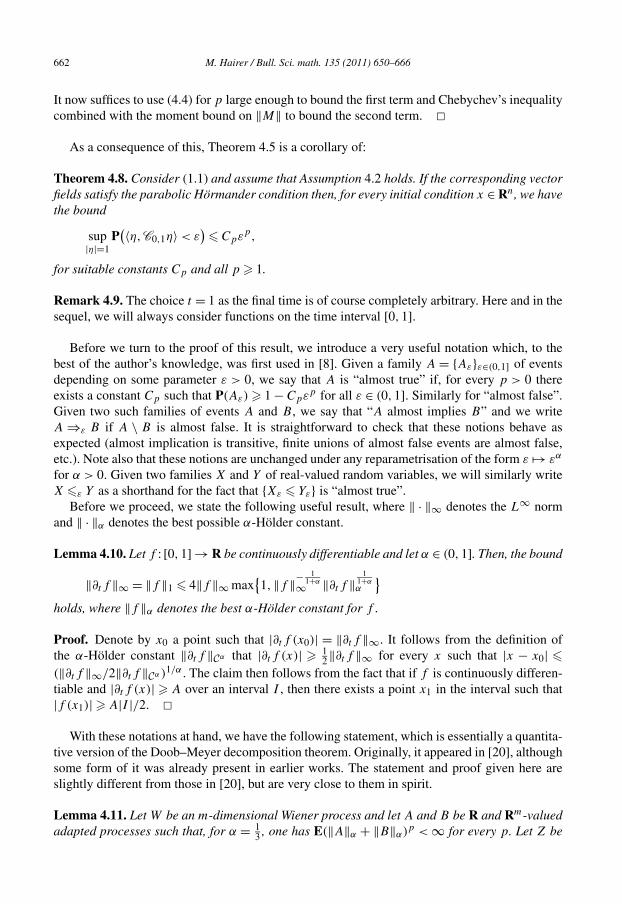
It now suffices to use (4.4) for p large enough to bound the first term and Chebychev’s inequalitycombined with the moment bound on ‖M‖ to bound the second term. �
As a consequence of this, Theorem 4.5 is a corollary of:
Theorem 4.8. Consider (1.1) and assume that Assumption 4.2 holds. If the corresponding vectorfields satisfy the parabolic Hörmander condition then, for every initial condition x ∈ Rn, we havethe bound
sup|η|=1
P(〈η,C0,1η〉 < ε
)� Cpεp,
for suitable constants Cp and all p � 1.
Remark 4.9. The choice t = 1 as the final time is of course completely arbitrary. Here and in thesequel, we will always consider functions on the time interval [0,1].
Before we turn to the proof of this result, we introduce a very useful notation which, to thebest of the author’s knowledge, was first used in [8]. Given a family A = {Aε}ε∈(0,1] of eventsdepending on some parameter ε > 0, we say that A is “almost true” if, for every p > 0 thereexists a constant Cp such that P(Aε) � 1 − Cpεp for all ε ∈ (0,1]. Similarly for “almost false”.Given two such families of events A and B , we say that “A almost implies B” and we writeA ⇒ε B if A \ B is almost false. It is straightforward to check that these notions behave asexpected (almost implication is transitive, finite unions of almost false events are almost false,etc.). Note also that these notions are unchanged under any reparametrisation of the form ε �→ εα
for α > 0. Given two families X and Y of real-valued random variables, we will similarly writeX �ε Y as a shorthand for the fact that {Xε � Yε} is “almost true”.
Before we proceed, we state the following useful result, where ‖ · ‖∞ denotes the L∞ normand ‖ · ‖α denotes the best possible α-Hölder constant.
Lemma 4.10. Let f : [0,1] → R be continuously differentiable and let α ∈ (0,1]. Then, the bound
‖∂tf ‖∞ = ‖f ‖1 � 4‖f ‖∞ max{1,‖f ‖− 1
1+α∞ ‖∂tf ‖1
1+αα
}holds, where ‖f ‖α denotes the best α-Hölder constant for f .
Proof. Denote by x0 a point such that |∂tf (x0)| = ‖∂tf ‖∞. It follows from the definition ofthe α-Hölder constant ‖∂tf ‖Cα that |∂tf (x)| � 1
2‖∂tf ‖∞ for every x such that |x − x0| �(‖∂tf ‖∞/2‖∂tf ‖Cα )1/α . The claim then follows from the fact that if f is continuously differen-tiable and |∂tf (x)| � A over an interval I , then there exists a point x1 in the interval such that|f (x1)| � A|I |/2. �
With these notations at hand, we have the following statement, which is essentially a quantita-tive version of the Doob–Meyer decomposition theorem. Originally, it appeared in [20], althoughsome form of it was already present in earlier works. The statement and proof given here areslightly different from those in [20], but are very close to them in spirit.
Lemma 4.11. Let W be an m-dimensional Wiener process and let A and B be R and Rm-valuedadapted processes such that, for α = 1 , one has E(‖A‖α + ‖B‖α)p < ∞ for every p. Let Z be
3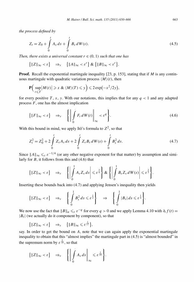
M. Hairer / Bull. Sci. math. 135 (2011) 650–666 663
the process defined by
Zt = Z0 +t∫
0
As ds +t∫
0
Bs dW(s). (4.5)
Then, there exists a universal constant r ∈ (0,1) such that one has{‖Z‖∞ < ε} ⇒ε
{‖A‖∞ < εr}
&{‖B‖∞ < εr
}.
Proof. Recall the exponential martingale inequality [23, p. 153], stating that if M is any contin-uous martingale with quadratic variation process 〈M〉(t), then
P(
supt�T
∣∣M(t)∣∣ � x & 〈M〉(T ) � y
)� 2 exp
(−x2/2y),
for every positive T , x, y. With our notations, this implies that for any q < 1 and any adaptedprocess F , one has the almost implication
{‖F‖∞ < ε} ⇒ε
{∥∥∥∥∥·∫
0
Ft dW(t)
∥∥∥∥∥∞< εq
}. (4.6)
With this bound in mind, we apply Itô’s formula to Z2, so that
Z2t = Z2
0 + 2
t∫0
ZsAs ds + 2
t∫0
ZsBs dW(s) +t∫
0
B2s ds. (4.7)
Since ‖A‖∞ �ε ε−1/4 (or any other negative exponent for that matter) by assumption and simi-larly for B , it follows from this and (4.6) that
{‖Z‖∞ < ε} ⇒ε
{∣∣∣∣∣1∫
0
AsZs ds
∣∣∣∣∣ � ε34
}&
{∣∣∣∣∣1∫
0
BsZs dW(s)
∣∣∣∣∣ � ε23
}.
Inserting these bounds back into (4.7) and applying Jensen’s inequality then yields
{‖Z‖∞ < ε} ⇒ε
{ 1∫0
B2s ds � ε
12
}⇒
{ 1∫0
|Bs |ds � ε14
}.
We now use the fact that ‖B‖α �ε ε−q for every q > 0 and we apply Lemma 4.10 with ∂tf (t) =|Bt | (we actually do it component by component), so that{‖Z‖∞ < ε
} ⇒ε
{‖B‖∞ � ε117
},
say. In order to get the bound on A, note that we can again apply the exponential martingaleinequality to obtain that this “almost implies” the martingale part in (4.5) is “almost bounded” in
the supremum norm by ε118 , so that
{‖Z‖∞ < ε} ⇒ε
{∥∥∥∥∥·∫As ds
∥∥∥∥∥∞� ε
118
}.
0
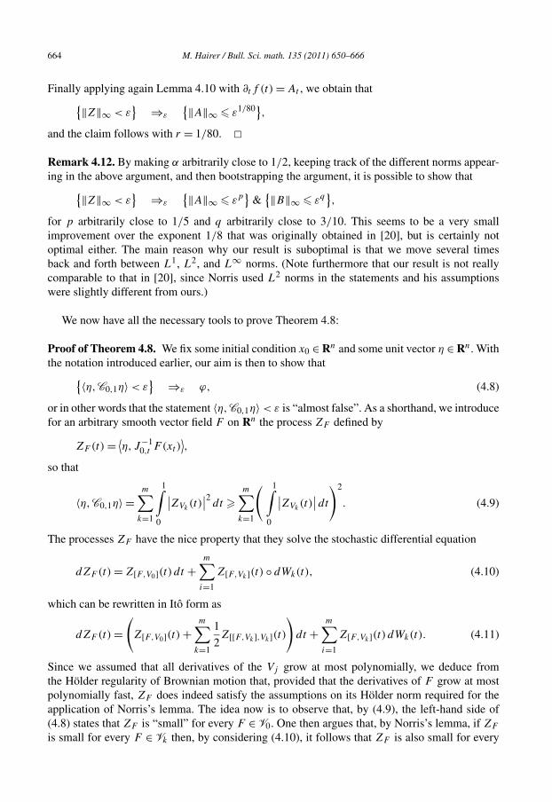
664 M. Hairer / Bull. Sci. math. 135 (2011) 650–666
Finally applying again Lemma 4.10 with ∂tf (t) = At , we obtain that{‖Z‖∞ < ε} ⇒ε
{‖A‖∞ � ε1/80},and the claim follows with r = 1/80. �Remark 4.12. By making α arbitrarily close to 1/2, keeping track of the different norms appear-ing in the above argument, and then bootstrapping the argument, it is possible to show that{‖Z‖∞ < ε
} ⇒ε
{‖A‖∞ � εp}
&{‖B‖∞ � εq
},
for p arbitrarily close to 1/5 and q arbitrarily close to 3/10. This seems to be a very smallimprovement over the exponent 1/8 that was originally obtained in [20], but is certainly notoptimal either. The main reason why our result is suboptimal is that we move several timesback and forth between L1, L2, and L∞ norms. (Note furthermore that our result is not reallycomparable to that in [20], since Norris used L2 norms in the statements and his assumptionswere slightly different from ours.)
We now have all the necessary tools to prove Theorem 4.8:
Proof of Theorem 4.8. We fix some initial condition x0 ∈ Rn and some unit vector η ∈ Rn. Withthe notation introduced earlier, our aim is then to show that{〈η,C0,1η〉 < ε
} ⇒ε ϕ, (4.8)
or in other words that the statement 〈η,C0,1η〉 < ε is “almost false”. As a shorthand, we introducefor an arbitrary smooth vector field F on Rn the process ZF defined by
ZF (t) = ⟨η,J−1
0,t F (xt )⟩,
so that
〈η,C0,1η〉 =m∑
k=1
1∫0
∣∣ZVk(t)
∣∣2dt �
m∑k=1
( 1∫0
∣∣ZVk(t)
∣∣dt
)2
. (4.9)
The processes ZF have the nice property that they solve the stochastic differential equation
dZF (t) = Z[F,V0](t) dt +m∑
i=1
Z[F,Vk](t) ◦ dWk(t), (4.10)
which can be rewritten in Itô form as
dZF (t) =(
Z[F,V0](t) +m∑
k=1
1
2Z[[F,Vk],Vk](t)
)dt +
m∑i=1
Z[F,Vk](t) dWk(t). (4.11)
Since we assumed that all derivatives of the Vj grow at most polynomially, we deduce fromthe Hölder regularity of Brownian motion that, provided that the derivatives of F grow at mostpolynomially fast, ZF does indeed satisfy the assumptions on its Hölder norm required for theapplication of Norris’s lemma. The idea now is to observe that, by (4.9), the left-hand side of(4.8) states that ZF is “small” for every F ∈ V0. One then argues that, by Norris’s lemma, if ZF
is small for every F ∈ Vk then, by considering (4.10), it follows that ZF is also small for every
M. Hairer / Bull. Sci. math. 135 (2011) 650–666 665
F ∈ Vk+1. Hörmander’s condition then ensures that a contradiction arises at some stage, sinceZF (0) = 〈F(x0), ξ 〉 and there exists k such that Vk(x0) spans all of Rn.
Let us make this rigorous. It follows from Norris’s lemma and (4.11) that one has the almostimplication{‖ZF ‖∞ < ε
} ⇒ε
{‖Z[F,Vk]‖∞ < εr}
&{‖ZG‖∞ < εr
},
for k = 1, . . . ,m and for G = [F,V0]+ 12
∑mk=1[[F,Vk],Vk]. Iterating this bound a second time,
this time considering the equation for ZG, we obtain that{‖ZF ‖∞ < ε} ⇒ε
{‖Z[[F,Vk],V�]‖∞ < εr2},
so that we finally obtain the implication{‖ZF ‖∞ < ε} ⇒ε
{‖Z[F,Vk]‖∞ < εr2}, (4.12)
for k = 0, . . . ,m.At this stage, we are basically done. Indeed, combining (4.9) with Lemma 4.10 as above, we
see that{〈η,C0,1η〉 < ε} ⇒ε
{‖ZVk‖∞ < ε1/5}.
Applying (4.12) iteratively, we see that for every k > 0 there exists some qk > 0 such that{〈η,C0,1η〉 < ε} ⇒ε
⋂V ∈Vk
{‖ZV ‖∞ < εqk}.
Since ZV (0) = 〈η,V (x0)〉 and since there exists some k > 0 such that Vk(x0) = Rn, the right-hand side of this expression is empty for some sufficiently large value of k, which is preciselythe desired result. �Acknowledgements
These notes were part of a minicourse given at the University of Warwick in July 2010; thanksare due to the organisers for this pleasant event. I would also like to thank Michael Scheutzow andHendrik Weber who carefully read a previous version of the manuscript and pointed out severalmisprints. Remaining mistakes were probably added later on! Finally, I would like to acknowl-edge financial support provided by the EPSRC through grants EP/E002269/1 and EP/D071593/1,the Royal Society through a Wolfson Research Merit Award, and the Leverhulme Trust througha Philip Leverhulme prize.
References
[1] F. Baudoin, M. Hairer, A version of Hörmander’s theorem for the fractional Brownian motion, Probab. TheoryRelated Fields 139 (3–4) (2007) 373–395.
[2] J.-M. Bismut, Martingales, the Malliavin calculus and Hörmander’s theorem, in: Stochastic Integrals, Proc. Sym-pos., Univ. Durham, Durham, 1980, in: Lecture Notes in Math., vol. 851, Springer, Berlin, 1981, pp. 85–109.
[3] J.-M. Bismut, Martingales, the Malliavin calculus and hypoellipticity under general Hörmander’s conditions,Z. Wahrsch. Verw. Geb. 56 (4) (1981) 469–505.
[4] F. Baudoin, J. Teichmann, Hypoellipticity in infinite dimensions and an application in interest rate theory, Ann.Appl. Probab. 15 (3) (2005) 1765–1777.
[5] T. Cass, Smooth densities for solutions to stochastic differential equations with jumps, Stochastic Process.Appl. 119 (5) (2009) 1416–1435.
666 M. Hairer / Bull. Sci. math. 135 (2011) 650–666
[6] T. Cass, P. Friz, Densities for rough differential equations under Hörmander’s condition, Ann. of Math. (2) 171 (3)(2010) 2115–2141.
[7] M. Hairer, J.C. Mattingly, Ergodicity of the 2D Navier–Stokes equations with degenerate stochastic forcing, Ann.of Math. (2) 164 (3) (2006) 993–1032.
[8] M. Hairer, J.C. Mattingly, A theory of hypoellipticity and unique ergodicity for semilinear stochastic PDEs, Elec-tron. J. Probab. 16 (2011) 658–738.
[9] B. Helffer, F. Nier, Hypoelliptic Estimates and Spectral Theory for Fokker–Planck Operators and Witten Laplacians,Lecture Notes in Math., vol. 1862, Springer-Verlag, Berlin, 2005.
[10] L. Hörmander, Hypoelliptic second order differential equations, Acta Math. 119 (1967) 147–171.[11] L. Hörmander, The Analysis of Linear Partial Differential Operators I–IV, Springer, New York, 1985.[12] M. Hairer, N. Pillai, Ergodicity of hypoelliptic SDEs driven by fractional Brownian motion, Ann. Inst. H. Poincaré
Probab. Statist. 47 (2) (2011) 601–628.[13] Y. Ishikawa, H. Kunita, Malliavin calculus on the Wiener–Poisson space and its application to canonical SDE with
jumps, Stochastic Process. Appl. 116 (12) (2006) 1743–1769.[14] J.J. Kohn, Lectures on degenerate elliptic problems, in: Pseudodifferential Operator with Applications, Bressanone,
1977, Liguori, Naples, 1978, pp. 89–151.[15] S. Kusuoka, D. Stroock, Applications of the Malliavin calculus. I, in: Stochastic Analysis, Katata/Kyoto, 1982, in:
North-Holland Math. Library, vol. 32, North-Holland, Amsterdam, 1984, pp. 271–306.[16] S. Kusuoka, D. Stroock, Applications of the Malliavin calculus. II, J. Fac. Sci. Univ. Tokyo Sect. IA Math. 32 (1)
(1985) 1–76.[17] S. Kusuoka, D. Stroock, Applications of the Malliavin calculus. III, J. Fac. Sci. Univ. Tokyo Sect. IA Math. 34 (2)
(1987) 391–442.[18] P. Malliavin, Stochastic calculus of variations and hypoelliptic operators, in: Proc. Intern. Symp. SDE, Kinokunia,
Kyoto, 1976, pp. 195–263.[19] J.C. Mattingly, É. Pardoux, Malliavin calculus for the stochastic 2D Navier–Stokes equation, Comm. Pure Appl.
Math. 59 (12) (2006) 1742–1790.[20] J. Norris, Simplified Malliavin calculus, in: Séminaire de Probabilités, XX, 1984/1985, in: Lecture Notes in Math.,
vol. 1204, Springer, Berlin, 1986, pp. 101–130.[21] D. Nualart, The Malliavin Calculus and Related Topics, Probab. Appl. (N. Y.), Springer-Verlag, New York, 1995.[22] D. Ocone, Stochastic calculus of variations for stochastic partial differential equations, J. Funct. Anal. 79 (2) (1988)
288–331.[23] D. Revuz, M. Yor, Continuous Martingales and Brownian Motion, third ed., Grundlehren Math. Wiss., vol. 293,
Springer-Verlag, Berlin, 1999.[24] D.W. Stroock, S.R.S. Varadhan, On the support of diffusion processes with applications to the strong maximum
principle, in: Proceedings of the Sixth Berkeley Symposium on Mathematical Statistics and Probability, Univ.California, Berkeley, CA, 1970/1971, vol. III: Probability Theory, Univ. California Press, Berkeley, CA, 1972,pp. 333–359.
[25] A. Takeuchi, The Malliavin calculus for SDE with jumps and the partially hypoelliptic problem, OsakaJ. Math. 39 (3) (2002) 523–559.
[26] A. Takeuchi, Bismut–Elworthy–Li-type formulae for stochastic differential equations with jumps, J. Theoret.Probab. 23 (2010) 576–604.