On metamodelling of wheel-rail contact in S&C

Rostyslav Skrypnyk – rostyslav.skrypnyk@chalmers.se,Jens Nielsen, Magnus Ekh, Jim BrouzoulisSeptember 14-15, 2016 @NSRT

Chalmers University of Technology / CHARMEC

Background

Motivation

Sweden per annum200-300 millions SEK

(20 % of the overall maintenancecosts)

1/15

Motivation

Sweden per annum

200-300 millions SEK(20 % of the overall maintenance

costs)

1/15

Motivation

Sweden per annum200-300 millions SEK

(20 % of the overall maintenancecosts)

1/15

Background

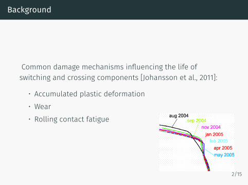
Common damage mechanisms influencing the life ofswitching and crossing components [Johansson et al., 2011]:

• Accumulated plastic deformation• Wear• Rolling contact fatigue

2/15

Background

Common damage mechanisms influencing the life ofswitching and crossing components [Johansson et al., 2011]:

• Accumulated plastic deformation

• Wear• Rolling contact fatigue

2/15

Background

Common damage mechanisms influencing the life ofswitching and crossing components [Johansson et al., 2011]:

• Accumulated plastic deformation• Wear

• Rolling contact fatigue

2/15

Background

Common damage mechanisms influencing the life ofswitching and crossing components [Johansson et al., 2011]:

• Accumulated plastic deformation• Wear• Rolling contact fatigue

2/15

Simulation methodology [Johansson et al., 2011]

vF

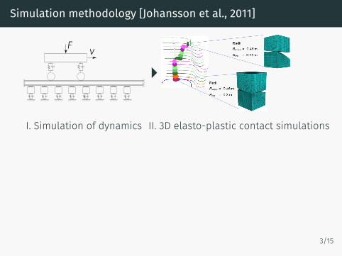
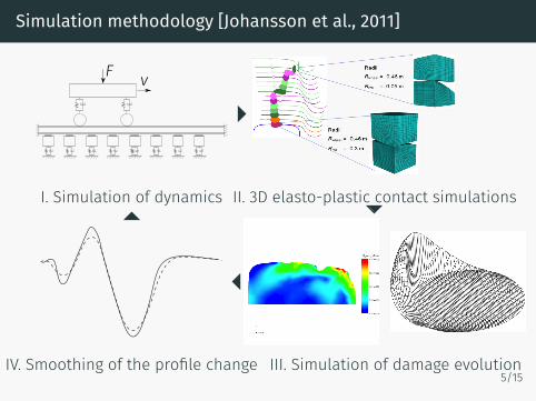
I. Simulation of dynamics II. 3D elasto-plastic contact simulations

III. Simulation of damage evolutionIV. Smoothing of the profile change

3/15

Simulation methodology [Johansson et al., 2011]

vF

I. Simulation of dynamics

II. 3D elasto-plastic contact simulations

III. Simulation of damage evolutionIV. Smoothing of the profile change

3/15

Simulation methodology [Johansson et al., 2011]

vF

I. Simulation of dynamics II. 3D elasto-plastic contact simulations

III. Simulation of damage evolutionIV. Smoothing of the profile change

3/15

Simulation methodology [Johansson et al., 2011]

vF

I. Simulation of dynamics II. 3D elasto-plastic contact simulations

III. Simulation of damage evolution

IV. Smoothing of the profile change

3/15

Simulation methodology [Johansson et al., 2011]

vF

I. Simulation of dynamics II. 3D elasto-plastic contact simulations

III. Simulation of damage evolutionIV. Smoothing of the profile change3/15

Application of methodology in Haste, Germany

Comparison with field measurements:

• Comparison of measured and simulated profiles after fiveweeks of traffic

• Plastic deformation is initially the dominating damagemechanism, later wear dominates

• Good qualitative agreement

4/15

Application of methodology in Haste, Germany

Comparison with field measurements:

• Comparison of measured and simulated profiles after fiveweeks of traffic

• Plastic deformation is initially the dominating damagemechanism, later wear dominates

• Good qualitative agreement

4/15

Application of methodology in Haste, Germany

Comparison with field measurements:

• Comparison of measured and simulated profiles after fiveweeks of traffic

• Plastic deformation is initially the dominating damagemechanism, later wear dominates

• Good qualitative agreement

4/15

Application of methodology in Haste, Germany

Comparison with field measurements:

• Comparison of measured and simulated profiles after fiveweeks of traffic

• Plastic deformation is initially the dominating damagemechanism, later wear dominates

• Good qualitative agreement

4/15

Simulation methodology [Johansson et al., 2011]

vF

I. Simulation of dynamics II. 3D elasto-plastic contact simulations

III. Simulation of damage evolutionIV. Smoothing of the profile change5/15

Simulation methodology [Johansson et al., 2011]

vF

I. Simulation of dynamics II. 3D elasto-plastic contact simulations

III. Simulation of damage evolutionIV. Smoothing of the profile change5/15

3D contact problem

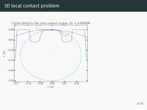
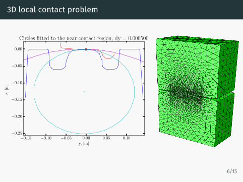
3D local contact problem

−0.15 −0.10 −0.05 0.00 0.05 0.10

y, [m]

−0.25

−0.20

−0.15

−0.10

−0.05

0.00

z,[m

]

Circles fitted to the near contact region, dy = 0.000500

6/15

3D local contact problem

−0.15 −0.10 −0.05 0.00 0.05 0.10

y, [m]

−0.25

−0.20

−0.15

−0.10

−0.05

0.00

z,[m

]

Circles fitted to the near contact region, dy = 0.000500

6/15

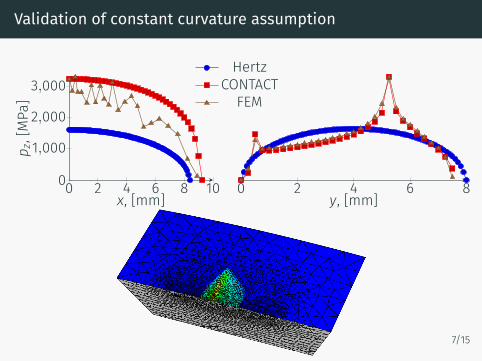
Validation of constant curvature assumption

0 2 4 6 8 100

1,000

2,000

3,000

x, [mm]

p z,[MPa]

HertzCONTACTFEM

0 2 4 6 8y, [mm]

7/15

Metamodel

Definition

Metamodel g is a model of a model, i.e. a simplified model ofan actual model f , and metamodelling is the process ofgenerating such models.

f = [a b p0]

• Input:x =

[Rxw Ryw Rr N

]• Output:

g =[a b p0

]Based on Hertzian theory, propose expressions for theresponses:

a = α1 + α2Rxw + α3Ryw + α4Rr + α5Nb = α6 + α7Rxw + α8Ryw + α9Rr + α10N

p0 = α11Na · b

8/15

Definition

Metamodel g is a model of a model, i.e. a simplified model ofan actual model f , and metamodelling is the process ofgenerating such models.

f = [a b p0]• Input:

x =[Rxw Ryw Rr N

]

• Output:g =

[a b p0

]Based on Hertzian theory, propose expressions for theresponses:

a = α1 + α2Rxw + α3Ryw + α4Rr + α5Nb = α6 + α7Rxw + α8Ryw + α9Rr + α10N

p0 = α11Na · b

8/15

Definition

Metamodel g is a model of a model, i.e. a simplified model ofan actual model f , and metamodelling is the process ofgenerating such models.

f = [a b p0]• Input:

x =[Rxw Ryw Rr N

]• Output:

g =[a b p0

]

Based on Hertzian theory, propose expressions for theresponses:

a = α1 + α2Rxw + α3Ryw + α4Rr + α5Nb = α6 + α7Rxw + α8Ryw + α9Rr + α10N

p0 = α11Na · b

8/15

Definition

Metamodel g is a model of a model, i.e. a simplified model ofan actual model f , and metamodelling is the process ofgenerating such models.

f = [a b p0]• Input:

x =[Rxw Ryw Rr N

]• Output:

g =[a b p0

]Based on Hertzian theory, propose expressions for theresponses:

a = α1 + α2Rxw + α3Ryw + α4Rr + α5Nb = α6 + α7Rxw + α8Ryw + α9Rr + α10N

p0 = α11Na · b

8/15

Definition

Metamodel g is a model of a model, i.e. a simplified model ofan actual model f , and metamodelling is the process ofgenerating such models.

f = [a b p0]• Input:

x =[Rxw Ryw Rr N

]• Output:

g =[a b p0

]Based on Hertzian theory, propose expressions for theresponses:

a = α1 + α2Rxw + α3Ryw + α4Rr + α5Nb = α6 + α7Rxw + α8Ryw + α9Rr + α10N

p0 = α11Na · b 8/15

Definition

Metamodel g is a model of a model, i.e. a simplified model ofan actual model f , and metamodelling is the process ofgenerating such models.

f = [a b p0]• Input:

x =[Rxw Ryw Rr N

]• Output:

g =[a b p0

]Based on Hertzian theory, propose expressions for theresponses:

a = α1 + α2Rxw + α3Ryw + α4Rr + α5Nb = α6 + α7Rxw + α8Ryw + α9Rr + α10N

p0 = α11Na · b 8/15

Metamodelling procedure

Metamodelling involves the following steps:

1. Choosing an experimental sampling method forgenerating data (e.g. full factorial design, hand selected,central composite design)

2. Generating data (running simulations, performingexperiments)

3. Choosing a model to represent the data (e.g. polynomial,network of neurons)

4. Fitting the model to the observed data (e.g. least squaresregression, backpropagation)

9/15

Metamodelling procedure

Metamodelling involves the following steps:

1. Choosing an experimental sampling method forgenerating data (e.g. full factorial design, hand selected,central composite design)

2. Generating data (running simulations, performingexperiments)

3. Choosing a model to represent the data (e.g. polynomial,network of neurons)

4. Fitting the model to the observed data (e.g. least squaresregression, backpropagation)

9/15

Metamodelling procedure

Metamodelling involves the following steps:

1. Choosing an experimental sampling method forgenerating data (e.g. full factorial design, hand selected,central composite design)

2. Generating data (running simulations, performingexperiments)

3. Choosing a model to represent the data (e.g. polynomial,network of neurons)

4. Fitting the model to the observed data (e.g. least squaresregression, backpropagation)

9/15

Metamodelling procedure

Metamodelling involves the following steps:

1. Choosing an experimental sampling method forgenerating data (e.g. full factorial design, hand selected,central composite design)

2. Generating data (running simulations, performingexperiments)

3. Choosing a model to represent the data (e.g. polynomial,network of neurons)

4. Fitting the model to the observed data (e.g. least squaresregression, backpropagation)

9/15

Metamodelling procedure

Metamodelling involves the following steps:

1. Choosing an experimental sampling method forgenerating data (e.g. full factorial design, hand selected,central composite design)

2. Generating data (running simulations, performingexperiments)

3. Choosing a model to represent the data (e.g. polynomial,network of neurons)

4. Fitting the model to the observed data (e.g. least squaresregression, backpropagation)

9/15

Metamodelling procedure

Metamodelling involves the following steps:

1. Choosing an experimental sampling method forgenerating data (e.g. full factorial design, hand selected,central composite design)

2. Generating data (running simulations, performingexperiments)

3. Choosing a model to represent the data (e.g. polynomial,network of neurons)

4. Fitting the model to the observed data (e.g. least squaresregression, backpropagation)

9/15

Interpolation procedure

Interpolation involves the following steps:

X Choosing an experimental sampling method forgenerating data

X Generating dataX Choosing an interpolation method× Fitting the model to the observed data

10/15

Interpolation procedure

Interpolation involves the following steps:

X Choosing an experimental sampling method forgenerating data

X Generating dataX Choosing an interpolation method× Fitting the model to the observed data

10/15

Interpolation procedure

Interpolation involves the following steps:

X Choosing an experimental sampling method forgenerating data

X Generating data

X Choosing an interpolation method× Fitting the model to the observed data

10/15

Interpolation procedure

Interpolation involves the following steps:

X Choosing an experimental sampling method forgenerating data

X Generating dataX Choosing an interpolation method

× Fitting the model to the observed data

10/15

Interpolation procedure

Interpolation involves the following steps:

X Choosing an experimental sampling method forgenerating data

X Generating dataX Choosing an interpolation method× Fitting the model to the observed data

10/15

Results

Interpolation model [Shepard, 1968] vs FEM

10 12 14 16 18 2010

15

20 R2 = −0.273

Semi-axis a from Abaqus, [mm]Semi-axisafrominterpolation,[mm]

4 6 8 10

4

6

8

10 R2 = 0.505

Semi-axis b from Abaqus, [mm]Semi-axisbfrominterpolation,[mm]

11/15

Interpolation model [Shepard, 1968] vs FEM

500 1,000 1,5002,0002,5003,000

1,000

2,000

3,000R2 = 0.46

Max pressure p0 from Abaqus, [MPa]

Maxpressurep 0frominterpolation,[MPa]

12/15

Metamodel vs FEM (preliminary results)

10 12 14 16 18 2010

15

20 R2 = −0.207

Semi-axis a from Abaqus, [mm]Semi-axisafrommetam

odel,[mm]

4 6 8 10

4

6

8

10 R2 = 0.734

Semi-axis b from Abaqus, [mm]Semi-axisbfrommetam

odel,[mm]

a = α1 + α2Rxw + α3Ryw + α4Rr + α5Nb = α6 + α7Rxw + α8Ryw + α9Rr + α10N

p0 = α11Na · b

13/15

Metamodel vs FEM (preliminary results)

500 1,000 1,5002,0002,5003,000

1,000

2,000

3,000R2 = 0.58

Max pressure p0 from Abaqus, [MPa]Maxpressurep 0frommetam

odel,[MPa]

a = α1 + α2Rxw + α3Ryw + α4Rr + α5Nb = α6 + α7Rxw + α8Ryw + α9Rr + α10N

p0 = α11Na · b 14/15

Conclusions

Concluding remarks

• Established framework for creating, calibrating andevaluating the metamodels

• Eliminated the assumption of constant radii of curvaturein 3D FE models

• Assessed the accuracy of the current metamodel

Outlook

• Improve the accuracy of the metamodel• Extend it to handle cases involving non-linear materialresponse

15/15

Concluding remarks

• Established framework for creating, calibrating andevaluating the metamodels

• Eliminated the assumption of constant radii of curvaturein 3D FE models

• Assessed the accuracy of the current metamodel

Outlook

• Improve the accuracy of the metamodel• Extend it to handle cases involving non-linear materialresponse

15/15

Concluding remarks

• Established framework for creating, calibrating andevaluating the metamodels

• Eliminated the assumption of constant radii of curvaturein 3D FE models

• Assessed the accuracy of the current metamodel

Outlook

• Improve the accuracy of the metamodel• Extend it to handle cases involving non-linear materialresponse

15/15

Concluding remarks

• Established framework for creating, calibrating andevaluating the metamodels

• Eliminated the assumption of constant radii of curvaturein 3D FE models

• Assessed the accuracy of the current metamodel

Outlook

• Improve the accuracy of the metamodel• Extend it to handle cases involving non-linear materialresponse

15/15

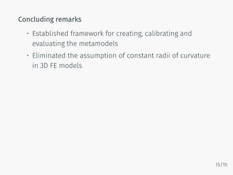
Concluding remarks

• Established framework for creating, calibrating andevaluating the metamodels

• Eliminated the assumption of constant radii of curvaturein 3D FE models

• Assessed the accuracy of the current metamodel

Outlook

• Improve the accuracy of the metamodel• Extend it to handle cases involving non-linear materialresponse

15/15

Concluding remarks

• Established framework for creating, calibrating andevaluating the metamodels

• Eliminated the assumption of constant radii of curvaturein 3D FE models

• Assessed the accuracy of the current metamodel

Outlook

• Improve the accuracy of the metamodel

• Extend it to handle cases involving non-linear materialresponse

15/15

Concluding remarks

• Established framework for creating, calibrating andevaluating the metamodels

• Eliminated the assumption of constant radii of curvaturein 3D FE models

• Assessed the accuracy of the current metamodel

Outlook

• Improve the accuracy of the metamodel• Extend it to handle cases involving non-linear materialresponse

15/15

Thank you for attention!

Johansson, A., Pålsson, B., Ekh, M., Nielsen, J. C. O., Ander, M.K. A., Brouzoulis, J., and Kassa, E. (2011).Simulation of wheel-rail contact and damage in switches& crossings.Wear, 271(1-2):472–481.

Shepard, D. (1968).A two-dimensional interpolation function forirregularly-spaced data.In Proceedings of the 1968 23rd ACM national conference,pages 517–524. ACM.