ON MODELING OF GEOPHYSICAL PROBLEMS

A Dissertation

Presented to the Faculty of the Graduate School

of Cornell University

in Partial Fulfillment of the Requirements for the Degree of

Doctor of Philosophy

by

Robert Shcherbakov

August 2002

c© Robert Shcherbakov 2002

ALL RIGHTS RESERVED

ON MODELING OF GEOPHYSICAL PROBLEMS

Robert Shcherbakov, Ph.D.

Cornell University 2002

This dissertation models some aspects of the physics of earthquakes and obtains

estimates of the thickness and density of the Martian crust and elastic lithosphere.

Specifically, we treat earthquakes utilizing the dynamics of a highly nonlinear sys-

tem which we associate with the upper brittle layer of the Earth. We consider

two models of self-organized criticality (SOC) (height-arrow model and Eulerian

walker model) which exhibit a scaling behavior similar to the Gutenberg-Richter

frequency-magnitude law for earthquakes. The models are studied by numerical

simulations and analytical methods. Another aspect of earthquake physics, the ir-

reversible processes which produce seismic events and cause deformations of the

crust, is considered from the damage mechanics point of view. The solutions of

the fiber-bundle model and several models of continuum damage mechanics allow

us to quantify the seismic activation prior to large earthquakes (increases in Benioff

strain) and to study relaxation processes (aftershocks) following large events.

We further report on the study of the thickness and density of the Martian crust

and elastic lithosphere. Using recent data, obtained from the Mars Global Surveyor

mission, we are able to constrain the thicknesses of both the Martian crust and

elastic lithosphere to 90± 10 km. To accomplish this we use the assumption of Airy

type compensation for the Hellas basin and wavelet transform analyses of the global

circle tracks of gravity and topography. We also find that the mean crustal density

is 2, 960± 50 kg m−3.

Biographical Sketch

Robert Shcherbakov was born on April 19, 1970, in Dilidjan, Armenia, USSR. When

he was six his family moved back to Yerevan where he attended Yerevan school #132

and in 1987 matriculated at Yerevan State University, Physics Department, which

he successfully graduated in June of 1992. In December 1993 he moved to Russia.

After spending four and a half years at Joint Institute for Nuclear Research in

Dubna, Russia, Robert began graduate studies at Cornell University in the Fall of

1998.

iii

To my awesome mother, Irina, for her love and encouragement

iv

Acknowledgements

First of all, I would like to thank my advisor Donald Turcotte for his enthusiastic

and encouraging support and advice for my last four years at Cornell. It has been

a great pleasure to work with him. His combination of wide-ranging knowledge and

intuitive understanding of natural phenomena have made him an inspiring person

to work with.

My special thanks go to Larry Brown and Bart Selman for serving on my special

committee and for their useful comments and advice.

A very grateful thanks are due to my former advisors, Nerses Ananikian and

Vyacheslav Priezzhev, who introduced me to the world of theoretical physics and

the scientific way of thinking.

Special thanks also go to my collaborators with whom I’ve had the opportunity

to work in the last decade or so: Ruben Ghulghazaryan, Nikolai Izmailyan, Algis

Kucinskas, Bruce Malamud, William Newman, Vladimir Papoyan Jr., and Alexan-

der Povolotsky. I also would like to thank Deepak Dhar, Eugene Ivashkevich, Dimitri

Ktitarev, Gleb Morein, Vladimir Papoyan, Bosiljka Tadic, Valery Ter-Antonyan, for

many valuable and stimulating discussions.

Many special thanks to all my friends with whom I’ve had the chance to spent

so many interesting and exciting moments discussing music, physics and philosophy,

v

playing games, and just doing nothing: Anatoli Astvatsatourov, Georgios Athanas-

siadis, Andrei Baliakin, Hrant Dadivanyan, Julia Epifantseva, Tatiana Filipova,

Yeranuhi Hakobyan, Nigiar Hashimzade, Armen Laziev, Khajak Karayan, Sergey

Kiselev, Alexei Kisselev, Olga Korneichuk, Daria Kriminskaia, Sergey Kriminski, Ar-

men Laziev, Daniel Levin, Brola Lordkipanidze, Nona Mahari, Armen Manukyan,

Tigran Martirosyan, Sergey Mesropian, Vasile Nistor, Anatoli Olkhovets, Natalia

Perkins, Mikhail Polianski, Dmitri Ponarin, Ludmila Rovba, Vera Sazonova, Valerii

Smirichinski, Irene Shifman, Darina Stankeyeva, Simon Ter-Antonyan, Maxim Vav-

ilov, Lilit Yeghiazarian, Emil Yuzbashyan, and many others whom I’ve forgotten to

mention here.

vi

Table of Contents

1 Introduction 11.1 Earthquakes . . . . . . . . . . . . . . . . . . . . . . . . . . . . . . . . 1

1.1.1 Physics of earthquakes . . . . . . . . . . . . . . . . . . . . . . 31.1.2 Self-organized criticality . . . . . . . . . . . . . . . . . . . . . 141.1.3 Fracture of solids and statistical physics . . . . . . . . . . . . 22

1.2 Martian figure and internal composition . . . . . . . . . . . . . . . . 321.2.1 Topography, gravity field, and planetary interior . . . . . . . . 321.2.2 Hydrostatic considerations . . . . . . . . . . . . . . . . . . . . 34

1.3 Outline . . . . . . . . . . . . . . . . . . . . . . . . . . . . . . . . . . . 37

2 Models of self-organized criticality 382.1 Self-organizing height-arrow model . . . . . . . . . . . . . . . . . . . 41

2.1.1 The model on the square lattice. . . . . . . . . . . . . . . . . . 412.1.2 Numerical results. . . . . . . . . . . . . . . . . . . . . . . . . . 432.1.3 The height-arrow model on the Bethe lattice. . . . . . . . . . 562.1.4 The avalanche structure on the Bethe lattice. . . . . . . . . . 62

2.2 Eulerian walkers model . . . . . . . . . . . . . . . . . . . . . . . . . . 652.2.1 Algebraic properties of the model . . . . . . . . . . . . . . . . 652.2.2 Avalanche dynamics . . . . . . . . . . . . . . . . . . . . . . . 702.2.3 Numerical simulations . . . . . . . . . . . . . . . . . . . . . . 772.2.4 Diffusion of Eulerian walkers . . . . . . . . . . . . . . . . . . . 83

3 Earthquakes and Damage Mechanics 893.1 Micro- and macro-scopic models of fracture and damage . . . . . . . 89

3.1.1 Introduction . . . . . . . . . . . . . . . . . . . . . . . . . . . . 893.1.2 Fiber-bundle model . . . . . . . . . . . . . . . . . . . . . . . . 933.1.3 Damage model . . . . . . . . . . . . . . . . . . . . . . . . . . 993.1.4 Generalized damage model . . . . . . . . . . . . . . . . . . . . 1013.1.5 Time dependent stress . . . . . . . . . . . . . . . . . . . . . . 1033.1.6 Acoustic emission events . . . . . . . . . . . . . . . . . . . . . 1083.1.7 Seismic activation . . . . . . . . . . . . . . . . . . . . . . . . . 1143.1.8 Discussion . . . . . . . . . . . . . . . . . . . . . . . . . . . . . 114

3.2 Aftershocks and stress relaxation . . . . . . . . . . . . . . . . . . . . 116

vii

3.2.1 Constant applied strain . . . . . . . . . . . . . . . . . . . . . . 1173.2.2 Stress increasing linearly with time . . . . . . . . . . . . . . . 1213.2.3 Strain increasing linearly with time . . . . . . . . . . . . . . . 1263.2.4 Discussion . . . . . . . . . . . . . . . . . . . . . . . . . . . . . 130

4 Martian crust and Martian elastic lithosphere 1324.1 Global Data . . . . . . . . . . . . . . . . . . . . . . . . . . . . . . . . 1324.2 Hellas Analysis . . . . . . . . . . . . . . . . . . . . . . . . . . . . . . 1434.3 Compensation . . . . . . . . . . . . . . . . . . . . . . . . . . . . . . . 1494.4 Wavelet Analysis . . . . . . . . . . . . . . . . . . . . . . . . . . . . . 1554.5 Discussion . . . . . . . . . . . . . . . . . . . . . . . . . . . . . . . . . 165

5 Conclusion 169

A Finite-size scaling analysis 175A.1 Simple scaling . . . . . . . . . . . . . . . . . . . . . . . . . . . . . . . 175

B Wavelet analysis 178B.1 One dimensional wavelet transform . . . . . . . . . . . . . . . . . . . 178

Bibliography 180

viii

List of Tables

2.1 The time average density pc of occupied sites for the HA model . . . 542.2 The critical exponents for the 2d HA model . . . . . . . . . . . . . . 55

4.1 Mars parameter values used and derived . . . . . . . . . . . . . . . . 137

ix

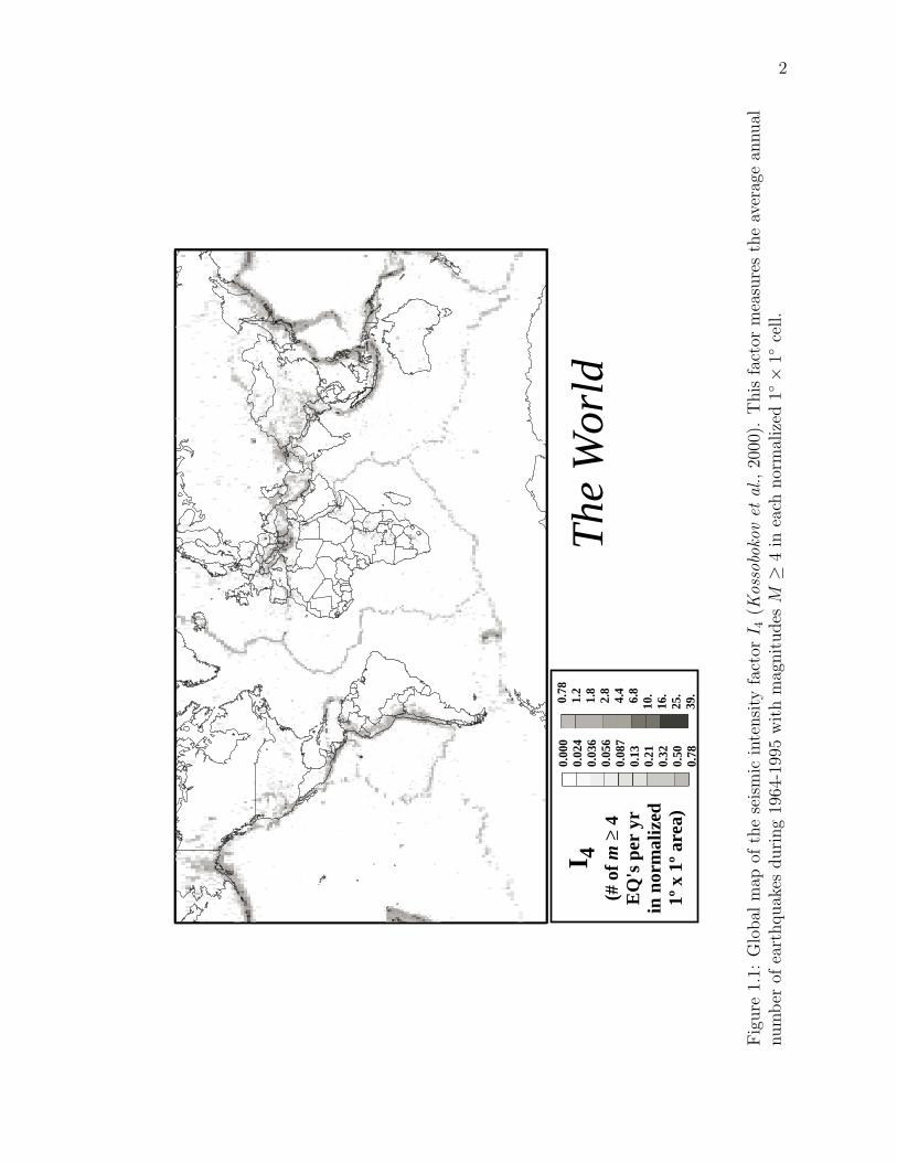
List of Figures

1.1 Global map of the seismic intensity factor I4 . . . . . . . . . . . . . . 21.2 The Gutenberg-Richter relation for southern California . . . . . . . . 71.3 Power-law increase in the cumulative Benioff strain . . . . . . . . . . 101.4 Illustration of the two dimensional spring-block model. . . . . . . . . 191.5 Schematic pressure-volume diagram of a pure substance . . . . . . . 261.6 Idealized stress-strain diagram for a brittle solid . . . . . . . . . . . . 29

2.1 A computer simulation of the HA model . . . . . . . . . . . . . . . . 442.2 The dependence of the time average density of occupied sites . . . . 452.3 A typical form of an avalanche cluster of the HA model . . . . . . . 472.4 Double-logarithmic plot of the binned distributions of avalanches . . 482.4 continued . . . . . . . . . . . . . . . . . . . . . . . . . . . . . . . . . 492.5 Double-logarithmic plot of the dependence of the stochastic variables 502.5 continued . . . . . . . . . . . . . . . . . . . . . . . . . . . . . . . . . 512.6 Double-logarithmic plot of the finite-size scaling . . . . . . . . . . . . 522.7 Double-logarithmic plot of the finite-size scaling . . . . . . . . . . . . 532.8 Construction of the Cayley tree . . . . . . . . . . . . . . . . . . . . . 562.9 A kth-generation branch Tk and vertex b form a subgraph T ′ . . . . 582.10 Two examples of strongly and weakly allowed configurations . . . . . 592.11 A kth-generation branch Tk consists of three nearest branches . . . . 592.12 A site O with height zo = n and a given direction of the arrow . . . . 622.13 Three possible configurations of avalanche clusters of size s = 2 . . . 632.14 The structure of avalanche evolution in EW model . . . . . . . . . . 722.15 The distribution of duration of the first avalanche . . . . . . . . . . . 752.16 Distribution P (s) of the number of visited sites in avalanches . . . . 782.17 The integrated distributions D(s) for the eight lattice sizes . . . . . . 802.18 The finite-size scaling for the integrated distributions D(s) . . . . . . 812.19 The distribution P (l) of the number of steps in avalanches . . . . . . 822.20 A subsequent evolution of a cluster of visited sites in the SOC state . 842.21 The dependence of the mean square displacement of the particle . . . 87

3.1 Schematic illustration of the failure of a brittle rod . . . . . . . . . . 913.2 Schematic illustration of the failure of a fiber-bundle . . . . . . . . . 943.3 Dependence of the ratio of the effective Young’s modulus . . . . . . . 98

x

3.4 Dependence of the ratio of the effective Young’s modulus . . . . . . . 1063.5 Cumulative acoustic energy emissions . . . . . . . . . . . . . . . . . 1133.6 Stress relaxation after the instantaneous application of a strain . . . 1193.7 Dependence of the damage variable α . . . . . . . . . . . . . . . . . 1233.8 Dependence of the nondimensional failure time tf/ty . . . . . . . . . 1243.9 Illustration of the power-law scaling . . . . . . . . . . . . . . . . . . 1253.10 Dependence of the nondimensional stress on strain . . . . . . . . . . 1273.11 Dependence of the damage variable α on time . . . . . . . . . . . . . 1283.12 Dependence of the nondimensional stress on strain . . . . . . . . . . 129

4.1 The figure of Mars is given on two great circle tracks. . . . . . . . . . 1344.2 The areoid of Mars is given on two great circle tracks. . . . . . . . . 1404.3 The topography of Mars is given on two great-circle tracks . . . . . . 1444.4 Topography and areoid across Hellas basin . . . . . . . . . . . . . . . 1464.5 Dependence of the areoid anomalies on the topography . . . . . . . . 1474.6 Power spectral density coefficients of the Martian figure . . . . . . . 1534.7 Power spectral density coefficients of the Martian areoid . . . . . . . 1544.8 Dependence of the ratio of gravity on topography . . . . . . . . . . . 1564.9 Wavelet analysis of MOLA topography . . . . . . . . . . . . . . . . . 1584.10 Wavelet variance analysis of Martian topography . . . . . . . . . . . 1594.11 Wavelet analysis of MGS gravity data . . . . . . . . . . . . . . . . . 1614.12 Wavelet variance analysis of Martian gravity data . . . . . . . . . . . 1624.13 The gravity-topography admittances . . . . . . . . . . . . . . . . . . 163

xi

Chapter 1

Introduction

1.1 Earthquakes

Studies of earthquake physics are one of the most interesting and challenging prob-

lems in modern geophysics. Progress in understanding the dynamics, mechanical

properties, chemistry, and other aspects of earthquakes is crucial for both the sci-

entific community and society at large. As a consequence, a better understanding

of earthquakes will facilitate the development of different prediction techniques that

are of tremendous significance for many aspects of our life.

It has turned out that historically people tend to live in the most active, seis-

mogenic zones. One explanation for this phenomenon is the location of these zones

near sea shores where in many cases subduction or collision of oceanic plates and

continental ones occur and as a consequence earthquakes and volcanic eruptions

take place. Such zones are easily identified on the global map of seismogenic activ-

ity on the Earth (Figure 1.1). Examples are California, Japan, Greece, Italy, Chile,

New Zealand and other areas. Therefore, the hazard risk assessment of these re-

gions strongly depends on our current state of knowledge about the processes which

1

2

The

Wor

ldI 4

(# o

f m

≥ 4

EQ

's p

er y

rin

nor

mal

ized

1º x

1º

area

)

0.78

1.2

1.8

2.8

4.4

6.8

10.

16.

25.

39.

0.00

00.

024

0.03

60.

056

0.08

70.

130.

210.

320.

500.

78

Fig

ure

1.1:

Glo

bal

map

ofth

ese

ism

icin

tensi

tyfa

ctorI 4

(Kos

sobo

kov

etal

.,20

00).

This

fact

orm

easu

res

the

aver

age

annual

num

ber

ofea

rthquak

esduri

ng

1964

-199

5w

ith

mag

nit

udesM≥

4in

each

nor

mal

ized

1×

1ce

ll.

3

control earthquake occurrence.

In the most recent fifty years or so a great deal of effort has been devoted to

trying to develop a comprehensive theory of earthquakes and to devise techniques for

their prediction. Unfortunately, in many cases these methods or precursors are not

reliable or work only in retrospective studies. This has created some scepticism in the

geophysical community about the predictability of such events. Several researches

went even further by declaring that earthquakes are not predictable at all (Geller et

al., 1997). Nevertheless, we believe that we do not possess enough information and

knowledge to answer this question at this point. Further research and new ideas are

crucial in the quest to understand and predict earthquakes.

1.1.1 Physics of earthquakes

Earthquakes represent a very complicated outcome of the processes which take place

in the brittle outer layer of the earth, or schizosphere (Sornette, 1999; Scholz, 2002).

From the physics point of view, this layer can be considered as a highly nonlinear dis-

sipative dynamic system which exhibits extremely complicated behavior (Sornette,

2000). To understand this behavior and as a consequence to be able to predict

earthquakes one has to exploit all available knowledge in the theories of nonlinear

dynamics, rupture theory, damage mechanics, nonequilibrium statistical mechanics,

stochastic processes, chemistry, fluid dynamics, and many other areas of modern

science.

Studies of earthquakes reveal that most shallow earthquakes occur in zones of

collision of continental and oceanic plates. Mid-oceanic ridges, where the creation

of new oceanic plates take place, are other zones of occurrence of shallow earth-

quakes. Another group consists of earthquakes which occur at greater depths and

4

are associated with mechanical and thermal processes in the descending oceanic

slabs subjected to high stresses and temperatures. The interior of continental plates

are also prone to earthquakes although with much lower rates of occurrence. The

famous example is the New Madrid area in Missouri, USA. And finally, there are so

called induced earthquakes which are the result of different human activities such

as the construction of dams, mining, and nuclear explosions.

A. Dynamic faulting

It is now accepted that the origin of the majority of earthquakes is dynamic fault-

ing. The accumulation of the strain in the crust due to tectonic processes leads to

instability which occurs suddenly and a rupture dynamically propagates along the

fault. This slip generates seismic waves and is the mechanism for most common and

important type of earthquakes.

From the dynamic faulting point of view an earthquake may be treated as a

dynamically running shear crack. For this process it is worth while to write down

the energy balance (Kostrov and Das, 1988)

∆Ep = Es + Ef + Ed , (1.1.1)

where ∆Ep is the potential energy change due to changes in elastic and gravitational

energies during an earthquake, Es is the seismic energy during an earthquake, Ef is

the work done by frictional forces on the fault, and Ed is the damage energy involved

in the creation of cracks.

Radiated seismic energy Es is defined as the total energy transmitted by seismic

waves through a surface S0 surrounding the source. With several approximation it

is possible to show that the radiated seismic energy has the form (Kostrov and Das,

5

1988; Scholz, 2002)

Es ≈1

2∆σ∆uA , (1.1.2)

where ∆σ is a static shear stress drop, ∆u is a mean slip, and A is a fault area.

In modeling of earthquakes as dynamic rupture processes there are two ap-

proaches describing the mechanism of rupture as unstable slip. One treats it as

a brittle fracture and assumes that a characteristic fracture energy per unit area, a

material property, is required for the crack to propagate. In the second approach,

rupture is assumed to occur when the stress on the fault reaches the static friction

threshold. This leads to so-called stick-slip behavior. These two approaches are

mathematically equivalent but have traditionally differed in the way in which the

rupture process is considered.

Another problem arises when one tries to apply solutions of some idealized mod-

els to the real cases. Ruptures in rock and the Earth’s crust are subjected to

more complicated conditions. They are described by complex geometry, and the

parameters which govern the dynamics are likely to be heterogeneous at all scales.

Therefore, simplified models do not reflect all the complexities of the dynamics of

real processes and as a result cannot be applied directly. On the other hand, they

help to understand the physics underlying the mechanism of earthquakes.

B. Gutenberg-Richter scaling

The observation and documentation of earthquakes are mostly done by recording the

precise date and time, depth, magnitude and some other parameters of earthquakes.

This data is organized in catalogs and in most cases is available for study.

The magnitude is a traditional measure of earthquake size and is based on the

logarithm of the amplitude of a specified seismic wave measured at a particular

6

frequency, suitably corrected for distance and instrument response (Scholz, 2002).

Therefore, one can calculate several types of magnitudes (mL, mb, Ms, Mw) for a

given earthquake based on the measured wave type.

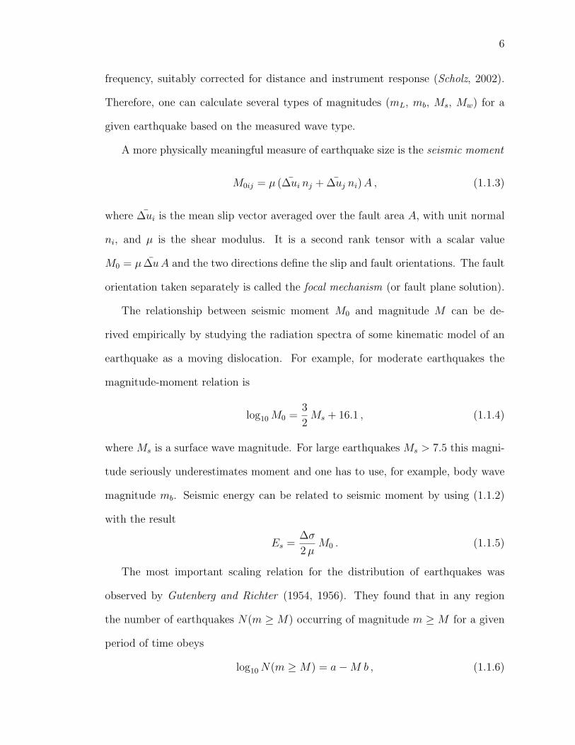
A more physically meaningful measure of earthquake size is the seismic moment

M0ij = µ (∆ui nj + ∆uj ni)A , (1.1.3)

where ∆ui is the mean slip vector averaged over the fault area A, with unit normal

ni, and µ is the shear modulus. It is a second rank tensor with a scalar value

M0 = µ ∆uA and the two directions define the slip and fault orientations. The fault

orientation taken separately is called the focal mechanism (or fault plane solution).

The relationship between seismic moment M0 and magnitude M can be de-

rived empirically by studying the radiation spectra of some kinematic model of an

earthquake as a moving dislocation. For example, for moderate earthquakes the

magnitude-moment relation is

log10M0 =3

2Ms + 16.1 , (1.1.4)

where Ms is a surface wave magnitude. For large earthquakes Ms > 7.5 this magni-

tude seriously underestimates moment and one has to use, for example, body wave

magnitude mb. Seismic energy can be related to seismic moment by using (1.1.2)

with the result

Es =∆σ

2µM0 . (1.1.5)

The most important scaling relation for the distribution of earthquakes was

observed by Gutenberg and Richter (1954, 1956). They found that in any region

the number of earthquakes N(m ≥ M) occurring of magnitude m ≥ M for a given

period of time obeys

log10N(m ≥M) = a−M b , (1.1.6)

7

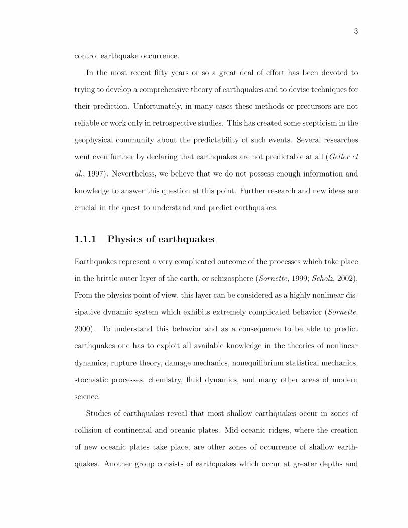
0 1 2 3 4 5 6 7 8

0

1

2

3

4

5

6

Log 10

(N(>

M))

M

Data (20N-40N)x(125W-100W) Fit (slope = -0.95)

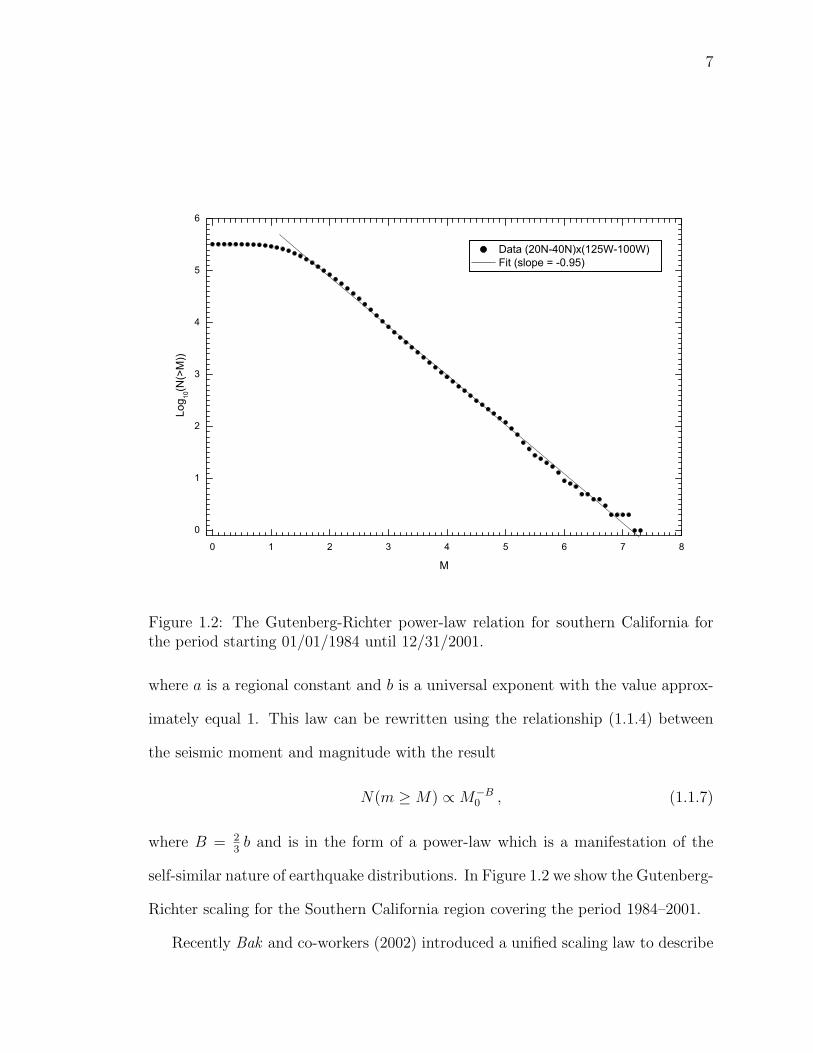
Figure 1.2: The Gutenberg-Richter power-law relation for southern California forthe period starting 01/01/1984 until 12/31/2001.

where a is a regional constant and b is a universal exponent with the value approx-

imately equal 1. This law can be rewritten using the relationship (1.1.4) between

the seismic moment and magnitude with the result

N(m ≥M) ∝M−B0 , (1.1.7)

where B = 23b and is in the form of a power-law which is a manifestation of the

self-similar nature of earthquake distributions. In Figure 1.2 we show the Gutenberg-

Richter scaling for the Southern California region covering the period 1984–2001.

Recently Bak and co-workers (2002) introduced a unified scaling law to describe

8

the waiting times between earthquakes. From their analysis it follows that there is no

unique way of distinguishing between foreshocks, mainshocks, and aftershocks. The

Gutenberg-Richter b value, the exponent p of the modified Omori’s law (see below)

for aftershocks, and the fractal dimension df of the distribution of earthquakes

epicenters appear as critical indices in the their unified law for earthquakes.

C. Earthquake sequences and clustering

Another important aspect of earthquakes is their tendency to form clusters in space

and time. Space clustering sometimes but not always is possible to explain by the

geometry of faults. Whereas time clustering is the result of the complex dynamics of

stress redistribution and interactions among faults following previous earthquakes.

It has been recognized that after a large earthquake one can observe a significant

increase in earthquake activity in the vicinity of this large earthquake. These smaller

earthquakes constitute aftershocks of the mainshock. A mainshock in many cases is

preceded by a sequence of earthquakes which are called foreshocks. The sequence of

earthquakes without a pronounced mainshock has been called a swarm. Two or more

mainshocks occurring closely in space and time constitute compound earthquakes.

These definitions of sequences are rather descriptive and not always precise.

The problem arises when an aftershock creates its own sequence of aftershocks or

a mainshock that might be an aftershock of one of its foreshocks. These types

of observations lead to two different approaches to the classification of earthquakes.

One approach classifies differences between foreshocks, mainshocks, aftershocks, and

isolated events on the basis of different mechanisms that are responsible for each

sequence. The other approach states that the mechanisms of all earthquakes are the

same. Moreover, all earthquakes are capable of producing aftershocks, and in turn

aftershocks produce their own aftershock sequences (Helmstetter and Sornette, 2002;

9

Sornette and Helmstetter, 2002). In addition, earthquakes can trigger aftershocks

larger than themselves and aftershocks appear identical to other earthquakes. For

example, there is strong observational evidence that the 1999 magnitude 7.1 Hector

Mine earthquake in the Mojave Desert, California, was triggered by a chain of

aftershocks that was initiated by the 1992 magnitude 7.3 Landers earthquake (Felzer

et al., 2002).

Despite these difficulties, there are several empirical relationships describing the

behavior of earthquake sequences. One of them is a modified Omori’s law which

describes the decay of aftershock activity (Utsu, 1961)

dNas

dt=

C1

[C2 − (t− tms)]p, (1.1.8)

where Nas is the number of aftershocks at time t, t − tms is time elapsed after

the mainshock. C1 is a rate constant and C2 is a constant with units of time and

regularizes the singularity at t = tms. The exponent p has a universal value near 1.

Several authors have previously given explanations for Omori’s law. One ap-

proach utilizes viscoelastic relaxation in the crust (Nakanishi, 1992). But this ap-

proach does not explain the universal occurrence of aftershocks. Das and Scholz

(1981) utilized stress corrosion combined with a critical stress intensity factor. Shaw

(1993) utilized a phenomenological approach to the dynamics of subcritical crack

growth. Dietrich (1994) has related the power-law decrease in aftershock activity to

the rate and state friction law. Rundle et al. (1999) associate aftershock sequences

with the power-law scaling in the vicinity of a spinodal.

Another empirical relationship, also known as Bath’s law, states that the average

difference in size between a mainshock and its largest aftershock is 1.2 magnitude

units, regardless of the mainshock magnitude (Richter, 1958; Bath, 1965).

Systematic increases in the intermediate level of seismicity prior to large earth-

10

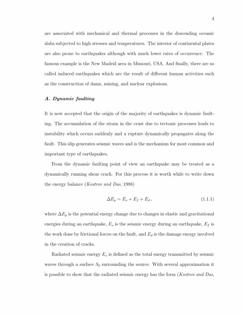
1910 1920 1930 1940 1950 19600

5

20

10

15

Cum

ulat

ive

Ben

ioff

Str

ain

(x10

7 )

Kern County

Date

Date

0

2

10

Cum

ulat

ive

Ben

ioff

Str

ain

(x10

7 )

Loma Prieta

4

6

8

1910 1920 1930 1940 1950 1960 1970 1980 19900.0

0.5

2.0

1.0

1.5

Cum

ulat

ive

Ben

ioff

Str

ain

(x10

7 )Coalinga

Date1980 1980 1981 1981 1982 1982 1983 1983

Date

0

2

10

Cum

ulat

ive

Ben

ioff

Str

ain

(x10

7 )

Landers

4

6

8

1970 1975 1980 1985 1990 1995

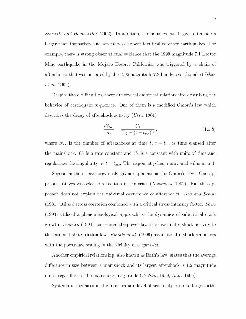
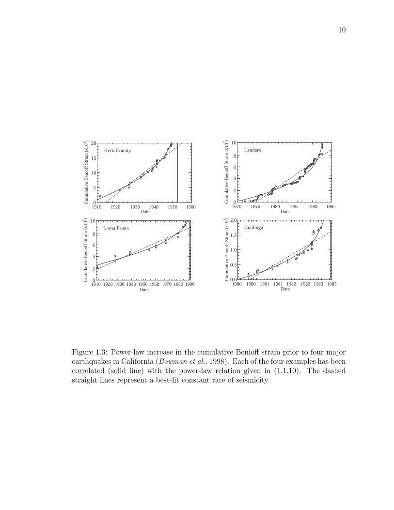
Figure 1.3: Power-law increase in the cumulative Benioff strain prior to four majorearthquakes in California (Bowman et al., 1998). Each of the four examples has beencorrelated (solid line) with the power-law relation given in (1.1.10). The dashedstraight lines represent a best-fit constant rate of seismicity.

11

quakes have been proposed by several authors (Sykes and Jaume, 1990; Knopoff et

al., 1996; Jaume and Sykes, 1999). It has also been observed that there is a power-

law increase in seismic activity prior to major earthquake. This was first proposed

by Bufe and Varnes (1993). They considered the cumulative Benioff strain in a

region defined as

εB(t) =N(t)∑i=1

√Ei , (1.1.9)

where Ei is the seismic energy release in the ith precursory earthquake and N(t)

is the number of precursory earthquakes considered up to time t. Bowman et al.

(1998) carried out a systematic study of the optimal spatial region and magnitude

range to obtain power-law activation. Four examples of their results are given in

Figure 1.3. In each case εB(t) has been correlated with the relation

εB(t) = εBf −B

(1− t

tf

)s

, (1.1.10)

where εBf is the cumulative Benioff strain when the large earthquake occurs, tf is the

time since the last large earthquake, and B is a constant. For the four earthquakes

illustrated in Figure 1.3 it is found that s = 0.30 (Kern County), s = 0.18 (Landers),

s = 0.28 (Loma Prieta), and s = 0.18 (Coalinga). Other examples of power-law

seismic activation have been given by Buffe et al. (1994); Varnes and Bufe (1996);

Brehm and Braile (1998, 1999); Robinson (2000); and Zoller et al. (2001).

D. Friction

Friction plays a crucial role in earthquake dynamics. It was probably Brace and

Byerlee (1966) who first suggested friction to be a mechanism for earthquakes. Al-

though big advances were made during the last years in understanding frictional

processes, we still lack a comprehensive theory of friction and its role in earthquake

physics.

12

The history of frictional studies goes back to Leonardo da Vinci, who discovered

two basic laws of friction. They were rediscovered by Amonton de la Hire in 1699

and state (Scholz, 2002):

i) The frictional force per unit area is independent of the size of the surface in

contact.

ii) Friction is proportional to the normal load.

The second law can be expressed mathematically as

F = µN , (1.1.11)

where F is the friction force, N is the normal load, and µ is a coefficient of friction.

Later, Coulomb recognized the difference between static friction (µs) and dy-

namic friction (µd). It was observed that the former is higher than the later

µ =

µs if v = 0

µd if v > 0, (1.1.12)

where v is the velocity between sliding surfaces.

Modern theories of friction went further and now include the dependence of the

coefficient of friction µ on velocity, slip, time, etc. The friction law (1.1.11) itself is

only valid to the first approximation. The effects of lubrication, roughness, hardness,

temperature and ductility, pore fluids, wear due to damage require more complicated

laws including a nonlinear dependence of the frictional force on normal loading. One

approach to friction is to consider different theoretical models on a mesoscopic level

and try to reproduce the macroscopic phenomena. From many experimental results

the frictional force between two sliding surfaces can be viewed as a macroscopic

average of the resistance to motion due to various microscopic interactions among

13

asperities on these surfaces. The nature of these interactions could have different

sources. Other important aspects of friction are energy dissipation and frictional

wear due to damage. It is also important to recognize that friction is a result of

different processes that occur simultaneously in a very complex way.

The difference between static and dynamic friction naturally leads to dynamic

instabilities in the system. Consider, for example, a massive block loaded through a

spring with stiffness k sliding on some surface. When the force F = k x, where x is

a displacement, acting on the block through the spring exceeds the critical value of

the static frictional resistive force Fs = µsN , where N is a normal force, the block

starts to move. At the beginning, the block accelerates as the dynamic resistive

frictional force Fd = µdN is less than pulling force F . However, at some point Fd

becomes greater than F and the block comes to the rest and the stress starts to

build up again. This type of repetitive behavior is called stick-slip.

The understanding of mechanisms of static and dynamic friction was advanced

by several authors (Rabinowicz, 1965; Dieterich, 1978, 1979; Ruina, 1983). The first

observation was that the static coefficient of friction µs increases with the waiting

time ts prior to sliding. This is described by a logarithmic law:

µs(ts) = µs0 + A ln(tsL

), (1.1.13)

where µs0 is some base friction, L is a characteristic sliding distance, and A is a

constant. This law describes the “aging” of the static friction (Scholz, 2002).

The second observation concerns dynamic friction. Laboratory studies of fric-

tional instabilities have led to the general acceptance of an empirical rate- and

state-dependent friction law (Dieterich, 1979; Ruina, 1983). A widely used form of

14

this law is given by

µd = µd0 + a ln(v

v0

)+ b ln

(v0 θ

Dc

), (1.1.14)

dθ

dt= 1− v0 θ

Dc

, (1.1.15)

where µd is the coefficient of friction at slip velocity v, µd0 is the coefficient of

friction at slip velocity v0, θ is a “state” variable, and a, b, and Dc are constants.

When the slip velocity v changes instantaneously, the state variable relaxes to a new

equilibrium value.

1.1.2 Self-organized criticality

In 1987 Bak and his co-workers (1987, 1988, 1989, 1996) proposed a concept of self-

organized criticality (SOC), a holistic theory intended to describe the behavior of

large externally driven dissipative dynamic systems consisting of many interacting

elements (for the reviews on SOC see Bak (1996); Jensen (1998); Vespignani and

Zapperi 1998; Turcotte (1999a)). Their research was motivated by the ubiquitous

presence of scale invariant temporal and spatial structures (fractals) (Mandelbrot,

1982) and 1/f noise (Feder, 1989) in nature and particularly the Gutenberg-Richter

distribution of the number of earthquakes versus magnitude (Gutenberg and Richter,

1954).

The essential characteristics of a system that evolves into the SOC state and

stays there are

i) Dissipation: The system interacts with the outer world through external driv-

ing and releases energy by instabilities (avalanches) in the process of evolution.

ii) Slow external driving : The pumping of energy into the system organizes it

15

into the stationary state and compensates for the loss of energy due to the

dissipative nature of the system.

iii) Separation of time scales : Slow driving rate and fast release of energy through

avalanche dynamics are necessary conditions for the system to get into the

SOC state. This separation of time scales can be considered as a control

parameter of the system (Vespignani and Zapperi, 1997, 1998).

iv) Threshold dynamics : It is one of the crucial aspects of the evolution of the sys-

tem and defines the process of relaxation of the local field when it exceeds some

critical value. These relaxations lead to cascade type behavior and avalanches

emerge in the system.

v) Scale-invariant avalanche statistics : The frequency-size distributions of event

sizes (avalanches) must follow a power-law behavior which signifies long-range

spatial and temporal correlations in the SOC state.

Despite a great deal of research activity in experiments, theory, and computer

modeling and as a consequence a tremendous number of articles published after the

introduction of the SOC theory, the current understanding of physical mechanisms

which govern the behavior of the highly-nonlinear dissipative dynamic systems is still

illusive. It’s turned out that SOC in it’s original form is too simplistic to describe

such systems (Sornette and Helmstetter, 2002).

Recent research suggests that many systems show fluctuations around the SOC

state, i.e., system dynamics builds long-range correlations in the system and pro-

duces power-law distributions of event sizes before a large avalanche destroys this

correlated state. The system retreats from the SOC state only to start its process

of rebuilding of long-range correlations. This idea is appealing from the geophysical

16

point of view and could explain the existence of characteristic earthquakes.

In this context it is interesting to mention the work by Wolfram (2002) where he

suggests that the cellular automaton approach is A New Kind of Science in study-

ing complexity and physical phenomena at large. Dynamics generated by cellular

automata of different types show four separate patterns: dull uniformity, periodic

time-dependence, fractal behavior, and truly complex nonrepetitive patterns. Using

these concepts he discusses fractals, the idea of universal computation, the genera-

tion of complex patterns, quantum physics, gravity, etc.

A. Sandpile models

The original Abelian sandpile model (ASM) was introduced by Bak and co-workers

as a paradigm of self-organized criticality (Bak et al., 1987, 1988). The model can

be formulated on any connected graph and possesses very rich nontrivial behav-

iors. The definitions of the SOC state of the model through recursive and transient

configurations and the calculation of the distribution of heights were obtained by

the groups of Dhar and Priezzhev (Dhar, 1990, 1999; Majumdar and Dhar, 1991,

1992; Priezzhev, 1994; Ivashkevich and Priezzhev, 1998). The structure of avalanche

processes and the exact calculation of the critical exponents were done by Priez-

zhev et al. 1996a. The model was also considered on tree like Bethe lattice (Dhar

and Majumdar, 1990), Husimi lattices (Papoyan and Shcherbakov, 1995, 1996), and

fractal type lattices (Kutnjak-Urbanc et al., 1996; Daerden et al., 1998, 2001). A

real space renormalization group method was devised to obtain good estimates of

the avalanche exponents (Vespignani et al., 1995; Ivashkevich, 1996; Ivashkevich et

al., 1999). More recently, the large scale simulations revealed a more complicated

multiscaling structure of avalanches in the ASM (De Menech etal., 1998; Tebaldi et

al., 1999; De Menech and Stella, 2000; Ktitarev et al., 2000).

17

The “avalanche” of papers published in the last two decades were also devoted to

the study of many modifications and variations of the original ASM. Among them

it is interesting to note the different stochastic versions. Manna (1991) studied the

two-state model and found different critical exponents which was the reflection of a

non-compact structure of avalanches and stochasticity of the dynamics. The directed

stochastic sandpiles were also studied by several authors (Tadic, 1999; Kloster et

al., 2001).

These advances in studying different models naturally raised the question of

classes of universality for these models. There were several attempts to shed light on

this problem (Milstein et al., 1998; Chessa et al., 1999; Biham et al., 2001). However,

the final answer to the question whether these models belong to several distinct

universality classes or there is a continuum of universality classes still remains open.

B. Spring-block models

The spring-block model was introduced by Burrige and Knopoff (1967) to model

the behavior of a single fault. The model reproduces the Gutenberg-Richter scaling

law (1.1.7) and is a basis for many numerical models of real faults. The original

version of the model was one dimensional. Several modifications of the model were

studied by different authors.

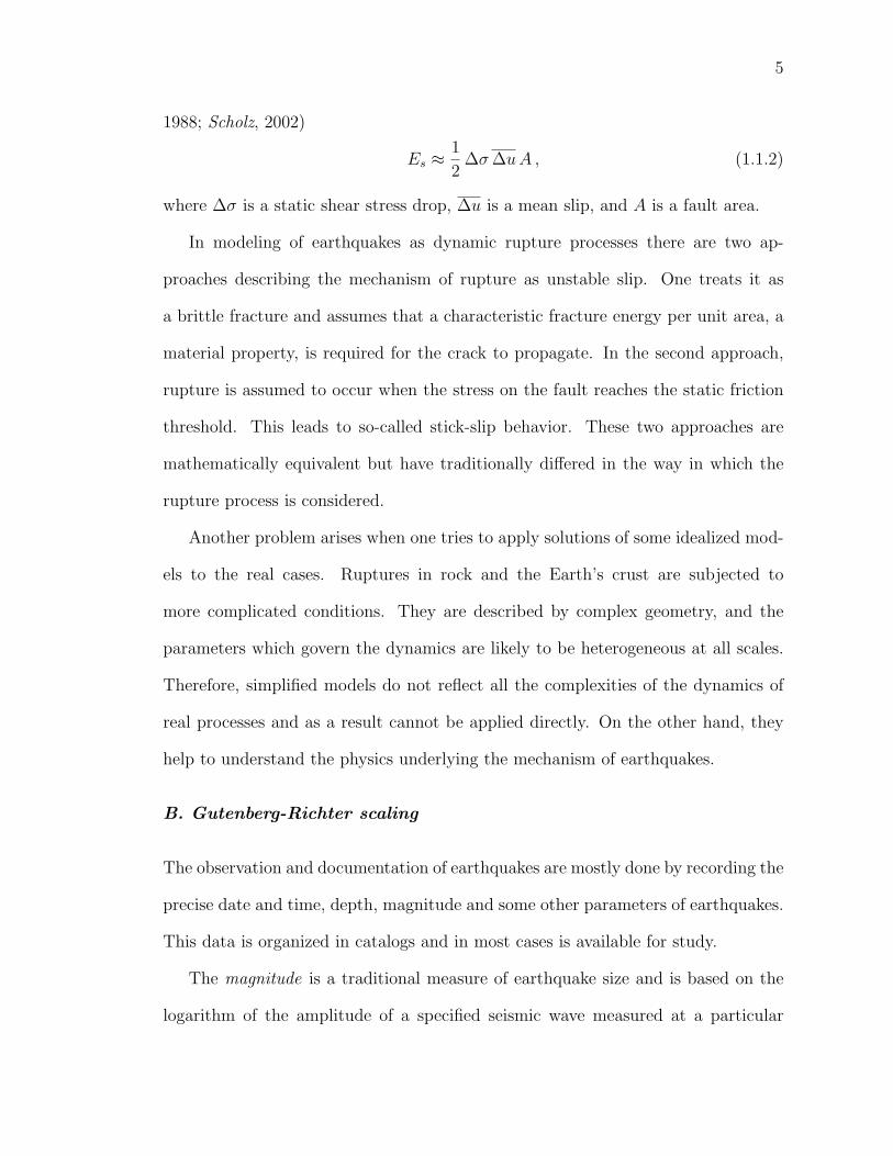
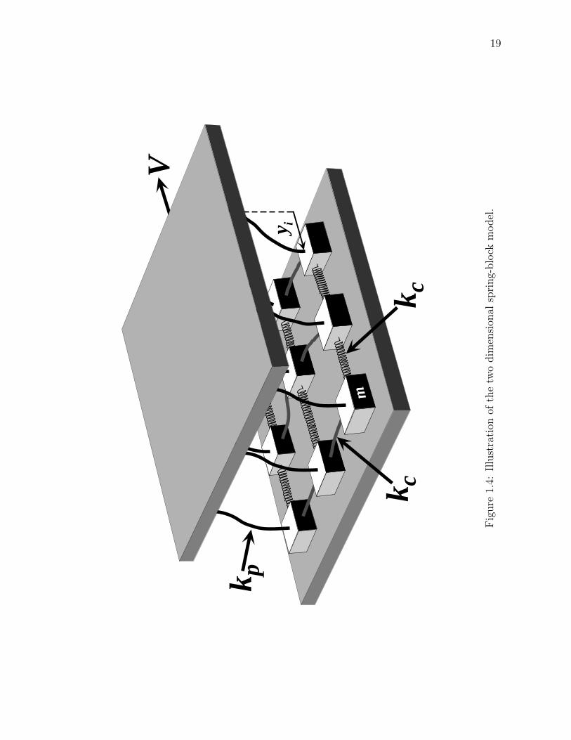
The two-dimensional version of the model is shown in Figure 1.4. The network

of blocks is connected by elastic springs with spring constant Kc and placed between

two plates one of which remains fixed (lower plate) and the other one (driver plate)

moves with constant relative velocity V (analogous to the driving of tectonic plates).

The blocks are allowed to glide on the surface of the fixed plate and different friction

laws can be assigned. Each block is also connected to the driver plate by a set of

springs with spring constant Kp. By specifying the static-dynamic type of friction

18

the motion of each block is made up of slip events. When the force acting on

the block exceeds the maximum static friction the block slips. This may initiate

the movement of nearest-neighbor blocks which in turn may initiate the movement

of next-nearest-neighbor blocks and so on. This process creates avalanches in the

system and is one of the fascinating properties of all these models. These avalanches

are identified with earthquakes.

A continuum approach to the one dimensional version of the spring-block model

was used by Carlson and co-authors (Carlson and Langer, 1989a; Carlson et al.,

1991; Carlson et al., 1994;). The model is described by a massive wave equation

which can be obtained from the equation of motion for each individual block in the

limit a → 0, where a is an equilibrium distance between neighbor blocks (Carlson

and Langer, 1989b; Carlson, 1991). The key nonlinearity in this equation is asso-

ciated with the stick-slip velocity-weakening friction force at the interface between

tectonic plates. They found that magnitude distribution of a purely deterministic,

homogeneous version of the model in the limit of a very long fault and infinitesimally

slow driving rates is consistent with the Gutenberg-Richter law for smaller localized

events, while larger delocalized events do not follow this scaling. The crossover from

smaller events to large ones is identified with a correlation length describing the

transition from localized to delocalized events. Despite a rich and complex behavior

the model does not produce all the features of earthquake dynamics. For example,

it does not contain a mechanism for aftershocks. A generalization of the model by

the introduction of plastic creep in addition to rigid sliding was given by Hahner and

Drossinos (1998, 1999). They found velocity-strengthening and velocity-softening

regimes in the model. Muratov (1999) showed that the Burridge-Knopoff model with

the Coulomb friction law admits solutions in the form of self-sustained shock waves

19

k c

m

V

y i

k p

k c

Fig

ure

1.4:

Illu

stra

tion

ofth

etw

odim

ensi

onal

spri

ng-

blo

ckm

odel

.

20

travelling with constant speed which depends only on the amount of accumulated

stress in front of the wave.

Nakanishi (1990) introduced a cellular automaton version of the one-dimensional

Burridge-Knopoff spring block model. It is interesting to mention here that he found

a critical behavior in the model consistent with Gutenberg-Richter scaling law which

is a pretty rare case among one-dimensional systems.

Another approach was suggested by Olami et al. (1992). They introduced a

continuous cellular automaton in which a level of conservation is a model parame-

ter. The model can be mapped into a two-dimensional version of Burridge-Knopoff

spring-block model and displays the Gutenberg-Richter scaling over a very wide

range of conservation levels (Olami et al., 1992; Olami and Christensen, 1992; Chris-

tensen and Olami, 1992). The scaling exponent in the distribution of avalanche sizes

(b value in Gutenberg-Richter scaling) is no longer universal but depends on the level

of conservation. However, several recent studies cast doubt upon the scaling behav-

ior of the model in a nonconservation regime (Broker and Grassberger, 1997; de

Carvalho and Prado, 2000). An extension of the Burridge-Knopoff model to include

aftershocks has been given by Hergarten and Neugebauer (2002). Some modifica-

tions of the original Olami-Feder-Christensen model were also studied (Hainzl et al.,

1999; Braun and Roder, 2002).

Chaotic behavior in a pair of coupled spring-blocks was found by Huang and

Turcotte (1990, 1992) for some values of model parameters. It is interesting to

note that chaotic behavior in the model requires some asymmetry in the problem.

The dynamics of the model are pretty much similar to the behavior of the logis-

tic map with the period-doubling route to chaos and positive Lyapunov exponents

(Narkounskaia et al., 1992).

21

Different versions of the spring-block model were extensively used in the modeling

of the real fault systems (Rundle, 1988a, 1988b, 1988c; Shaw et al., 1992; Rice, 1993;

Ben-Zion and Rice, 1993; Rundle et al., 2001).

C. Forest-fire model

Another model introduced to illustrate SOC behavior was the forest-fire model.

The original version of the model was proposed by Bak et al. (1990) as a model

for turbulence and the spread of natural fires. In this model each site of the d-

dimensional grid can be in three possible states: green tree, burning tree, or ash.

The evolution of the model is defined as follows. A burning tree starts an avalanche

of fire and ignites all green neighbor trees. During the next time step all burning

trees turn into ash. New trees are planted with some probability p 1 which is a

control parameter in the model. The system is updated parallel according to the

above rules. Simulations of the model on large lattices (Grassberger and Kantz, 1991)

showed that the dynamics are quite different from that suggested previously by Bak

et al. (1990). The system in two dimensions develops spiral patterns (fire fronts)

which propagate with finite mean velocity v for any p, and the typical distance ξ

between fire fronts (the characteristic length scale) as well as the time T between

two passings of a front scales as 1/p. The latest simulations of the model (Broker

and Grassberger, 1997) revealed that the model is not critical in two dimensions but

shows anomalous scaling in three and four dimensions.

To overcome difficulties with the two dimensional forest-fire model described

above Drossel and Schwabl (1992) added a second control parameter, the firing

frequency f , in the model. This parameter defines a probability that a green tree

catches fire during one time step. The extensive numerical simulations of the model

(Drossel and Schwabl, 1992, 1993; Clar et al., 1994, 1996, 1997) and a dynamically

22

driven renormalization group approach (Loreto et al., 1995, 1996) showed that the

model becomes critical in the limit of a double time scale separation. This implies

that the time scale over which a cluster of green trees is burnt is much smaller than

the growth rate of planting new green trees which, in turn, is much smaller than the

time scale over which a lighting event occurs. This time scale separation is defined

by the following double limit

f

p→ 0 , p→ 0 . (1.1.16)

The dynamics of the model depend only on the ration f/p, but not on f and

p separately. In the simulations, the condition (1.1.16) is most easily realized by

burning forest clusters instantaneously, i.e. during one time step. This extreme limit

of the SOC forest-fire model has been invented independently by Henley (1993).

The comparison of the model and behavior of natural forest fires was given

by Malamud et al. (1998). It was found that actual forest fires show reasonable

power-law scaling over a wide range of magnitudes, which is consistent with the

behavior predicted by the model. However, the critical slope of these distributions

is somewhat higher than the one obtained in the model.

1.1.3 Fracture of solids and statistical physics

A. Damage mechanics

The nonelastic behavior of solid materials is characterized by a wide range of pro-

cesses; examples include decohesion between inclusions, accumulation of dislocations

leading to the nucleation of microcracks, debonding of fibers and matrix in composite

materials, etc. This irreversible behavior is often referred to as damage (Kachanov,

1986; Lemaitre and Chaboche, 1990; Krajcinovic, 1996). The thermally activated

23

creep processes (diffusion and dislocation creep) which are responsible for mantle

convection also involve damage. Plastic deformation of ductile materials beyond a

threshold and the rupture of brittle materials are other examples of damage. In

this paper we will concentrate our attention on the irreversible deformation of solids

with the object of better understanding the deformation of the earth’s crust.

The brittle failure of a solid is certainly a complex phenomenon that has received

a great deal of attention from engineers, geophysicists, and physicists. A limiting

example of brittle failure is the propagation of a single fracture through a homoge-

neous solid. However, this is an idealized case that requires a preexisting crack or

notch to concentrate the applied stress. Even the propagation of a single fracture

is poorly understood because of the singularities at the crack tip (Freund, 1990).

In most cases, the fracture of a homogeneous brittle solid involves the generation

of microcracks. Initially these microcracks are randomly distributed, as their den-

sity increases they coalesce and localize until a through-going rupture results. This

process depends upon the heterogeneity of the solid.

Many experiments on the fracture of brittle solids have been carried out. In terms

of rock failure, the early experiments by Mogi (1962) were pioneering. Acoustic

emissions (AE) associated with microcracks were monitored, power-law frequency-

magnitude statistics were observed for the AE. When a load was applied very rapidly,

the time-to-failure was found to depend on the load. Many other studies of this type

have been carried out. Otani et al. (1991) obtained the statistical distribution of the

life times with constant stress loading for carbon fibre-epoxy microcomposites. Jo-

hansen and Sornette (2000) studied the rupture of spherical tanks of kevlar wrapped

around thin metallic linens and found a power-law increase of AE prior to rupture.

Guarino et al. (1998, 1999) studied the failure of chipboard and fiberglass pan-

24

els. They obtained power-law increases in AE prior to rupture and a systematic

dependence of failure times on stress level.

In engineering applications, problems associated with brittle rupture are often

studied using continuum damage mechanics (Lemaitre and Chaboche, 1990; Kraj-

cinovic, 1996). A damage variable α is introduced that is a measure of deviations

from linear elasticity. The evolution of damage is specified by a rate equation. There

is a close analogy between the damage model and the fiber-bundle model. In the

dynamic fiber-bundle model a prescribed statistical distribution of times to failure

for the fibers is introduced as a function of fiber stress. When a fiber fails the stress

on the fiber is redistributed to other fibers. The damage variable α in the damage

model is directly related to the fraction of fibers that have failed in the fiber-bundle

model (Turcotte et al., 2002).

A characteristic of the rupture of brittle materials, as described above, is the

time delay between the application of a stress and the rupture. In the earth’s brittle

crust, the aftershock sequences following all earthquakes are examples of this type of

delay. When a rupture occurs on a fault there is a redistribution of stress around the

fault. Some regions have a reduction in stress (stress shadows), and other regions

have an increase in stress (stress halos). Since the total stored elastic energy must

decrease, the integrated reduction of stress is greater than the integrated increase.

Nevertheless, the regions of increased stress are significant and it is these regions

where aftershocks occur (both on the fault that initially ruptured and on adjacent

faults) (Dieterich, 1994).

While there are important similarities between the fracture of a pristine rock

and an earthquake rupture, there are also important differences. The fracture of a

pristine rock is an irreversible process. However, earthquake ruptures occur repet-

25

itively on preexisting faults and, between earthquakes, faults heal. If the Earth’s

crust, prior to a major earthquake, behaved like the fracture of a pristine rock,

there would be a systematic increase in regional seismicity before a major earth-

quake. The rate of occurrence of small earthquakes in a seismogenic zone is nearly

constant (Turcotte, 1999). However, there is accumulating evidence that there is

an increase in the number of intermediate-sized earthquakes prior to a large earth-

quake (Rundle et al., 2000). The repetitive nature of earthquakes, as well as their

power-law scaling, have led some authors to argue that seismicity is an example of

self-organized criticality (Bak et al., 1987, 1988, 1989). It is certainly reasonable to

hypothesize that the Earth’s crust is in a “damaged” state. Evidence of this dam-

age is the continuous occurrence of small earthquakes that satisfy Gutenberg-Richter

frequency-magnitude scaling.

B. Phase changes and rupture

Statistical physicists have related brittle rupture to liquid-vapor phase changes in

a variety of ways. Buchel and Sethna (1997) have associated brittle rupture with

a first-order phase transition. Similar arguments have been given by Zapperi et al.

(1997) and Kun and Herrmann (1999). On the other hand Sornette and Andersen

(1998), Sornette (2000), and Gluzman and Sornette (2001) argue that brittle rupture

is analogous to a critical point phenomena, not to a first-order phase change. They

associated observed power-law scaling in brittle failure experiments with a critical

point (a second-order phase change). A number of authors have considered brittle

rupture in analogy to spinodal nucleation (Selinger et al., 1991; Rundle et al., 1996,

1999, 2000; Zapperi et al., 1999).

In order to provide a basis for discussing material failure as a phase change pro-

cess, we first discuss the phase diagram for the coexistence of the liquid and vapor

26

A

1

1 20

B

D E

J

GH

C

S S'

Liquid+VapourLiquid Vapour

F

P/Pc

V/Vc

I

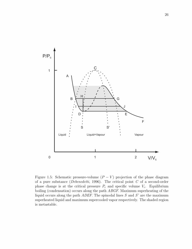
Figure 1.5: Schematic pressure-volume (P − V ) projection of the phase diagramof a pure substance (Debenedetti, 1996). The critical point C of a second-orderphase change is at the critical pressure Pc and specific volume Vc. Equilibriumboiling (condensation) occurs along the path ABGF. Maximum superheating of theliquid occurs along the path ADEF. The spinodal lines S and S’ are the maximumsuperheated liquid and maximum supercooled vapor respectively. The shaded regionis metastable.

27

phases of a pure substance. A schematic pressure-volume projection of a phase di-

agram is illustrated in Figure 1.5 (Debenedetti, 1996). We consider the boiling of a

liquid initially at point A in the figure. The pressure is decreased isothermally until

the phase change boundary is reached at point B. In thermodynamic equilibrium

the liquid will boil at constant pressure and temperature until it is entirely a vapor

at point G. Further reduction of pressure will result in the isothermal expansion of

the vapor along the path GF. However, it is possible to create a metastable, super-

heated liquid at point B. If bubbles of vapor do not form, either by homogeneous

or heterogeneous nucleation, the liquid can be superheated along the path BD. The

point D is the intersection of the liquid P–V curve with the spinodal curve S. It is

not possible to superheat the liquid beyond this point. If the liquid is superheated to

the vicinity of point D, explosive nucleation and boiling will take place. If the pres-

sure and temperature are maintained constant during this highly nonequilibrium

explosion, the substance will follow the path DE to the vapor equilibrium curve

GF. If the explosion occurs at constant volume and temperature, the pressure will

increase as the substance follows the path DH to the equilibrium boiling line BG.

Any horizontal path between the superheated liquid BD and vapor GE is possible.

An example is the path IJ. The entire shaded region is metastable. A point on a

horizontal line, for example IJ, is determined by the “wetness” of the liquid-vapor

mixture, the mass fraction that is liquid. At point I the mass fraction of liquid is 1,

at point J the mass fraction of liquid is 0. Which path is followed in the metastable

region is determined by the physics of the bubble nucleation process (Debenedetti,

1996).

We next apply the concept of phase change to the brittle fracture of a solid. For

simplicity we will discuss the failure of a sample of area a under compression by a

28

force F. The state of the sample is specified by the stress σ = F/a and its strain

ε = (L−L0)/L0 (L length, L0 initial length). The dependence of the stress on strain

is illustrated schematically in Figure 1.6. At low stresses we assume that Hooke’s

law is applicable so that

σ = E0 ε , (1.1.17)

where E0 is Young’s modulus, a constant.

We hypothesize that a pristine brittle solid will obey linear elasticity for stresses

in the range 0 ≤ σ ≤ σy, where σy is a yield stress. From (1.1.17) the corresponding

yield strain εy is given by

εy =σy

E0

. (1.1.18)

If stress is applied infinitely slowly (to maintain a thermodynamic equilibrium), we

further hypothesize that the solid will fail at the yield stress σy. The failure path

ABG in Figure 1.6 corresponds to the equilibrium failure path ABG in Figure 1.5.

This is equivalent to the perfectly plastic behavior.

If an elastic solid is loaded very rapidly with a constant stress σ0 > σy applied

instantaneously as shown in Figure 1.6, path ABI, damage will occur along the stress

path IJ until the solid fails. This behavior is analogous to the constant pressure

boiling that occurs along the path IJ in Figure 1.5.

Alternatively the elastic solid could be strained very rapidly with a constant

strain ε0 > εy applied instantaneously as shown in Figure 1.6. In this case damage

will occur along the constant strain path IH until the stress is reduced to the yield

stress σy. This behavior is analogous to the constant volume boiling that occurs

along the path parallel to DH in Figure 1.5.

When the stress on a brittle solid is increased at a constant finite value we

hypothesize that linear elasticity (1.1.17) is applicable in the range 0 ≤ σ ≤ σy.

29

σ/σy

ε/εy

A

B1

2

1 2

I

H

J

G

F

E

0

σ0 /σy

ε0 /εy

α = 0

α = 0.25

α = 0.5

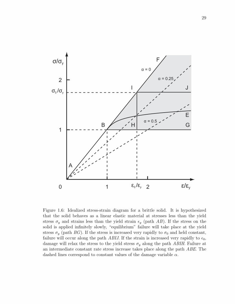
Figure 1.6: Idealized stress-strain diagram for a brittle solid. It is hypothesizedthat the solid behaves as a linear elastic material at stresses less than the yieldstress σy and strains less than the yield strain εy (path AB). If the stress on thesolid is applied infinitely slowly, “equilibrium” failure will take place at the yieldstress σy (path BG). If the stress is increased very rapidly to σ0 and held constant,failure will occur along the path ABIJ. If the strain is increased very rapidly to ε0,damage will relax the stress to the yield stress σy along the path ABIH. Failure atan intermediate constant rate stress increase takes place along the path ABE. Thedashed lines correspond to constant values of the damage variable α.

30

At stresses greater than the yield stress, σ > σy, damage occurs in the form of

microcracks. This damage results in accelerated strain and a deviation from linear

elasticity. A typical failure path ABJ is illustrated in Figure 1.6. In order to quantify

the deviation from linear elasticity the damage variable α has been introduced in

the strain-stress relation

σ = E0 (1− α) ε . (1.1.19)

When α = 0, (1.1.19) reduces to (1.1.17) and linear elasticity is applicable; as α→ 1

(ε → ∞) failure occurs. States in the stress-strain plot, Figure 1.6, corresponding

to α = 0, 0.25, and 0.5 are shown by dashed lines.

C. Scaling and universality

Scaling in static critical phenomena was independently developed by several au-

thors, including Widom, Domb and Hunter, Kadanoff, Patashinskii and Pokrovskii,

and Fisher (for reviews see Kadanoff et al. 1967; Fisher 1967; Patashinskii and

Pokrovskii 1979; Stanley 1971).

The scaling hypothesis for functions that describe the behavior of the system

(the function could be the thermodynamic potential or the equation of state) states

that asymptotically close to the critical point the singular part of this function is a

generalized homogeneous function (Stanley, 1971). This property can be expressed

mathematically as follows

F(λ1/α x, λ1/β y, . . .) = λF(x, y, . . .) , (1.1.20)

where λ is any positive scaling constant, x and y are thermodynamic fields such as

temperature, magnetic field, etc., and α and β are critical indices. In the case of a

homogeneous function of one variable (1.1.20) takes the form

F(λ1/α x) = λF(x) . (1.1.21)

31

This equation has a simple solution in the form of a power law

F(x) = C xα , (1.1.22)

which can be verified by direct substitution.

Scaling or scale invariance is the fundamental property that plays an essential

role in modern statistical physics. In the geometrical domain the notion of scale

invariance led to the discovery of fractals (Mandelbrot, 1982).

Another pillar of modern statistical mechanics is the hypothesis of universality

which states that the critical behavior of most systems can be divided into universal-

ity classes (Stanley, 1971; Sornette, 2000). Each universality class is characterized

by the same set of critical indices which were introduced in (1.1.20). This is a very

powerful tool which allows us to describe real systems by simplified mathematical

models. The model does not need to be too complicated and describe every detail of

the real system but instead it needs only to incorporate fundamental properties of

the real system such as dimensionality, symmetry, the type of interaction between

the components of the system (long range, short range), and some other characteris-

tics. For example, the three-dimensional quantum Heisenberg model describes very

accurately the critical behavior of wide class of ferromagnets.

We believe that these ideas of scale invariance and universality are crucial in

understanding the physics of earthquakes. The manifestation of the scale invariant

behavior of earthquakes is the Gutenberg-Richter law (1.1.7) and the example of the

model which simulates the behavior of the single fault is the spring-block model.

32

1.2 Martian figure and internal composition

1.2.1 Topography, gravity field, and planetary interior

Correlations between topography, gravity, and areoid can provide important con-

straints on the structure and tectonic evolution of planetary bodies (Heiskanen and

Meinesz, 1958; Heiskanen and Moritz, 1967; Esposito et al., 1992; Spohn, 1998).

The improved topography (Smith et al., 1999a) and gravity (Smith et al., 1999b)

obtained by the Mars Global Surveyor (MGS) spacecraft allow new opportunities

for applying these correlations to Mars.

To a first approximation, the shape (figure) of a planetary body is determined

by hydrostatic considerations. The interiors of planetary bodies are sufficiently hot

that they can flow (creep) on geological time scales until they are in near hydro-

static equilibrium. Without planetary rotation, this equilibrium is a self-gravitating

sphere. For planetary bodies with significant rotation, such as Mars and the Earth,

hydrostatic equilibrium requires polar flattening and an equatorial bulge (Jardetzky,

1958; Kopal, 1960).

Deviations from a hydrostatic shape for a planet can have two origins. The

first are static deviations supported by the rigidity of the planetary shell, the elastic

lithosphere. The second are dynamic deviations supported by the stresses associated

with mantle convection. For the Earth, the global figure is essentially hydrostatic.

Variations in topography are attributed almost entirely to variations in the thickness

of the crust and lithosphere.

On planetary bodies, the elastic lithospheric shell provides support for surface

volcanic and tectonic loads. On the Earth, this support can be explained by the

bending rigidity of the elastic lithosphere. Mars, however, is a relatively small

33

planetary body and it is necessary to also include the membrane (shell) stresses

in the elastic lithosphere when considering the support of loads. The appropriate

static support analysis for the Tharsis load on Mars has been given by a number of

authors (Turcotte et al., 1981; Willemann and Turcotte, 1982; Banerdt et al., 1982;

Solomon and Head, 1982; Comer et al., 1985; Sleep and Phillips, 1985; Zuber and

Smith, 1997). These analyses predict the surrounding areoid low and the antipodal

areoid high.

It has also been proposed that a significant component of the topography of the

Tharsis rise is dynamic in origin. An active mantle plume beneath Tharsis would

be expected to have an associated domal uplift (Kiefer et al., 1996; Breuer et al.,

1996, 1997, 1998; Harder, 1998, 2000; Matyska et al., 1998; Harder and Christensen,

1996). The Hawaiian swell is an example of an uplift on the Earth that is associated

with a mantle plume.

The current studies of Mars interior are constrained by the only knowledge of

its gravity field and the planetary shape and the cosmochemical data obtained from

the SNC (Shergotty, Hakhla, and Chasigny) meteorites. This data is not enough

to construct the unique model of the Martian internal structure. The placement of

seismometers during the future missions to Mars will change this situation. Mean-

while, using the existing data we only can answer some general questions, such as,

the existence of the dense core or to put constraints on the thickness of the elastic

lithosphere and crust.

The recent missions of Mars Pathfinder (MP) and MGS spacecrafts significantly

improved our knowledge of the fundamental geodetic parameters of the planet. From

the values of the mass and mean planetary radius it is possible to obtain the mean

planetary density. These values can be found in Table 4.1. A constraint on the

34

internal mass distribution can be deduced from the values of its principal moments

of inertia. The latest estimates by Folkner et al. (1997) using the data from the MP

spacecraft (the Doppler frequency shift), allowed them to obtain an improved rate

of secular precession and periodic nutation of the spin axis. From this data they

estimated the polar moment of inertia of the Mars C/MR2 = 0.3662± 0.0017.

This value of C/MR2 and the geochemical analyses suggest that Mars has

a dense core with a radius somewhere between 1300 and 1900 km and density

6800 ± 700 kg m−3. The absence of an internal magnetic field at present and the

strong magnetic anomalies detected by the MGS spacecraft in the southern hemi-

sphere suggest that Mars had a vigorously convected core during the first 0.5–1 Gyr

which solidified afterward. Some structural models based on geochemical arguments

suggest that the core has a high sulfur content and is composed mostly of Fe, Ni,

and FeS (Sohl and Spohn, 1997).

The mantle composition is believed to be similar to the Earth. For example,

Longhi et al. (1992) divided the Martian mantle into an upper olivine-rich part

with density 3520 kg m−3, a transition zone composed of silicate-spinel with density

3720 kg m−3, and a lower perovskite-rich zone with density 4170 kg m−3. Two

other models were also considered recently by Sohl and Spohn (1997). The first

model was constrained by the upper limit on C/MR2 = 0.366 and the second model

was constrained by the chondritic Fe/Si ration of 1.71. It was found that it is not

possible to satisfy both constraints simultaneously.

1.2.2 Hydrostatic considerations

The simplest approach to the rotational distortion of a planetary body is to assume

that it is a rotating fluid. This is the hydrostatic approximation. The figure is also an

35

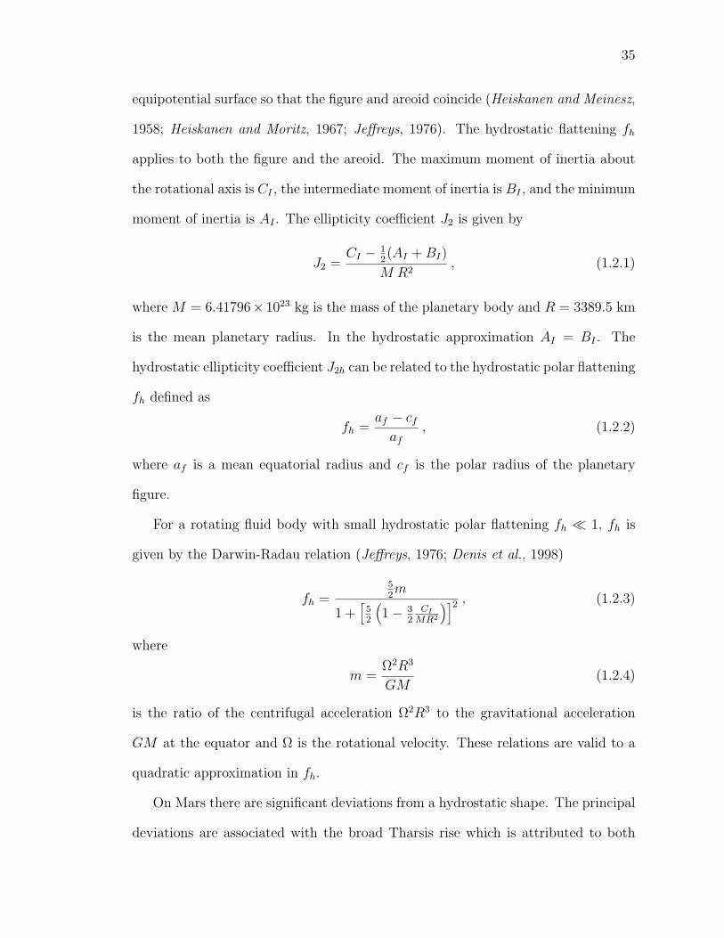
equipotential surface so that the figure and areoid coincide (Heiskanen and Meinesz,

1958; Heiskanen and Moritz, 1967; Jeffreys, 1976). The hydrostatic flattening fh

applies to both the figure and the areoid. The maximum moment of inertia about

the rotational axis is CI , the intermediate moment of inertia is BI , and the minimum

moment of inertia is AI . The ellipticity coefficient J2 is given by

J2 =CI − 1

2(AI +BI)

M R2, (1.2.1)

where M = 6.41796× 1023 kg is the mass of the planetary body and R = 3389.5 km

is the mean planetary radius. In the hydrostatic approximation AI = BI . The

hydrostatic ellipticity coefficient J2h can be related to the hydrostatic polar flattening

fh defined as

fh =af − cfaf

, (1.2.2)

where af is a mean equatorial radius and cf is the polar radius of the planetary

figure.

For a rotating fluid body with small hydrostatic polar flattening fh 1, fh is

given by the Darwin-Radau relation (Jeffreys, 1976; Denis et al., 1998)

fh =52m

1 +[

52

(1− 3

2CI

MR2

)]2 , (1.2.3)

where

m =Ω2R3

GM(1.2.4)

is the ratio of the centrifugal acceleration Ω2R3 to the gravitational acceleration

GM at the equator and Ω is the rotational velocity. These relations are valid to a

quadratic approximation in fh.

On Mars there are significant deviations from a hydrostatic shape. The principal

deviations are associated with the broad Tharsis rise which is attributed to both

36

volcanic and tectonic processes and rises up to 10 km above its surroundings (Carr,

1981). The topography of the Tharsis rise is supported by bending and shell stresses

in the elastic lithosphere. There are large gravity and areoid anomalies that are

directly correlated with topography. Also associated with Tharsis are a surrounding

areoid low and an areoid high at its antipode.

37

1.3 Outline

In this dissertation I report on the modeling of some aspects of earthquake physics

and the study of the thickness of the Martian crust and elastic lithosphere. The

thesis is organized as follows:

1) In Chapter 2, we study numerically and analytically two models of self-orga-

nized criticality; Height-arrow model and Eulerian walker model.

2) Chapter 3 presents our results on the application of damage mechanics to

earthquake physics. In particularly, we compare the microscopic fiber-bundle

model for failure with the macroscopic damage model for failure in a simple

geometry. We also consider and solve several models of deformation of solids

and discuss their application to earthquake processes.

3) Chapter 4 is devoted to the study of the Martian crust and elastic lithosphere.

We use recent data for gravity and planetary shape obtained from the Mars

Global Surveyor spacecraft to estimate the thickness and density of the plan-

etary crust and elastic lithosphere.

4) Chapter 5 will conclude the thesis and summarize our results.

5) The appendixes elaborate on some techniques and methods used in studying

the models of self-organized criticality and estimating the thickness of the

Martian crust and elastic lithosphere.

Chapter 2

Models of self-organized criticality

To illustrate the phenomenon of self-organized criticality (SOC) (Bak et al., 1987,

1988) a wide range of cellular automata such as sand piles, rice piles and forest fires,

have been proposed (Bak et al., 1987, 1988; Frette et al., 1996; Drossel and Schwabl,

1992). They assume a system consisting of a large number of elements. The energy

being randomly added to the system is redistributed then over the degrees of freedom

by a kind of nonlinear diffusion. This is realized by avalanchelike processes which

carry the added energy out of the system. As a rule, the system spontaneously

evolves towards the critical state free of any characteristic length and time scale.

In this state, probabilistic distributions of quantities characterizing the statistical

ensemble exhibit the power-law behavior.

Which features of the SOC dynamics are responsible for the existence of a dy-

namic attractor in complex systems? What are the origins of the scaling and self-

similarity in the stationary state? To answer these questions, one should investigate

nonlinear diffusion in the SOC models and study the structure of avalanches. The

difficulties encountered here arise from the complexity of dynamic processes in the

strongly correlated SOC systems. Up to now, the most analytically tractable model

38

39

has been the Abelian sandpile model (ASM) (Dhar, 1990, 1999). Due to its sim-

ple algebraic structure, the detailed description of the SOC state of ASM has been

given, and some critical exponents have been found (Majumdar and Dhar, 1991;

Priezzhev, 1994; Ivashkevich et al., 1994; Priezzhev et al., 1996a).

Recently, a new model has been proposed which is called the Eulerian walkers

model (EWM) (Priezzhev et al., 1996b). In a sense, this model is even more el-

ementary than ASM as it deals with a single moving particle. The dynamics of

this model is driven by a walking particle. The motion of a particle is affected by

the medium, and in its turn affects the medium inducing long range correlations in

the system. If the walk occurs in a closed system, it continues infinitely long and

eventually gets self-organized into Eulerian trails (Harary and Palmer, 1973). If a

system is open, the particles can leave the system and new particles drop time after

time. In this case, the system evolves to the critical state similar to that in ASM.

By analogy with ASM, the avalanches in EWM have been introduced (Priezzhev,

1998) as periods of reconstruction of recurrent states, after they have been broken

by an added particle.

Another aspect of EWM is the possibility to look at non-trivial diffusion laws

and their change under the self-organization. In contrast to the self-avoiding walk

where an infinitely long memory is due to exclusion of multiple visits of lattice sites,

EWM presents an alternative way to introduce memory effects. The visited sites are

not forbidden for the next visits but a prescription for the next step is changed after

each visit. As a result, EWM evolves to the critical state where the deterministic

walk is characterized by the simple diffusion law.

Like most of problems of the graph theory, EWM admits a simple “real life”

interpretation. A treatment of EWM as the model of the distribution of goods in a

40

spatially extended market is given in section II.

In this Chapter, we also study the self-organizing height-arrow (HA) model

(Priezzhev et al., 1996; Shcherbakov and Turcotte, 2000). It combines features of the

Abelian sandpile model (ASM) model (Dhar, 1990, 1999; Ivashkevich and Priezzhev,

1998) and self-organizing Eulerian walkers model (EWM) (Priezzhev et al., 1996;

Shcherbakov et al., 1997; Povolotsky et al., 1998). The model is a cellular automaton

defined on any connected undirected graph. In this model, each site of the graph

can be occupied by a particle or can be empty. Addition of the particle to an oc-

cupied site makes it unstable and causes it to topple. The site becomes empty and

the particles are transferred to the nearest neighbors. The redistribution of parti-

cles from an unstable site is governed by the second site variable, an arrow. Each

outgoing particle from the toppled site turns the arrow by a prescribed angle and

the new direction of the arrow determines the nearest neighbor site for this particle.

The sequence of turns of arrows can be periodic with period T or nonperiodic with

T = ∞. During this period T the redistributions of particles (turns of an arrow) for

the given site form a minimal nonperiodic sequence. The ASM model can be consid-

ered with the period T = 1 as if we place arrows at each site of the lattice then each

toppling of a given site restores the initial arrow direction. In the two-state Manna

model the sequence of topplings at each site is stochastic without any periodicity,

therefore, one can put T = ∞ for this model. For simplicity, it is convenient to

assign the same period T for all sites of the lattice. Thus, one can define the HA

models with increasingly complicated dynamic rules. These pseudo-random models

tend to the random ones for large T →∞.

41

2.1 Self-organizing height-arrow model

2.1.1 The model on the square lattice.

The HA model we consider is defined as follows (Priezzhev et al., 1996; Shcherbakov

and Turcotte, 2000). Each site i of the two-dimensional L × L square lattice is

assigned a height variable zi ∈ 0, 1, ... and an arrow directed north (N), east (E),

south (S) or west (W) from i. We start with an arbitrary initial configuration of

heights and arrows on the lattice. Initially, we drop a particle on the randomly

chosen site i. The succeeding evolution of the system is determined by the following

rules. We increase the height variable at the site i by 1, zi → zi + 1. If the site i is

already occupied by one or more particles, it topples (zi → zi − 2). To redistribute

the particles from the toppled site i among its nearest neighbors, we first rotate the

arrow according to a prescribed rule and then move the first particle along the new

direction of the arrow. Then, we turn the arrow again and move the second particle.

After that, the arrow points in the direction of the last transferred particle from the

toppled site. Thus, each particle from the toppled site turns the arrow and a new

direction of the arrow points to the nearest neighbor site where the particle will be

transferred. In this work we consider the HA model with open boundary conditions.

If the new direction of an arrow points out of the lattice the toppled particle leaves

the system, thus, providing dissipation of energy in the system.

For the given period T = 2, there are only two non-equivalent sequences of

turns of the arrow at the given site which preserve the model from being directed.

Hereafter, these sequences of turns will be distinguished as N-E-S-W-N and N-S-W-

E-N. After each turn the new direction of the arrow points to the neighbor sites to

which we will transfer particles at the next time step. This process continues until a

42

stable configuration is reached. The sequence of topplings of unstable sites forms an

avalanche which propagates through the lattice and may reach boundaries. After

an avalanche ceases, we go on by adding a new particle and so on.

A given configuration of the model is a set of directions of arrows and heights.

The total number of them is 8L×L. During the evolution of the system the arrow

at any site might be only in two positions due to the fact that the two subsequent

topplings of the site restore the initial position of the arrow. Therefore, the set of

configurations of the model falls into 2L×L equivalent classes which are determined by

initial configurations of arrows. The HA model is Abelian in terms of commutation

of topplings (Priezzhev, 1998).

Starting from an arbitrary configuration of arrows and occupied sites, the model

evolves through transient states into a dynamic attractor which is critical. This

attractor is identified with the SOC state as different dynamic characteristics of

the model show power-law tails in their distributions. The model being in the

SOC state passes from one allowed stable configuration to another by avalanche

dynamics. This critical state has been investigated in detail by Priezzhev (1998).

He defined operators corresponding to addition of a particle at a randomly chosen

site and showed that they commute with each other. The algebra of these operators

is used to calculate the number of allowed configurations of a given class in the SOC

state. This number is shown to be equal to the determinant of the discrete Laplacian

matrix ∆ of the square lattice. To check the given configuration to be allowed in the

SOC state the modification of the burning algorithm was also introduced (Priezzhev,

1998).

43

2.1.2 Numerical results.

In order to investigate the static properties and avalanche dynamics in the HA

model, we have carried out numerical simulations. We consider square lattices of

size L× L with open boundary conditions and L ranging from 64 up to 1024. The

HA model has been studied for two different types of dynamics (N-E-S-W-N and

N-S-W-E-N) of turns of arrows and various initial conditions.

Starting from an arbitrary distribution of occupied sites and certain initial di-

rections of arrows, the finite system evolves into a stationary state. In this state we

have measured the time average density 〈p(z = 1)〉 and critical exponents for distri-

butions of avalanches by mass (s), area (a) and duration (t). The mass s is defined

to be the total number of topplings in an avalanche whereas the area a is defined

as the number of distinct sites visited by an avalanche. A single time step considers

a simultaneous topplings of all unstable sites. The duration t of an avalanche is

the number of these steps. For a more detailed description of the structure of an

avalanche it is also useful to define a linear extent (diameter) of the avalanche cluster

via a radius of gyration (r). We also measured the corresponding fractal dimensions

γxy, where x, y = s, a, t, r.

As is shown in Figure 2.1, the steady state is reached by the model after about

100 000 avalanches on the square lattice of linear size L = 512 for the system which

is initially has no particles and with a random initial distribution of arrows. In this

simulation, we were recording the average density 〈p(z = 1)〉 of occupied sites at

each time when the avalanche ends.

As has been mentioned in Section 2.1.1, the number of configurations for the

model falls into 2L×L classes depending on the initial configurations of arrows. In

our simulations of the HA model with the N-E-S-W-N dynamics we started from

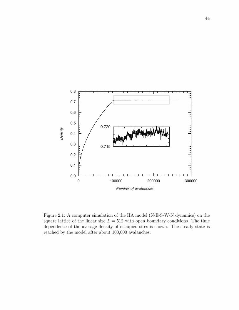
44

0 100000 200000 300000

Number of avalanches

0.0

0.1

0.2

0.3

0.4

0.5

0.6

0.7

0.8

Den

sity

0.715

0.720

Figure 2.1: A computer simulation of the HA model (N-E-S-W-N dynamics) on thesquare lattice of the linear size L = 512 with open boundary conditions. The timedependence of the average density of occupied sites is shown. The steady state isreached by the model after about 100,000 avalanches.

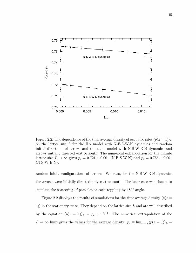
45

0.000 0.005 0.010 0.015

1/L

0.70

0.71

0.72

0.73

0.74

0.75

0.76

<p(z=1)>

N-S-W-E-N dynamics

N-E-S-W-N dynamics

Figure 2.2: The dependence of the time average density of occupied sites 〈p(z = 1)〉Lon the lattice size L for the HA model with N-E-S-W-N dynamics and randominitial directions of arrows and the same model with N-S-W-E-N dynamics andarrows initially directed east or south. The numerical extrapolation for the infinitelattice size L → ∞ gives pc = 0.721 ± 0.001 (N-E-S-W-N) and pc = 0.755 ± 0.001(N-S-W-E-N).

random initial configurations of arrows. Whereas, for the N-S-W-E-N dynamics

the arrows were initially directed only east or south. The later case was chosen to

simulate the scattering of particles at each toppling by 180 angle.

Figure 2.2 displays the results of simulations for the time average density 〈p(z =

1)〉 in the stationary state. They depend on the lattice size L and are well described

by the equation 〈p(z = 1)〉L = pc + c L−1. The numerical extrapolation of the

L → ∞ limit gives the values for the average density: pc ≡ limL→∞〈p(z = 1)〉L =

46

0.721±0.001 (N-E-S-W-N dynamics) and pc = 0.755±0.001 (N-S-W-E-N dynamics).

These values are a little higher in comparison with the stochastic two-state Manna

model (Manna, 1991) (see Table 2.1).

The form of avalanches in the HA model has a layered structure. A typical

avalanche is shown in Figure 2.3 where the number of relaxations in each site is

marked by different scales of gray color. The sites with the same number of re-

laxations form a layer or shell. We have observed that layers group in pairs. In

each pair a larger layer is a connected cluster with holes whereas a smaller one is a

disconnected cluster without holes. Therefore, in the avalanche cluster there are a

very few holes only near the boundary in the first layer where each site topples only

once.

In Figures 2.4, we present the binned distributions of avalanches by mass s, area

a and duration t in a double logarithmic plot for the N-E-S-W-N dynamics and

lattices with different sizes. In these simulations we measure P (x) = N(x)Ntotal

, where

N(x), x = s, a, t, is a number of events of a given size x and Ntotal is the total

number of avalanches. These distributions display a power-law behavior up to a

cutoff which depends on the system size L. Since our simulations are limited by the

lattice size we apply a finite-size scaling analysis (see Appendix A).

To reduce fluctuations in the data, we integrated each distribution over bin

lengths. The exponents γxy, x, y = s, a, t, are measured from the slopes of the

straight parts of the corresponding plots (Figures 2.5). The derived values of expo-

nents are given in Table 2.2.

Plotting binned distributions P (s, L)·Lβs versus s·L−νs and P (a, L)·Lβa versus a·

L−νa on a double logarithmic scale, as is shown in Figures 2.6, 2.7 for different lattice

sizes L, we obtained from finite-size scaling analysis that the best data collapse

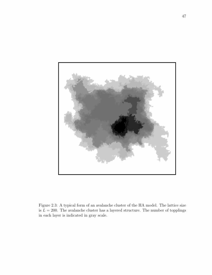
47

Figure 2.3: A typical form of an avalanche cluster of the HA model. The lattice sizeis L = 200. The avalanche cluster has a layered structure. The number of topplingsin each layer is indicated in gray scale.

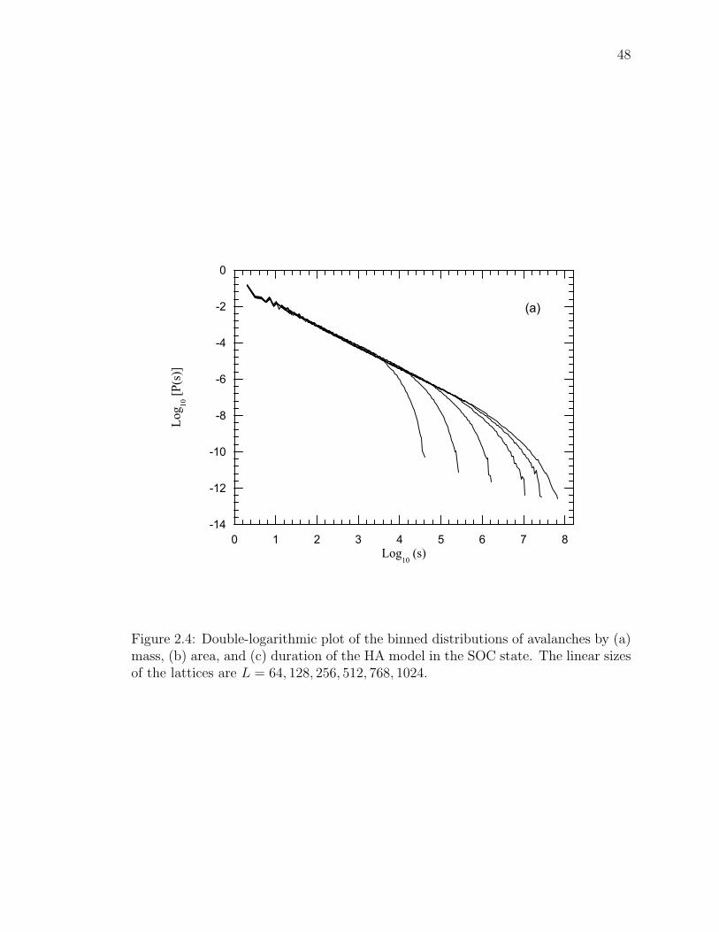
48

0 1 2 3 4 5 6 7 8Log

10 (s)

-14

-12

-10

-8

-6

-4

-2

0

Log 10

[P(s

)]

(a)

Figure 2.4: Double-logarithmic plot of the binned distributions of avalanches by (a)mass, (b) area, and (c) duration of the HA model in the SOC state. The linear sizesof the lattices are L = 64, 128, 256, 512, 768, 1024.

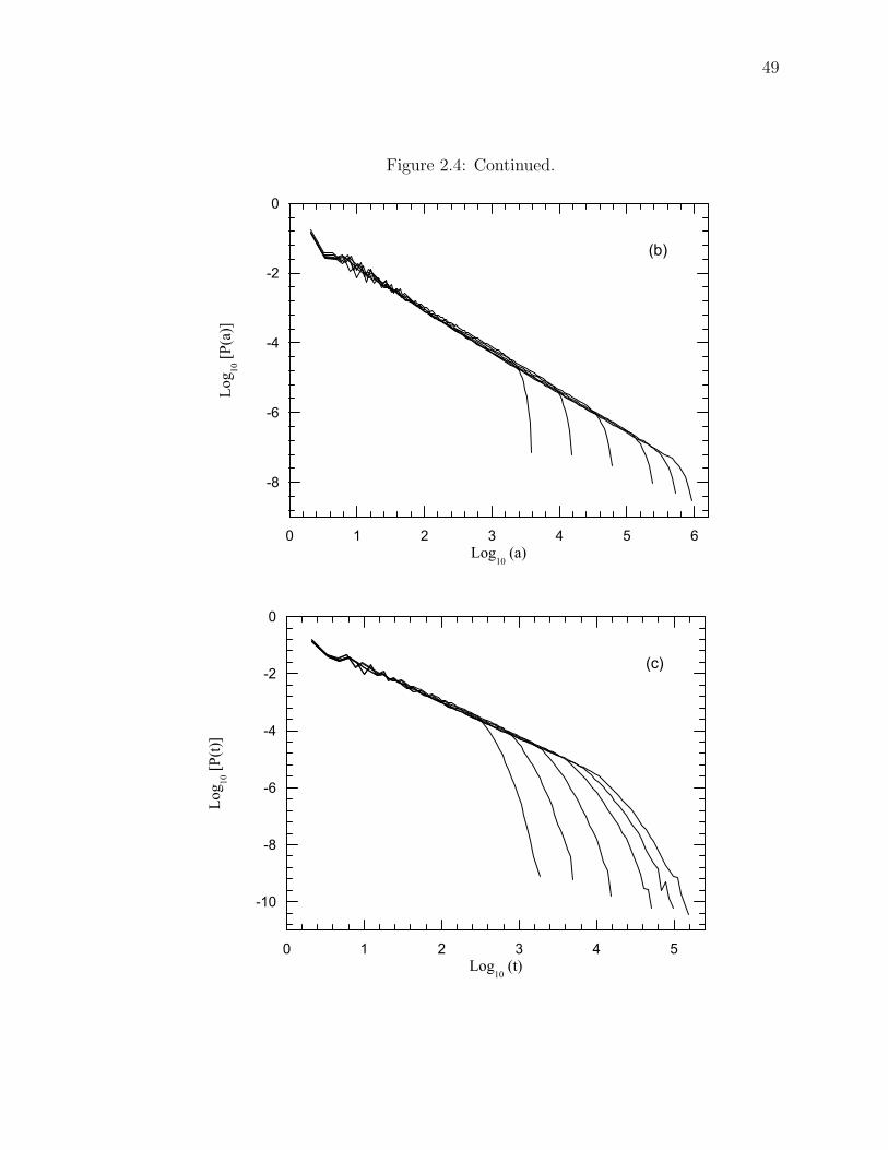
49

Figure 2.4: Continued.

0 1 2 3 4 5 6Log

10 (a)

-8

-6

-4

-2

0Lo

g 10 [P

(a)]

(b)

0 1 2 3 4 5Log

10 (t)

-10

-8

-6

-4

-2

0

Log 10

[P(t)

]

(c)

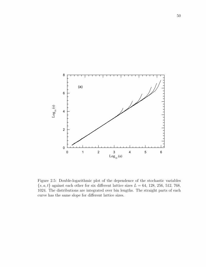
50

0 1 2 3 4 5 6Log

10 (a)

0

2

4

6

8

Log 10

(s)

(a)

Figure 2.5: Double-logarithmic plot of the dependence of the stochastic variabless, a, t against each other for six different lattice sizes L = 64, 128, 256, 512, 768,1024. The distributions are integrated over bin lengths. The straight parts of eachcurve has the same slope for different lattice sizes.

51

Figure 2.5: Continued.

0 1 2 3 4 5Log

10 (t)

0

2

4

6

8

Log 10

(s)

(b)

0 1 2 3 4 5Log

10 (t)

0

2

4

6

Log 10

(a)

(c)

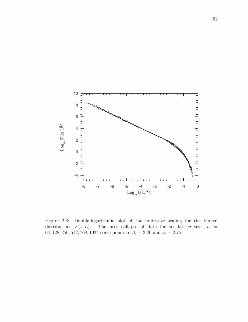
52

-8 -7 -6 -5 -4 -3 -2 -1 0Log

10 (s L−νs)

-4

-2

0

2

4

6

8

10

Log 10

[P(s

) Lβ s

]

Figure 2.6: Double-logarithmic plot of the finite-size scaling for the binneddistributions P (s, L). The best collapse of data for six lattice sizes L =64, 128, 256, 512, 768, 1024 corresponds to βs = 3.26 and νs = 2.75.

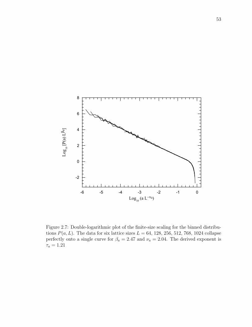
53

-6 -5 -4 -3 -2 -1 0Log

10 (a L−νa)

-2

0

2

4

6

8

Log 10

[P(a

) Lβ a

]

Figure 2.7: Double-logarithmic plot of the finite-size scaling for the binned distribu-tions P (a, L). The data for six lattice sizes L = 64, 128, 256, 512, 768, 1024 collapseperfectly onto a single curve for βa = 2.47 and νa = 2.04. The derived exponent isτa = 1.21

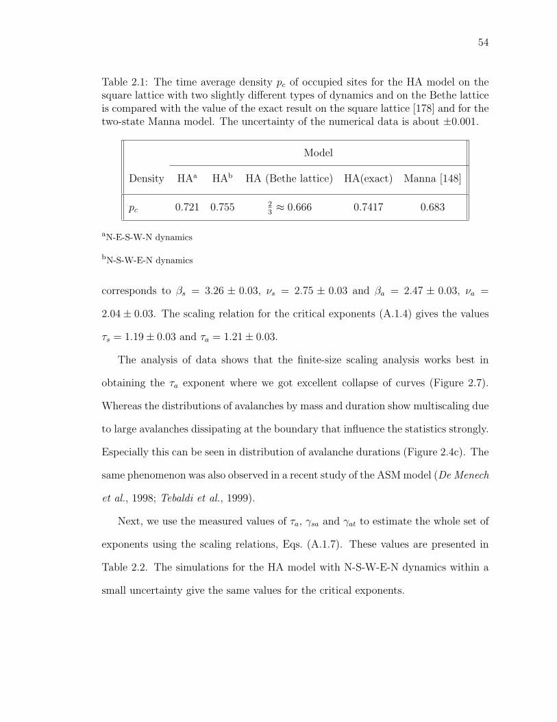
54

Table 2.1: The time average density pc of occupied sites for the HA model on thesquare lattice with two slightly different types of dynamics and on the Bethe latticeis compared with the value of the exact result on the square lattice [178] and for thetwo-state Manna model. The uncertainty of the numerical data is about ±0.001.

Model

Density HAa HAb HA (Bethe lattice) HA(exact) Manna [148]

pc 0.721 0.755 23≈ 0.666 0.7417 0.683

aN-E-S-W-N dynamics

bN-S-W-E-N dynamics

corresponds to βs = 3.26 ± 0.03, νs = 2.75 ± 0.03 and βa = 2.47 ± 0.03, νa =

2.04± 0.03. The scaling relation for the critical exponents (A.1.4) gives the values

τs = 1.19± 0.03 and τa = 1.21± 0.03.

The analysis of data shows that the finite-size scaling analysis works best in

obtaining the τa exponent where we got excellent collapse of curves (Figure 2.7).

Whereas the distributions of avalanches by mass and duration show multiscaling due

to large avalanches dissipating at the boundary that influence the statistics strongly.

Especially this can be seen in distribution of avalanche durations (Figure 2.4c). The

same phenomenon was also observed in a recent study of the ASM model (De Menech

et al., 1998; Tebaldi et al., 1999).

Next, we use the measured values of τa, γsa and γat to estimate the whole set of

exponents using the scaling relations, Eqs. (A.1.7). These values are presented in

Table 2.2. The simulations for the HA model with N-S-W-E-N dynamics within a

small uncertainty give the same values for the critical exponents.

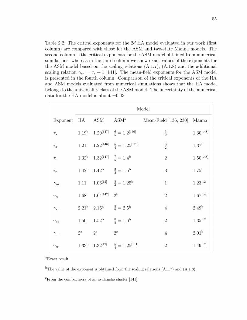
55

Table 2.2: The critical exponents for the 2d HA model evaluated in our work (firstcolumn) are compared with those for the ASM and two-state Manna models. Thesecond column is the critical exponents for the ASM model obtained from numericalsimulations, whereas in the third column we show exact values of the exponents forthe ASM model based on the scaling relations (A.1.7), (A.1.8) and the additionalscaling relation γsr = τr + 1 [141]. The mean-field exponents for the ASM modelis presented in the fourth column. Comparison of the critical exponents of the HAand ASM models evaluated from numerical simulations shows that the HA modelbelongs to the universality class of the ASM model. The uncertainty of the numericaldata for the HA model is about ±0.03.

Model

Exponent HA ASM ASMa Mean-Field [136, 230] Manna

τs 1.19b 1.20[147] 65

= 1.2[176] 32

1.30[148]

τa 1.21 1.22[146] 54

= 1.25[176] 32

1.37b

τt 1.32b 1.32[147] 75

= 1.4b 2 1.50[148]

τr 1.42b 1.42b 32

= 1.5b 3 1.75b

γsa 1.11 1.06[12] 54

= 1.25b 1 1.23[12]

γst 1.68 1.64[147] 2b 2 1.67[148]

γsr 2.21b 2.16b 52

= 2.5b 4 2.49b

γat 1.50 1.52b 85

= 1.6b 2 1.35[12]

γar 2c 2c 2c 4 2.01b

γtr 1.33b 1.32[12] 54

= 1.25[141] 2 1.49[12]

aExact result.

bThe value of the exponent is obtained from the scaling relations (A.1.7) and (A.1.8).

cFrom the compactness of an avalanche cluster [141].

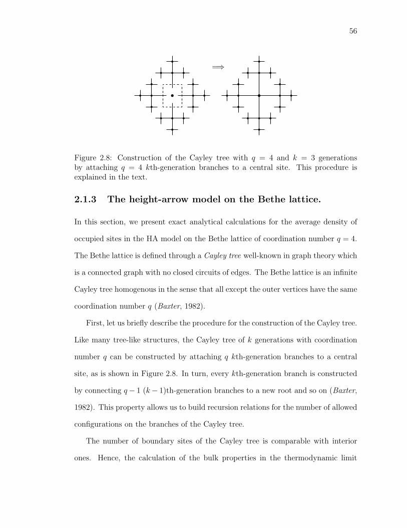
56

srrr r rr r rrr rrrr rr

=⇒

srrr r rr r rrr rrrr rr

Figure 2.8: Construction of the Cayley tree with q = 4 and k = 3 generationsby attaching q = 4 kth-generation branches to a central site. This procedure isexplained in the text.

2.1.3 The height-arrow model on the Bethe lattice.

In this section, we present exact analytical calculations for the average density of

occupied sites in the HA model on the Bethe lattice of coordination number q = 4.

The Bethe lattice is defined through a Cayley tree well-known in graph theory which

is a connected graph with no closed circuits of edges. The Bethe lattice is an infinite

Cayley tree homogenous in the sense that all except the outer vertices have the same

coordination number q (Baxter, 1982).

First, let us briefly describe the procedure for the construction of the Cayley tree.

Like many tree-like structures, the Cayley tree of k generations with coordination

number q can be constructed by attaching q kth-generation branches to a central

site, as is shown in Figure 2.8. In turn, every kth-generation branch is constructed

by connecting q− 1 (k− 1)th-generation branches to a new root and so on (Baxter,

1982). This property allows us to build recursion relations for the number of allowed

configurations on the branches of the Cayley tree.

The number of boundary sites of the Cayley tree is comparable with interior

ones. Hence, the calculation of the bulk properties in the thermodynamic limit

57

requires special care. Since we are interested in the solution on the Bethe lattice,

we will take the result for the average density of occupied sites calculated at the

central site of the Cayley tree as the value for the Bethe lattice.

The definition of the HA model on this connected graph with coordination num-

ber q = 4 remains unchanged. The only difference from the square lattice concerns

the notation of directions of arrows and sequences of their turns. Due to the 3-fold

permutation symmetry of branches growing from each site of the Bethe lattice the

calculation of various characteristics of the model does not depend on the sequences

of arrow turns.

Any configuration zi on the Cayley tree in which 1 ≤ zi ≤ q is a stable

configuration under the toppling rule. These configurations can be divided into two

classes: allowed and forbidden configurations (Dhar, 1990; Priezzhev, 1998). In the

SOC state, only allowed configurations have a nonzero probability.

Priezzhev (1998) defined a modified burning algorithm for the HA model to check

the type of stable configuration. It has been proven that to verify the type of a given

stable configuration C it is necessary to add q−qb particles at each boundary site of

the lattice, where q is a coordination number of the inner sites of the lattice and qb

is a coordination number of the boundary sites. If after addition of the particles we

obtain the initial configuration C then this configuration is an allowed configuration,

otherwise it is a forbidden one. In the case of the Cayley tree with q = 4 we add 3

particle at each boundary site to check the type of a stable configuration.

Following Dhar and Majumdar (1990), we approach the problem by dividing the

allowed configurations of the HA model in the SOC state into two types: strongly

allowed and weakly allowed and construct the recurrent relations for the ratio of

these configurations on the branches of the Bethe lattice. Using this ratio in the

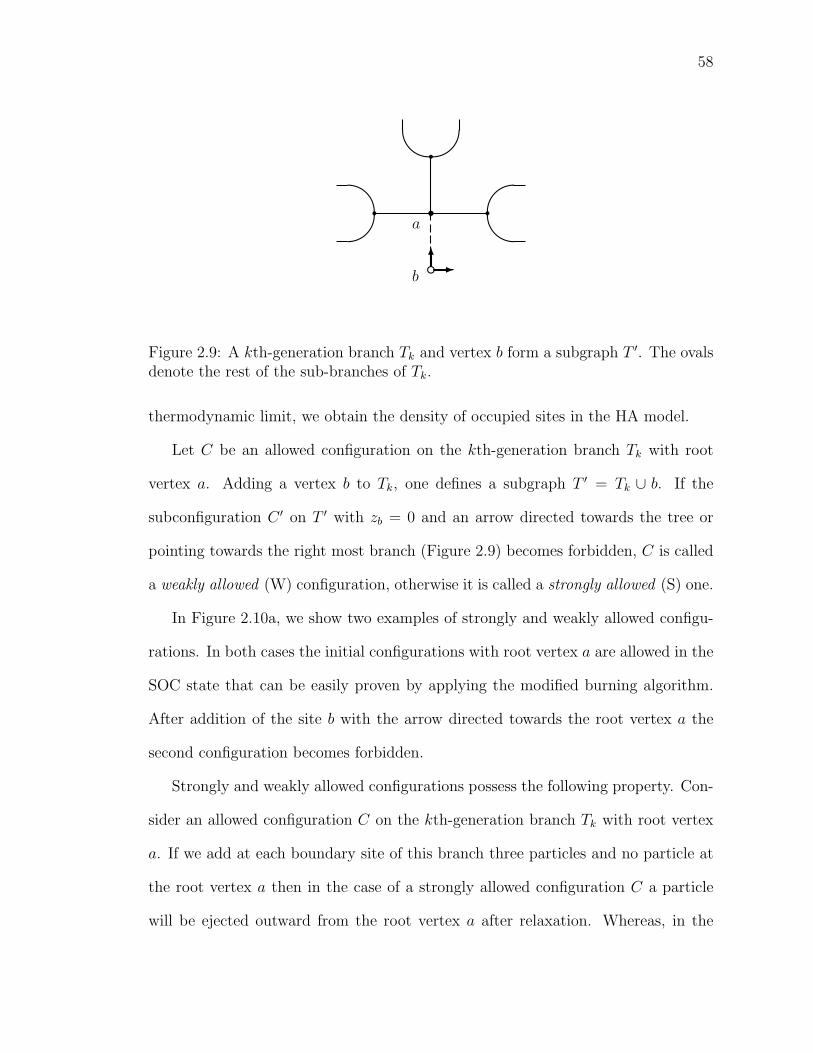
58

$%

& %'&

rr

rsa

db

6-

Figure 2.9: A kth-generation branch Tk and vertex b form a subgraph T ′. The ovalsdenote the rest of the sub-branches of Tk.

thermodynamic limit, we obtain the density of occupied sites in the HA model.

Let C be an allowed configuration on the kth-generation branch Tk with root

vertex a. Adding a vertex b to Tk, one defines a subgraph T ′ = Tk ∪ b. If the

subconfiguration C ′ on T ′ with zb = 0 and an arrow directed towards the tree or

pointing towards the right most branch (Figure 2.9) becomes forbidden, C is called

a weakly allowed (W) configuration, otherwise it is called a strongly allowed (S) one.

In Figure 2.10a, we show two examples of strongly and weakly allowed configu-

rations. In both cases the initial configurations with root vertex a are allowed in the

SOC state that can be easily proven by applying the modified burning algorithm.

After addition of the site b with the arrow directed towards the root vertex a the

second configuration becomes forbidden.

Strongly and weakly allowed configurations possess the following property. Con-

sider an allowed configuration C on the kth-generation branch Tk with root vertex

a. If we add at each boundary site of this branch three particles and no particle at

the root vertex a then in the case of a strongly allowed configuration C a particle

will be ejected outward from the root vertex a after relaxation. Whereas, in the

59

(I)

d

t -

t?

ta

-

db

6

(II)

t

t -

t?

da

db

6

Figure 2.10: Two examples of strongly and weakly allowed configurations. In bothcases the initial configurations (the tree without vertex b) are allowed. After additionof the vertex b and the arrow directed towards the root vertex a the configuration(I) remains allowed while the configuration (II) becomes forbidden. Therefore, theinitial allowed configuration in case (I) is strongly allowed and the initial allowedconfiguration in case (II) is weakly allowed.

case of a weakly allowed configuration C no particle will be ejected from the root

vertex a.

Now consider Tk with a root vertex a that consists of three (k− 1)th-generation

branches T(1)k−1, T

(2)k−1 and T

(3)k−1 with roots a1, a2 and a3, respectively (Figure 2.11).

Let NW (Tk, n, ↑) and NS(Tk, n, ↑) be the numbers of distinct W - and S-type con-

figurations on Tk with a given height za = n and direction of the arrow at the root

$%T

(1)k−1

a1

& %T(2)k−1

a2 '&T

(3)k−1

a3ss

ssa

Figure 2.11: A kth-generation branch Tk consists of three nearest (k − 1)th-

generation branches T(1)k−1, T

(2)k−1 and T

(3)k−1.

60

vertex a.

Let us also introduce

NW (Tk) =∑

n=0,1

∑r=↑,↓

NW (Tk, n, r) , (2.1.1)

NS(Tk) =∑

n=0,1

∑r=↑,↓

NS(Tk, n, r) , (2.1.2)

where the first summation is over the values of the heights and the second one is

over the directions of an arrow. As has been already mentioned, the arrow at each

site can take only two directions.

These numbers can be expressed in terms of the numbers of allowed subconfig-

urations on the three (k − 1)th-generation branches T(1)k−1, T

(2)k−1 and T

(3)k−1 (Papoyan

and Shcherbakov, 1995, 1996):

NW (Tk, 0, ↑) = 0 , (2.1.3)

NW (Tk, 0, ↓) = N(1)S N

(2)S N

(3)S +N

(1)S N

(2)W N

(3)S +N

(1)W N

(2)S N

(3)S +N

(1)W N

(2)W N

(3)S , (2.1.4)

NW (Tk, 1, ↓) = N(1)S N

(2)S N

(3)W +N

(1)S N

(2)W N

(3)W +N

(1)W N

(2)S N

(3)W , (2.1.5)

NW (Tk, 1, ↑) = N(1)W N

(2)W N

(3)W , (2.1.6)

NS(Tk, 0, ↑) = N(1)S N

(2)S N

(3)S +N

(1)S N

(2)S N

(3)W , (2.1.7)

NS(Tk, 0, ↓) = 0 , (2.1.8)

NS(Tk, 1, ↓) = N(1)S N

(2)S N

(3)S +N

(1)S N

(2)W N

(3)S +N

(1)W N

(2)S N

(3)S , (2.1.9)

NS(Tk, 1, ↑) = N(1)S N

(2)S N

(3)S +N

(1)S N

(2)S N

(3)W +N

(1)S N

(2)W N

(3)S +N

(1)S N

(2)W N

(3)W +

N(1)W N

(2)S N

(3)S +N

(1)W N

(2)S N

(3)W +N

(1)W N

(2)W N

(3)S , (2.1.10)

where N (i)α ≡ Nα(T

(i)k−1), α = W,S and i = 1, 2, 3. Adding (2.1.3)-(2.1.6) and

similarly (2.1.7)-(2.1.10) we get

NW (Tk) = N(1)S N

(2)S N

(3)S +N

(1)S N

(2)S N

(3)W +N

(1)S N

(2)W N

(3)S +N

(1)S N

(2)W N

(3)W +

61

N(1)W N

(2)S N

(3)S +N

(1)W N

(2)S N

(3)W +N

(1)W N

(2)W N

(3)S +N

(1)W N

(2)W N

(3)W , (2.1.11)

NS(Tk) = 3N(1)S N

(2)S N

(3)S +2N

(1)S N

(2)S N

(3)W +2N

(1)S N

(2)W N

(3)S +N

(1)S N

(2)W N

(3)W +

2N(1)W N

(2)S N

(3)S +N

(1)W N

(2)S N

(3)W +N

(1)W N

(2)W N

(3)S . (2.1.12)

Let us define

X =NW

NS

. (2.1.13)

If we consider graphs T(1)k−1, T

(2)k−1 and T

(3)k−1 to be isomorphic, then N(T

(1)k−1) =

N(T(2)k−1) = N(T

(3)k−1) and from (2.1.11) and (2.1.12) one obtains the following recur-

sion relation:

X(Tk) =1

3(1 +X(Tk−1)) . (2.1.14)

With the initial condition X(T0) = 13, this equation has a simple solution

X(Tk) =1

2− 1

23−(k+1) . (2.1.15)

In the thermodynamic limit (k →∞) the iterative sequence X(Tk) converges to a

stable point X∗ = 12

that characterizes the ratio of the weakly allowed configurations

to the strongly allowed ones in the SOC state.

Consider now a randomly chosen site O deep inside the Cayley tree (Figure 2.12).

The probability P (1) of occupation of the site O is

P (1) =N(1)

Ntotal

, (2.1.16)

where N(1) is the number of allowed configurations with z = 1 at the site O and

Ntotal = N(0) + N(1) is the total number of allowed configurations on the Cayley

tree. The numbers N(0) and N(1) can be expressed via the numbers of allowed

configurations on the four neighbor kth-generation branches T(i)k , i = 1, 2, 3, 4

N(0) = 2[1 + 2X +X2]4∏

i=1

NS(T (i)) , (2.1.17)

N(1) = 2[1 + 4X + 5X2 + 2X3]4∏

i=1

NS(T (i)) . (2.1.18)

62

$%T

(1)k

& %T(2)k

'&T

(3)k

' $T

(4)k

ss

ssjn

O-

Figure 2.12: A site O with height zo = n and a given direction of the arrow islocated deep inside the lattice and surrounded by the four kth-generation branchesT

(1)k , T

(2)k , T

(3)k and T

(4)k .

For the sites far from the surface in the thermodynamic limit (k → ∞) we have

X = 12. Thus, from( 2.1.17) and (2.1.18) we obtain

P (0) =1

3, P (1) =

2

3. (2.1.19)

The value for the concentration of occupied sites P (1) is in good qualitative agree-

ment with the numerical result obtained on the square lattice (Table 2.1).

2.1.4 The avalanche structure on the Bethe lattice.

Due to the absence of loops on the Bethe lattice the structure of an avalanche cluster

is simpler than on the square lattice. However, the presence of two variables at each

site of the lattice makes the calculation of the distribution of avalanches for any size

s rather difficult. We succeeded to calculate the distribution of avalanche sizes only

for the first several values of s, where the size s is the number of distinct toppled

sites in an avalanche.

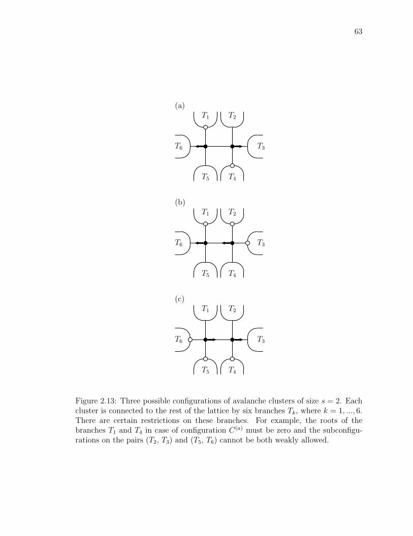
63

(a)

u u-

T1e T2

T3

T4

eT5

T6

(b)

u u

T1e T2e T3e

T4

T5

T6

(c)

u- u-

T1 T2

T3

T4

eT5

e

T6e

Figure 2.13: Three possible configurations of avalanche clusters of size s = 2. Eachcluster is connected to the rest of the lattice by six branches Tk, where k = 1, ..., 6.There are certain restrictions on these branches. For example, the roots of thebranches T1 and T4 in case of configuration C(a) must be zero and the subconfigu-rations on the pairs (T2, T3) and (T5, T6) cannot be both weakly allowed.

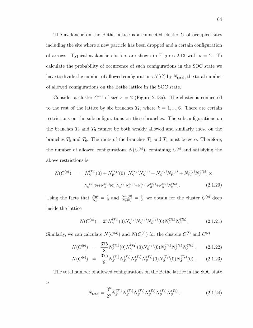
64

The avalanche on the Bethe lattice is a connected cluster C of occupied sites

including the site where a new particle has been dropped and a certain configuration

of arrows. Typical avalanche clusters are shown in Figures 2.13 with s = 2. To

calculate the probability of occurrence of such configurations in the SOC state we

have to divide the number of allowed configurationsN(C) byNtotal, the total number

of allowed configurations on the Bethe lattice in the SOC state.

Consider a cluster C(a) of size s = 2 (Figure 2.13a). The cluster is connected

to the rest of the lattice by six branches Tk, where k = 1, ..., 6. There are certain

restrictions on the subconfigurations on these branches. The subconfigurations on

the branches T2 and T3 cannot be both weakly allowed and similarly those on the

branches T5 and T6. The roots of the branches T1 and T4 must be zero. Therefore,

the number of allowed configurations N(C(a)), containing C(a) and satisfying the

above restrictions is

N(C(a)) = [N(T1)S (0) +N

(T1)W (0)][N

(T2)S N

(T3)S +N

(T2)S N

(T3)W +N

(T2)W N

(T3)S ]×

[N(T4)S (0)+N

(T4)W (0)][N

(T5)S N

(T6)S +N

(T5)S N

(T6)W +N

(T5)W N

(T6)S ] . (2.1.20)

Using the facts that NW

NS= 1

2and NW (0)

NS(0)= 3

2, we obtain for the cluster C(a) deep

inside the lattice

N(C(a)) = 25N(T1)S (0)N

(T2)S N

(T3)S N

(T4)S (0)N

(T5)S N

(T6)S . (2.1.21)

Similarly, we can calculate N(C(b)) and N(C(c)) for the clusters C(b) and C(c)

N(C(b)) =375

8N

(T1)S (0)N

(T2)S (0)N

(T3)S (0)N

(T4)S N

(T5)S N

(T6)S , (2.1.22)

N(C(c)) =375

8N

(T1)S N

(T2)S N

(T3)S N

(T4)S (0)N

(T5)S (0)N

(T6)S (0) . (2.1.23)

The total number of allowed configurations on the Bethe lattice in the SOC state

is

Ntotal =36

23N

(T1)S N

(T2)S N

(T3)S N

(T4)S N

(T5)S N

(T6)S , (2.1.24)

65

where we used the result (2.1.17) and (2.1.18) and the fact that the number of

strongly allowed configurations on some branch Tk can be expressed via the number

of strongly allowed configurations on the three adjacent sub-branches Tk−1 as

NS(Tk) =33

22NS(T

(1)k−1)NS(T

(2)k−1)NS(T

(3)k−1) .

Hence, we can obtain the probability of occurrence of avalanches of size s = 2

P (s = 2) =N(C(a)) + 1

2N(C(b)) + 1

2N(C(c))

Ntotal

, (2.1.25)

where the factor 12

in front of the terms N(C(b)) and N(C(c)) takes into account the

fact that only half of particles dropped on either of the two sites of the configurations

C(b) or C(c) start an avalanche.

Thus, using the result NS(0)NS

= 29, we finally get

P (s = 2) =3400

177147. (2.1.26)

We also calculated the probability of occurrence of avalanches of size s = 1

P (s = 1) = 2002187

. In principle, these probabilities can be derived for avalanches of

any finite size. We expect that for large s the distribution scales as P (s) ∼ s−3/2

which is a mean-field behavior for the distribution of avalanche sizes for the sandpile

model (Table 2.2).

2.2 Eulerian walkers model

2.2.1 Algebraic properties of the model

The Eulerian walkers model is defined as follows. Consider an arbitrary connected

graph G consisting of N sites. Each site of G is associated with an arrow which

is directed along one of the incident bonds. The arrow directions at the site i are

66

specified by the integers αi, (1 ≤ αi ≤ τi) where τi is the number of nearest neighbors

of the site i. The set αi gives a complete description of the medium. Starting

with an arbitrary arrow configuration one drops the particle to a site of G chosen

at random. At each time step:

i) the particle arriving at a site i changes the arrow direction from αi to αi + 1,

if αi < τi and to 1, if αi = τi

ii) the particle moves one step along the new arrow direction from i to the neigh-

boring site i′.

Having no endpoints on G, the particle continues to walk infinitely long. Due

to a finite number of possible states of the system, it eventually settles into the

Poincare cycle. For most dynamic systems the recurrence time of this cycle grows

exponentially with N . It has been shown (Priezzhev et al., 1996) that for the EWM

the Poincare cycle is squeezed to the Eulerian trail (Harary and Palmer, 1973) with

the recurrence time of an order of N . During the Eulerian trail the particle passes

all bonds of the graph exactly once in each direction.

There is the following simple interpretation of the dynamic rules of the model.

Let us consider a travelling merchant who buys and sells different kinds of goods

in towns connected by roads. All towns are supposed to produce different kinds of

goods. Upon arrival at a town, he sells all the goods bought in the previous town

and buys the new ones to be sold in a next town. Having bought some goods in

a town, say Dubna, the merchant goes to one of its nearest neighbors. Actually,

this town is not random. The merchant has a simple strategy to ensure the highest

level of sales revenues. First of all, if he never sold the goods produced in Dubna

in some of the neighboring towns, he chooses one of them (arbitrary) to visit next.

Then, if all the neighbors have already been visited, he prefers that neighbor where

67

he last sold the goods produced in Dubna earlier than at all the other neighbors.

If towns and roads connecting them are considered as sites and bonds of a graph,

respectively, then the merchant motion matches the rules of EWM dynamics.

Let G be an open graph. It means that one auxiliary site is introduced called a

sink. The subset of sites of G connected with the sink forms an open boundary. The

sink has no arrow and the particle reaching the sink leaves the system. Then, the

new particle is dropped to a site of G chosen at random. Since on the closed graph

the particle visits all sites during the walk, at the open graph it always reaches

the sink. A set C of configurations C = αj which remains on G when the

particle left G for the sink is the set of stable configurations. The operator ai can

be introduced as follows:

aiC = C ′ , (2.2.1)

which describes the resulting transformation by dropping the particle to the site

i. As usual in the theory of Markov chains, the set C may be divided into two

subsets. The first subset denoted by R includes those configurations which can

be obtained from an arbitrary configuration by a sequential action of the operators

ai. It follows from the definition that the subset R is closed under a multiple

action of the operators ai. Once the system gets into R, it never gets out under

subsequent evolution. All nonrecurrent configurations are called transient and form

the subset T which is the complement to the set R. By definition, any recurrent

configuration C ∈ R may be reached from another C ′ ∈ R by a subsequent

action of the operators ai. Since this is valid for C ′ = C too, the identity operator

acting in R exists. In addition, the operators ai have the following properties:

i) For arbitrary sites i and j and for any configuration of arrows C

ai aj C = aj aiC . (2.2.2)

68

ii) For any recurrent configuration C ∈ R, there exists a unique operator

(a−1i C) ∈ R

such that

ai (a−1i )C = C . (2.2.3)

The proof of these statements is similar to the one for the avalanche operators in

ASM (Dhar, 1990) and is given in (Priezzhev, 1994). Thus, the operators ai acting

in the set of recurrent configurations R form the Abelian group. The addition of

τi particles to site i gives the same effect as the addition of one particle to each of

τi neighbors of i. It returns the arrow outgoing from i to the former position and

initiates the motion of one particle to each neighboring site. In the operator form,

we have

aiτi =

τi∏k=1

ajk, (2.2.4)

where jk are neighbors of the site i. Introducing the discrete Laplacian on G as

∆ij =

τi , i = j

−1 , i and j are connected by a bond

0 , otherwise

(2.2.5)

and using Eq.(2.2.4), one can write the identity operator as

Ei =∏j∈G

a∆ij

j . (2.2.6)

Since all recurrent configurations can be obtained from an arbitrary one by a suc-

cessive action of operators ai, one can represent any C ∈ R in the form

C =∏i∈G

(ai)ni C∗. (2.2.7)

The N -dimensional vector n labels all possible recurrent configurations. Equation

(2.2.6) shows that two vectors n and n′ label the same configuration if the difference

69

between them is∑

j mj∆ij where mj are integers. The N -dimensional space n has

a periodic structure with an elementary cell of the form of a hyper-parallelepiped

with base edges ~ei = (∆i1,∆i2, ...,∆iN). Thus, the number of non-equivalent recur-

rent configurations is

N = det ∆ , (2.2.8)

which is the Kirchhoff formula (Harary and Palmer, 1973) for spanning trees and

the Dhar formula for the number of recurrent configurations in ASM (Dhar, 1990).

The correspondence to ASM is not surprising. The algebra of the operators ai

completely coincides with that of avalanche operators of the Abelian sandpile model

(Dhar, 1990). Moreover, the identity operator (2.2.6) has the same form for both

the models.

Continuing the analogy between recurrent configurations of EWM and sandpiles,

one can find the expected number Gij of full rotations of the arrow a site j, due to

the particle dropped at i (Dhar, 1990). During the walk, the expected number of

steps from j is ∆jjGij whereas −∑k 6=j Gik∆kj is the average flux into j. Equating

both the fluxes, one gets ∑k

Gik ∆kj = δij (2.2.9)

or

Gij = [∆−1]ij. (2.2.10)

The expected number of full rotations of the arrow is equal to the number of entries

into the site j divided by τj. On the other hand, the number of visits of a site

for the random walk is also the Green function of the Laplace equation. Thus, we

have a surprising fact that the number of visits of the site by the particle for the

deterministic motion in EWM coincides with that for the ordinary random walk.

70

The direct correspondence between spanning trees, recurrent configurations of

EWM and Eulerian trails can be established in the following way. The walking

particle leaves each site along an arrow after turning this arrow. Therefore, the

trajectory of the particle is traced by arrows. If G is an open graph, all trajectories

end at the sink and never form loops producing acyclic configurations of arrows.

Given an acyclic arrow configuration, we can construct a unique spanning tree

rooted in the sink and vice versa. Indeed, all bonds along which the arrows are

directed form the spanning tree. Conversely, if we have a spanning tree rooted

in the sink we can obtain the acyclic arrow configuration by pointing the arrow

from each site along the path leading to the sink. This correspondence allows us

to identify the acyclic arrow configurations and spanning trees. Below, we do not

distinguish between them and saying a spanning tree we mean both the spanning

tree and its arrow representation.

If G is the closed graph, the particle settles into the Eulerian trail during which it

passes each bond exactly once in each direction. Let the particle which has already

visited all sites, arrive at a site i at some moment. If we now remove the arrow from

i, we obtain the acyclic arrow configuration where all arrow paths lead to i. This

defines the spanning tree rooted in the site of the current particle location.

2.2.2 Avalanche dynamics

The particle added to the recurrent configuration of ASM may induce successive

topplings of sites called the avalanche. At the initial moment, it destroys the recur-

rent configuration and the system leaves the recurrent state. After the avalanche

stops, the recurrent configuration is restored again. Thus, the avalanche in ASM

can be defined as a period of reconstruction of the recurrent state. This definition

71

may be directly applied to EWM.

We start with a recurrent state of EWM. The corresponding arrow configuration

forms a spanning tree. Once a particle is dropped, it can destroy the spanning tree

by closing a loop of arrows. During the evolution, one loop can be transformed into

another. When all loops disappear, the spanning tree is restored. The interval of

existence of the loop can be called the avalanche of cyclicity or simply avalanche.

The loops can be created and destroyed several times during the motion of one

particle. Therefore, unlike ASM, an addition of one particle can initiate several

avalanches in the system. When a particle comes to the sink, it always directs the

arrows to the sink thus restoring the spanning tree. Therefore, when the particle

leaves the system, the avalanche always ends and the recurrent state is restored.

The particle dynamics represents successive transitions from one recurrent state to

another through avalanches. To study the evolution of the system, the structure of

the avalanche should be considered in detail.

Consider the Eulerian walk on the square lattice L of size L × L with open

boundary conditions. Each boundary site is connected to the sink by one bond on

the edge and by two bonds at the corners of L. The rule of arrow rotations is the

same for all sites. If we denote the bonds outgoing from a site i by N,E, S,W , the

rule of rotations is N → E → S → W . In other words, when the particle arrives

at a site, the arrow outgoing from this site turns to the next bond clockwise. For

a topological reason, this rule leads to a simple structure of avalanches, namely, to

clusters of sites visited by a particle, being compact.

Let the particle be dropped to a recurrent configuration which is a spanning

tree. At some step the first loop is created. The arrows can form loops of two

kinds: clockwise and anti-clockwise. The loop is clockwise if tracing the loop along

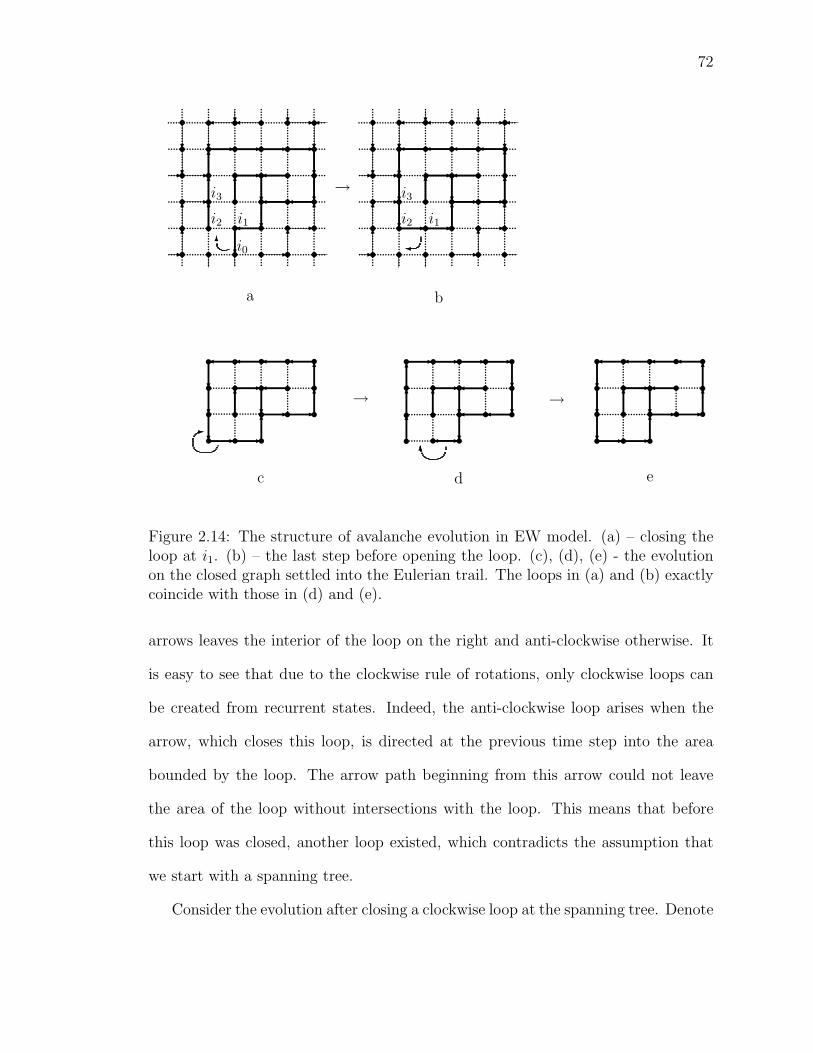
72

6 ?

?

?

?

----6

6

6

6?

-

-

?

?--

-6

6

?

? ?-

?

-6

-6

6?

-

- -6

-6

6

?

?

?

--

?

?--

-6

6

?

? ?-

?

-6

-6

?

?

?

----6

6

6

6?

-6

?

-

- -6

-6

6

?

?

?

-6

?

-

- -6

-6

6

?

?

?

-

s s s s ss ss s s s ss s s s s ss s s s s ss s s s s ss s s s s s

s s s s s ss s s s s ss s s s s ss s ss s ss s s s s ss s s s s s

-

s s s s ss s s s ss s s s ss s s -

6

s s s s ss s s s ss s s s ss s s

s s s s ss s s s ss s s s ss s s

→

→ →

............................................................

............................................................

............................................................

............................................................

............................................................

............................................................

....

....

....

....

....

....

....

..

....

....

..

....

....

....

....

....

....................

.......... ..........

..........

....................

..........

....

....

..

....

....

..

....

....

..

....

....

....

....

....

....................

.................... ..........

....

....

..

....

....

..

....

....

..

............................................................

............................................................

............................................................

............................................................

............................................................

............................................................

..........

....

....

..

............................................................

............................................................

............................................................

............................................................

............................................................

............................................................

............................................................

............................................................

............................................................

............................................................

............................................................

............................................................

a b

c d e

i2

i3

i1

i0

i3

i2 i1

Figure 2.14: The structure of avalanche evolution in EW model. (a) – closing theloop at i1. (b) – the last step before opening the loop. (c), (d), (e) - the evolutionon the closed graph settled into the Eulerian trail. The loops in (a) and (b) exactlycoincide with those in (d) and (e).

arrows leaves the interior of the loop on the right and anti-clockwise otherwise. It

is easy to see that due to the clockwise rule of rotations, only clockwise loops can

be created from recurrent states. Indeed, the anti-clockwise loop arises when the

arrow, which closes this loop, is directed at the previous time step into the area

bounded by the loop. The arrow path beginning from this arrow could not leave

the area of the loop without intersections with the loop. This means that before

this loop was closed, another loop existed, which contradicts the assumption that

we start with a spanning tree.

Consider the evolution after closing a clockwise loop at the spanning tree. Denote

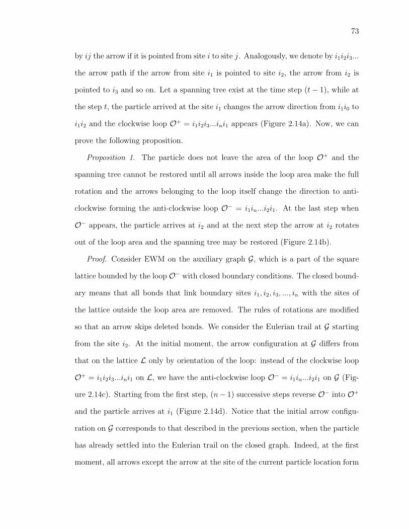
73

by ij the arrow if it is pointed from site i to site j. Analogously, we denote by i1i2i3...

the arrow path if the arrow from site i1 is pointed to site i2, the arrow from i2 is

pointed to i3 and so on. Let a spanning tree exist at the time step (t− 1), while at

the step t, the particle arrived at the site i1 changes the arrow direction from i1i0 to

i1i2 and the clockwise loop O+ = i1i2i3...ini1 appears (Figure 2.14a). Now, we can

prove the following proposition.

Proposition 1. The particle does not leave the area of the loop O+ and the

spanning tree cannot be restored until all arrows inside the loop area make the full

rotation and the arrows belonging to the loop itself change the direction to anti-

clockwise forming the anti-clockwise loop O− = i1in...i2i1. At the last step when

O− appears, the particle arrives at i2 and at the next step the arrow at i2 rotates

out of the loop area and the spanning tree may be restored (Figure 2.14b).

Proof. Consider EWM on the auxiliary graph G, which is a part of the square

lattice bounded by the loop O− with closed boundary conditions. The closed bound-

ary means that all bonds that link boundary sites i1, i2, i3, ..., in with the sites of

the lattice outside the loop area are removed. The rules of rotations are modified

so that an arrow skips deleted bonds. We consider the Eulerian trail at G starting

from the site i2. At the initial moment, the arrow configuration at G differs from

that on the lattice L only by orientation of the loop: instead of the clockwise loop

O+ = i1i2i3...ini1 on L, we have the anti-clockwise loop O− = i1in...i2i1 on G (Fig-

ure 2.14c). Starting from the first step, (n− 1) successive steps reverse O− into O+

and the particle arrives at i1 (Figure 2.14d). Notice that the initial arrow configu-

ration on G corresponds to that described in the previous section, when the particle

has already settled into the Eulerian trail on the closed graph. Indeed, at the first

moment, all arrows except the arrow at the site of the current particle location form

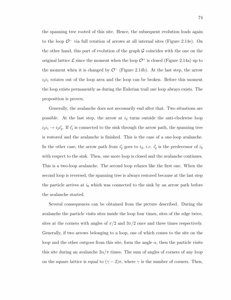
74

the spanning tree rooted of this site. Hence, the subsequent evolution leads again

to the loop O− via full rotation of arrows at all internal sites (Figure 2.14e). On

the other hand, this part of evolution of the graph G coincides with the one on the

original lattice L since the moment when the loop O+ is closed (Figure 2.14a) up to

the moment when it is changed by O− (Figure 2.14b). At the last step, the arrow

i2i1 rotates out of the loop area and the loop can be broken. Before this moment

the loop exists permanently as during the Eulerian trail one loop always exists. The

proposition is proven.

Generally, the avalanche does not necessarily end after that. Two situations are

possible. At the last step, the arrow at i2 turns outside the anti-clockwise loop

i2i1 → i2i′2. If i′1 is connected to the sink through the arrow path, the spanning tree

is restored and the avalanche is finished. This is the case of a one-loop avalanche.

In the other case, the arrow path from i′2 goes to i2, i.e. i′2 is the predecessor of i2

with respect to the sink. Then, one more loop is closed and the avalanche continues.

This is a two-loop avalanche. The second loop relaxes like the first one. When the

second loop is reversed, the spanning tree is always restored because at the last step

the particle arrives at i0 which was connected to the sink by an arrow path before

the avalanche started.

Several consequences can be obtained from the picture described. During the

avalanche the particle visits sites inside the loop four times, sites of the edge twice,

sites at the corners with angles of π/2 and 3π/2 once and three times respectively.

Generally, if two arrows belonging to a loop, one of which comes to the site on the

loop and the other outgoes from this site, form the angle α, then the particle visits

this site during an avalanche 2α/π times. The sum of angles of corners of any loop

on the square lattice is equal to (γ − 2)π, where γ is the number of corners. Then,

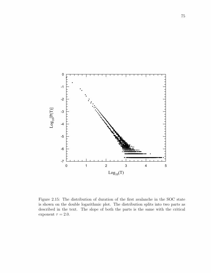
75

0 1 2 3 4 5

Log10(T)

-7

-6

-5

-4

-3

-2

-1

0

Log 10[P(T)]

Figure 2.15: The distribution of duration of the first avalanche in the SOC stateis shown on the double logarithmic plot. The distribution splits into two parts asdescribed in the text. The slope of both the parts is the same with the criticalexponent τ = 2.0.

76

the number of steps necessary to cover a loop is given by the formula

T = (4s+ 2(p− γ) + 2(γ − 2)) + 1 = (4s+ 2p− 4) + 1 , (2.2.11)

where s is the number of inner sites, and p is the perimeter of the loop. As the

avalanches can consist of one or two loops and the perimeter p is always even, the

duration of avalanches can be equal to any of the following numbers

T1 = 1 (mod 4) ,

T2 = 2 (mod 4) , (2.2.12)

where T1 and T2 are the durations of avalanches consisting of one and two loops,

respectively. This explains the double distribution of durations of avalanches (Fig-

ure 2.15) obtained in (Shcherbakov et al., 1997). Also we can find the critical ex-

ponent of the duration distribution for the first avalanche. In the thermodynamic

limit, the duration of avalanches grows as the area of the loop. It has been shown

(Manna et al., 1992) that the probability to get a loop of the size s when a bond is

added to the spanning tree at random is equal to

P (s) ∼ s−118 . (2.2.13)

In the distribution (2.2.13), the loop is assumed to be linked to the sink by unique

path attached to an arbitrary site its their perimeter, wherever it is closed by the

added bond. In our case, loops are closed by turning the arrow that was connected

to the sink through an arrow path before the turn. Hence, for the loop of perimeter

p, one should select only the latter case from p possible positions of the site linked

to the sink with respect to the place where the loop is closed. To this end, the

distribution (2.2.13) should be divided by the perimeter of the loop. Taking into

account that the perimeter p of the loop scales with the linear size r as the fractal

77

dimension of a chemical path on a spanning tree (Manna et al., 1992) p ∼ r54 and

that the loop is compact s ∼ r2, we obtain

P(s) ∼ s−118

r54

∼ s−2 . (2.2.14)

Thus, for the first avalanches the critical exponent of the distribution of duration

is τ = 2. The one- and two-loop avalanches differ only in a local structure of

the spanning tree at the site of closing the loop. Therefore, the critical exponents

are the same for both the distributions. This result is in excellent agreement with

numerical simulations presented in Figure 2.15 where we have considered the EWM

on the square lattice of linear size L = 400 with open boundary conditions.

The first avalanche in EWM are similar to the erased loops in the loop-erased

walks, studied by Dhar and Dhar, (1997). The same exponent τ = 2 was obtained.

The result τ = 2 is valid only for the first avalanches for their independence of

each other. The analytic derivation of τ for arbitrary avalanches is a more difficult

problem due to correlations between subsequent avalanches appearing during the

motion of one particle.

2.2.3 Numerical simulations

To investigate the avalanche process in the models of self-organizing Eulerian walk-

ers, we studied them numerically with high statistics. For each distribution of

avalanches we considered up to 30 · 106 events on the square lattices of linear size L

from 120 to 400. Simulations always started from the regular initial configuration

in which all arrows were directed up.

In Figure2.16, we present the double logarithmic plot of the distribution P (s)

of the number of visited sites in the avalanche for the lattice size L = 400. The

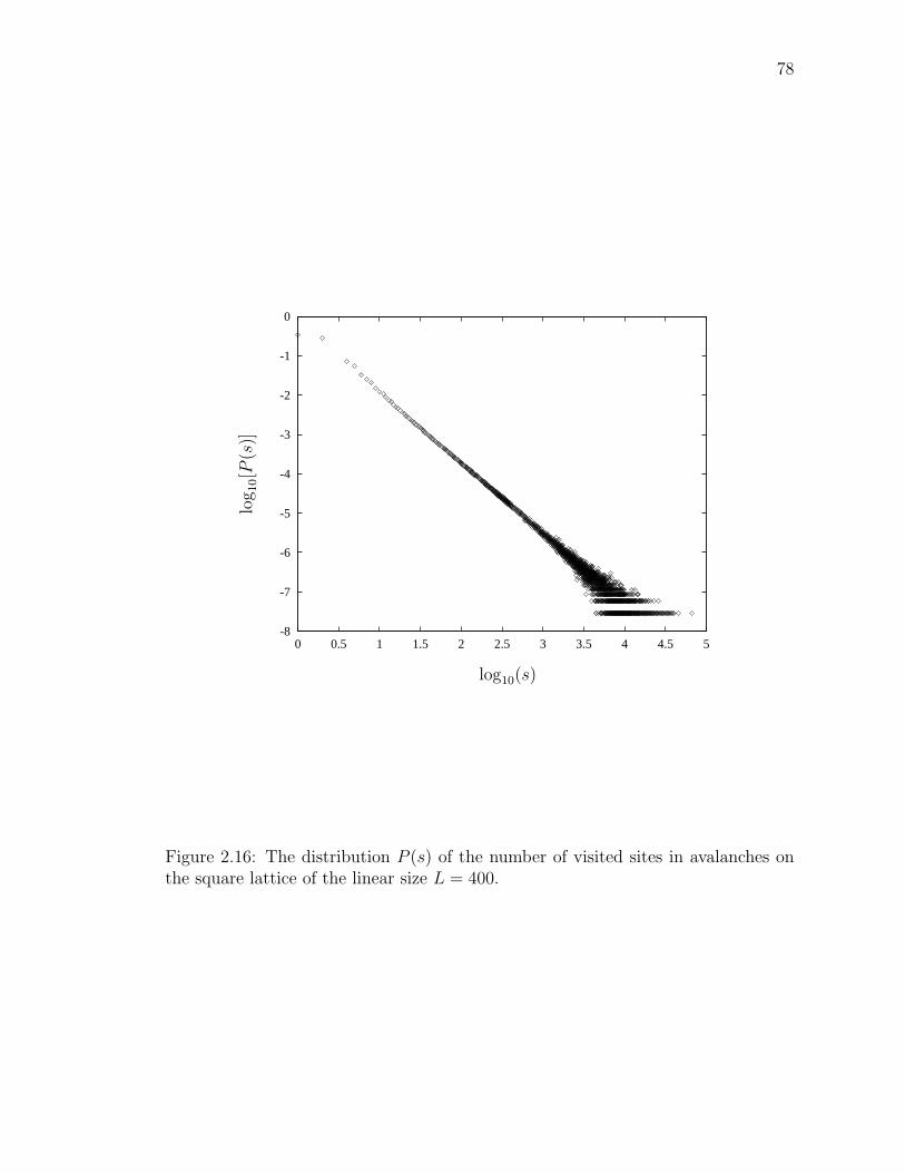
78

-8

-7

-6

-5

-4

-3

-2

-1

0

0 0.5 1 1.5 2 2.5 3 3.5 4 4.5 5

log10(s)

log

10[P

(s)]

Figure 2.16: The distribution P (s) of the number of visited sites in avalanches onthe square lattice of the linear size L = 400.

79

analysis of the data shows that this distribution obeys the power law

P (s) ∼ s−τs . (2.2.15)

To estimate the critical exponents, we have performed the finite-size scaling

analysis (see Appendix A) assuming the distribution functions scale with the lattice

size L as

P (x, L) = L−βf(x/Lν) , (2.2.16)

where f(y) is a universal scaling function and β and ν are critical exponents which

describe the scaling of the distribution function.

To reduce the fluctuations of the data, we integrated each distribution over

exponentially increasing bin lengths. For the integrated bin distribution we have

(Manna, 1991)

D(s) =∫P (x) dx ∼ s−(τs−1) . (2.2.17)

Plotting D(s, L)Lβs versus sL−νs on a double logarithmic scale, as is shown in

Figure 2.17 for the different lattice sizes L, we obtained that the best data collapse

corresponds to βs = 1.5 ± 0.05, νs = 2.0 ± 0.05 (Figure 2.18). The scaling relation

for the critical exponents τs = βs/νs + 1 gives the value τs = 1.75± 0.05.

In the same way, we investigated the distribution P (l) of the number of steps

performed by the particle in the avalanche for the different lattice sizes L. There is

an explicit power law behavior in these distributions (Figure 2.19)

P (l) ∼ l−τl (2.2.18)

with the finite size cutoff. We applied the finite-size scaling analysis to the integrated

distributions and obtained τl = 1.7± 0.05 from the best data collapse.

We also investigated a slightly modified model. The difference from the previous

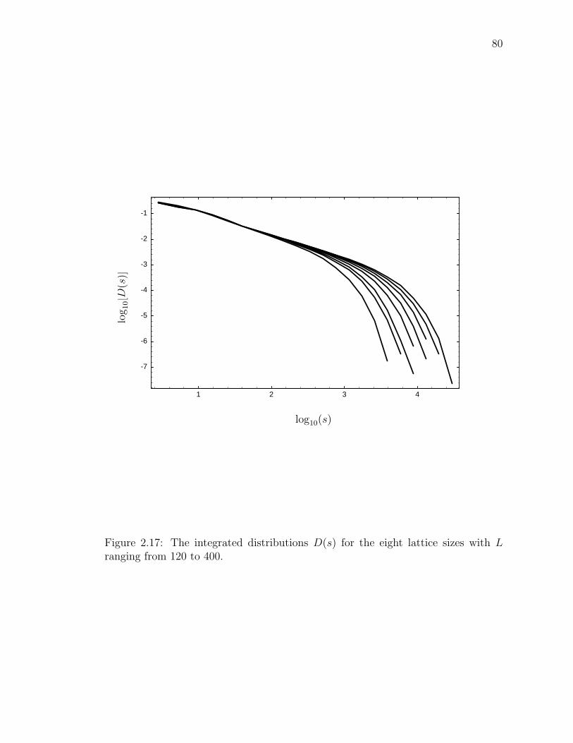
80

1 2 3 4

-7

-6

-5

-4

-3

-2

-1

log10(s)

log

10[D

(s)]

Figure 2.17: The integrated distributions D(s) for the eight lattice sizes with Lranging from 120 to 400.

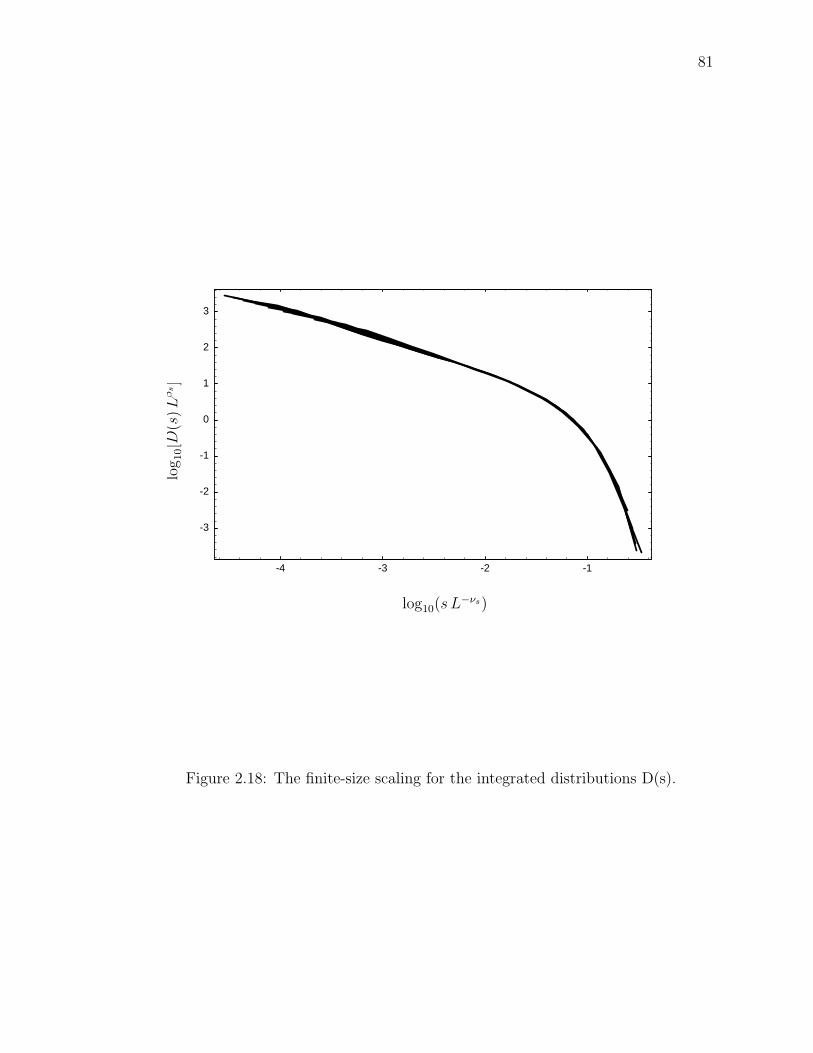
81

-4 -3 -2 -1

-3

-2

-1

0

1

2

3

log10(s L−νs)

log

10[D

(s)L

βs]

Figure 2.18: The finite-size scaling for the integrated distributions D(s).

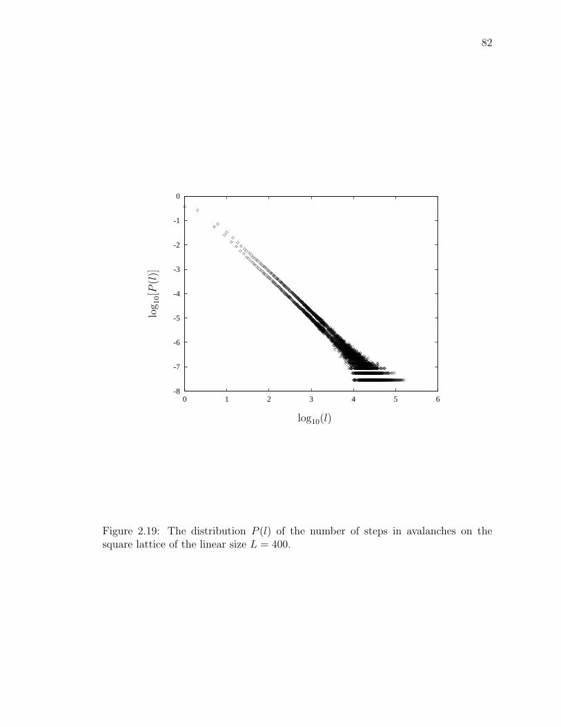
82

-8

-7

-6

-5

-4

-3

-2

-1

0

0 1 2 3 4 5 6

log10(l)

log

10[P

(l)]

Figure 2.19: The distribution P (l) of the number of steps in avalanches on thesquare lattice of the linear size L = 400.

83

one is in the order of turns of the arrow. In the case when the turns form the sequence

(up-down-left-right-up), we found a similar power law for avalanche distributions.

To find critical exponents of this power law from finite-size scaling analysis, we

integrated again these distributions over exponentially increasing bin lengths. The

critical exponents τl = 1.72± 0.05 and τs = 1.8± 0.05 have been obtained from the

best data collapse for the distribution of steps and visited sites, respectively.

2.2.4 Diffusion of Eulerian walkers

Besides the evolution of the system as a whole, we can describe the motion of a

particle itself. Consider the particle dropped on the lattice with a spanning tree.

We call the site i a predecessor of j if the arrow path comes from i to j. Since the

particle trajectory is traced by arrows, all visited sites are predecessors of the site of

a current particle location. If the particle arrives at the site which is its predecessor,

the loop is closed. Thus, the particle can visit the sites that have already been

visited only during an avalanche.

We divide the motion of the particle into the following stages. The first stage

coincides with the first avalanche. At the moment it finishes, the avalanche area

remains bounded by the anti-clockwise loop opened at the bond connecting two sites

where the avalanche begins and where it ends. Further, moving on the lattice, the

particle cannot enter the area of the first avalanche until it creates a loop enclosing

this area. For this time, new avalanches appear beyond the first one being attached

to its boundary and tending to go clockwise around it. Eventually, the particle

creates a loop enclosing the area of the first avalanche and visits it again. When the

avalanche corresponding to this loop ends, the second stage of the evolution finishes.

At this moment, we have the cluster of visited sites which consists of the area of

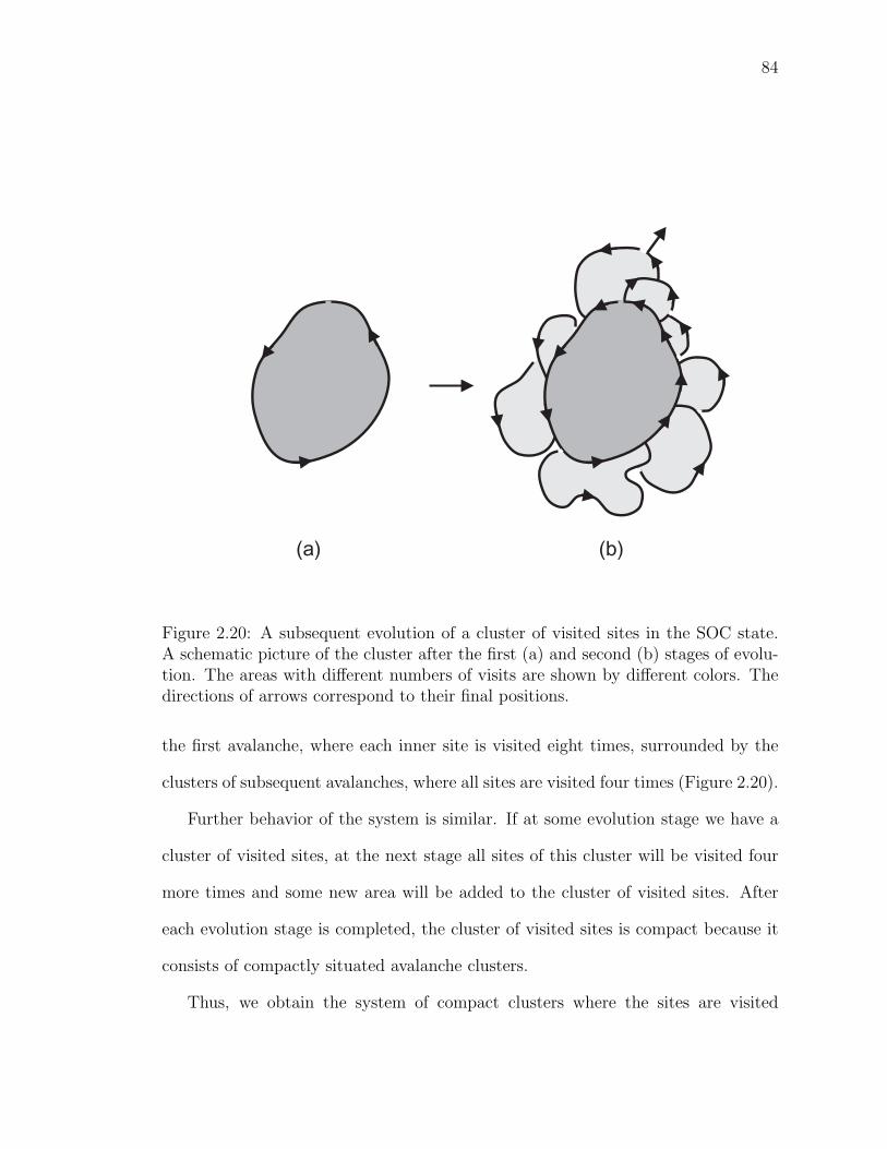
84

(b)(a)

Figure 2.20: A subsequent evolution of a cluster of visited sites in the SOC state.A schematic picture of the cluster after the first (a) and second (b) stages of evolu-tion. The areas with different numbers of visits are shown by different colors. Thedirections of arrows correspond to their final positions.

the first avalanche, where each inner site is visited eight times, surrounded by the

clusters of subsequent avalanches, where all sites are visited four times (Figure 2.20).

Further behavior of the system is similar. If at some evolution stage we have a

cluster of visited sites, at the next stage all sites of this cluster will be visited four

more times and some new area will be added to the cluster of visited sites. After

each evolution stage is completed, the cluster of visited sites is compact because it

consists of compactly situated avalanche clusters.

Thus, we obtain the system of compact clusters where the sites are visited

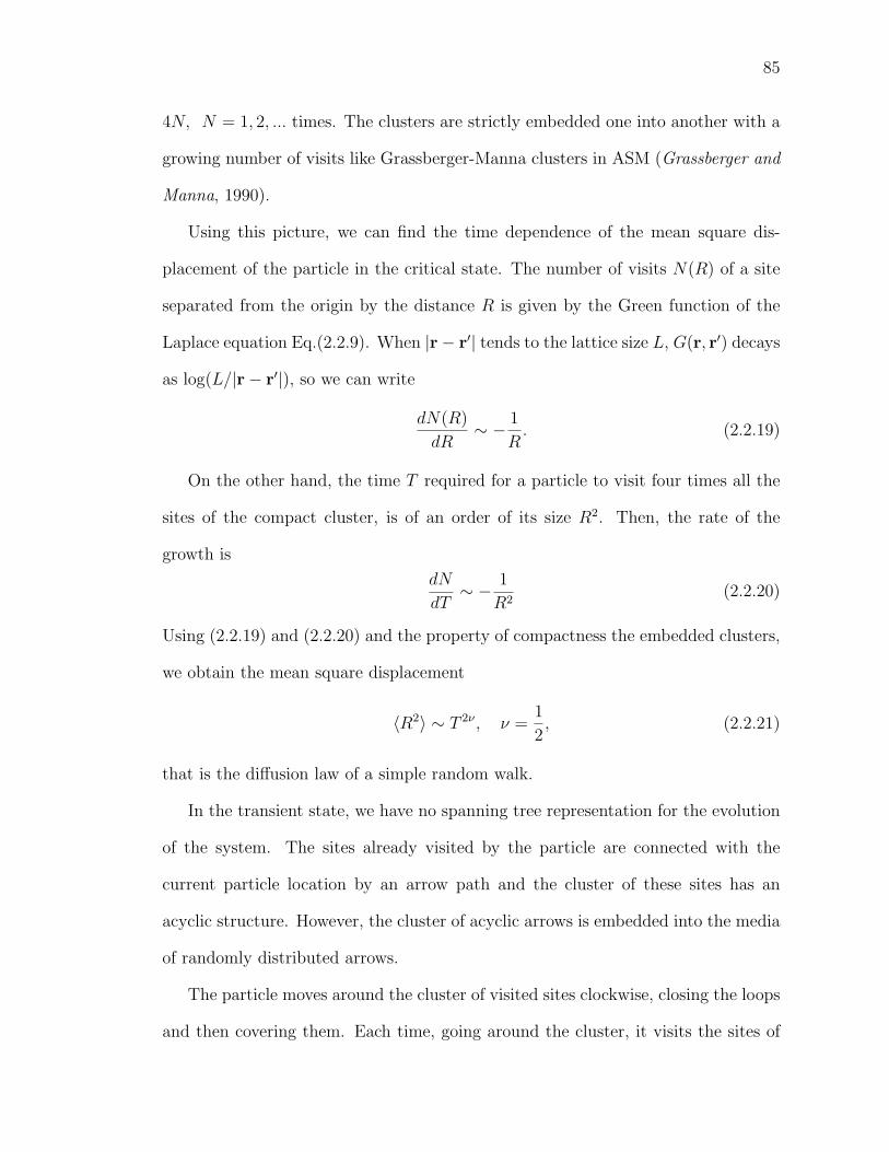
85

4N, N = 1, 2, ... times. The clusters are strictly embedded one into another with a

growing number of visits like Grassberger-Manna clusters in ASM (Grassberger and

Manna, 1990).

Using this picture, we can find the time dependence of the mean square dis-

placement of the particle in the critical state. The number of visits N(R) of a site

separated from the origin by the distance R is given by the Green function of the

Laplace equation Eq.(2.2.9). When |r− r′| tends to the lattice size L, G(r, r′) decays

as log(L/|r− r′|), so we can write

dN(R)

dR∼ − 1

R. (2.2.19)

On the other hand, the time T required for a particle to visit four times all the

sites of the compact cluster, is of an order of its size R2. Then, the rate of the

growth is

dN

dT∼ − 1

R2(2.2.20)

Using (2.2.19) and (2.2.20) and the property of compactness the embedded clusters,

we obtain the mean square displacement

〈R2〉 ∼ T 2ν , ν =1

2, (2.2.21)

that is the diffusion law of a simple random walk.

In the transient state, we have no spanning tree representation for the evolution

of the system. The sites already visited by the particle are connected with the

current particle location by an arrow path and the cluster of these sites has an

acyclic structure. However, the cluster of acyclic arrows is embedded into the media

of randomly distributed arrows.

The particle moves around the cluster of visited sites clockwise, closing the loops

and then covering them. Each time, going around the cluster, it visits the sites of

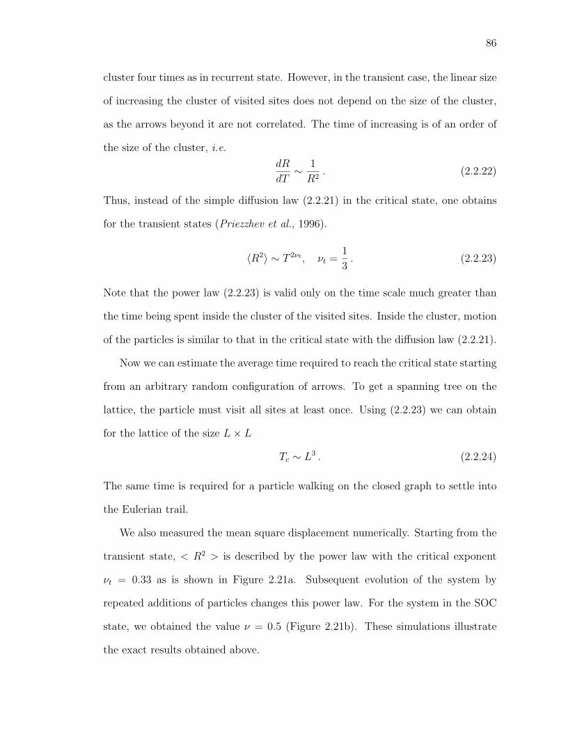
86

cluster four times as in recurrent state. However, in the transient case, the linear size

of increasing the cluster of visited sites does not depend on the size of the cluster,

as the arrows beyond it are not correlated. The time of increasing is of an order of

the size of the cluster, i.e.

dR

dT∼ 1

R2. (2.2.22)

Thus, instead of the simple diffusion law (2.2.21) in the critical state, one obtains

for the transient states (Priezzhev et al., 1996).

〈R2〉 ∼ T 2νt , νt =1

3. (2.2.23)

Note that the power law (2.2.23) is valid only on the time scale much greater than

the time being spent inside the cluster of the visited sites. Inside the cluster, motion

of the particles is similar to that in the critical state with the diffusion law (2.2.21).

Now we can estimate the average time required to reach the critical state starting

from an arbitrary random configuration of arrows. To get a spanning tree on the

lattice, the particle must visit all sites at least once. Using (2.2.23) we can obtain

for the lattice of the size L× L

Tc ∼ L3 . (2.2.24)

The same time is required for a particle walking on the closed graph to settle into

the Eulerian trail.

We also measured the mean square displacement numerically. Starting from the

transient state, < R2 > is described by the power law with the critical exponent

νt = 0.33 as is shown in Figure 2.21a. Subsequent evolution of the system by

repeated additions of particles changes this power law. For the system in the SOC

state, we obtained the value ν = 0.5 (Figure 2.21b). These simulations illustrate

the exact results obtained above.

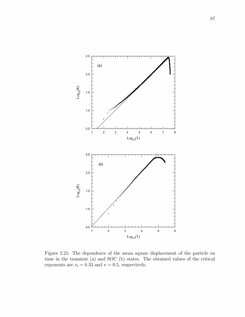
87

1 2 3 4 5 6 7 8

Log10(T)

0.5

1.0

1.5

2.0

2.5

Log 10(R)

(a)

1 2 3 4 5 6

Log10(T)

0.5

1.0

1.5

2.0

2.5

Log 10(R)

(b)

Figure 2.21: The dependence of the mean square displacement of the particle ontime in the transient (a) and SOC (b) states. The obtained values of the criticalexponents are νt = 0.33 and ν = 0.5, respectively.

88

In summary, we considered the dynamics of the Eulerian Walkers Model. The

structure of avalanches in the SOC state was studied in detail. We obtained the

critical exponent for the distribution of durations of the first avalanche. Considering

the evolution of the system as a sequence of avalanches, we found the simple diffu-

sion law for the mean square displacement of the particle in the SOC state. The

crossover from the transient state into the SOC state was described qualitatively.

The obtained exact results were confirmed by numerical simulations.

Chapter 3

Earthquakes and Damage

Mechanics

3.1 Micro- and macro-scopic models of fracture

and damage

3.1.1 Introduction

In this section we will consider both microscopic and continuum models of damage.

We will compare both types of models with laboratory experiments and will discuss

the implications for earthquake physics. The behavior of a rod of material under

tension is illustrated schematically in Figure 3.1. Deviations from linear elasticity

and the existence of damage are shown schematically. The stress σ in the rod is

given as a function of the strain ε. In region I, linear elasticity is applicable and we

have

σ = E0 ε , (3.1.1)

89

90

where E0 is the Young’s modulus of the undamaged material, a constant. In region

II, where there is a deviation from linear elasticity, microcracking is occurring. These

microcracks weaken the material and result in acoustic emissions. For a prescribed

stress σ, the strain ε is greater than the value given by (3.1.1). Accordingly, we

write

σ = Eeff ε (3.1.2)

where Eeff is the effective Young’s modulus—it is no longer assumed to be a constant.

This relation between σ and ε provides the definition of Eeff .

A continuum approach to this process is to introduce a damage variable α so

that (Kachanov, 1986; Lemaitre and Chaboche, 1990; Lyakhovsky et al., 1993; Kra-

jcinovic, 1996; Lyakhovsky et al., 1997)

Eeff = E0 (1− α) . (3.1.3)

The damage variable α quantifies the deviation from linear elasticity and the dis-

tribution of microcracks in the one-dimensional problem. In general 0 ≤ α ≤ 1.

With α = 0, linear elasticity is obtained with (3.1.1) valid, but when α = 1, failure

occurs. For quasistatic (slow) rupture it is appropriate to take the damage variable

to be a function only of the applied stress α(σ). However, in most cases of interest

the development of damage in a material is a transient process so that we have

α [σ (t) , t]. As illustrated in Figure 3.1, the failure of the brittle material occurs

when σ(tf ) = σf (α = 1), the failure stress. It should be emphasized that the

dependence given in Figure 3.1 is highly idealized since the dependence on time is

not illustrated.

Based upon thermodynamic considerations (Kachanov, 1986; Krajcinovic, 1996;

Lyakhovsky et al., 1997), the time evolution of the damage variable is related to the

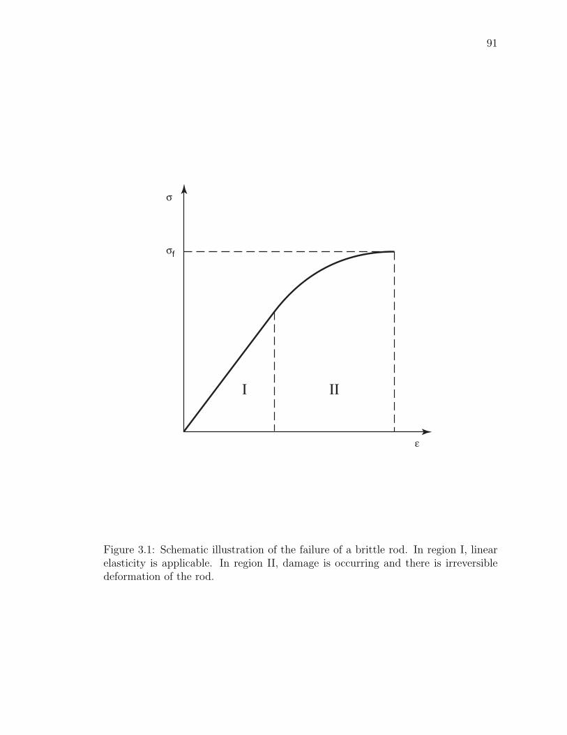
91

σ

σf

ε

Ι ΙΙ

Figure 3.1: Schematic illustration of the failure of a brittle rod. In region I, linearelasticity is applicable. In region II, damage is occurring and there is irreversibledeformation of the rod.

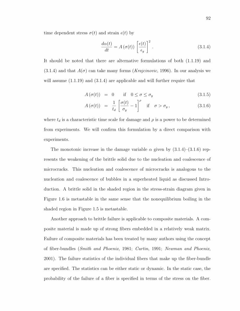
92

time dependent stress σ(t) and strain ε(t) by

dα(t)

dt= A (σ(t))

[ε(t)

εy

]2

. (3.1.4)

It should be noted that there are alternative formulations of both (1.1.19) and

(3.1.4) and that A(σ) can take many forms (Krajcinovic, 1996). In our analysis we

will assume (1.1.19) and (3.1.4) are applicable and will further require that

A (σ(t)) = 0 if 0 ≤ σ ≤ σy (3.1.5)

A (σ(t)) =1

td

[σ(t)

σy

− 1

]ρ

if σ > σy , (3.1.6)

where td is a characteristic time scale for damage and ρ is a power to be determined

from experiments. We will confirm this formulation by a direct comparison with

experiments.

The monotonic increase in the damage variable α given by (3.1.4)–(3.1.6) rep-

resents the weakening of the brittle solid due to the nucleation and coalescence of

microcracks. This nucleation and coalescence of microcracks is analogous to the

nucleation and coalescence of bubbles in a superheated liquid as discussed Intro-

duction. A brittle solid in the shaded region in the stress-strain diagram given in

Figure 1.6 is metastable in the same sense that the nonequilibrium boiling in the

shaded region in Figure 1.5 is metastable.

Another approach to brittle failure is applicable to composite materials. A com-

posite material is made up of strong fibers embedded in a relatively weak matrix.

Failure of composite materials has been treated by many authors using the concept

of fiber-bundles (Smith and Phoenix, 1981; Curtin, 1991; Newman and Phoenix,

2001). The failure statistics of the individual fibers that make up the fiber-bundle

are specified. The statistics can be either static or dynamic. In the static case, the

probability of the failure of a fiber is specified in terms of the stress on the fiber.

93

Failure is assumed to occur instantaneously. In the dynamic case, the statistical

distribution of times to failure for the fibers are specified in terms of the stresses on

the fibers (Coleman, 1956, 1958). Experiments generally favor the dynamic-failure,

fiber-bundle models. When stress is applied to a fiber-bundle, the fibers begin to

fail. It is necessary to specify how the stress on a failed fiber is redistributed to

the remaining sound fibers (Smith and Phoenix, 1981). In the uniform load sharing

hypothesis, the stress from a failed fiber is redistributed equally to the remaining

fibers. This is a mean-field approximation. The alternative redistribution model is

the local load sharing hypothesis. In this case the load on the failed fiber is redis-

tributed to neighboring fibers. Local load sharing is applicable to strongly bonded

fibrous (composite) materials whereas equal load sharing is applicable to weakly

bonded fibrous materials.

The failure of a simple fiber-bundle under uniform load sharing is illustrated in

Figure 3.2. Initially the load on the bundle F0 is carried equally by the four fibers

with F = 14F0. The weakest fiber fails and the load on that fiber is now carried

by the surviving fibers with F = 13F0. The stress on each fiber increases from

the original value σ0 to 43σ0. The process of failure followed by stress redistribution

continues until all fibers fail and no load can be carried. The fiber-bundle model can

also be used as a simple model for friction where the fibers represent the asperities

on a surface.

3.1.2 Fiber-bundle model

We consider a rod that is made up of N0 fibers. This rod can be thought of as a

frictionless, stranded cable made up of N0 strands. The standard approach to the

dynamic time dependent failure of a fiber-bundle is to specify an expression for the

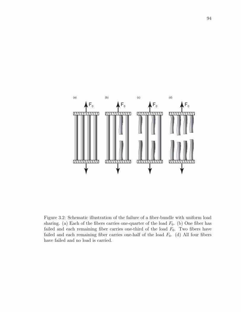
94

F0 F0 F0 F0

(a) (b) (c) (d)

Figure 3.2: Schematic illustration of the failure of a fiber-bundle with uniform loadsharing. (a) Each of the fibers carries one-quarter of the load F0. (b) One fiber hasfailed and each remaining fiber carries one-third of the load F0. Two fibers havefailed and each remaining fiber carries one-half of the load F0. (d) All four fibershave failed and no load is carried.

95

rate of failure of fibers (Coleman, 1956, 1958; Newman and Phoenix, 2001). The

form of this breakdown rule is given by

d

dt[N0 −Nf (t)] = −ν(σ) [N0 −Nf (t)] , (3.1.7)

where Nf (t) is the cumulative number of fibers that have failed at time t, N0−Nf (t)

is thus the number of unbroken fibers, and ν(σ) is known as the hazard rate, which

is a function of the applied stress σ(t).

We first consider the case in which a uniform strain ε0 is applied to the fiber-

bundle at time t = 0. In this case the stress on each fiber has a constant value σ0

given by (3.1.1), where E0 is the Young’s modulus of a fiber. Since the stress on the

fibers is constant, so is the hazard rate, yielding ν = ν0 independent of time t. In

this case (3.1.7) can be integrated to give

N0 −Nf (t)

N0

= e−ν0 t , (3.1.8)

where the initial conditions Nf (0) = 0 has been used. The cumulative distribution

function pc(t) that a fiber has failed at time t is given by

pc(t) =Nf (t)

N0

= 1− e−ν0 t . (3.1.9)

The total force F (t) carried by the fiber-bundle at the time t is given by

F (t) = [N0 −Nf (t)] σ0 a , (3.1.10)

where a is the area of a fiber. Substituting (3.1.1) and (3.1.8) into (3.1.10) gives

F (t) = N0 aE0 ε e−ν0 t . (3.1.11)

The force on the fiber-bundle decreases as fibers fail and catastrophic failure in a

finite time does not occur.

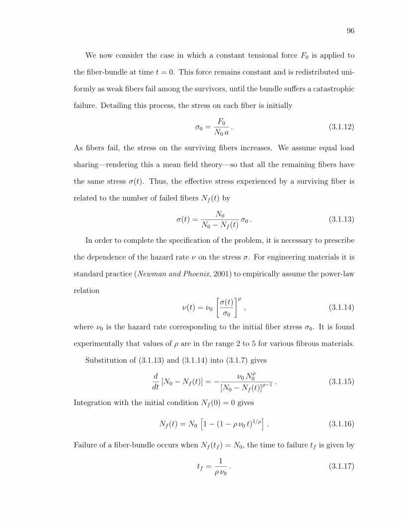
96

We now consider the case in which a constant tensional force F0 is applied to

the fiber-bundle at time t = 0. This force remains constant and is redistributed uni-

formly as weak fibers fail among the survivors, until the bundle suffers a catastrophic

failure. Detailing this process, the stress on each fiber is initially

σ0 =F0

N0 a. (3.1.12)

As fibers fail, the stress on the surviving fibers increases. We assume equal load

sharing—rendering this a mean field theory—so that all the remaining fibers have

the same stress σ(t). Thus, the effective stress experienced by a surviving fiber is

related to the number of failed fibers Nf (t) by

σ(t) =N0

N0 −Nf (t)σ0 . (3.1.13)

In order to complete the specification of the problem, it is necessary to prescribe

the dependence of the hazard rate ν on the stress σ. For engineering materials it is

standard practice (Newman and Phoenix, 2001) to empirically assume the power-law

relation

ν(t) = ν0

[σ(t)

σ0

]ρ

, (3.1.14)

where ν0 is the hazard rate corresponding to the initial fiber stress σ0. It is found

experimentally that values of ρ are in the range 2 to 5 for various fibrous materials.

Substitution of (3.1.13) and (3.1.14) into (3.1.7) gives

d

dt[N0 −Nf (t)] = − ν0N

ρ0

[N0 −Nf (t)]ρ−1 . (3.1.15)

Integration with the initial condition Nf (0) = 0 gives

Nf (t) = N0

[1− (1− ρ ν0 t)

1/ρ]. (3.1.16)

Failure of a fiber-bundle occurs when Nf (tf ) = N0, the time to failure tf is given by

tf =1

ρ ν0

. (3.1.17)

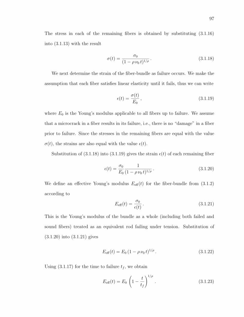
97

The stress in each of the remaining fibers is obtained by substituting (3.1.16)

into (3.1.13) with the result

σ(t) =σ0

(1− ρ ν0 t)1/ρ. (3.1.18)

We next determine the strain of the fiber-bundle as failure occurs. We make the

assumption that each fiber satisfies linear elasticity until it fails, thus we can write

ε(t) =σ(t)

E0

, (3.1.19)

where E0 is the Young’s modulus applicable to all fibers up to failure. We assume

that a microcrack in a fiber results in its failure, i.e., there is no “damage” in a fiber

prior to failure. Since the stresses in the remaining fibers are equal with the value

σ(t), the strains are also equal with the value ε(t).

Substitution of (3.1.18) into (3.1.19) gives the strain ε(t) of each remaining fiber

ε(t) =σ0

E0

1

(1− ρ ν0 t)1/ρ. (3.1.20)

We define an effective Young’s modulus Eeff(t) for the fiber-bundle from (3.1.2)

according to

Eeff(t) =σ0

ε(t). (3.1.21)

This is the Young’s modulus of the bundle as a whole (including both failed and

sound fibers) treated as an equivalent rod failing under tension. Substitution of

(3.1.20) into (3.1.21) gives

Eeff(t) = E0 (1− ρ ν0 t)1/ρ . (3.1.22)

Using (3.1.17) for the time to failure tf , we obtain

Eeff(t) = E0

(1− t

tf

)1/ρ

. (3.1.23)

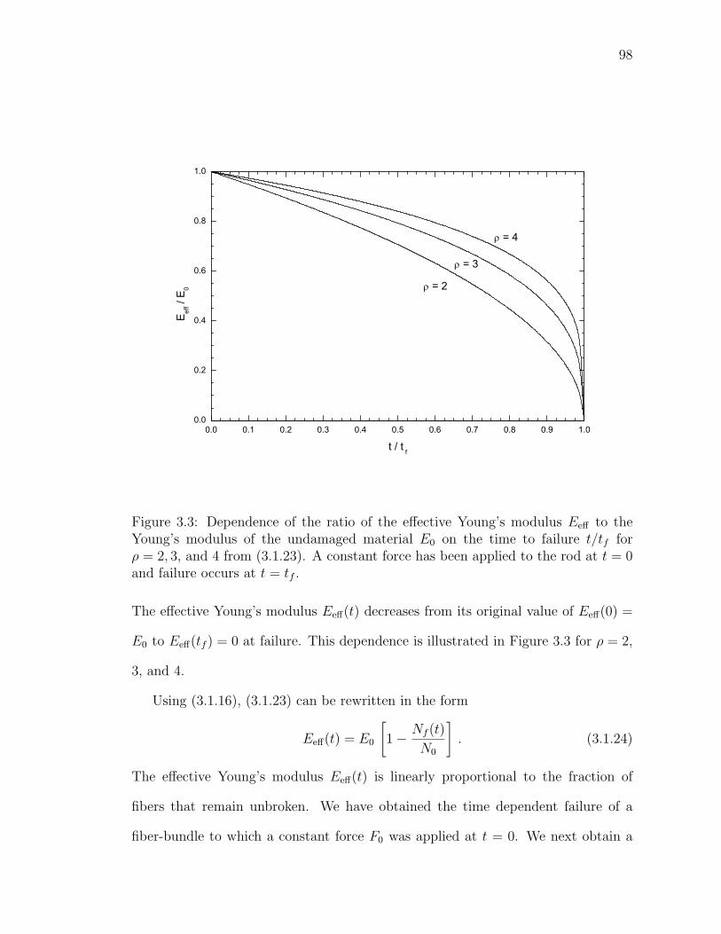
98

0.0 0.1 0.2 0.3 0.4 0.5 0.6 0.7 0.8 0.9 1.00.0

0.2

0.4

0.6

0.8

1.0

ρ = 3

ρ = 4

ρ = 2

E eff /

E0

t / t f

Figure 3.3: Dependence of the ratio of the effective Young’s modulus Eeff to theYoung’s modulus of the undamaged material E0 on the time to failure t/tf forρ = 2, 3, and 4 from (3.1.23). A constant force has been applied to the rod at t = 0and failure occurs at t = tf .

The effective Young’s modulus Eeff(t) decreases from its original value of Eeff(0) =

E0 to Eeff(tf ) = 0 at failure. This dependence is illustrated in Figure 3.3 for ρ = 2,

3, and 4.

Using (3.1.16), (3.1.23) can be rewritten in the form

Eeff(t) = E0

[1− Nf (t)

N0

]. (3.1.24)

The effective Young’s modulus Eeff(t) is linearly proportional to the fraction of

fibers that remain unbroken. We have obtained the time dependent failure of a

fiber-bundle to which a constant force F0 was applied at t = 0. We next obtain a

99

solution to the same problem using the damage model.

3.1.3 Damage model

We have obtained a solution for the strain and effective Young’s modulus during

the failure of a fiber-bundle under a constant applied load. This was basically

a microscopic model in a mean field. We now obtain a solution to the problem

utilizing the macroscopic damage model. We again consider the failure of a rod

under tension. A constant tensional force F0 is applied to the rod at time t = 0.

The damage variable α has been defined in (3.1.3). Equating (3.1.3) and (3.1.24)

we obtain

α(t) =Nf (t)

N0

. (3.1.25)

This definition of damage has been used previously (Krajcinovic, 1996). In our

analogy with the fiber-bundle model, we can interpret the macroscopic damage

variable α(t) to be the fraction of fibers that have failed. We now determine the

time history of strain in a rod using the damage model. We assume that σ0 is

the constant stress applied to the rod at t = 0. For the undamaged material α =

0 and Eeff = E0, failure occurs when α(tf ) = 1 and Eeff(tf ) = 0. Based upon

thermodynamic considerations (Lyakhovsky et al., 1997), the time evolution of the

damage variable can be related to the strain ε(t) by

dα(t)

dt= Aε2(t) (3.1.26)

with A a constant for a constant applied stress. This expression can be regarded

as the lowest order term to emerge from a series in ε; for large strains, higher order

terms may become important. The rate of damage generation is proportional to the

square of the strain in the material.

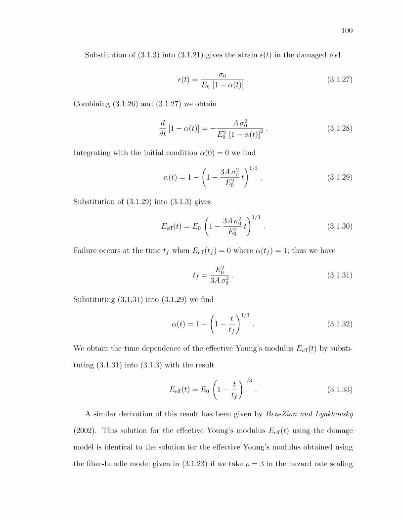
100

Substitution of (3.1.3) into (3.1.21) gives the strain ε(t) in the damaged rod

ε(t) =σ0

E0 [1− α(t)]. (3.1.27)

Combining (3.1.26) and (3.1.27) we obtain

d

dt[1− α(t)] = − Aσ2

0

E20 [1− α(t)]2

. (3.1.28)

Integrating with the initial condition α(0) = 0 we find

α(t) = 1−(

1− 3Aσ20

E20

t

)1/3

. (3.1.29)

Substitution of (3.1.29) into (3.1.3) gives

Eeff(t) = E0

(1− 3Aσ2

0

E20

t

)1/3

. (3.1.30)

Failure occurs at the time tf when Eeff(tf ) = 0 where α(tf ) = 1; thus we have

tf =E2

0

3Aσ20

. (3.1.31)

Substituting (3.1.31) into (3.1.29) we find

α(t) = 1−(

1− t

tf

)1/3

. (3.1.32)

We obtain the time dependence of the effective Young’s modulus Eeff(t) by substi-

tuting (3.1.31) into (3.1.3) with the result

Eeff(t) = E0

(1− t

tf

)1/3

. (3.1.33)

A similar derivation of this result has been given by Ben-Zion and Lyakhovsky

(2002). This solution for the effective Young’s modulus Eeff(t) using the damage

model is identical to the solution for the effective Young’s modulus obtained using

the fiber-bundle model given in (3.1.23) if we take ρ = 3 in the hazard rate scaling

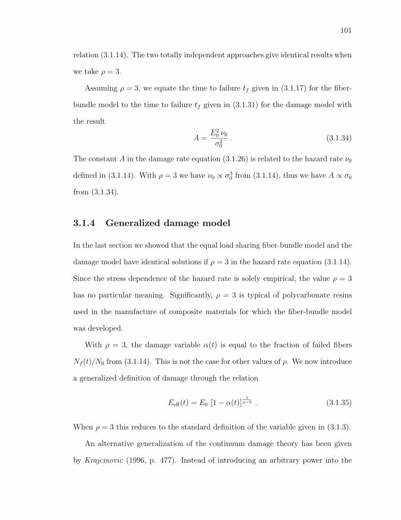
101

relation (3.1.14). The two totally independent approaches give identical results when

we take ρ = 3.

Assuming ρ = 3, we equate the time to failure tf given in (3.1.17) for the fiber-

bundle model to the time to failure tf given in (3.1.31) for the damage model with

the result

A =E2

0 ν0

σ20

. (3.1.34)

The constant A in the damage rate equation (3.1.26) is related to the hazard rate ν0

defined in (3.1.14). With ρ = 3 we have ν0 ∝ σ30 from (3.1.14), thus we have A ∝ σ0

from (3.1.34).

3.1.4 Generalized damage model

In the last section we showed that the equal load sharing fiber-bundle model and the

damage model have identical solutions if ρ = 3 in the hazard rate equation (3.1.14).

Since the stress dependence of the hazard rate is solely empirical, the value ρ = 3

has no particular meaning. Significantly, ρ = 3 is typical of polycarbonate resins

used in the manufacture of composite materials for which the fiber-bundle model

was developed.

With ρ = 3, the damage variable α(t) is equal to the fraction of failed fibers

Nf (t)/N0 from (3.1.14). This is not the case for other values of ρ. We now introduce

a generalized definition of damage through the relation

Eeff(t) = E0 [1− α(t)]1

ρ−2 . (3.1.35)

When ρ = 3 this reduces to the standard definition of the variable given in (3.1.3).

An alternative generalization of the continuum damage theory has been given

by Krajcinovic (1996, p. 477). Instead of introducing an arbitrary power into the

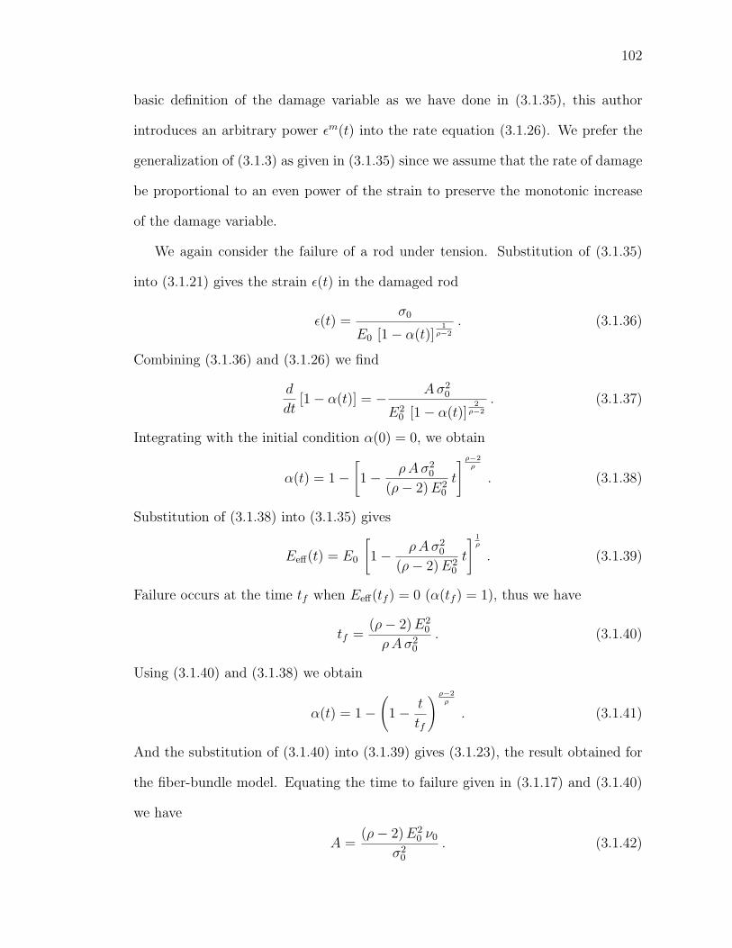
102

basic definition of the damage variable as we have done in (3.1.35), this author

introduces an arbitrary power εm(t) into the rate equation (3.1.26). We prefer the

generalization of (3.1.3) as given in (3.1.35) since we assume that the rate of damage

be proportional to an even power of the strain to preserve the monotonic increase

of the damage variable.

We again consider the failure of a rod under tension. Substitution of (3.1.35)

into (3.1.21) gives the strain ε(t) in the damaged rod

ε(t) =σ0

E0 [1− α(t)]1

ρ−2

. (3.1.36)

Combining (3.1.36) and (3.1.26) we find

d

dt[1− α(t)] = − Aσ2

0

E20 [1− α(t)]

2ρ−2

. (3.1.37)

Integrating with the initial condition α(0) = 0, we obtain

α(t) = 1−[1− ρAσ2

0

(ρ− 2)E20

t

] ρ−2ρ

. (3.1.38)

Substitution of (3.1.38) into (3.1.35) gives

Eeff(t) = E0

[1− ρAσ2

0

(ρ− 2)E20

t

] 1ρ

. (3.1.39)

Failure occurs at the time tf when Eeff(tf ) = 0 (α(tf ) = 1), thus we have

tf =(ρ− 2)E2

0

ρAσ20

. (3.1.40)

Using (3.1.40) and (3.1.38) we obtain

α(t) = 1−(

1− t

tf

) ρ−2ρ

. (3.1.41)

And the substitution of (3.1.40) into (3.1.39) gives (3.1.23), the result obtained for

the fiber-bundle model. Equating the time to failure given in (3.1.17) and (3.1.40)

we have

A =(ρ− 2)E2

0 ν0

σ20

. (3.1.42)

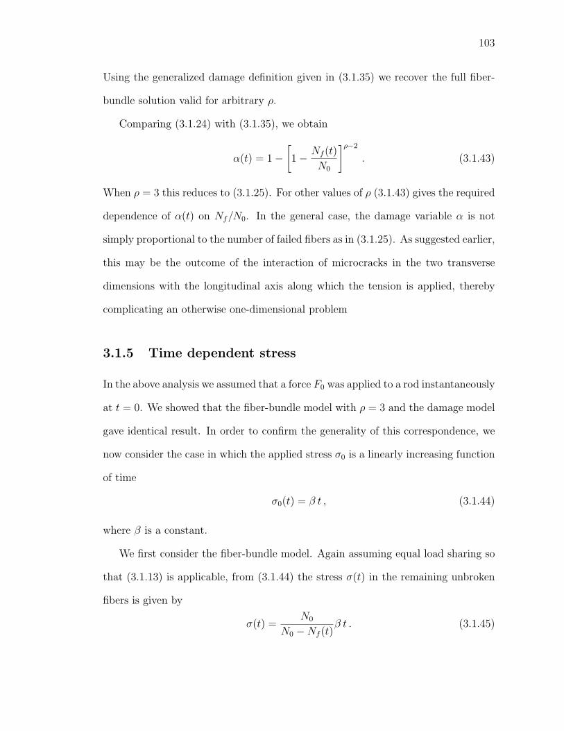
103

Using the generalized damage definition given in (3.1.35) we recover the full fiber-

bundle solution valid for arbitrary ρ.

Comparing (3.1.24) with (3.1.35), we obtain

α(t) = 1−[1− Nf (t)

N0

]ρ−2

. (3.1.43)

When ρ = 3 this reduces to (3.1.25). For other values of ρ (3.1.43) gives the required

dependence of α(t) on Nf/N0. In the general case, the damage variable α is not

simply proportional to the number of failed fibers as in (3.1.25). As suggested earlier,

this may be the outcome of the interaction of microcracks in the two transverse

dimensions with the longitudinal axis along which the tension is applied, thereby

complicating an otherwise one-dimensional problem

3.1.5 Time dependent stress

In the above analysis we assumed that a force F0 was applied to a rod instantaneously

at t = 0. We showed that the fiber-bundle model with ρ = 3 and the damage model

gave identical result. In order to confirm the generality of this correspondence, we

now consider the case in which the applied stress σ0 is a linearly increasing function

of time

σ0(t) = β t , (3.1.44)

where β is a constant.

We first consider the fiber-bundle model. Again assuming equal load sharing so

that (3.1.13) is applicable, from (3.1.44) the stress σ(t) in the remaining unbroken

fibers is given by

σ(t) =N0

N0 −Nf (t)β t . (3.1.45)

104

We again assume that the hazard rate is given by

ν(t) = νf

[σ(t)

σ0(tf )

]ρ

, (3.1.46)

where νf is the hazard rate at the failure stress σ0(tf ) which is given, from (3.1.44),

by

σ0(tf ) = β tf , (3.1.47)

where tf is again the failure time. Substitution of (3.1.47) into (3.1.46) gives

ν(t) = νf

[σ(t)

β tf

]ρ

. (3.1.48)

Combining (3.1.7), (3.1.45), and (3.1.48) we have

d

dt[N0 −Nf (t)] = −νf

(t

tf

)ρNρ

0

[N0 −Nf (t)]ρ−1 . (3.1.49)

Integrating with the initial condition Nf (0) = 0, we find

Nf (t) = N0

[1−

(1− ρ νf

ρ+ 1

tρ+1

tρf

)] 1ρ

(3.1.50)

Failure of the fiber-bundle occurs when Nf (tf ) = N0, the time to failure is given by

tf =ρ+ 1

ρ νf

. (3.1.51)

Comparison of (3.1.51) with (3.1.17) shows that the time to failure for a linearly

increasing stress is ρ+1 times the time to failure for a constant stress. The hazards

rates ν0 in (3.1.17) and νf in (3.1.51) are equivalent since both apply at the time of

failure.

Substitution of (3.1.51) into (3.1.50) gives

Nf (t) = N0

1−

1− ( t

tf

)ρ+1

1ρ

. (3.1.52)

105

Combining (3.1.45), (3.1.47) and (3.1.52) we obtain

σ(t) = σ0(tf )

ttf[

1−(ttf

)ρ+1] 1

ρ

. (3.1.53)

Substitution of (3.1.53) into (3.1.19) gives the strain ε(t) of each remaining fiber

ε(t) = σ0(tf )

ttf

E0

[1−

(ttf

)ρ+1]1/ρ

. (3.1.54)

And the effective Young’s modulus for the fiber-bundle is obtained by substitut-

ing (3.1.54) into (3.1.21)

Eeff(t) = E0

1− ( t

tf

)ρ+11/ρ

. (3.1.55)

Substitution of (3.1.52) into (3.1.55) again gives (3.1.24). As in (3.1.23), the effective

Young’s modulus Eeff(t) decreases from its original value of Eeff(0) = E0 to Eeff(0) =

0 at failure. This dependence is illustrated in Figure 3.4 for ρ = 2, 3, and 4. A

comparison with Figure 3.3 shows that damage develops much later when σ increases

linearly in time than when it is instantaneously applied.

We now consider the damage model with an applied stress that increases linearly

in time. From (3.1.44) and (3.1.47) we have for t ≤ tf

σ0(t) = σ0(tf )t

tf. (3.1.56)

For a constant applied stress σ0 the damage parameter A defined in (3.1.26) is a

constant. The dependence of A on hazard rate ν0 and σ0 has been given in (3.1.34).

For an applied stress that increases linearly with time we replace σ0 in (3.1.34) with

σ0(t) as given by (3.1.56). Further, we replace ν0 in (3.1.34) with ν0(t) which we

obtain from (3.1.46) taking ρ = 3 and assuming ν0(t) is the damage rate at stress

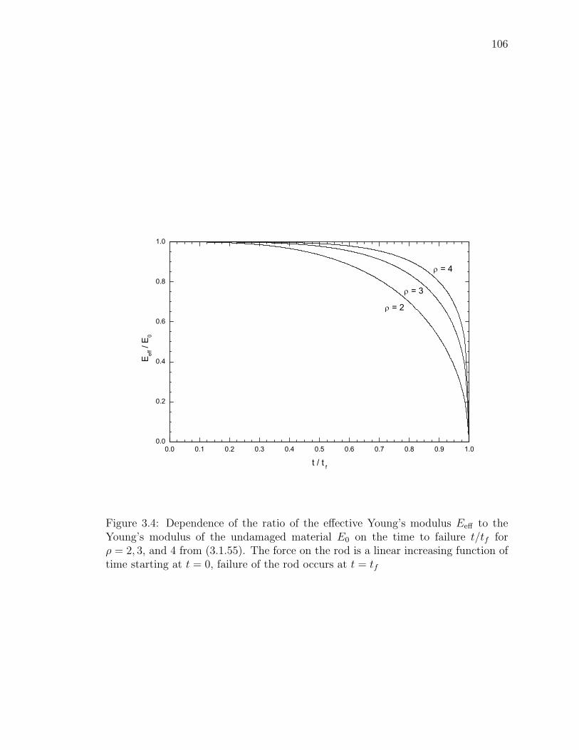
106

0.0 0.1 0.2 0.3 0.4 0.5 0.6 0.7 0.8 0.9 1.00.0

0.2

0.4

0.6

0.8

1.0

ρ = 3

ρ = 4

ρ = 2

E eff /

E0

t / t f

Figure 3.4: Dependence of the ratio of the effective Young’s modulus Eeff to theYoung’s modulus of the undamaged material E0 on the time to failure t/tf forρ = 2, 3, and 4 from (3.1.55). The force on the rod is a linear increasing function oftime starting at t = 0, failure of the rod occurs at t = tf

107

σ0(t). With these substitutions (3.1.34) becomes

A(t) =E2

0 ν0(t)

σ20(t)

=E2

0 νf

σ20(t)

[σ0(t)

σ0(tf )

]3

=E2

0 νf

σ20(tf )

t

tf. (3.1.57)

Substitution of (3.1.57) into (3.1.26) gives

dα(t)

dt=

νf E20

σ20(tf )

t

tfε2(t) . (3.1.58)

And the substitution of (3.1.56) into (3.1.27) gives

ε(t) =σ0(tf ) t

tf E0 [1− α(t)]. (3.1.59)

Using (3.1.59), we are able to rewrite (3.1.58) as follows

dα(t)

dt=

νf

[1− α(t)]2

(t

tf

)3

. (3.1.60)

Integrating with the initial condition α(0) = 0 we obtain

α(t) = 1−(

1− 3νf t4

4t3f

)1/3

. (3.1.61)

Failure occurs when α(tf ) = 1 so that

tf =4

3νf

. (3.1.62)

Combining (3.1.3), (3.1.61), and (3.1.62) we get

Eeff(t) = E0

1− ( t

tf

)41/3

(3.1.63)

If we take ρ = 3 we find (3.1.62) is identical to (3.1.51) and that (3.1.63) is identical

to (3.1.33). Once again, we find that the fiber-bundle model and the damage model

give identical results if ρ = 3. Thus, we see that the time-dependent stress model is

a rescaled version of the constant stress model.

108

3.1.6 Acoustic emission events

A characteristic of materials experiencing “damage” are acoustic emission events.

For a solid material stressed beyond its elastic limit the acoustic emission events are

associated with microcracks. For a fibrous material the acoustic emission events are

associated with the failure of one or more fibers.

We now obtain an expression for the energy flux associated with the acoustic

emission events from a fiber-bundle as fibers break using the model considered above.

In our fiber-bundle model we assume that individual fibers satisfy linear elasticity

until failure. Thus the stored elastic energy in a single fiber ef (t) at the time of

failure is given by

ef (t) =1

2Vf E0 ε

2(t) , (3.1.64)

where Vf is the volume of the fiber, E0 is the Young’s modulus of the fiber, and ε is

the strain in the fiber given by (3.1.20). We assume that when a fiber fails, a fraction

ηa of the stored elastic energy given by (3.1.64) is the energy in the acoustic emission

event. The efficiency ηa is analogous to the seismic efficiency ηs, the fraction of the

stored elastic energy lost during an earthquake that is radiated in the seismic waves

generated by earthquake. In both earthquakes and in acoustic emission events from

damaged materials, energy is also used to rupture material and in some cases is

dissipated in frictional heating. We assume that the acoustic emission efficiency ηa

is a constant.

The rate at which energy is lost by acoustic emission events is given by

defa(t)

dt= ηa ef (t)

dNf (t)

dt, (3.1.65)

where efa(t) is the energy associated with the acoustic emission event and ef (t) is

109

the stored elastic energy in a fiber. Substituting (3.1.64) into (3.1.65) we obtain

defa(t)

dt=

1

2ηa Vf E0 ε

2(t)dNf (t)

dt. (3.1.66)

Since the total volume of fibers is N0Vf , the rate of energy loss in acoustic emission

events per unit volume of material ea(t) is given by

dea(t)

dt=

1

2ηaE0 ε

2(t)

N0

dNf (t)

dt. (3.1.67)

From (3.1.15), the rate at which fibers fail can be written

dNf (t)

dt=

ν0Nρ0

[N0 −Nf (t)]ρ−1(3.1.68)

and, from (3.1.16) and (3.1.20), we have the fiber strain at its time of failure t

ε(t) =σ0

E0

[N0

N0 −Nf (t)

]. (3.1.69)

Using (3.1.68) and (3.1.69), we can rewrite (3.1.67) in the form

dea(t)

dt=

1

2ηaν0 σ

20

E0

[N0

N0 −Nf (t)

]ρ+1

. (3.1.70)

Combining (3.1.16), (3.1.17), and (3.1.70) we obtain

dea(t)

dt=ηa ν0 σ

20

2E0

1(1− t

tf

) ρ+1ρ

. (3.1.71)

This is the rate at which energy is radiated in acoustic emission events during the

failure of a fiber-bundle.

While the rate at which energy is lost in acoustic emission events can be deter-

mined from the microscopic fiber-bundle model, this is not the case for the macro-

scopic damage model. We now use our analogy between the two models to determine

a relationship between the energy addition associated with damage and the loss due

to acoustic emission events.

110

We use the damage model to determine the rate at which work is being done on

a rod. Since the stress on the rod σ0 is constant we have

dw(t)

dt= σ0

dε(t)

dt, (3.1.72)

where w(t) is the work per unit volume done on the rod. Taking the derivative

of (3.1.27) we obtain

dε(t)

dt=

σ0

E0 [1− α(t)]2dα(t)

dt. (3.1.73)

Substitution of (3.1.26), (3.1.27) and (3.1.73) into (3.1.72) gives

dw(t)

dt=

Aσ40

E30 [1− α(t)]4

. (3.1.74)

Upon substitution of (3.1.32) and (3.1.34) into (3.1.74) we have

dw(t)

dt=ν0 σ

20

E0

1(1− t

tf

)4/3. (3.1.75)

This result was previously obtained by Ben-Zion and Lyakhovsky (2002). Compar-

ing (3.1.75) with (3.1.71), noting that ρ = 3 in our analogy, we find that

dea(t)

dt=ηa

2

dw(t)

dt. (3.1.76)

If the acoustic efficiency is ηa = 1, we find that one-half of the energy that is added

to the damaged medium is lost in acoustic emission events.

We next determine the energy in acoustic emission when the applied stress

is increasing linearly in time as given by (3.1.44). Combining (3.1.49), (3.1.67),

and (3.1.69), we obtain

dea(t)

dt=ηa νf σ

20

2E0

(t

tf

)ρ [N0

N0 −Nf (t)

]ρ+1

. (3.1.77)

Using (3.1.52) one obtains

dea(t)

dt=ηa νf σ

20

2E0

(t

tf

)ρ1[

1−(

ttf

)ρ+1] ρ+1

ρ

. (3.1.78)

111

In the vicinity of rupture, we have (1− t/tf ) 1. In this limit, we obtain from

(3.1.78) that

dea(t)

dt∝ 1(

1− ttf

) ρ+1ρ

. (3.1.79)

Thus, the scaling in the vicinity of rupture is the same as that obtained for the

constant pressure result given in (3.1.71).

We now compare the predicted acoustic emission associated with material failure

with experiments. Guarino et al. (1998, 1999) studied the failure of circular panels

(220 mm diameter, 3-5 mm thickness) of chipboard and fiberglass. A differential

pressure was applied across the panels until they failed. Acoustic emission events

were carefully monitored. For these relatively thin panels, bending stresses were

negligible and the panels failed under tension (a mode I fracture). The acoustic

emission events were used to locate the associated microcracks. Initially, the mi-

crocracks appeared to be randomly distributed across the panel. As the pressure

difference was increased, the microcracks localized in the region where the final rup-

ture occurred. In the first series of experiments given by Guarino et al. (1998) the

applied pressure difference (differential stress) was increased linearly with time in

accordance with (3.1.54).

These authors determined the cumulative energy associated with acoustic emis-

sion events prior to rupture. The observed dependence of ea/etot on (1 − P/Pf ) is

given in Figure 3.5a where ea is the cumulative acoustic energy at time t and etot is

the total acoustic energy at rupture (t = tf ). Clear power-law behavior is observed

for (1 − P/Pf ) less than about 0.1. The slope is ea ∝ (1 − P/Pf )−0.27±0.05. This

is equivalent to having dea/dt ∝ (1 − P/Pf )−1.27±0.05. This result is in agreement

with the predicted dependence given in (3.1.79) if we take ρ = 3.7. Similar results

were obtained by Johansen and Sornette (2000) who studied the failure of spherical

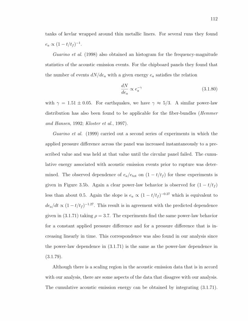
112

tanks of kevlar wrapped around thin metallic liners. For several runs they found

ea ∝ (1− t/tf )−1.

Guarino et al. (1998) also obtained an histogram for the frequency-magnitude

statistics of the acoustic emission events. For the chipboard panels they found that

the number of events dN/dea with a given energy ea satisfies the relation

dN

dea

∝ e−γa (3.1.80)

with γ = 1.51 ± 0.05. For earthquakes, we have γ ≈ 5/3. A similar power-law

distribution has also been found to be applicable for the fiber-bundles (Hemmer

and Hansen, 1992; Kloster et al., 1997).

Guarino et al. (1999) carried out a second series of experiments in which the

applied pressure difference across the panel was increased instantaneously to a pre-

scribed value and was held at that value until the circular panel failed. The cumu-

lative energy associated with acoustic emission events prior to rupture was deter-

mined. The observed dependence of ea/etot on (1 − t/tf ) for these experiments is

given in Figure 3.5b. Again a clear power-law behavior is observed for (1 − t/tf )

less than about 0.5. Again the slope is ea ∝ (1 − t/tf )−0.27 which is equivalent to

dea/dt ∝ (1− t/tf )−1.27. This result is in agreement with the predicted dependence

given in (3.1.71) taking ρ = 3.7. The experiments find the same power-law behavior

for a constant applied pressure difference and for a pressure difference that is in-

creasing linearly in time. This correspondence was also found in our analysis since

the power-law dependence in (3.1.71) is the same as the power-law dependence in

(3.1.79).

Although there is a scaling region in the acoustic emission data that is in accord

with our analysis, there are some aspects of the data that disagree with our analysis.

The cumulative acoustic emission energy can be obtained by integrating (3.1.71).

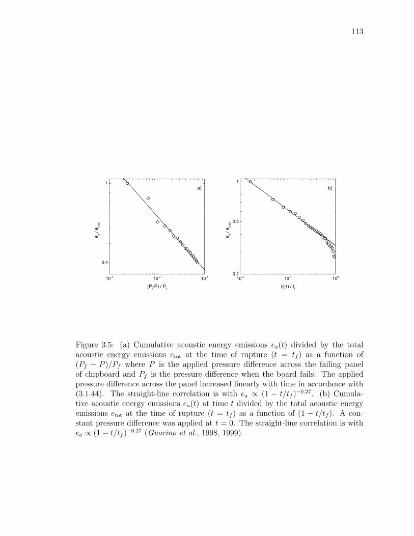
113

10-3 10-2 10-1

0.4

1a)

e a / e

tota

l

(Pf-P) / Pf

10-2 10-1 1000.2

0.5

1b)

e a / e

tota

l

(tf-t) / tf

Figure 3.5: (a) Cumulative acoustic energy emissions ea(t) divided by the totalacoustic energy emissions etot at the time of rupture (t = tf ) as a function of(Pf − P )/Pf where P is the applied pressure difference across the failing panelof chipboard and Pf is the pressure difference when the board fails. The appliedpressure difference across the panel increased linearly with time in accordance with(3.1.44). The straight-line correlation is with ea ∝ (1 − t/tf )

−0.27. (b) Cumula-tive acoustic energy emissions ea(t) at time t divided by the total acoustic energyemissions etot at the time of rupture (t = tf ) as a function of (1 − t/tf ). A con-stant pressure difference was applied at t = 0. The straight-line correlation is withea ∝ (1− t/tf )

−0.27 (Guarino et al., 1998, 1999).

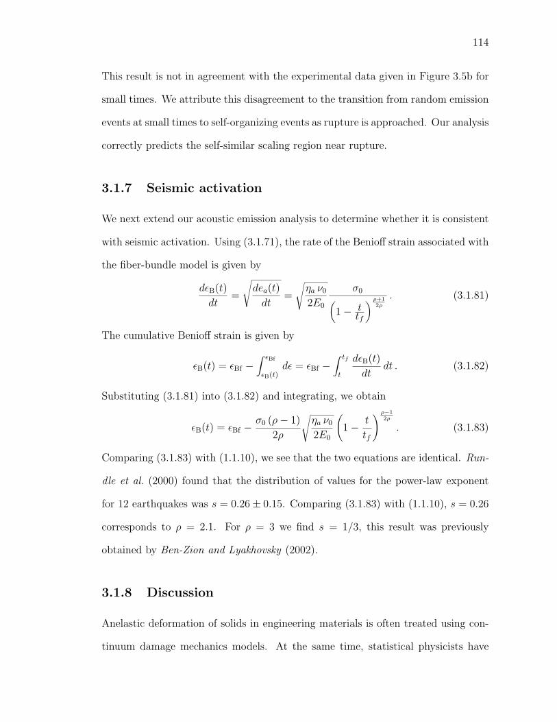
114

This result is not in agreement with the experimental data given in Figure 3.5b for

small times. We attribute this disagreement to the transition from random emission

events at small times to self-organizing events as rupture is approached. Our analysis

correctly predicts the self-similar scaling region near rupture.

3.1.7 Seismic activation

We next extend our acoustic emission analysis to determine whether it is consistent

with seismic activation. Using (3.1.71), the rate of the Benioff strain associated with

the fiber-bundle model is given by

dεB(t)

dt=

√dea(t)

dt=

√ηa ν0

2E0

σ0(1− t

tf

) ρ+12ρ

. (3.1.81)

The cumulative Benioff strain is given by

εB(t) = εBf −∫ εBf

εB(t)dε = εBf −

∫ tf

t

dεB(t)

dtdt . (3.1.82)

Substituting (3.1.81) into (3.1.82) and integrating, we obtain

εB(t) = εBf −σ0 (ρ− 1)

2ρ

√ηa ν0

2E0

(1− t

tf

) ρ−12ρ

. (3.1.83)

Comparing (3.1.83) with (1.1.10), we see that the two equations are identical. Run-

dle et al. (2000) found that the distribution of values for the power-law exponent

for 12 earthquakes was s = 0.26± 0.15. Comparing (3.1.83) with (1.1.10), s = 0.26

corresponds to ρ = 2.1. For ρ = 3 we find s = 1/3, this result was previously

obtained by Ben-Zion and Lyakhovsky (2002).

3.1.8 Discussion

Anelastic deformation of solids in engineering materials is often treated using con-

tinuum damage mechanics models. At the same time, statistical physicists have

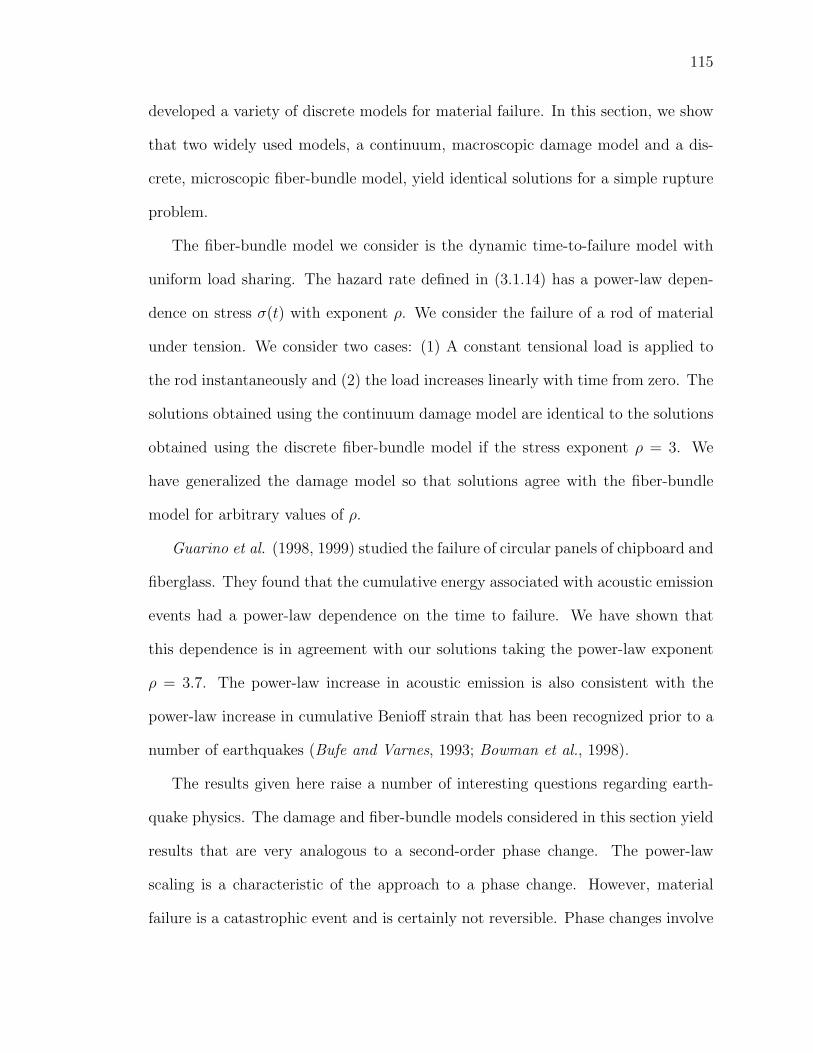
115

developed a variety of discrete models for material failure. In this section, we show

that two widely used models, a continuum, macroscopic damage model and a dis-

crete, microscopic fiber-bundle model, yield identical solutions for a simple rupture

problem.

The fiber-bundle model we consider is the dynamic time-to-failure model with

uniform load sharing. The hazard rate defined in (3.1.14) has a power-law depen-

dence on stress σ(t) with exponent ρ. We consider the failure of a rod of material

under tension. We consider two cases: (1) A constant tensional load is applied to

the rod instantaneously and (2) the load increases linearly with time from zero. The

solutions obtained using the continuum damage model are identical to the solutions

obtained using the discrete fiber-bundle model if the stress exponent ρ = 3. We

have generalized the damage model so that solutions agree with the fiber-bundle

model for arbitrary values of ρ.

Guarino et al. (1998, 1999) studied the failure of circular panels of chipboard and

fiberglass. They found that the cumulative energy associated with acoustic emission

events had a power-law dependence on the time to failure. We have shown that

this dependence is in agreement with our solutions taking the power-law exponent

ρ = 3.7. The power-law increase in acoustic emission is also consistent with the

power-law increase in cumulative Benioff strain that has been recognized prior to a

number of earthquakes (Bufe and Varnes, 1993; Bowman et al., 1998).

The results given here raise a number of interesting questions regarding earth-

quake physics. The damage and fiber-bundle models considered in this section yield

results that are very analogous to a second-order phase change. The power-law

scaling is a characteristic of the approach to a phase change. However, material

failure is a catastrophic event and is certainly not reversible. Phase changes involve

116

a tuning parameter such as temperature or magnetic field.

Rundle et al. (2000) previously considered precursory seismic activation in terms

of a self-organizing spinodal behavior. A typical first-order phase change is the

boiling of water. Ordinarily water at a specified temperature is heated at the boiling

temperature and water is transformed to steam at this temperature as heat is added.

This is an equilibrium process. However, it is possible to superheat water into the

spinodal region of the phase plane. This superheated water is metastable and time

dependent boiling will occur. We suggest that the nonequilibrium irreversible boiling

of water is analogous to the time dependent failure considered in this paper. Rundle

et al. (2000) obtained a power-law scaling of seismic activation using spinodal theory

very similar to the scaling given above.

3.2 Aftershocks and stress relaxation

Solutions to one-dimensional damage problems require the simultaneous solution of

(3.1.3)–(3.1.6). In general it is required that either the stress or the strain on the

sample be specified. We will consider three examples:

1) We assume that a constant strain ε0 is applied instantaneously at t = 0. If

ε0 ≤ εy no damage occurs and the stress is given by (3.1.1). If ε0 > εy the

material is strained elastically into the metastable region along the path ABD

in Figure 1.6. The strain is maintained at ε0 as damage occurs. Because of

the damage the stress on the sample relaxes from the initial value σ0 to the

yield stress σy. This stress relaxation takes place along path DH illustrated in

Figure 1.6. Our solution will give the time dependence of the damage variable

α(t) and stress σ(t) during the relaxation. We discuss the application of this

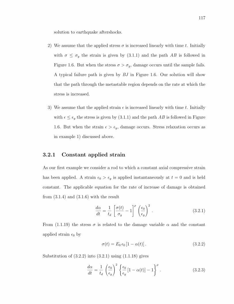
117

solution to earthquake aftershocks.

2) We assume that the applied stress σ is increased linearly with time t. Initially

with σ ≤ σy the strain is given by (3.1.1) and the path AB is followed in

Figure 1.6. But when the stress σ > σy, damage occurs until the sample fails.

A typical failure path is given by BJ in Figure 1.6. Our solution will show

that the path through the metastable region depends on the rate at which the

stress is increased.

3) We assume that the applied strain ε is increased linearly with time t. Initially

with ε ≤ εy the stress is given by (3.1.1) and the path AB is followed in Figure

1.6. But when the strain ε > εy, damage occurs. Stress relaxation occurs as

in example 1) discussed above.

3.2.1 Constant applied strain

As our first example we consider a rod to which a constant axial compressive strain

has been applied. A strain ε0 > εy is applied instantaneously at t = 0 and is held

constant. The applicable equation for the rate of increase of damage is obtained

from (3.1.4) and (3.1.6) with the result

dα

dt=

1

td

[σ(t)

σy

− 1

]ρ (ε0εy

)2

. (3.2.1)

From (1.1.19) the stress σ is related to the damage variable α and the constant

applied strain ε0 by

σ(t) = E0 ε0 [1− α(t)] . (3.2.2)

Substitution of (3.2.2) into (3.2.1) using (1.1.18) gives

dα

dt=

1

td

(ε0εy

)2 ε0εy

[1− α(t)]− 1

ρ

. (3.2.3)

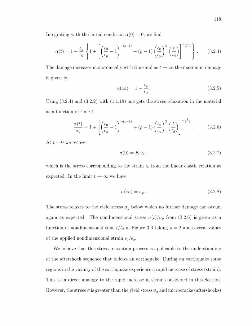
118

Integrating with the initial condition α(0) = 0, we find

α(t) = 1− εyε0

1 +

(ε0εy− 1

)−(ρ−1)

+ (ρ− 1)

(ε0εy

)3 (t

td

)− 1ρ−1

. (3.2.4)

The damage increases monotonically with time and as t→∞ the maximum damage

is given by

α(∞) = 1− εyε0. (3.2.5)

Using (3.2.4) and (3.2.2) with (1.1.18) one gets the stress relaxation in the material

as a function of time t

σ(t)

σy

= 1 +

(ε0εy− 1

)−(ρ−1)

+ (ρ− 1)

(ε0εy

)3 (t

td

)− 1ρ−1

. (3.2.6)

At t = 0 we recover

σ(0) = E0 ε0 , (3.2.7)

which is the stress corresponding to the strain ε0 from the linear elastic relation as

expected. In the limit t→∞ we have

σ(∞) = σy . (3.2.8)

The stress relaxes to the yield stress σy below which no further damage can occur,

again as expected. The nondimensional stress σ(t)/σy from (3.2.6) is given as a

function of nondimensional time t/td in Figure 3.6 taking ρ = 2 and several values

of the applied nondimensional strain ε0/εy.

We believe that this stress relaxation process is applicable to the understanding

of the aftershock sequence that follows an earthquake. During an earthquake some

regions in the vicinity of the earthquake experience a rapid increase of stress (strain).

This is in direct analogy to the rapid increase in strain considered in this Section.

However, the stress σ is greater than the yield stress σy and microcracks (aftershocks)

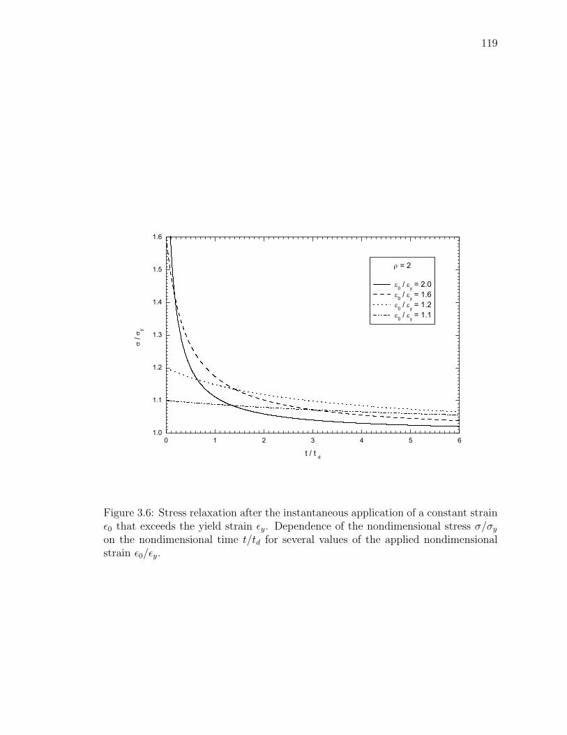
119

0 1 2 3 4 5 61.0

1.1

1.2

1.3

1.4

1.5

1.6

σ / σ

y

t / t d

ρ = 2

ε0 / εy = 2.0 ε0 / εy = 1.6 ε0 / εy = 1.2 ε0 / εy = 1.1

Figure 3.6: Stress relaxation after the instantaneous application of a constant strainε0 that exceeds the yield strain εy. Dependence of the nondimensional stress σ/σy

on the nondimensional time t/td for several values of the applied nondimensionalstrain ε0/εy.

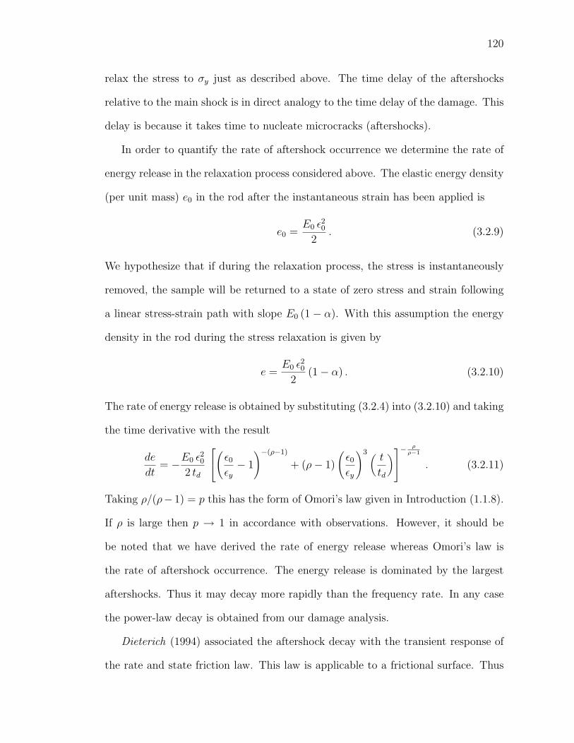
120

relax the stress to σy just as described above. The time delay of the aftershocks

relative to the main shock is in direct analogy to the time delay of the damage. This

delay is because it takes time to nucleate microcracks (aftershocks).

In order to quantify the rate of aftershock occurrence we determine the rate of

energy release in the relaxation process considered above. The elastic energy density

(per unit mass) e0 in the rod after the instantaneous strain has been applied is

e0 =E0 ε

20

2. (3.2.9)

We hypothesize that if during the relaxation process, the stress is instantaneously

removed, the sample will be returned to a state of zero stress and strain following

a linear stress-strain path with slope E0 (1 − α). With this assumption the energy

density in the rod during the stress relaxation is given by

e =E0 ε

20

2(1− α) . (3.2.10)

The rate of energy release is obtained by substituting (3.2.4) into (3.2.10) and taking

the time derivative with the result

de

dt= −E0 ε

20

2 td

(ε0εy− 1

)−(ρ−1)

+ (ρ− 1)

(ε0εy

)3 (t

td

)−ρ

ρ−1

. (3.2.11)

Taking ρ/(ρ− 1) = p this has the form of Omori’s law given in Introduction (1.1.8).

If ρ is large then p → 1 in accordance with observations. However, it should be

be noted that we have derived the rate of energy release whereas Omori’s law is

the rate of aftershock occurrence. The energy release is dominated by the largest

aftershocks. Thus it may decay more rapidly than the frequency rate. In any case

the power-law decay is obtained from our damage analysis.

Dieterich (1994) associated the aftershock decay with the transient response of

the rate and state friction law. This law is applicable to a frictional surface. Thus

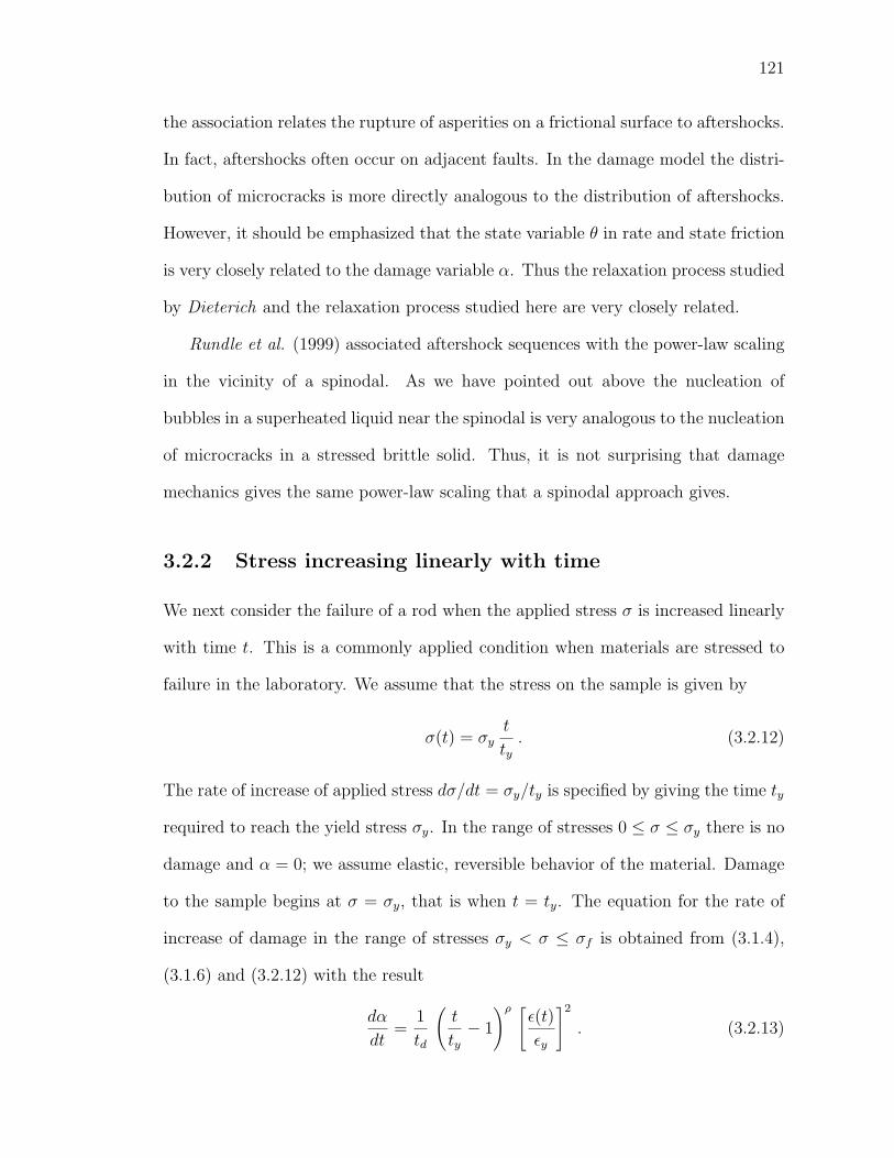
121

the association relates the rupture of asperities on a frictional surface to aftershocks.

In fact, aftershocks often occur on adjacent faults. In the damage model the distri-

bution of microcracks is more directly analogous to the distribution of aftershocks.

However, it should be emphasized that the state variable θ in rate and state friction

is very closely related to the damage variable α. Thus the relaxation process studied

by Dieterich and the relaxation process studied here are very closely related.

Rundle et al. (1999) associated aftershock sequences with the power-law scaling

in the vicinity of a spinodal. As we have pointed out above the nucleation of

bubbles in a superheated liquid near the spinodal is very analogous to the nucleation

of microcracks in a stressed brittle solid. Thus, it is not surprising that damage

mechanics gives the same power-law scaling that a spinodal approach gives.

3.2.2 Stress increasing linearly with time

We next consider the failure of a rod when the applied stress σ is increased linearly

with time t. This is a commonly applied condition when materials are stressed to

failure in the laboratory. We assume that the stress on the sample is given by

σ(t) = σyt

ty. (3.2.12)

The rate of increase of applied stress dσ/dt = σy/ty is specified by giving the time ty

required to reach the yield stress σy. In the range of stresses 0 ≤ σ ≤ σy there is no

damage and α = 0; we assume elastic, reversible behavior of the material. Damage

to the sample begins at σ = σy, that is when t = ty. The equation for the rate of

increase of damage in the range of stresses σy < σ ≤ σf is obtained from (3.1.4),

(3.1.6) and (3.2.12) with the result

dα

dt=

1

td

(t

ty− 1

)ρ [ε(t)

εy

]2

. (3.2.13)

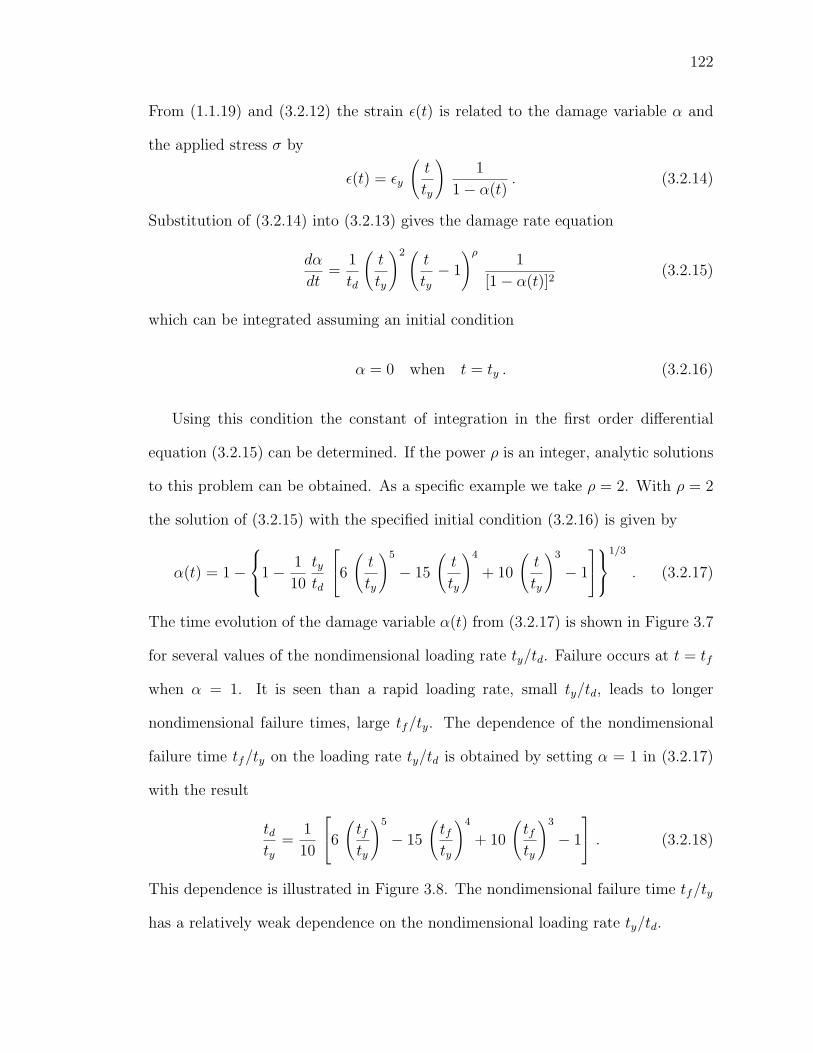
122

From (1.1.19) and (3.2.12) the strain ε(t) is related to the damage variable α and

the applied stress σ by

ε(t) = εy

(t

ty

)1

1− α(t). (3.2.14)

Substitution of (3.2.14) into (3.2.13) gives the damage rate equation

dα

dt=

1

td

(t

ty

)2 (t

ty− 1

)ρ1

[1− α(t)]2(3.2.15)

which can be integrated assuming an initial condition

α = 0 when t = ty . (3.2.16)

Using this condition the constant of integration in the first order differential

equation (3.2.15) can be determined. If the power ρ is an integer, analytic solutions

to this problem can be obtained. As a specific example we take ρ = 2. With ρ = 2

the solution of (3.2.15) with the specified initial condition (3.2.16) is given by

α(t) = 1−

1− 1

10

tytd

6 ( t

ty

)5

− 15

(t

ty

)4

+ 10

(t

ty

)3

− 1

1/3

. (3.2.17)

The time evolution of the damage variable α(t) from (3.2.17) is shown in Figure 3.7

for several values of the nondimensional loading rate ty/td. Failure occurs at t = tf

when α = 1. It is seen than a rapid loading rate, small ty/td, leads to longer

nondimensional failure times, large tf/ty. The dependence of the nondimensional

failure time tf/ty on the loading rate ty/td is obtained by setting α = 1 in (3.2.17)

with the result

tdty

=1

10

6 (tfty

)5

− 15

(tfty

)4

+ 10

(tfty

)3

− 1

. (3.2.18)

This dependence is illustrated in Figure 3.8. The nondimensional failure time tf/ty

has a relatively weak dependence on the nondimensional loading rate ty/td.

123

1.0 1.2 1.4 1.6 1.8 2.0 2.2 2.40.0

0.2

0.4

0.6

0.8

1.0

ty / td = 100.0 ty / td = 10.0 ty / td = 1.0 ty / td = 0.1

α

t / ty

Figure 3.7: Dependence of the damage variable α on the nondimensional time t/tdfor several values of the nondimensional loading rate ty/td. The applied stress isincreased linearly with time. Failure occurs when α = 1.

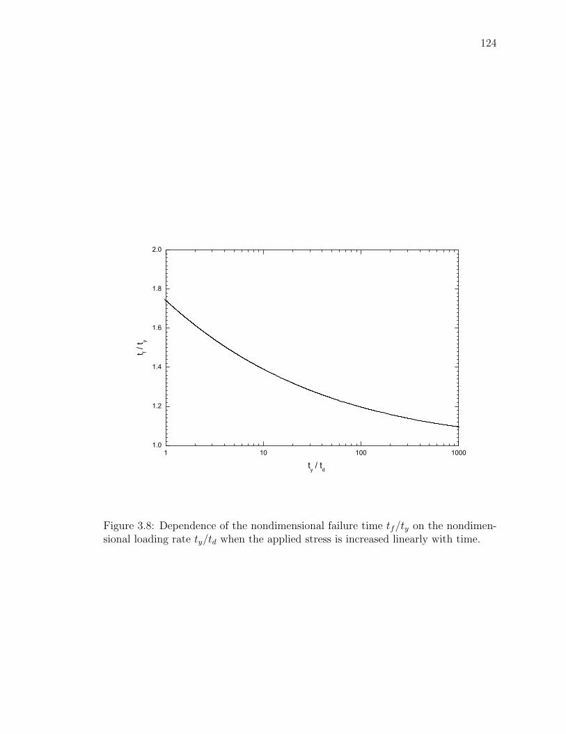
124

1.0

1.2

1.4

1.6

1.8

2.0

1 10 100 1000

ty / td

t f / t y

Figure 3.8: Dependence of the nondimensional failure time tf/ty on the nondimen-sional loading rate ty/td when the applied stress is increased linearly with time.

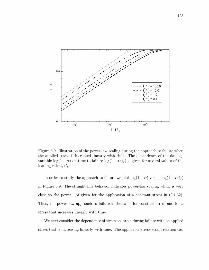
125

10-3 10-2 10-10.1

0.5

1

ty / td = 100.0 ty / td = 10.0 ty / td = 1.0 ty / td = 0.1

1 −

α

1 - t / tf

Figure 3.9: Illustration of the power-law scaling during the approach to failure whenthe applied stress is increased linearly with time. The dependence of the damagevariable log(1− α) on time to failure log(1− t/tf ) is given for several values of theloading rate ty/td.

In order to study the approach to failure we plot log(1− α) versus log(1− t/tf )

in Figure 3.9. The straight line behavior indicates power-law scaling which is very

close to the power 1/3 given for the application of a constant stress in (3.1.32).

Thus, the power-law approach to failure is the same for constant stress and for a

stress that increases linearly with time.

We next consider the dependence of stress on strain during failure with an applied

stress that is increasing linearly with time. The applicable stress-strain relation can

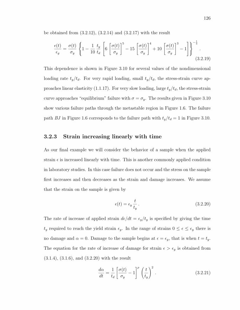
126

be obtained from (3.2.12), (3.2.14) and (3.2.17) with the result

ε(t)

εy=σ(t)

σy

1− 1

10

tytd

6 [σ(t)

σy

]5

− 15

[σ(t)

σy

]4

+ 10

[σ(t)

σy

]3

− 1

− 1

3

.

(3.2.19)

This dependence is shown in Figure 3.10 for several values of the nondimensional

loading rate ty/td. For very rapid loading, small ty/td, the stress-strain curve ap-

proaches linear elasticity (1.1.17). For very slow loading, large ty/td, the stress-strain

curve approaches “equilibrium” failure with σ = σy. The results given in Figure 3.10

show various failure paths through the metastable region in Figure 1.6. The failure

path BJ in Figure 1.6 corresponds to the failure path with ty/td = 1 in Figure 3.10.

3.2.3 Strain increasing linearly with time

As our final example we will consider the behavior of a sample when the applied

strain ε is increased linearly with time. This is another commonly applied condition

in laboratory studies. In this case failure does not occur and the stress on the sample

first increases and then decreases as the strain and damage increases. We assume

that the strain on the sample is given by

ε(t) = εyt

ty. (3.2.20)

The rate of increase of applied strain dε/dt = εy/ty is specified by giving the time

ty required to reach the yield strain εy. In the range of strains 0 ≤ ε ≤ εy there is

no damage and α = 0. Damage to the sample begins at ε = εy, that is when t = ty.

The equation for the rate of increase of damage for strain ε > εy is obtained from

(3.1.4), (3.1.6), and (3.2.20) with the result

dα

dt=

1

td

[σ(t)

σy

− 1

]ρ (t

ty

)2

. (3.2.21)

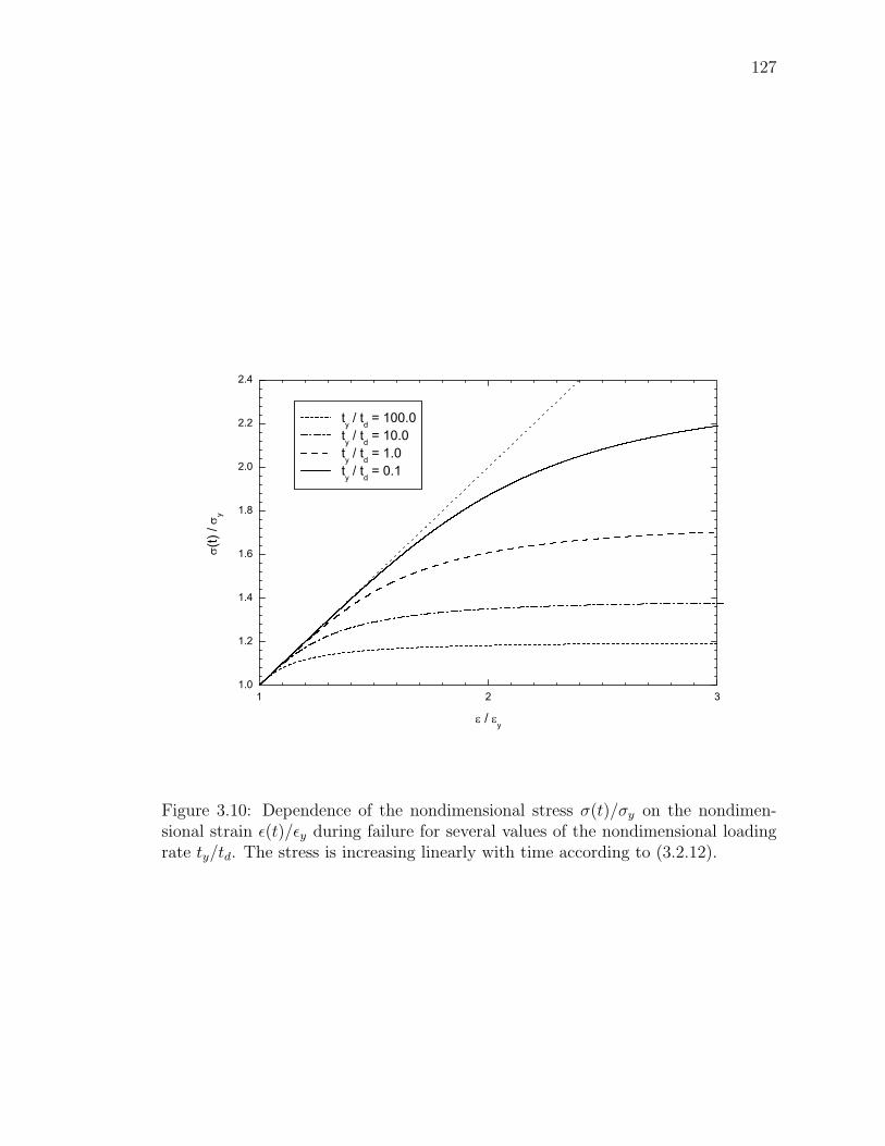
127

1 2 31.0

1.2

1.4

1.6

1.8

2.0

2.2

2.4

ty / td = 100.0 ty / td = 10.0 ty / td = 1.0 ty / td = 0.1

σ(t)

/ σy

ε / εy

Figure 3.10: Dependence of the nondimensional stress σ(t)/σy on the nondimen-sional strain ε(t)/εy during failure for several values of the nondimensional loadingrate ty/td. The stress is increasing linearly with time according to (3.2.12).

128

1 2 3 4 5 60.0

0.2

0.4

0.6

0.8

1.0

ty / td = 100.0 ty / td = 10.0 ty / td = 1.0 ty / td = 0.1

α

t / ty

Figure 3.11: Dependence of the damage variable α on the nondimensional time t/tyfor several values of the nondimensional loading rate ty/td. The applied strain isincreased linearly with time.

From (1.1.19) and (3.2.20) the stress σ(t) is related to the damage variable α(t) and

the applied strain ε(t) by

σ(t) = σy [1− α(t)]ε(t)

εy= σy [1− α(t)]

t

ty, (3.2.22)

Using (3.2.22) we are able to rewrite the damage rate equation (3.2.21) in the fol-

lowing form

dα

dt=

1

td

[1− α(t)]

t

ty− 1

ρ (t

ty

)2

. (3.2.23)

The solution to equation (3.2.23) can be obtained only numerically. The damage

starts to develop at time t = ty when the stress σ equals the yield stress σy. Therefore

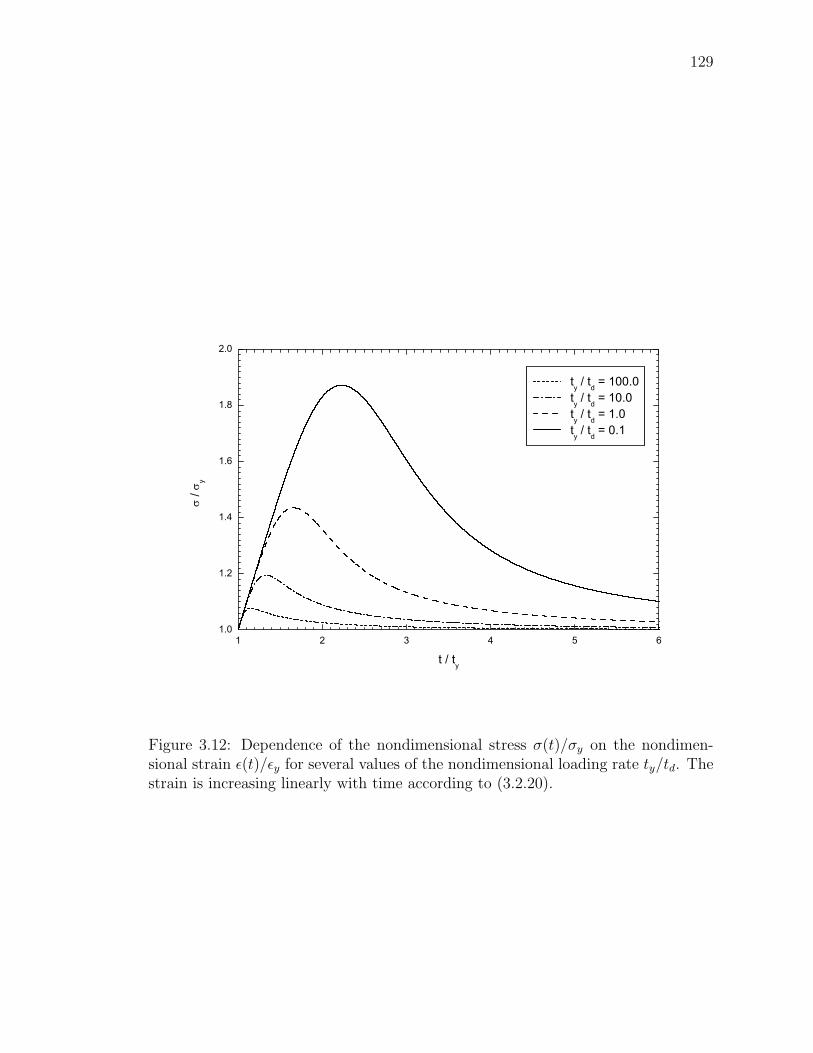
129

1 2 3 4 5 61.0

1.2

1.4

1.6

1.8

2.0

ty / td = 100.0 ty / td = 10.0 ty / td = 1.0 ty / td = 0.1

σ / σ

y

t / ty

Figure 3.12: Dependence of the nondimensional stress σ(t)/σy on the nondimen-sional strain ε(t)/εy for several values of the nondimensional loading rate ty/td. Thestrain is increasing linearly with time according to (3.2.20).

130

we use the initial condition α(ty) = 0. The time evolution of the damage variable

α(t) from the numerical solutions of (3.2.23) is shown in Figure 3.11 for several values

of the nondimensional loading rate ty/td. In the damage model failure does not occur

since α → 1 only as t → ∞. Our numerical solutions also give the dependence

of stress on strain when the applied stress is increasing linearly with time. This

dependence is shown in Figure 3.12 for several values of the nondimensional loading

rate ty/td. It is seen that the stress first increases to a maximum value and then

decreases with increasing strain (time). This stress relaxation is similar to that

obtained in Section 3.2.1 with the instantaneous application of a constant strain.

The maximum stress increases with increasing loading rate, small ty/td.

3.2.4 Discussion

Each type of solid requires its own formulation of constitutive equations which de-

fine the evolution of damage. A relevant measure as to the applicability of damage

mechanics would be the amount of “disorder” in the solid. A pure crystalline ma-

terial would have minimum disorder. Dislocations and microcracks would increase

the disorder. Brittle composite materials have considerable built in disorder. It has

been shown (Krajcinovic, 1996; Turcotte et al., 2002) that there is a close associa-

tion between damage mechanics and the failure of fiber-bundles. Fiber-bundles are

an accepted model for the failure of composite materials. It is clear that the upper

continental crust has a high degree of disorder in terms of preexisting faults and

joints. Thus, it is reasonable to hypothesize that damage mechanics is applicable to

the continental crust.

Damage mechanics is a quasi-empirical approach to the deformation of a brittle

solid. However, the dependence of rate of damage generation on strain and stress

131

(3.1.4) has a thermodynamic basis (Kachanov, 1986; Krajcinovic, 1996; Lyakhovsky

et al., 1997). The analogy we have made between phase changes and fracture also has

a thermodynamic basis. Thermal fluctuations are crucial in phase changes of solids

and liquids. A fundamental question is whether temperature plays a significant role

in the damage of brittle materials.

Some forms of “damage” are clearly thermally activated. The deformation of

solids by diffusion and dislocation creep is an example. The ability of vacancies and

dislocations to move through a crystal is governed by an exponential dependence on

absolute temperature with a well defined activation energy. The role of temperature

in brittle fracture is unclear. Guarino et al. (1998) varied the temperature in

their experiments on the fracture of chipboard and found no effect. A systematic

temperature dependence of rate and state friction was documented by Nagatani

(2001). This has also been shown to be true for the lifetime statistics of Kevlar

fibers (Wu et al., 1988).

Time delays associated with bubble nucleation in a superheated liquid are ex-

plained in terms of thermal fluctuations. The fluctuations must become large enough

to overcome the stability associated with surface tension in a bubble. The fundamen-

tal question in damage mechanics is the cause of the of the delay in the occurrence

of damage. This problem has been considered in some detail by Ciliberto et al.

(2001). These authors attributed damage to the “thermal” activation of microc-

racks. An effective “temperature” can be defined in terms of the spatial disorder

(heterogeneity) of the solid. The spatial variability of stress in the solid is caused

by the microcracking itself, not by thermal fluctuations. This microcracking occurs

on a wide range of scales.

Chapter 4

Martian crust and Martian elastic

lithosphere

In this Chapter we first consider the global figure and areoid on Mars. Our studies

concentrate on data along two great circle tracks, one equatorial and the other

polar. The correlations obtained will be used in our analysis of the thicknesses of

the Martian crust and Martian elastic lithosphere. We consider correlations between

topography and areoid across the Hellas basin in order to constrain the mean crustal

density and crustal thickness. We also determine gravity-topography admittances

in order to constrain the mean thickness of the elastic lithosphere on Mars.

4.1 Global Data

On the Earth, the reference shape of the planet (figure) and the reference shape of the

geoid (equipotential surface) are taken to be spheroids with a specified flattening.

The values of the flattening are taken from spherical harmonic expansion of the

Earth’s topography and gravity field. The resulting spheroids are close to those

132

133

obtained with the fluid (hydrostatic) approximations.

This approach has also been used for Mars. However, as we will show, there are

significant deviations between the best fit spheroids and the actual shape of the Mars

planetary surface (figure) and areoid (constant potential surface). These deviations

are attributed principally to the Tharsis construct. The mass of this volcanic region

is largely supported by the rigidity of the elastic spherical lithosphere (shell) of

the planet. The late emplacement of these volcanics has distorted the total shape

(figure) and reference areoid.

In order to understand the early evolution of the planet we obtain an alternative

reference figure and reference areoid without Tharsis. This follows the approach

given by Zuber and Smith, (1997). We will first consider the shape of the planet and

will then turn to the areoid of Mars.

Altimetry measurements obtained from the Mars Orbiter Laser Altimeter

(MOLA) on the MGS spacecraft have been used to construct a gridded set of values

of the radial positions rf of the surface relative to the center of mass (http://ltpwww.

gsfc.nasa.gov/tharsis/mola.html). These values rf define the figure (shape) of the

planet. The figure of Mars along two great circle tracks around the planet is given in

Figure 4.1. In Figure 4.1a, the equatorial radial positions of the surface rf are given

as a function of east longitude ψ on the equatorial great circle track. In Figure 4.1b,

the polar radial positions of the surface rf are given as function of latitude φ and

colatitude θ along a polar great circle track corresponding to longitudes 240E and

60E. This track was chosen because it includes both the Tharsis uplift and the

Hellas basin. We take the colatitude θ to be positive along the 240E track and

negative along the 60E track.

In order to extract the low-order components we fit second-order harmonic ex-

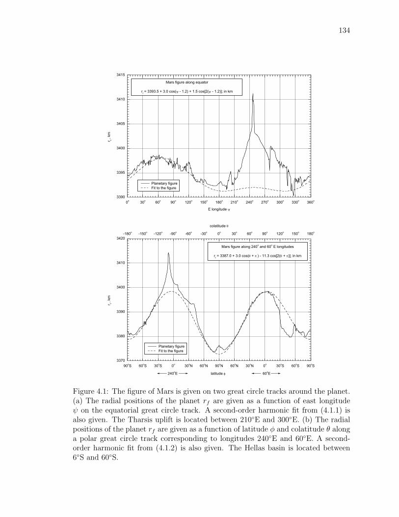
134

0o 30o 60o 90o 120o 150o 180o 210o 240o 270o 300o 330o 360o3390

3395

3400

3405

3410

3415

Mars figure along equator

rf = 3393.5 + 3.0 cos(ψ - 1.2) + 1.5 cos[2(ψ - 1.2)]; in km

r f , k

m

E longitude ψ

Planetary figure Fit to the figure

90oS 60oS 30oS 0o 30oN 60oN 90oN 60oN 30oN 0o 30oS 60oS 90oS3370

3380

3390

3400

3410

3420-180o -150o -120o -90o -60o -30o 0o 30o 60o 90o 120o 150o 180o

Mars figure along 240o and 60o E longitudes

rf = 3387.0 + 3.0 cos(θ + π ) - 11.3 cos[2(θ + π)]; in km

colatitude θ

r f , k

m

240oE latitude φ 60oE

Planetary figure Fit to the figure

Figure 4.1: The figure of Mars is given on two great circle tracks around the planet.(a) The radial positions of the planet rf are given as a function of east longitudeψ on the equatorial great circle track. A second-order harmonic fit from (4.1.1) isalso given. The Tharsis uplift is located between 210E and 300E. (b) The radialpositions of the planet rf are given as a function of latitude φ and colatitude θ alonga polar great circle track corresponding to longitudes 240E and 60E. A second-order harmonic fit from (4.1.2) is also given. The Hellas basin is located between6S and 60S.

135

pansions to the planetary shape given in Figure 4.1. This approach is accurate to

about 1 in 1000 for Mars. For general geodetic considerations for Mars this accu-

racy is not adequate since ellipticity coefficients are known to six significant figures.

However, our purpose is to extract paleogeodetic data, and for this purpose three

significant figure results are adequate. For the equatorial track given in Figure 4.1a

we take the second-order harmonic expansion

rf = af + ∆f cos(ψ + ψ1) +af ef

2cos[2(ψ + ψ2)] , (4.1.1)

where af is the mean equatorial radius, ∆f is the offset of the planetary center of

figure from the Martian center of mass, ef is the equatorial flattening of the figure,

and ψ1 and ψ2 are the phases. We fit the second-order harmonic equation (4.1.1) to

the equatorial planetary shape so as to get a good correspondence to the observed

figure except in the region of the Tharsis construct as shown in Figure 4.1a. We use

the values af = 3393.5 km, ∆f = 3.0 km, and e−1f = 1131.17 (af ef/2 = 1.5 km).

The value of af is less than the actual value (a = 3396.0 km) since we have omitted

the Tharsis construct. Our value of the offset of the planetary figure from its center

of mass ∆f = 3.0 km was previously given by Smith and Zuber, (1996).

Our basic hypothesis is that it is a reasonable approximation to assume that

the topography of the Tharsis region can be attributed to the surface and near

surface emplacements of extrusive and intrusive volcanics. Thus these volcanics

constitute a surface load on the elastic lithosphere. The origin of the volcanics is

the Martian mantle beneath the elastic lithosphere, this mantle behaves in a fluid

like manner. The emplacement mechanism is similar to that responsible for the

Hawaiian-Emperor island-seamount chain on Earth. With mass conservation, the

material in the Tharsis construct requires a reduction of the mean radius of the

planet outside the construct. The net result is a displacement of the center of mass

136

towards the construct.

For the polar great-circle track we use the second-order harmonic relation

rf = rf + ∆f cos(θ + θ1)−af ff

2cos[2(θ + θ2)] , (4.1.2)

where rf is the mean planetary radius for this track, ∆f is the offset of the planetary

center of figure from its center of mass and θ1 and θ2 are the phases. The polar

flattening of the figure is defined by

ff =af − cfaf

, (4.1.3)

where cf is the polar radius of our fit to the planetary figure. Again we fit the second-

order harmonic relation (4.1.2) to the polar figure so that we get a good fit at the

poles and at the antipode of the Tharsis construct as shown in Figure 4.1b. We use

the values rf = 3387.0 km, ∆f = 3.0 km, and af ff/2 = 11.3 km. Taking af =

3393.5 km from above we have f−1f = 150.15. Again our value of rf = 3387.0 km

is less than the mean planetary radius R = 3389.5 km because we have omitted

the Tharsis construct in our fit to the figure. All our results are summarized in

Table 4.1.

To a first approximation, we assume that the Tharsis load is located on the equa-

tor. We also assume that the entire degree-two distortion of the equatorial planetary

figure given by (4.1.1) is caused by the Tharsis load. Because the Tharsis load is

nearly axisymmetric, we assume that a similar distortion of the polar planetary fig-

ure is caused by Tharsis. This approach to the removal of the Tharsis load is similar

to that given by Zuber and Smith, (1997). In accordance with this approximation

we assume that the center of figure, center of mass offsets in (4.1.1) and (4.1.2) are

equal with ∆f = 3.0 km. In order to estimate the polar flattening of the figure of

Mars associated with rotation ffr, we subtract the observed equatorial flattening ef

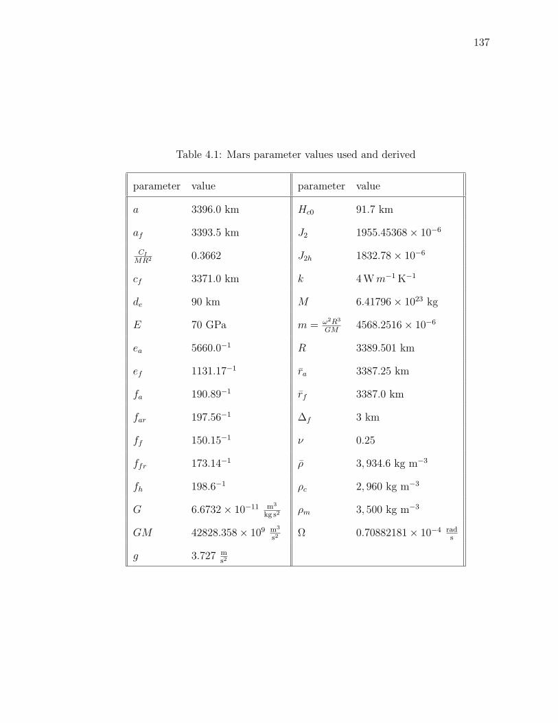
137

Table 4.1: Mars parameter values used and derived

parameter value parameter value

a 3396.0 km Hc0 91.7 km

af 3393.5 km J2 1955.45368× 10−6

CI

MR2 0.3662 J2h 1832.78× 10−6

cf 3371.0 km k 4 Wm−1 K−1

de 90 km M 6.41796× 1023 kg

E 70 GPa m = ω2R3

GM4568.2516× 10−6

ea 5660.0−1 R 3389.501 km

ef 1131.17−1 ra 3387.25 km

fa 190.89−1 rf 3387.0 km

far 197.56−1 ∆f 3 km

ff 150.15−1 ν 0.25

ffr 173.14−1 ρ 3, 934.6 kg m−3

fh 198.6−1 ρc 2, 960 kg m−3

G 6.6732× 10−11 m3

kg s2ρm 3, 500 kg m−3

GM 42828.358× 109 m3

s2Ω 0.70882181× 10−4 rad

s

g 3.727 ms2

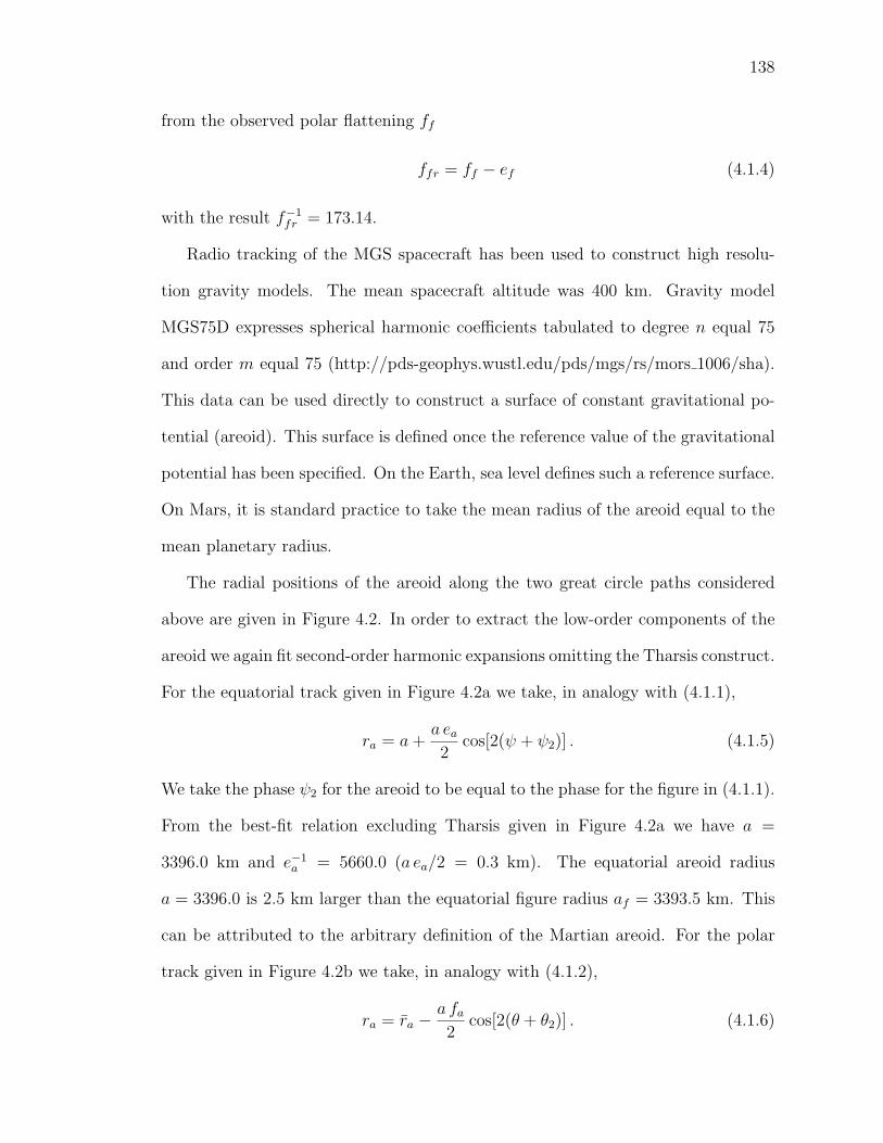
138

from the observed polar flattening ff

ffr = ff − ef (4.1.4)

with the result f−1fr = 173.14.

Radio tracking of the MGS spacecraft has been used to construct high resolu-

tion gravity models. The mean spacecraft altitude was 400 km. Gravity model

MGS75D expresses spherical harmonic coefficients tabulated to degree n equal 75

and order m equal 75 (http://pds-geophys.wustl.edu/pds/mgs/rs/mors 1006/sha).

This data can be used directly to construct a surface of constant gravitational po-

tential (areoid). This surface is defined once the reference value of the gravitational

potential has been specified. On the Earth, sea level defines such a reference surface.

On Mars, it is standard practice to take the mean radius of the areoid equal to the

mean planetary radius.

The radial positions of the areoid along the two great circle paths considered

above are given in Figure 4.2. In order to extract the low-order components of the

areoid we again fit second-order harmonic expansions omitting the Tharsis construct.

For the equatorial track given in Figure 4.2a we take, in analogy with (4.1.1),

ra = a+a ea

2cos[2(ψ + ψ2)] . (4.1.5)

We take the phase ψ2 for the areoid to be equal to the phase for the figure in (4.1.1).

From the best-fit relation excluding Tharsis given in Figure 4.2a we have a =

3396.0 km and e−1a = 5660.0 (a ea/2 = 0.3 km). The equatorial areoid radius

a = 3396.0 is 2.5 km larger than the equatorial figure radius af = 3393.5 km. This

can be attributed to the arbitrary definition of the Martian areoid. For the polar

track given in Figure 4.2b we take, in analogy with (4.1.2),

ra = ra −a fa

2cos[2(θ + θ2)] . (4.1.6)

139

From our best-fit relation we have ra = 3387.25 km and a fa/2 = 8.895 km. Taking

a = 3396.0 km from above gives f−1a = 190.89. The mean polar areoid radius

ra = 3387.25 km is essentially equal to the mean polar figure radius rf = 3387.0 km.

We again assume that, to a first approximation, the degree-two distortion of

the equatorial areoid given by (4.1.5) can be attributed to the Tharsis load and

that a similar distortion occurs to the polar areoid. In order to estimate the polar

flattening of the areoid of Mars associated with rotation far we subtract the observed

equatorial flattening ea from the observed polar flattening fa

far = fa − ea (4.1.7)

with the result f−1ar = 197.56. The polar flattening of the figure f−1

fr = 173.14 is

considerably larger than the polar flattening of the areoid f−1ar = 197.56.

Using Darwin-Radau relation (1.2.3) defined in Chapter 1 we can calculate the

hydrostatic flattening fh. For Mars, m = 4568.2516× 10−6 and we take CI/MR2 =

0.3662± 0.0017 (Folkner et al., 1997). With these values the hydrostatic flattening

for Mars is f−1h = 198.6. This value is relatively close to the flattening of the areoid

f−1ar = 197.56 but is considerably less than the flattening of the figure f−1

fr = 173.14.

A detailed discussion of the hydrostatic flattening of Mars has been given by Sleep

and Phillips , (1985).

The usual explanation for the paleoflattening of the figure of a planetary body

is tidal despinning. The flattening of the figure was caused by a higher rotational

velocity in the past. As the rotation slowed due to tidal interactions the membrane

stresses preserved the fossil ellipticity (flattening). This mechanism was applied

to explain both the fossil figure and the global fracture pattern on Mercury by

Melosh, (1977) and by Melosh and Dzurisin, (1978). This mechanism has also been

used to explain a fossil flattening on the moon (Jeffreys, 1976; Willemann and

140

0o 30o 60o 90o 120o 150o 180o 210o 240o 270o 300o 330o 360o3395

3396

3397

3398

Mars areoid radius along equator

ra = 3396.0 + 3.0 cos[2(ψ - 1.2)]; in km

r a , k

m

E longitude ψ

Areoid radius Fit to the areoid radius

90oS 60oS 30oS 0o 30oN 60oN 90oN 60oN 30oN 0o 30oS 60oS 90oS3375

3380

3385

3390

3395

3400

3405-180o -150o -120o -90o -60o -30o 0o 30o 60o 90o 120o 150o 180o

Mars areoid radius along 240o and 60o E longitudes

ra = 3387.25 + 8.895 cos[2(θ + π)]; in km

colatitude θ

r a , k

m

240oE latitude φ 60oE

Areoid radius Fit to the areoid radius

Figure 4.2: The areoid of Mars is given on two great circle tracks around the planet.(a) The radial positions of the areoid ra are given as a function of east longitude ψon the equatorial great circle track. A second-order harmonic fit from (4.1.4) is alsogiven. (b) The radial positions of the areoid ra are given as a function of latitudeφ and colatitude θ on a polar great-circle track corresponding to longitudes 240Eand 60E. A second-order harmonic fit from (4.1.5) is also given.

141

Turcotte, 1981). To obtain the observed flattening of figure for Mars, f−1fr = 173.14,

from (1.2.3) we require thatm = 5224.0×10−6. This would require a fossil rotational

velocity seven percent greater than the present value.

The estimate given above assumes that the fossil flattening is completely sup-

ported by the elastic lithosphere. In fact, some relaxation is expected so that the

required fossil rotational velocity would be somewhat larger than the seven percent

given above.

Since Mars does not have a large moon and is considerably further from the

Sun than the Earth, tidal despinning may not be a plausible explanation for the

high fossil rotational velocity. An alternative explanation would be the transfer of

angular momentum in a massive impact, possibly the impact responsible for the

formation of the Hellas basin. Whatever the cause, a change in rotational velocity

appears to be necessary to explain the present ellipticity of the planetary figure.

To the same quadratic approximation used in (1.2.3) , the coefficient J2h is given

by

J2h =2

3fh −

1

3m (4.1.8)

and using the values of fh and m above we have J2h = 1832.78 × 10−6. The value

of J2 obtained from the gravity field of Mars is J2 = 1955.45368 × 10−6. Thus

there is clearly a large non-hydrostatic component to the present gravity field. A

large fraction of the non-hydrostatic component of the degree 2 gravity field can

be attributed to the mass of the Tharsis construct (Reasenberg, 1977; Kaula, 1979;

Bills, 1989; Zuber and Smith, 1997; Bills and James, 1999) as discussed above.

In the hydrostatic approximation the surface of a planetary body coincides with

its areoid. In the analysis given above we attributed the degree two distortion of

the equatorial figure and areoid to the loading of the Tharsis construct. Assuming

142

that the Tharsis load is axisymmetric and is centered on the equator we assumed

that the degree two distortions of the polar figure and areoid due to this load are

equal to the distortions of the equatorial figure and areoid. With these assumptions

we found that the polar flattening of the figure is f−1fr = 173.14 and of the areoid is

f−1ar = 197.56. These compare with the predicted hydrostatic flattening f−1

h = 198.6.

It is general practice to define topography to be the elevation difference between

the radial position of the surface and the radial position of the equipotential surface

(areoid). For the Earth this definition is the elevation above sea level, clearly a

reasonable definition. For Mars, this definition gives the “load” on the lithosphere

due to the topography. Defining topography in this manner, the topography along

the equatorial and polar great circles tracks considered in Figure 4.1 are given in

Figure 4.3. The topography is the difference between the figure given in Figure 4.1

and the areoid given in Figure 4.2. Clearly there are significant degree 2 distortions

in both the equatorial and polar topography. These distortions can be attributed

to the rigidity of the elastic lithosphere on Mars. The distortion of the equatorial

topography can be attributed to the support of the Tharsis construct by elastic

shell (membrane) stresses. For the polar topography, both this effect and the fossil

flattening of the figure contribute to the degree 2 distortion of the topography.

Thus topography defined as the elevation difference between the radial position of

the surface and the radial position of the areoid is relatively meaningless. As an

alternative definition of topography, we consider the elevation difference between

the radial position of the Martian surface and the reference figure of the planet as

given in Figure 4.1. The topography determined in this manner along the equatorial

and polar great circle tracks considered in Figure 4.1 are also given in Figure 4.3.

We will use this topography in the correlation between areoid anomaly height and

143

topography considered in the next section.

4.2 Hellas Analysis

A major topographic feature on Mars is the Hellas impact basin. The topography

of the basin is evident on the 60E polar track given in Figure 4.3b. This basin is

located between 6S and 59S and has a maximum depth of about 9 km. Most impact

basins on the moon and some on Mars have gravity highs known as “mascons”.

Mascons are associated with “buried” loads which can contribute to the negative

topography of the basin. The Hellas basin does not have a significant mascon

(positive gravity anomaly). There is also no evidence that the negative load of the

excavated basin is supported by bending or shell stresses in the elastic lithosphere.

It appears that the Hellas basin is fully compensated, to a good approximation.

For fully compensated topography, the topography at a point is directly related

to the geoid (areoid) anomaly at that point. Mechanisms of compensation include

Airy, Pratt, and thermal. For the Hellas basin we hypothesize that the compensation

is due to variations in crustal thickness (Airy compensation). For a constant density

crust, the areoid anomaly ∆N at a point is related to the topography at that point

h by the relation (Turcotte and Schubert, 1982, Eq. 5–148)

∆N =2π ρcG

g

[hHc0 +

1

2

(ρm

ρm − ρc

)h2

], (4.2.1)

where G is the gravitational constant, g the surface gravity, ρm mantle density, ρc

crustal density, and Hc0 is the reference (zero elevation) crustal thickness.

In obtaining geoid (areoid) height-topography correlations for a geological fea-

ture, it is standard practice to use data along a single track (Sandwell and MacKen-

zie, 1989). We consider topography and areoid data for Hellas along the north-south

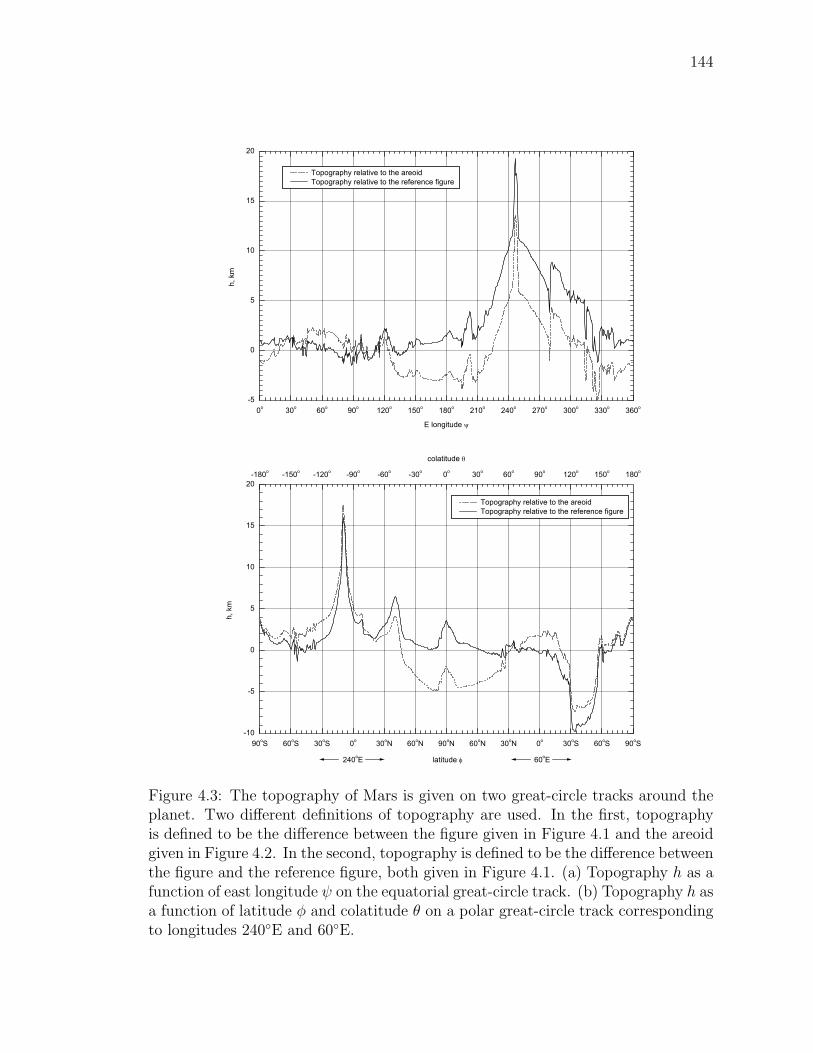
144

0o 30o 60o 90o 120o 150o 180o 210o 240o 270o 300o 330o 360o-5

0

5

10

15

20

h, k

m

E longitude ψ

Topography relative to the areoid Topography relative to the reference figure

90oS 60oS 30oS 0o 30oN 60oN 90oN 60oN 30oN 0o 30oS 60oS 90oS-10

-5

0

5

10

15

20-180o -150o -120o -90o -60o -30o 0o 30o 60o 90o 120o 150o 180o

colatitude θ

h, k

m

240oE latitude φ 60oE

Topography relative to the areoid Topography relative to the reference figure

Figure 4.3: The topography of Mars is given on two great-circle tracks around theplanet. Two different definitions of topography are used. In the first, topographyis defined to be the difference between the figure given in Figure 4.1 and the areoidgiven in Figure 4.2. In the second, topography is defined to be the difference betweenthe figure and the reference figure, both given in Figure 4.1. (a) Topography h as afunction of east longitude ψ on the equatorial great-circle track. (b) Topography h asa function of latitude φ and colatitude θ on a polar great-circle track correspondingto longitudes 240E and 60E.

145

great-circle track at 60E longitude illustrated in Figures 4.3b and 4.2b. We assume

that the topography is the difference between the figure and the fit to the figure

as given in Figure 4.3b. This topography is given in Figure 4.4a. We obtain the

corresponding areoid anomaly ∆N by taking the difference between the areoid and

the fit to the areoid as given in Figure 4.2b. The result is given in Figure 4.4b. The

data in both Figures 4.4a and 4.4b are plotted at 1 (59.2 km) intervals (1S, 2S,

..., 60S).

The areoid anomaly at each point along the track from Figure 4.4b is plotted

against the residual topography at that point from Figure 4.4a at 1 intervals along

the track in Figure 4.5. The best-fit quadratic relation (∆N = c0 + c1h + c2h2) is

also given in the figure. The quadratic fit was chosen because it corresponds to the

quadratic dependence given in (4.2.1).

In order to make a direct comparison with the isostatic prediction (4.2.1) we

assume g = 3.727 m s−2 and ρm = 3, 500 kg m−3 (Sohl and Spohn, 1997). From

the coefficient of the quadratic term (c2 = 1.08 m km−2) in Figure 4.5 we obtain

ρc = 2, 960 kg m−3. This is a very reasonable value for the mean crustal density

of an iron-rich planet. Using this value for ρc in the linear term, the coefficient of

the linear term (c1 = 30.56 m km−1) requires that the reference crustal thickness

be Hc0 = 91.7 km. It should be noted that the coefficient of the linear term is also

known as the geoid (areoid)-topography ratio (GTR).

In the correlation given in Figure 4.5 we find that ∆N = 133.9 m, when h = 0.

This is not surprising since our topography is referenced to a paleofigure flattening

while the areoid is referenced to the present areoid flattening. Based on the scatter

of the data for the Hellas basin given in Figure 4.5 we conclude that the reference

(zero elevation) crustal thickness on Mars is Hc0 = 90 ± 10 km and that the mean

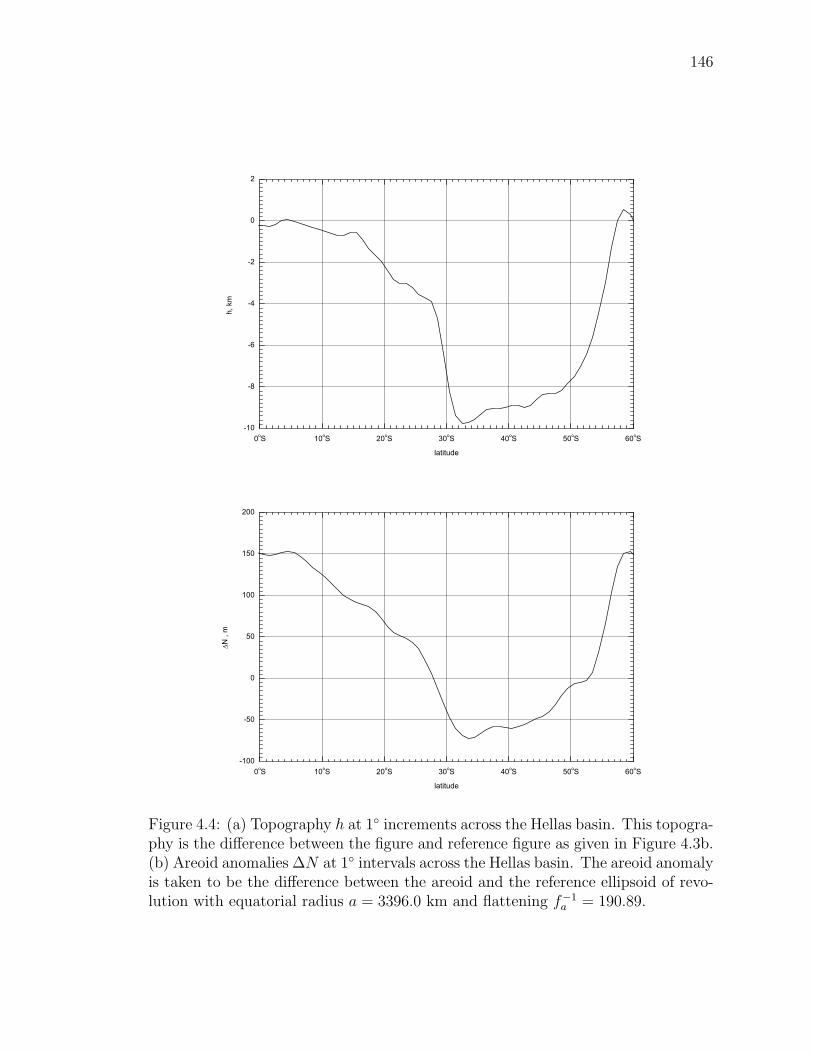
146

0oS 10oS 20oS 30oS 40oS 50oS 60oS-10

-8

-6

-4

-2

0

2

h, k

m

latitude

0oS 10oS 20oS 30oS 40oS 50oS 60oS-100

-50

0

50

100

150

200

∆N ,

m

latitude

Figure 4.4: (a) Topography h at 1 increments across the Hellas basin. This topogra-phy is the difference between the figure and reference figure as given in Figure 4.3b.(b) Areoid anomalies ∆N at 1 intervals across the Hellas basin. The areoid anomalyis taken to be the difference between the areoid and the reference ellipsoid of revo-lution with equatorial radius a = 3396.0 km and flattening f−1

a = 190.89.

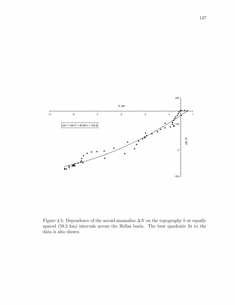
147

∆N = 1.08 h2 + 30.56 h + 133.9

-100

0

100

200

-11 -9 -7 -5 -3 -1 1

h, km

∆N, m

Figure 4.5: Dependence of the areoid anomalies ∆N on the topography h at equallyspaced (59.2 km) intervals across the Hellas basin. The best quadratic fit to thedata is also shown.

148

crustal density is ρc = 2, 960 ± 50 kg m−3. Using the isostatic assumption, the

thickness of the crust at the deepest part of the basin (h = −9 km) is Hc = 33 km.

At this point the Moho is elevated 48 km above its reference value.

In the analysis given above we have implicitly assumed that the crustal density

is constant. However, the massive impact responsible for the excavation of the basin

may have induced substantial melting of both crustal and mantle rock. This melting

episode could have produced crustal rock with a larger density than average Martian

crust. We believe the excellent correlation with the constant density theory across

the entire basin illustrated in Figure 4.5 supports our hypothesis of a nearly constant

crustal density.

There is also the question of thermal compensation. Significant elevation changes

are associated with changes in the thickness of the thermal lithosphere. At the time

of the impact it is likely that the lithosphere was thinned in the vicinity of the Hellas

basin (consistent with isostasy). But subsequently the lithosphere would thicken by

conduction so that there would be no thermally induced topography today. Again

this conclusion is substantiated by the correlations given in Figure 4.5. Thermal

compensation would result in significant deviations from the Airy results given in

this figure.

A variety of estimates have been made for the crustal thickness on Mars. Sjogren

and Wimberley, (1981) also correlated gravity with topography across the Hellas

basin and estimated that the depth of compensation is between 100 and 160 km.

With Airy compensation this would also be the crustal thickness Hc. Bills and

Ferrari, (1978) obtained a crustal thickness in the range Hc = 24 – 32 km from low-

order gravity and topography harmonics assuming zero crustal thickness beneath

Hellas. Sohl and Spohn, (1997) estimated a crustal thickness Hc = 100 – 250 km and

149

Norman, (1999) argues that the thickness is less than 45 km. Zuber et al., (2000)

give a lower bound on crustal thickness of Hc = 50 km and argue that thermal

considerations limit the crustal thickness to 100 km. Nimmo and Stevenson, (2001)

support these values. Nimmo, (2001) also used geoid-topography ratios to obtain the

crustal thickness across the crustal dichotomy, his preferred values are 50 – 75 km.

Kucinskas et al., (2001) used spatial GTR modeling and MGS data to obtain a

mean reference crustal thickness, for regions where Airy isostasy is a viable support

mechanism, of approximately 100 km.

4.3 Compensation

In carrying out the analysis of the Hellas impact basin we assumed that this to-

pographic feature is locally compensated. However, much of the topography on

Mars is only partially compensated. If h is the height of the topography and w is

the downward deflection of the lithosphere caused by the topography, for locally

compensated topography we have

w =ρc h

ρm − ρc

. (4.3.1)

For partially compensated topography we have

w = Cρc h

ρm − ρc

, (4.3.2)

where C is the degree of compensation (0 ≤ C ≤ 1). If there is no deflection of

the lithosphere due to the weight of the topography, there is no compensation and

C = 0.

With the assumption of partial Airy compensation, the surface free-air gravity

anomaly ∆gfa is made up of two parts

∆gfa = ∆gt + ∆gm , (4.3.3)

150

where ∆gt is the gravity anomaly due to the topography and ∆gm is the gravity

anomaly due to the deflection of the Moho. With the Bougher assumption, the

gravity anomaly due to the topography is given by

∆gt = 2π ρcGh . (4.3.4)

The gravity anomaly due to the deflection of the Moho is given by (Turcotte and

Schubert, 1982, Eq. 5–123)

∆gm = −2π(ρm − ρc)Gw exp(−2πHc0

λn

), (4.3.5)

where λn is the wavelength of the topography being considered. The exponential

term is required since there is a decay in the gravity signal from the Moho if the

mean depth of the Moho Hc is not small compared with the wavelength of the

topography on the Moho λn. We define the gravity-topography admittance A to

be the ratio of the free-air gravity anomaly ∆gfa to the topography h. Combining

Eqs. (4.3.2), (4.3.3), (4.3.4), and (4.3.5) we obtain

A =∆gfa

h= 2πρcG

[1− Cn exp

(−2πHc0

λn

)]. (4.3.6)

The gravity-topography admittance, A = ∆gfa/h, is specified when the degree of

compensation Cn is specified.

For a relatively small planetary body like Mars, the degree of compensation of

topographic loads is controlled by both bending and membrane (shell) stresses in the

elastic lithosphere. Turcotte et al., (1981) have solved this problem and they found

that the degree of compensation Cn for a topographic load of spherical harmonic

degree n is given by

Cn =

1− 3ρm

(2n+ 1)ρ

σ[m3 − 4m2

]+ τ [m− 2]

m− 1 + ν + 1− 3ρm

(2n+ 1)ρ

, (4.3.7)

151

with m = n(n+ 1), ρ the mean planetary density, ν Poisson’s ratio, σ the bending

rigidity

σ =τ

12(1− ν2)

(de

R

)2

, (4.3.8)

and τ the shell rigidity

τ =E de

R2 g (ρm − ρc), (4.3.9)

with E Young’s modulus and de the elastic lithosphere thickness. This is the thick-

ness of the elastic lithosphere at the time the load was applied. If the elastic litho-

sphere subsequently thickened due to a reduction in the near-surface thermal gra-

dient, the deformation due to the load is “frozen-in”.

It should be emphasized that the analysis given above assumes that the loading of

the lithosphere is from above. The loads of the additional crustal rocks at the surface

are supported by the elastic lithosphere leading to positive gravity anomalies. If

additional crustal rocks are emplaced at depth without disturbing the upper crustal

rocks, they constitute a buried load. Crustal rocks emplaced at the Moho would

lead to a downward displacement of the Moho and upward load resulting in negative

gravity anomalies. It has been argued that it is necessary to consider these buried

loads when considering correlations of topography and gravity on Earth (Forsyth,

1985; Bechtel et al., 1990). Since we see strong positive correlations of gravity with

topography we will assume that the entire loading on Mars is from above. However,

we recognize that partial subsurface loading can increase the thickness of the elastic

lithosphere relative to the values we have obtained.

We will utilize the spherical harmonic coefficients of the planetary figure and

areoid (gravity potential) to study the compensation of Martian topography on a

152

global basis. The variance of the planetary figure spectra for degree n is defined as

Vfn = R2n∑

m=0

(C2

fnm + S2fnm

)(4.3.10)

and for areoid spectra the variance is

Van = R2n∑

m=0

(C2

anm + S2anm

), (4.3.11)

where the Cnm and Snm are the spherical harmonic coefficients (Turcotte, 1987).

The power spectral density Sf of the figure is defined according to

Sf (kn) = 2π RVfn (4.3.12)

with a similar relation for the areoid. The wave number kn and wavelength λn are

defined by

kn =1

λn

=n

2π R. (4.3.13)

Using the degree n equal 90 and order m equal 90 spherical harmonic expansion

of the MGS planetary figure data (http://ltpwww.gsfc.nasa.gov/tharsis/mola.html),

the dependence of the power spectral density coefficients of the planetary figure

Sf (kn) on degree n and wave number kn is given in Figure 4.6.

The definition of a self-affine fractal is that the power spectral density has a

power-law dependence on wave number (frequency) and wavelength of the form

(Turcotte, 1997, Eq. 7–41)

S(kn) ∼ k−βn ∼ λβ

n . (4.3.14)

It is seen that the Martian planetary figure correlates well with this relation taking

β = 1.9. A Brownian motion has β = 2.0. Many authors have previously noted

that planetary topography (the figure) also has β ≈ 2.0 (Turcotte, 1987). Smith

et al., (2001) have also shown that the power spectrum of Martian topography

satisfies (4.3.14), they found β = 1.9346.

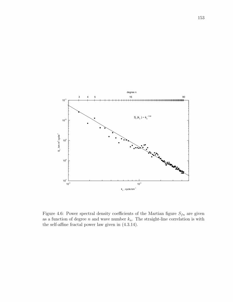
153

10-4 10-3107

108

109

1010

101116 90543

degree n

Sf (kn ) ~ kn-1.92

S f , k

m m

2 cyc

le-1

kn , cycle km-1

Figure 4.6: Power spectral density coefficients of the Martian figure Sfn are givenas a function of degree n and wave number kn. The straight-line correlation is withthe self-affine fractal power law given in (4.3.14).

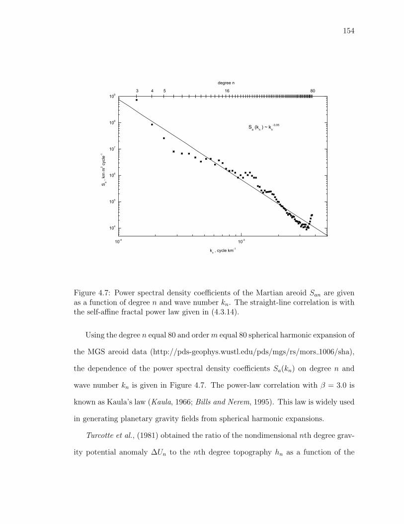
154

10-4 10-3

104

105

106

107

108

10916 80543

Sa (kn ) ~ kn-3.05

degree n

S a , k

m m

2 cyc

le-1

kn , cycle km-1

Figure 4.7: Power spectral density coefficients of the Martian areoid San are givenas a function of degree n and wave number kn. The straight-line correlation is withthe self-affine fractal power law given in (4.3.14).

Using the degree n equal 80 and orderm equal 80 spherical harmonic expansion of

the MGS areoid data (http://pds-geophys.wustl.edu/pds/mgs/rs/mors 1006/sha),

the dependence of the power spectral density coefficients Sa(kn) on degree n and

wave number kn is given in Figure 4.7. The power-law correlation with β = 3.0 is

known as Kaula’s law (Kaula, 1966; Bills and Nerem, 1995). This law is widely used

in generating planetary gravity fields from spherical harmonic expansions.

Turcotte et al., (1981) obtained the ratio of the nondimensional nth degree grav-

ity potential anomaly ∆Un to the nth degree topography hn as a function of the

155

degree of compensation Cn with the result

∆Un

hn

=3ρc

(2n+ 1)ρ

[1− Cn

(1− Hc0

R

)n+2]. (4.3.15)

The nth degree nondimensional gravity potential anomaly ∆Un is defined by

∆Un =R

GM

n∑m=0

(C2

anm + S2anm

) 12 (4.3.16)

and the nth degree nondimensional topography hn is defined by

hn =1

R

n∑m=0

(C2

fnm + S2fnm

) 12 . (4.3.17)

The ratios of these coefficients ∆Un/hn for Mars are given as a function of n to

degree 80 in Figure 4.8.

Taking ρc = 2, 960 kg m−3, ρm = 3, 500 kg m−3, g = 3.727 m s−2, R =

3, 389.5 km, E = 70 GPa, ν = 0.25, ρ = 3, 934.6 kg m−3, and Hc0 = 91.7 km

we determine ∆Un/hn from (4.3.7), (4.3.8), (4.3.9), and (4.3.15) for five values of

the thickness of the elastic lithosphere 0 ≤ de ≤ 200 km. These results are given in

Figure 4.8. This data is a relatively weak constraint on the globally averaged thick-

ness of the elastic lithosphere de, we conclude based on Figure 4.8 that a reasonable

range of values is de = 100 ± 50 km. In the next section we obtain an improved

constraint utilizing wavelet transforms.

4.4 Wavelet Analysis

In order to obtain gravity-topography admittances for Mars we will utilize the

wavelet transform. We will consider the 1D tracks of topography and gravity along

the equatorial and polar 60E – 240E great circles as “time series”. The gravity-

topography admittance of these 1D tracks can be obtained using fast Fourier trans-

forms. However, we will utilize the wavelet transform instead in order to obtain

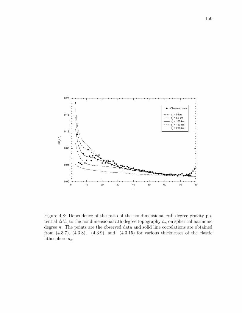
156

0 10 20 30 40 50 60 70 800.00

0.04

0.08

0.12

0.16

0.20

∆Un /

hn

n

Observed data

de = 0 km de = 50 km de = 100 km de = 150 km de = 200 km

Figure 4.8: Dependence of the ratio of the nondimensional nth degree gravity po-tential ∆Un to the nondimensional nth degree topography hn on spherical harmonicdegree n. The points are the observed data and solid line correlations are obtainedfrom (4.3.7), (4.3.8), (4.3.9), and (4.3.15) for various thicknesses of the elasticlithosphere de.

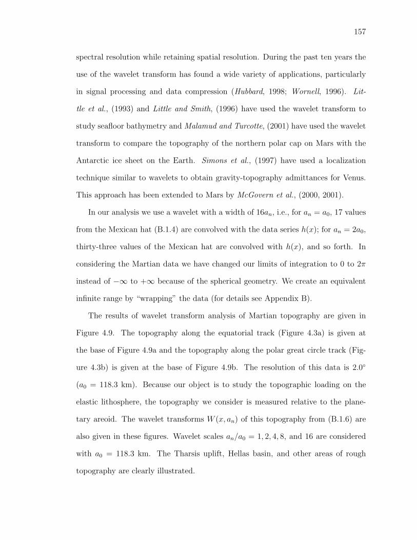
157

spectral resolution while retaining spatial resolution. During the past ten years the

use of the wavelet transform has found a wide variety of applications, particularly

in signal processing and data compression (Hubbard, 1998; Wornell, 1996). Lit-

tle et al., (1993) and Little and Smith, (1996) have used the wavelet transform to

study seafloor bathymetry and Malamud and Turcotte, (2001) have used the wavelet

transform to compare the topography of the northern polar cap on Mars with the

Antarctic ice sheet on the Earth. Simons et al., (1997) have used a localization

technique similar to wavelets to obtain gravity-topography admittances for Venus.

This approach has been extended to Mars by McGovern et al., (2000, 2001).

In our analysis we use a wavelet with a width of 16an, i.e., for an = a0, 17 values

from the Mexican hat (B.1.4) are convolved with the data series h(x); for an = 2a0,

thirty-three values of the Mexican hat are convolved with h(x), and so forth. In

considering the Martian data we have changed our limits of integration to 0 to 2π

instead of −∞ to +∞ because of the spherical geometry. We create an equivalent

infinite range by “wrapping” the data (for details see Appendix B).

The results of wavelet transform analysis of Martian topography are given in

Figure 4.9. The topography along the equatorial track (Figure 4.3a) is given at

the base of Figure 4.9a and the topography along the polar great circle track (Fig-

ure 4.3b) is given at the base of Figure 4.9b. The resolution of this data is 2.0

(a0 = 118.3 km). Because our object is to study the topographic loading on the

elastic lithosphere, the topography we consider is measured relative to the plane-

tary areoid. The wavelet transforms W (x, an) of this topography from (B.1.6) are

also given in these figures. Wavelet scales an/a0 = 1, 2, 4, 8, and 16 are considered

with a0 = 118.3 km. The Tharsis uplift, Hellas basin, and other areas of rough

topography are clearly illustrated.

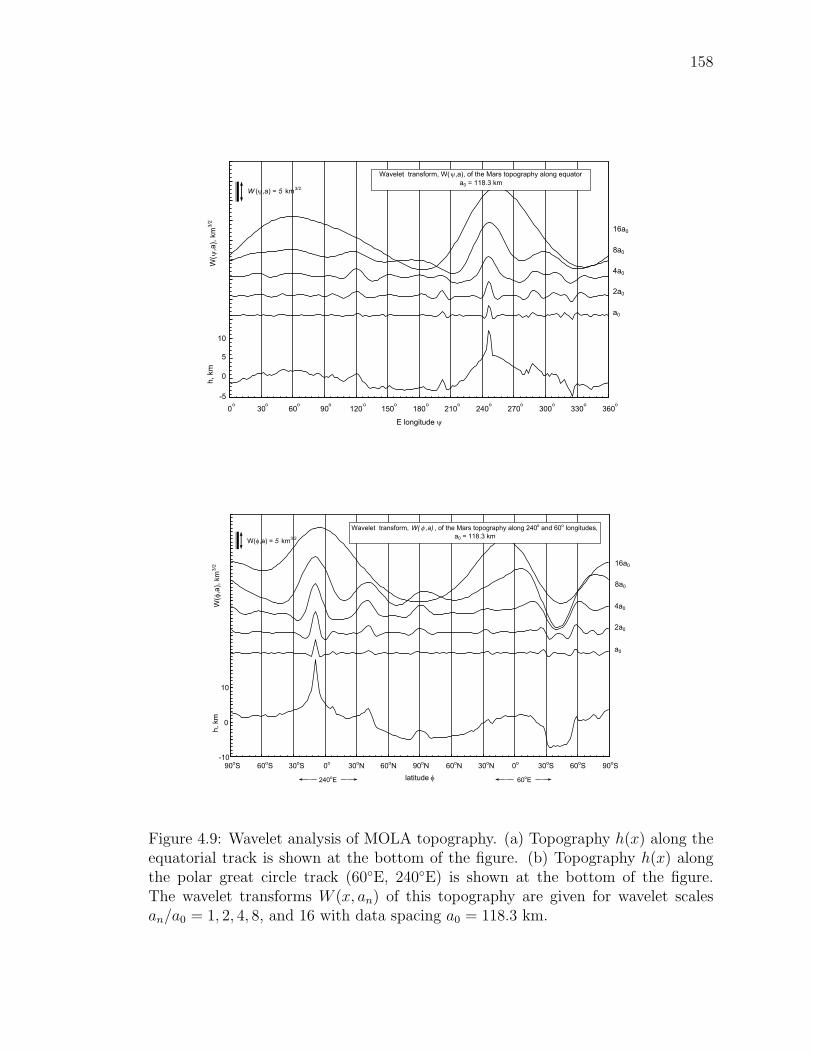
158

0 30 60 90 120 150 180 210 240 270 300 330 360

E longitude ψ

Wavelet transform, W(ψ,a), of the Mars topography along equator a0 = 118.3 km

a0

2a0

4a0

8a0

16a0

o o o o oo o o o o o o o

0

5

-5

h, k

mW

( ψ,a

), km

3/2

10

W (ψ,a) = 5 km3/2

latitude φ

Wavelet transform, W( φ ,a) , of the Mars topography along 240o and 60o longitudes, a0 = 118.3 km

a0

2a0

4a0

8a0

16a0

0

10

-10

h, k

mW

( φ,a

), km

3/2

90oS 60oS 30oS 0o 30oN 60oN 90oN 60oN 30oN 0o 30oS 60oS 90oS

240oE 60oE

W(φ,a) = 5 km3/2

Figure 4.9: Wavelet analysis of MOLA topography. (a) Topography h(x) along theequatorial track is shown at the bottom of the figure. (b) Topography h(x) alongthe polar great circle track (60E, 240E) is shown at the bottom of the figure.The wavelet transforms W (x, an) of this topography are given for wavelet scalesan/a0 = 1, 2, 4, 8, and 16 with data spacing a0 = 118.3 km.

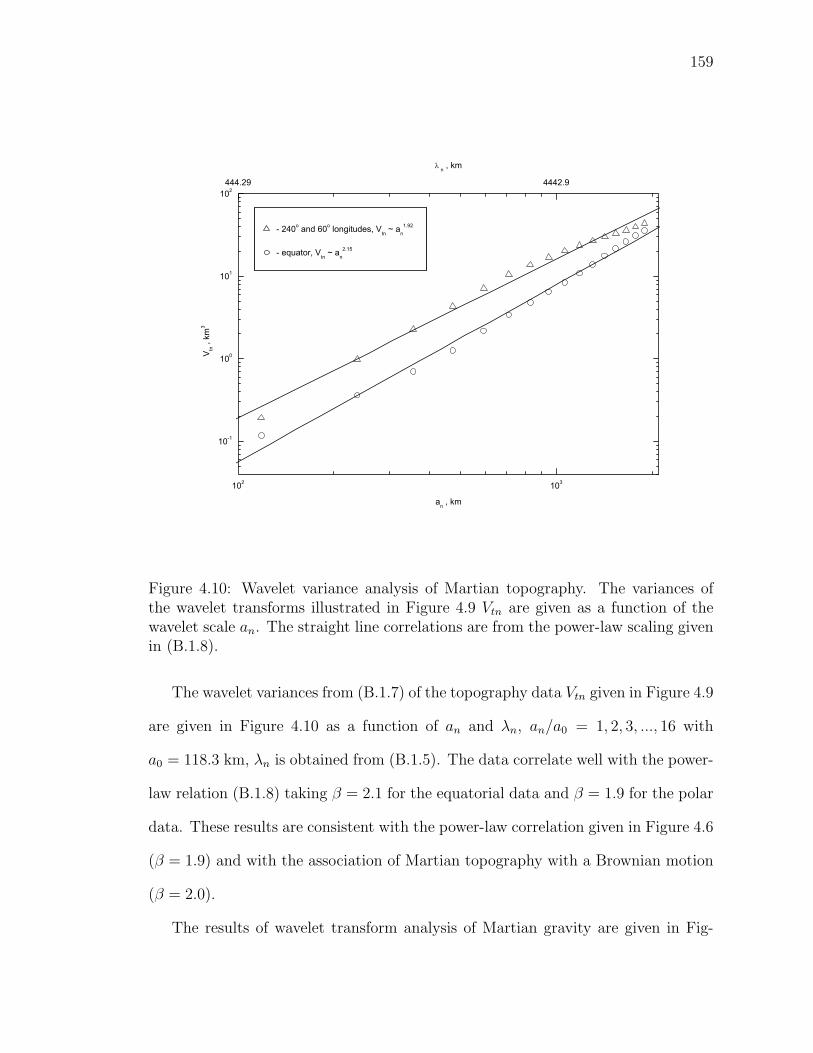
159

102 103

10-1

100

101

102444.29 4442.9

λ n , km

V tn ,

km3

an , km

- 240o and 60o longitudes, Vtn ~ an1.92

- equator, Vtn ~ an2.15

Figure 4.10: Wavelet variance analysis of Martian topography. The variances ofthe wavelet transforms illustrated in Figure 4.9 Vtn are given as a function of thewavelet scale an. The straight line correlations are from the power-law scaling givenin (B.1.8).

The wavelet variances from (B.1.7) of the topography data Vtn given in Figure 4.9

are given in Figure 4.10 as a function of an and λn, an/a0 = 1, 2, 3, ..., 16 with

a0 = 118.3 km, λn is obtained from (B.1.5). The data correlate well with the power-

law relation (B.1.8) taking β = 2.1 for the equatorial data and β = 1.9 for the polar

data. These results are consistent with the power-law correlation given in Figure 4.6

(β = 1.9) and with the association of Martian topography with a Brownian motion

(β = 2.0).

The results of wavelet transform analysis of Martian gravity are given in Fig-

160

ure 4.11. The gravity data was obtained from the same spherical harmonic set of

coefficients used to determine the areoid. The gravity along the equatorial track is

given at the base of Figure 4.11a and the gravity along the polar great circle track is

given at the base of Figure 4.11b. The resolution of this data is 2.0 (a0 = 118.3 km).

The wavelet transforms (B.1.6) of these gravity profiles are also given. Wavelet scales

an/a0 = 1, 2, 4, 8, and 16 are considered with a0 = 118.3 km.

Since the wavelet transform data in Figures 4.9 and 4.11 give both spatial and

wavelength information, a comparison of these figures can be used to determine

whether gravity anomalies correlate with topography. In most cases there is a strong

positive correlation. Also, a large fraction of the signal in both data sets is associated

with the Tharsis region.

The wavelet variances from (B.1.7) of the gravity data Vgn given in Figure 4.11 are

given in Figure 4.12 as a function of wavelet scale an and wavelength λn, an/a0 =

1, 2, ..., 16 with a0 = 118.3 km, λn is obtained from (B.1.5). The data correlate

moderately well with the power-law relation (B.1.8) taking β = 1.2 for the equatorial

data and β = 1.1 for the polar data. A power law β = 1.0 for the gravity data is

equivalent to a power law β = 3.0 for the Martian areoid data as found in Figure 4.7

(Kaula’s law). This is because the variance of the gravity at degree n, Vgn, is related

to the variance of areoid at degree n, Van, by Vgn ∼ n2Van (Jeffreys, 1976).

The gravity-topography admittances of a planetary lithosphere An have been

given as a function of the degree of compensation Cn in (4.3.6). The degree of

compensation Cn at spherical harmonic degree n has been given in (4.3.7)–(4.3.9).

In terms of our wavelet spectral analysis it is appropriate to define the gravity-

topography admittance An as

An =(Vgn

Vtn

) 12

. (4.4.1)

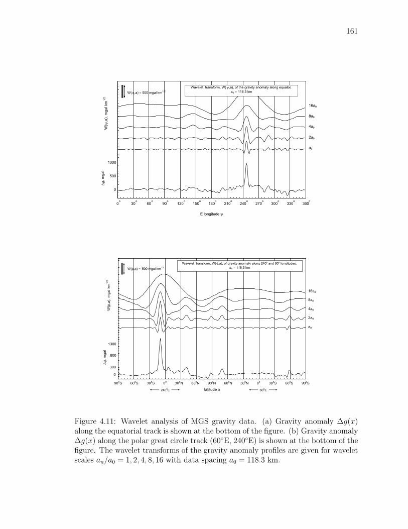
161

0 30 60 90 120 150 180 210 240 270 300 330 360

E longitude ψ

Wavelet transform, W(ψ,a), of the gravity anomaly along equator, a0 = 118.3 km

a0

2a0

4a0

8a0

16a0

0

500

∆g, m

gal

1000

W( ψ

,a),

mga

l km

1/2

o o o o o o o o ooooo

W(ψ,a) = 500 mgal km1/2

latitude φ

Wavelet transform, W(φ,a), of gravity anomaly along 240o and 60o longitudes, a0 = 118.3 km

a0

2a0

4a0

8a0

16a0

0

300

800

∆g, m

gal

90oS 60oS 30oS 0o 30oN 60oN 90oN 60oN 30oN 0o 30oS 60oS 90oS

240oE 60oE

1300

W( φ, a

), m

gal k

m1/

2

W(φ,a) = 500 mgal km1/2

Figure 4.11: Wavelet analysis of MGS gravity data. (a) Gravity anomaly ∆g(x)along the equatorial track is shown at the bottom of the figure. (b) Gravity anomaly∆g(x) along the polar great circle track (60E, 240E) is shown at the bottom of thefigure. The wavelet transforms of the gravity anomaly profiles are given for waveletscales an/a0 = 1, 2, 4, 8, 16 with data spacing a0 = 118.3 km.

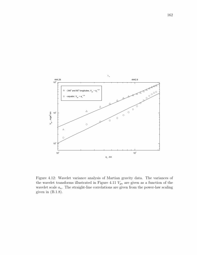
162

102 103

103

104

105444.29 4442.9

λ n

V gn ,

mga

l2 km

an , km

- 240o and 60o longitudes, Vgn ~ an1.07

- equator, Vgn ~ an1.24

Figure 4.12: Wavelet variance analysis of Martian gravity data. The variances ofthe wavelet transforms illustrated in Figure 4.11 Vgn are given as a function of thewavelet scale an. The straight-line correlations are given from the power-law scalinggiven in (B.1.8).

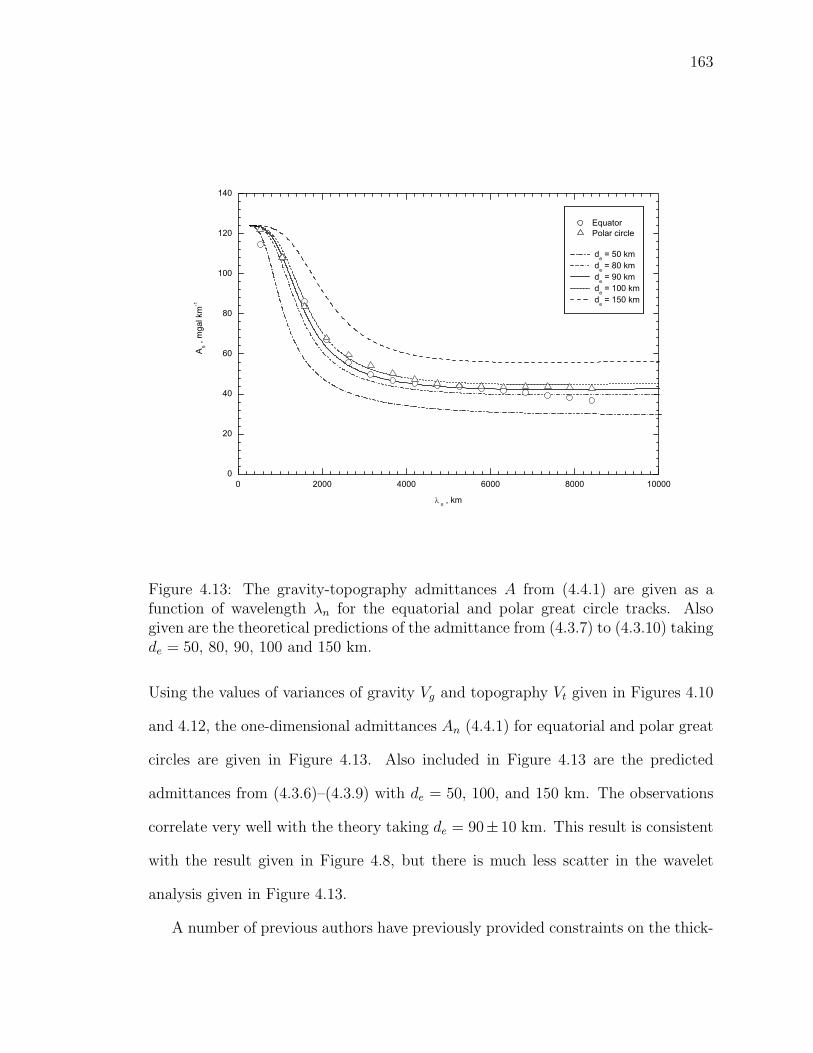
163

0 2000 4000 6000 8000 100000

20

40

60

80

100

120

140

A n ,

mga

l km

-1

λ n , km

Equator Polar circle

de = 50 km de = 80 km de = 90 km de = 100 km de = 150 km

Figure 4.13: The gravity-topography admittances A from (4.4.1) are given as afunction of wavelength λn for the equatorial and polar great circle tracks. Alsogiven are the theoretical predictions of the admittance from (4.3.7) to (4.3.10) takingde = 50, 80, 90, 100 and 150 km.

Using the values of variances of gravity Vg and topography Vt given in Figures 4.10

and 4.12, the one-dimensional admittances An (4.4.1) for equatorial and polar great

circles are given in Figure 4.13. Also included in Figure 4.13 are the predicted

admittances from (4.3.6)–(4.3.9) with de = 50, 100, and 150 km. The observations

correlate very well with the theory taking de = 90± 10 km. This result is consistent

with the result given in Figure 4.8, but there is much less scatter in the wavelet

analysis given in Figure 4.13.

A number of previous authors have previously provided constraints on the thick-

164

ness of the elastic lithosphere. Thurber and Tosoz (1978) concluded that the Mar-

tian elastic lithosphere had a thickness of at least 150 km. Willemann and Turcotte

(1982) gave an elastic lithosphere thickness between 110 and 260 km. Using the

locations of grabens Comer et al. (1985) obtained preferred values of the elastic

lithosphere thickness of 20 – 50 km for regions surrounding Ascraeus Mons, Pavo-

nis Mons, Arsia Mons, Alba Patera, and Elysium Mons, greater than 120 km for

Isidis basin region, and greater than 150 km for Olympus Mons. Nimmo (2001)

obtained gravity-topography admittances across the crustal dichotomy and con-

cluded that de ≤ 20 km. McGovern et al. (2001) obtained gravity-topography

admittances using a spatio-spectral localization approach. They obtained values of

100 ≤ de ≤ 200 km for Olympus Mons and the Tharsis Montes, 50 – 100 km for do-

mal rises, 50 – 200 km for Valles Marineris, 0 – 50 km for highland plana, and 0 – 20

for the cratered uplands.

We should emphasize that the value for the elastic lithosphere thickness that

we have obtained, de = 90± 10 km is a global average associated with correlations

between gravity anomalies and topography. This topography was formed at various

times and by a variety of processes. As discussed above the derived thickness of the

elastic lithosphere is the thickness at the time the topography was formed.

It is interesting to note that our preferred thickness for the Martian elastic litho-

sphere is essentially equal to our preferred thickness of the Martian crust. This is

a reasonable result since the crustal rocks are very likely stronger than the mantle

rocks beneath which can explain the partial compensation of the Martian crust by

the presence of a stiff lithosphere (Mackwell et al., 1998).

165

4.5 Discussion

It is accepted practice in planetary geodesy to expand both the shape of a planetary

body and its gravity field in spherical harmonics. When this is done for Mars

there are substantial deviations from hydrostatic values. The observed ellipticity

coefficient J2 = 1955.45368× 10−6 is about 5% larger than the expected hydrostatic

value. This deviation has been recognized for some 30 years and is usually attributed

to the support of the Tharsis volcanics by the rigidity of the planetary shell (elastic

lithosphere).

It is also accepted practice in planetary geodesy to define topography relative to

the observed areoid (geoid). This has been done in Figure 4.3 for two great circle

tracks. With this definition of topography, there is a strong degree two signal in the

data. This is particularly clear in the northern data (30N to 90N) in Figure 4.3b.

In order to remove this signal we introduce a “best fit” reference figure with a 3 km

center of figure, center of mass offset and larger polar flattening f−1fr = 173.14. The

topography relative to this reference figure is also included in Figure 4.3. These

considerations have been previously discussed by Smith and Zuber (1996) and by

Zuber and Smith (1997). The older surface of Mars, excluding the Tharsis construct,

appears to have formed with a polar flattening that was about 14% (f−1fr = 173.14

versus f−1h = 198.6) larger than at present. We attribute this paleoflattening to tidal

despinning. The flattening of the figure was caused by a higher rotational velocity

in the past. As the rotation slowed due to tidal interactions the shell stresses in the

elastic lithosphere preserved a substantial fraction of fossil flattening. The observed

difference would require a fossil rotational velocity seven percent greater than the

present value.

The Hellas impact basin is a large topographic feature with up to 9 km of neg-

166

ative topography. Also associated with the Hellas basin is a negative areoid (geoid)

anomaly with a maximum amplitude of −200 m. These are illustrated in Fig-

ures 4.4a and 4.4b. We hypothesize that the Hellas basin is in isostatic equilibrium

and that Airy isostasy is applicable. With these hypotheses, the local topography

across the basin can be related to the local areoid anomaly. This cross correlation

is given in Figure 4.5 for a track crossing the basin. The predicted correlations for

Airy isostasy from (4.2.1) are also included in this figure. The best-fit correlation

requires that the mean crustal density is ρc = 2, 960 kg m−3 and that the reference

(zero-elevation) crustal thickness is Hc0 = 91.7 km. Based on the scatter in the

data we conclude that the mean crustal density is ρc = 2, 960± 50 kg m−3 and the

reference crustal thickness is Hc0 = 90 ± 10 km. Using the isostatic assumption,

the thickness of the crust at the deepest part of the Hellas basin (h = −9 km) is

Hc = 33 km.

Although the topography of the Hellas basin appears to be locally compensated,

much of the topography on Mars is not. Mars is sufficiently small that topographic

loads can be supported by both bending and membrane (shell) stresses in the elas-

tic lithosphere. A method of quantifying this support is to determine the gravity-

topography admittance, A = ∆gfa/h, as a function of wavelength. In order to

carry out this analysis we have utilized the wavelet transform of the free-air gravity

anomalies along great circle tracks. the gravity-topography admittances have been

obtained from wavelet variances at different wavelengths. The results are given

in Figure 4.13. Assuming that the elastic planetary lithosphere can support topo-

graphic loads through both bending and membrane stresses, the gravity-topography

admittances can be determined as a function of wavelength. The predictions are

compared with the data in Figure 4.13. We conclude that the thickness of the elas-

167

tic lithosphere on Mars is de = 90± 10 km. Within relatively small error bars, the

thicknesses of the crust and elastic lithosphere on Mars are equal.

Our results strongly suggest that the thickness of the Martian crust and elastic

lithosphere are equal with values of 90±10 km. This result can be explained in terms

of the experimental studies carried out by Mackwell et al. (1998). These authors

suggest that dry planetary crustal rocks are much stronger than the underlying

mantle rocks. Thus it is entirely reasonable that the strong crustal rocks on Mars

can support elastic stresses on geological time scales whereas the stresses are relaxed

in the weaker mantle rocks below.

We argue that the crust on Mars is the elastic lithosphere on Mars and that

the mean thickness is Hc0 = de = 90 ± 10 km. Is this thickness reasonable? One

objection to such a thick crust (and elastic lithosphere) is that the temperature at

a depth of 90 km would be too high (Zuber et al., 2000; Nimmo and Stevenson,

2001). However, determinations of the thermal structure of the Martian crust are

quite model dependent.

It is generally accepted that SNC meteorites are samples from the Martian crust.

Analysis of the heat producing elements in these samples show high concentrations

(Treiman et al., 1986) indicating strong upward fractionation. However, it is not

clear that these samples are representative of the entire Martian crust.

If the mean surface heat flow on the Earth (87 mW m−2) is scaled to Mars,

the mean surface heat flow on Mars is 45 mW m−2. This scaling assumes that the

concentrations of heat producing elements on the planets are equal and that the Urey

numbers (fraction of heat flow produced by radioactivity versus secular cooling) are

the same. Taking the thermal conductivity k = 4 Wm−1 K−1, the surface thermal

gradient on Mars is 11 K km−1. If this gradient is applied to the entire crust, the

168

temperature increase across a 90 km thick crust is ∆T = 990K. This is a relatively

high temperature for elastic behavior and it would be expected that the gradient

was higher in the past.

However, the calculation given above neglects any concentrations of heat pro-

ducing elements into the crust. This is clearly an important effect in the continental

crust on Earth. A 90 km thick crust on Mars represents 10% of the volume of the

Martian mantle. This represents a substantial fraction of the low melting tempera-

ture basaltic component on Mars, 50–70%, thus it is reasonable to assume that two

thirds of the heat producing elements on Mars are in the crust. In this case the

mean surface heat flow remains at qs = 45 mW m−2 but the mean heat flow into

the base of the crust is only qm = 15 mW m−2. The temperature difference across

the crust is given by (Turcotte and Schubert, 1982, p. 148)

∆T =qmHc0

k+

(qs − qm)hr

k

(1− e−

Hc0hr

), (4.5.1)

where hr is the scale height for the exponential decrease in the concentrations of the

heat producing elements with depth. Taking hr = 10 km (valid for the continental

crust on Earth) and other parameter values from above, we find that ∆T = 412 K.

Thus the temperature at the base of the crust is indeed sufficiently low that elastic

stresses can be supported. This would still be true if the heat flow were substantially

higher in the past.

Chapter 5

Conclusion

In this dissertation we have studied some aspects of the physics of earthquakes

and have estimated the thicknesses and densities of the Martian crust and elastic

lithosphere. In particular, we consider earthquakes to be the result of the dynamics

of a highly nonlinear system which we associate with the upper brittle layer of

the Earth. The modelling of this fault system is a complex task and requires a

great deal of computational and theoretical efforts. Instead we consider cellular

automaton type models which exhibit a scaling behavior similar to the Gutenberg-

Richter frequency-magnitude statistics for earthquakes. Studies of these simplified

models can help us to understand the behavior of real fault systems. To justify

this approach we speculate that the hypothesis of universality, widely accepted in

statistical physics, is also applicable in the case of earthquakes. Using this hypothesis

we can extrapolate results obtained from the study of simple cellular automaton

models to real systems such as the Earth’s crust.

In this dissertation we considered two cellular automata, height-arrow model

and Eulerian walker model, whose scaling behavior can be studied in the frame-

work of the theory of self-organized criticality (SOC). We numerically studied the

169

170

self-organizing height-arrow (HA) model on the square lattice and analytically on

the Bethe lattice. The dynamics of the model drives it into the critical attractor

(steady state) with spatio-temporal complexity. The derived distributions of dy-

namic quantities in the steady state show an explicit power law behavior which

indicates long-range correlations in the system. To find the critical exponents of

these distributions, we applied the finite-size scaling analysis. The values of these

exponents are compared with known exponents for the ASM model and two-state

Manna model. We argue that the HA model belongs to the universality class of undi-

rected models. We also calculated the exact probabilities of occurrence of avalanches

of sizes s = 1, 2 on the Bethe lattice. This technique can be used to calculate the

distribution of avalanches for any finite value s. Furthermore, we found the average

density of occupied sites pc in the SOC state of the HA model. This density was

also calculated exactly on the Bethe lattice with coordination number q = 4. We

also studied the dynamics of Eulerian walkers as a model of SOC. The evolution of

the system is divided into characteristic periods which can be seen as avalanches.

The structure of avalanche processes was described and the critical exponents in the

distribution of avalanches by mass, duration, and area were determined. We also

investigated a mean square displacement of Eulerian walkers and obtained a simple

diffusion law in the critical state. The evolution of an underlying medium from a

random state to the critical one was described as well.

Due to their irreversible nature, earthquakes can also be studied using damage

mechanics. The brittle failure of a material is a complicated phenomena. For ex-

ample, it can involve a single fracture propagating through an homogeneous solid.

However, this is an idealized case that requires a preexisting crack or notch to con-

centrate the applied stress. The propagation of the fracture is not fully understood

171

because of the complexities of the stress singularities at the crack tip (Freund, 1990).

In general, the initiation of fracture in a homogeneous material is a more complex

process. A characteristic of brittle failure is damage. For the failure of pristine brit-

tle materials, the damage consists of the microcracks that precede material failure.

As the applied stress is increased, microcracks occur randomly and are uncorrelated.

Once the applied stress approaches that associated with the initiation of fracture,

the microcracks become correlated and satisfy a power-law (fractal) spatial distri-

bution. The microcracks coalesce to form the through-going fracture. In terms of

the Earth’s crust, brittle failure generally occurs on preexisting faults, and the ap-

plicable process is assumed to be friction. The fault fails when the applied shear

stress exceeds that produced by a static coefficient of friction. During rupture the

stress on the fault is given by the dynamic coefficient of friction. As long as the

dynamic coefficient of friction is less than the static coefficient of friction, stick-slip

behavior results and there are earthquakes. Many papers have considered the failure

of one or more specific planar faults in a homogeneous elastic medium (Ben-Zion

and Rice, 1995). However, the Earth’s crust is made up of faults on all scales that

interact. One consequence of these interactions is the scale invariant Gutenberg-

Richter frequency-magnitude relation for earthquakes. Evidently, the Earth’s crust

is a self-organizing complex medium.

In this dissertation we have applied the generally accepted form of damage evo-

lution to several relatively simple problems. We also compared the microscopic

fiber-bundle model for failure with the macroscopic damage model for failure in a

simple geometry. The dynamic fiber-bundle model was considered assuming uniform

load sharing. The rate of failure of fibers under an initial stress σ was specified. As

fibers fail, the stress on the remaining fibers increases leading to a catastrophic fail-

172

ure of the bundle. The fiber failures are equivalent to the microcracks that occur in a

uniform brittle material as it is stressed to failure. The second model we considered

for the failure of a rod is the continuum damage model. A damage variable α was

introduced as in (3.1.3). Based on thermodynamic considerations, an expression

was introduced for the increase in the damage variable with time. When α = 1,

catastrophic failure of the rod occurs. We have obtained solutions for two initial

value problems. In the first, a constant force F0 was applied instantaneously at

t = 0. The time to failure tf was determined. In the second problem we assume

that the applied force F (t) was increased linearly with time F (t) ∝ t until failure

occurs. We show that the two models we consider can give identical solutions for

these problems. Moreover, these solutions correspond to the constant applied force

problem, when the time variable is suitably scaled. The damage variable α is given

by the fraction of fibers that fail, namely Nf/N0, where N0 is the original number

of fibers in the bundle and Nf (t) is the number that have failed.

A characteristic of material failure is the emergence of acoustic emission events.

The acoustic emission events are generated by microcracks as the material is dam-

aged. The microscopic fiber-bundle model can be used to obtain the predicted rate

of acoustic emission events prior to material failure. The predictions from the study

of the fiber-bundle model were compared with the experimental observations of

Guarino et al., (1998, 1999). These authors determine the rate of acoustic emission

events generated during the failure of panels of chipboard and fiberglass. We also

explored the possible relevance of these models to seismic activation, and discussed

the broader implications of these results.

We also solved the problem of the damage of a solid to which an instantaneous

strain had been applied. If the applied strain exceeds the yield strain damage

173

results in the relaxation of the stress to the yield stress. We argue that this stress

relaxation process is directly analogous to the temporal decay of the aftershock

sequence following an earthquake. The rupture during an earthquake increases the

strain and stress in some adjacent region. The aftershock sequence relaxes this

added stress. In the last two examples we have also considered constant rates of

addition of stress and strain.

One aspect of damage mechanics that has not been considered in this disser-

tation is “healing”. If a material “heals”, the damage and the damage variable

decrease. When studying material failure it is not necessary to consider healing,

but any steady-state deformation of a brittle material requires both the generation

and healing of damage. The Earth’s crust is by definition a damaged, brittle ma-

terial. Earthquakes associated with displacements on faults are analogous to the

acoustic emissions from microcracking during the failure of a brittle solid. However,

earthquakes are repetitive so that quasi steady-state deformations of the crust can

occur. This requires a balance between damage, the creation of new faults and

increased displacements on existing faults, and the “healing” of faults. There is

extensive observational evidence that the length of a fault increases in proportion

to the cumulative displacement on the fault. Thus, in order to maintain a quasi

steady-state, active faults must become inactive, i.e. they must “heal”.

We further report on our study of the thickness and density of the Martian crust

and elastic lithosphere. Using recent data, obtained from the Mars Global Surveyor

mission, we were able to constrain the thicknesses and densities of both the Martian

crust and elastic lithosphere using correlations between topography, gravity, and

areoid on the planet. Assuming that the Hellas basin is in isostatic equilibrium with

Airy compensation, point correlations between areoid anomalies and topography

174

were used to obtain the mean crustal density and the crustal thickness. We found

that the crustal thickness at the reference zero elevation is 90 ± 10 km. We also

found that the mean crustal density is 2, 960 ± 50 kg m−3. We have also used

several approaches to constrain the thickness of the elastic lithosphere. Using the

spherical harmonic coefficients of the gravity potential and topography as a function

of degrees, a relatively weak constraint on the globally averaged thickness of the

elastic lithosphere was obtained. An improved constraint was obtained using wavelet

transform analyses of great circle tracks of gravity and topography. The gravity-

topography admittance as a function of wavelet wavelength constrained the globally

averaged thickness of the elastic lithosphere to be in the range 90 ± 10 km. The

observation that the mean thicknesses of the crust and elastic lithosphere are likely

to be equal suggests that a rheologically tougher crust is the elastic lithosphere.

Appendix A

Finite-size scaling analysis

A.1 Simple scaling

Since our simulations of the cellular automaton models are limited by the lattice size

we apply a finite-size scaling analysis (Kadanoff et al., 1989; Barber, 1983) assuming

that the distribution functions scale with the lattice size L

P (x, L) = L−βxfx(x · L−νx) , (A.1.1)

where fx(xL−νx) is a universal scaling function, x stands for mass s, area a, du-

ration t or radius of gyration r of the avalanche, and βx and νx are critical expo-

nents which describe the scaling of the distribution function. The finite-size scaling

ansatz (A.1.1) can be rewritten in the following form (Christensen and Olami, 1993):

P (x, L) = x−βx/νx fx(x · L−νx) . (A.1.2)

Let us suppose that distribution functions in the thermodynamic limit (L→∞)

show pure power-law behavior for large enough stochastic variables (s, a, t, r)

P (x) ∼ x−τx , x 1 , (A.1.3)

175

176

where τx, x ∈ s, a, t, r are critical exponents. This conjecture is supported by com-

puter simulations and heuristic arguments (Christensen and Olami, 1993). There-

fore, comparing (A.1.2) and (A.1.3) we get scaling relations among these exponents

τx =βx

νx

. (A.1.4)

From the fact that 〈s〉 ∼ L2 in the undirected ASM-type models (Dhar, 1999), one

can get an additional scaling relation (Christensen and Olami, 1993)

νs(2− τs) = 2 . (A.1.5)

If we also assume that the stochastic variables s, a, t, r are related to each other by

power-law relations, the appropriate fractal dimensions γxy can be defined via the

following relations (Christensen et al., 1991):

s ∼ aγsa , a ∼ tγat ,

s ∼ tγst , a ∼ rγar ,

s ∼ rγsr , t ∼ rγtr ,

(A.1.6)

where γxy = γ−1yx . The set of exponents τx , γxy are not independent and scaling

relations have the form (Christensen et al., 1991; Christensen and Olami, 1993)

τx = 1 +τy − 1

γxy

. (A.1.7)

From (A.1.7) one can find the simple expressions

γxy = γxzγzy . (A.1.8)

We have 10 unknown exponents altogether, namely τx and γxy = γ−1yx , where x, y ∈

a, s, t, r, but there exists only 6 linearly independent scaling relations (A.1.7)

among them. Additional scaling relations can be obtained from the specific structure

and evolution of an avalanche and depend on the given model. The compactness of

177

an avalanche cluster gives us γar = 2 (Majumdar and Dhar, 1992; Christensen and

Olami, 1993).

Thus, estimating only three critical exponents from the numerical data, we can

calculate all the others using the scaling relations Eqs. (A.1.7). Having calculated

more than three exponents we are able to check these relations as well.

Appendix B

Wavelet analysis

B.1 One dimensional wavelet transform

The wavelet transform is a filter g(

x′−xan

)passed over a series of data h(x) with x

the position parameter and an the wavelet scale parameter (Hubbard, 1998; Wornell,

1996; Klees and Haagmans, 2000). The generalized wavelet transform W (x, an) is

given by

W (x, an) =1√an

∫ ∞

−∞g

(x′ − x

an

)h(x′) dx′ . (B.1.1)

It is standard practice to take

an = a0 2n , n = 0, 1, 2, 3, ..., (B.1.2)

where a0 is the data spacing.

The function g(x) is known as the mother wavelet and satisfies∫ ∞

−∞g(x) dx = 0 . (B.1.3)

We choose a commonly used mother wavelet, the “Mexican hat” wavelet. It takes

the form

g(x) =1√2π

(1− x2

)e−

x2

2 . (B.1.4)

178

179

The effective wavelet wavelength λn is the wavelength that the wavelet spectral

analysis is most sensitive to, its value is

λn =√

2π an . (B.1.5)

The Mexican hat wavelet (B.1.4) substituted into (B.1.1) gives

W (x, an) =∫ ∞

−∞

1− (x′−xan

)2

√2π an

e− (x′−x)2

2a2n h(x′) dx′ . (B.1.6)

A measure of the spectral content of a time series is the variance Vn of the wavelet

transform W (θ, an) given by

Vn =1

2π

∫ 2π

0W 2(θ, an) dθ . (B.1.7)

For a self-affine time series, the wavelet variance Vn has the same dependence on the

wavelet scale parameter an or equivalent wavelet wavelength λn as given in (4.3.14)

(Malamud et al., 1999)

Vn ∼ aβn ∼ λβ

n . (B.1.8)

Again, for a Brownian motion β = 2.0.

Bibliography

[1] Bak, P., Tang, C., and Wiesenfeld, K., (1987) Self-organized criticality: Anexplanation of 1/f noise, Phys. Rev. Lett., 59, 381.

[2] Bak, P., Tang, C., and Wiesenfeld, K., (1988) Self-organized criticality, Phys.Rev. A, 38, 364.

[3] Bak, P., and Tang, C., (1989) Earthquakes as a self-organized critical phe-nomenon, J. Geophys. Res., 94, 15,635-15,637.

[4] Bak, P., Chen, K., and Tang, C., (1990) A forest-fire model and some thoughtson turbulence, Phys. Lett. A, 147, 297-300.

[5] Bak, P., (1996) How Nature Works: The Science of Self-organized Criticality(Springer, New York).

[6] Bak, P., Christensen, K., Danon, L., and Scanlon, T., (2002) Unified scalinglaw for earthquakes, Phys. Rev. Lett., 88, 178501.

[7] Banerdt, W. B., R. J. Phillips, N. H. Sleep, and R. S. Saunders, Thick shelltectonics on one-plate planets: Applications to Mars, J. Geophys. Res., 87,9723–9733, 1982.

[8] Baxter, R. J., (1982) Exactly Solved Models in Statistical Mechanics (Aca-demic Press, London).

[9] Barber, M. N., (1983) in Phase Transitions and Critical Phenomena, editedby C. Domb and J.L. Lebowitz (Academic, London), Vol.8, p.144.

[10] Bath, M., (1965) Lateral inhomogeneities in the upper mantle, Tectonophysics,2, 483-514.

[11] Bechtel, T. D., D. W. Forsyth, V. L. Sharpton, and R. A. F. Grieve, Variationsin effective elastic thickness of the North–American lithosphere, Nature, 343,636–638, 1990.

[12] Ben-Hur, A., and Biham, O., (1996) Universality in sandpile models, Phys.Rev. E 53, R1317.

180

181

[13] Ben-Zion, Y., and Rice, J. R., (1993) Earthquake failure sequences along acellular fault zone in a three-dimensional elastic solid containing asperity andnonasperity regions, J. Geophys. Res., 98, 14,109-14,131.

[14] Ben-Zion, Y., and Rice, J. R., (1995) Slip patterns and earthquake populationsalong different classes of faults in elastic solids, J. Geophys. Res., 100, 12,959-12,983.

[15] Ben-Zion, Y., and Lyakhovsky, V., (2002) Accelerated seismic release andrelated aspects of seismicity patterns on earthquakes faults, Pure Appl. Geo-phys., in press.

[16] Biham, O., Milshtein, E., and Malcai, O., (2001) Evidence for universalitywithin the calsses of deterministic and stochastic sandpile models, Phys. Rev.E, 63, 061309.

[17] Bowman, D. D., Ouillon, G., Sammis, C. G., Sornette, A., and Sornette, D.,(1998) An observational test of the critical earthquake concept, J. Geophys.Res., 103, 24,359-24,372.

[18] Brace, W. F., and Byerlee, J. D., (1966) Stick-slip as a mechanism for earth-quakes, Science, 153, 990.

[19] Braun, O. M., and Roder, J., (2002) Transition from stick-slip to smoothsliding: An earthquake model, Phys. Rev. Lett., 88, 096102.

[20] Brehm, D. J., and Braile, L. W., (1998) Intermediate-term earthquake pre-diction using precursory events in the New Madrid seismic zone, Bull. Seism.Soc. Am., 88, 564-580.

[21] Brehm, D. J., and Braile, L. W., (1998) Intermediate-term earthquake predic-tion using the modified time-to-failure method in Southern California, Bull.Seism. Soc. Am., 89, 275-293.

[22] Breuer, D., D. A. Yuen, and T. Spohn, (1997) Phase transitions in the Martianmantle: Implications for partially layered convection, Earth Planet. Sci. Lett.,148, 457-469.

[23] Breuer, D., D. A. Yuen, T. Spohn, and S. Zhang, (1998) Three dimensionalmodels of Martian mantle convection with phase transitions, Geophys. Res.Lett., 25, 229-232.

[24] Breuer, D., H. Zhou, D. A. Yuen, and T. Spohn, (1996) Phase transitions inthe Martian mantle: Implications for the planet’s volcanic history, J. Geophys.Res., 101, 7531-7542.

[25] Broker, H.-M., and Grassberger, P., (1997) Random neighbor theory of theOlami-Feder-Christensen earthquake model, Phys. Rev. E, 56, 3944-3952.

182

[26] Buchel, A., and Sethna, J. P., (1997) Statistical mechanics of cracks: Fluc-tuations, breakdown, and asymptotics of elastic theory, Phys. Rev. E, 55,7669-7690.

[27] Bufe, C. G., Nishenko, S. P., and Varnes, D. J., (1994) Seismicity trendsand potential for large earthquakes in the Alaska-Aleutian region, Pure Appl.Geophys., 142, 83-99.

[28] Bufe, C. G., and Varnes, D. J., (1993) Predictive modeling of the seismic cycleof the greater San Francisco Bay region, J. Geophys. Res., 98, 9871-9883.

[29] Burrige, R., and Knopoff, L., (1967) Model and theoretical seismicity, Bull.Seismol. Soc. Am., 57, 341-371.

[30] Carlson, J. M., and Langer, J. S., (1989) Properties of earthquakes generatedby fault dynamics, Phys. Rev. Lett., 62, 2632-2635.

[31] Carlson, J. M., and Langer, J. S., (1989) Mechanical model of an earthquakefault, Phys. Rev. A, 40, 6470-6484.

[32] Carlson, J. M., Langer, J. S., Shaw, B. E., and Tang, C., (1991) Intrinsicproperties of a Burridge-Knopoff model of an earthquake fault, Phys. Rev. A,44, 884-897.

[33] Carlson, J. M., (1991) Two-dimensional model of a fault, Phys. Rev. A, 44,6226-6232.

[34] Carlson, J. M., Langer, J. S., and Shaw, B. E., (1994) Dynamics of earthquakefaults, Rev. Mod. Phys., 66, 657-670.

[35] Carr, M. H., (1981) The Surface of Mars, 232 pp., (Yale University Press,New Haven).

[36] de Carvalho, J. X., and Prado, C. P. C., (2000) Self-organized criticality inthe Olami-Feder-Christensen model, Phys. Rev. Lett., 84, 4006-4009.

[37] Chessa, A., Stanley, H. E., Vespignani, A., and Zapperi, S., (1999) Universalityin sandpiles, Phys. Rev. E, 59, R12-R15.

[38] Christensen, K., Fogedby, H. C., and Jensen, H. J., (1991) J. Stat. Phys., 63,653.

[39] Christensen, K., and Olami, Z., (1992) Scaling, phase transitions, and nonuni-versality in a self-organized critical cellular-automaton model, Phys. Rev. A,46, 1829-1838.

[40] Christensen, K., and Olami, Z., (1993) Sandpile models with and without anunderlying spatial sturcture, Phys. Rev. E, 48, 3361-3372.

183

[41] Christensen, K., Corral, A., Frette, V., Feder, J., and Jøssang, T., (1996)Phys. Rev. Lett., 77, 107.

[42] Ciliberto, S., Guarino, A., and Scorretti, R., (2001) The effect of disorder onthe fracture nucleation process, Physica D, 158, 83-104.

[43] Clar, S., Drossel, B., and Schwabl, F., (1994) Scaling laws and simulationresults for the self-organized critical forest-fire model, Phys. Rev. E, 50, 1009-1018.

[44] Clar, S., Drossel, B., and Schwabl, F., (1996) Forest fires and other examplesof self-organized criticality, J. Phys.: Condens. Matter, 8, 6803-6824.

[45] Clar, S., Schenk, K., and Schwabl, F., (1997) Phase transitions in a forest-firemodel, Phys. Rev. E, 55, 2174-2183.

[46] Coleman, B. D., (1956) Time dependence of mechanical breakdown phenom-ena, J. Ap. Phys., 27, 862-866.

[47] Coleman, B. D., (1958) Statistics and time dependence of mechanical break-down in fibers, J. Ap. Phys., 29, 968-983.

[48] Comer, R. P., S. C. Solomon, and J. W. Head, (1985) Mars: Thickness of thelithosphere from the tectonic response to volcanic loads, Rev. Geophys., 23,61-92.

[49] Curtin, W. A., (1991) Theory of mechanical properties of ceramic-matrix com-posites, J. Am. Ceram. Soc., 74, 2837-2845.

[50] Daerden, F., and Vanderzande, C., (1998) Sandpiles on a Sierpinski gasket,Physica A, 256, 533-546.

[51] Daerden, F., Priezzhev, V. B., and Vanderzande, C., (2001) Waves in thesandpile model on fractal lattices, Physica A, 292, 43-54.

[52] Das, S., and Scholz, C. H., (1981) Theory of time-dependent rupture in theEarth, J. Geophys. Res., 86, 6039-6051.

[53] Dhar, D., (1990) Self-organized critical state of sandpile automaton models,Phys. Rev. Lett., 64 1613.

[54] Dhar, D., and Majumdar, S. N., (1990) Abelian sandpile model on the Bethelattice, J. Phys. A: Math. Gen., 23, 4333-4350.

[55] Dhar, D., and Dhar, A., (1997) Distribution of sizes of erased loops for loop-erased random walks, Phys. Rev. E, 55 R2093R2096.

[56] Dhar, D., (1999) The Abelian sandpile and related models, Physica A, 263 4.

184

[57] Debenedetti, P. G., (1996) Metastable Liquids, (Princeton University Press,Princeton).

[58] De Menech, M., Stella, A. L., and Tebaldi, C., (1998) Rare events and break-down of simple scaling in the Abelian sandpile model, Phys. Rev. E, 58, R2677-R2680.

[59] De Menech, M., and Stella, A. L., (2000) From waves to avalanches: Twodifferent mechanisms of sandpile dynamics, Phys. Rev. E, 62, R4528-R4531.

[60] Denis, C., Amalvict, M., Rogister, Y., and Tomecka-Suchon, S., (1998) Meth-ods for computing internal flattening, with applications to the Earth’s struc-ture and geodynamics, Geophys. J. Int., 132, 603-642.

[61] Dieterich, J. H., (1978) Time dependent friction and the mechanics of stickslip, Pure Apll. Geophys., 116, 790-806.

[62] Dieterich, J. H., (1979) Modeling of rock friction. 1. Experimental results andconstitutive equations, J. Geophys. Res., 84, 2161-2175.

[63] Dieterich, J. H., (1994) A constitutive law for rate of earthquake productionand its application to earthquake clustering, J. Geophys. Res., 99, 2601-2618.

[64] Drossel, B., and Schwabl, F., (1992) Self-organized critical forest-fire model,Phys. Rev. Lett., 69, 1629-1632.

[65] Drossel, B., Clar, S., and Schwabl, F., (1993) Exact results for the one-dimensional self-organized critical forest-fire model, Phys. Rev. Lett., 71, 3739-3742.

[66] Edney, S. D., Robinson, P. A., and Chisholm, D., (1998) Scaling exponents ofsandpile-type models of self-organized criticality, Phys. Rev. E, 58, 5395-5402.

[67] Esposito, P. B., W. B. Banerdt, G. F. Lindal, W. L. Sjogren, M. A. Slade,B. G. Bills, D. E. Smith, and G. Balmino, (1992) Gravity and topography,in Mars, edited by H. H. Kieffer, B. M. Jakosky, S. W. Snyder, and M. S.Matthews, pp. 209–248, (University of Arizona Press, Tucson).

[68] Feder, J., (1989) Fractals, (Plenum Press, New York).

[69] Felzer, K. R., Becker, T. W., Abercrombie, R. E., Ekstrom, G., and Rice, J.,(2002) Triggering of the 1999 MW 7.1 Hector Mine earthquake by aftershocksof the 1992 MW 7.3 Landers earthquake, J. Geophys. Res., sumbitted forpublication.

[70] Fisher, M. E., (1967) Theory of equilibrium critical phenomena, Rep. Prog.Phys., 30, 615.

185

[71] Folkner, W. M., C. F. Yoder, D. N. Yuan, E. M. Standish, and R. A. Preston,(1997) Interior structure and seasonal mass redistribution of Mars from radiotracking of Mars Pathfinder, Science, 278, 1749-1752.

[72] Forsyth, D. W., (1985) Subsurface loading and estimates of the flexural rigidityof continental lithosphere, J. Geophys. Res., 90, 12,623-12,632.

[73] Frette, V., Christensen, K., Malthe-Sorenssen, A., Feder, J., Jossang, T., andMeakin, P., (1996) Avalanche dynamics in a pile of rice, Nature, 379, 49-52.

[74] Freund, L. B., (1990) Dynamic Fracture Mechanics, (Cambridge UniversityPress, Cambridge).

[75] Geller, R. J., Jackson, D. D., Kagan, Y. Y., Mulargia, F., (1997) Earthquakescannot be predicted, Science, 275, 1616.

[76] Gluzman, S., and Sornette, D., (2001) Self-consistent theory of rupture byprogressive diffuse damage, Phys. Rev. E, 63, 066129.

[77] Grassberger, P., and Manna, S. S., (1990) Some more sandpiles, J. Phys.(France), 51, 1077-1098.

[78] Grassberger, P., and Kantz, H., (1991) On a forest-fire model with supposedself-organized criticality, J. Stat. Phys., 63, 685-700.

[79] Guarino, A., Garcimartin, A., and Ciliberto, S., (1998) An experimental testof the critical behavior of fracture precursors, Eur. Phys. J., B6, 13-24.

[80] Guarino, A., Ciliberto, S., and Garcimartin, A., (1999) Failure time and mi-crocrack nucleation, Europhys. Lett., 47, 456.

[81] Gutenberg, B., and Richter, C. F., (1954) Seismicity of the Earth and Asso-ciated Phenomenon (Princeton University Press, Princeton).

[82] Gutenberg, B., and Richter, C. F., (1956) Earthquake magnitude, intensity,energy and acceleration, Bull. Seismol. Soc. Am., 46, 105-145.

[83] Hahner, P., and Drossinos, Y., (1998) Nonlinear dynamics of a continuousspring-block model of earthquake faults, J. Phys. A: Math. Gen., 31, L185-L191.

[84] Hahner, P., and Drossinos, Y., (1999) Scale invariance and intermittency in acreep-slip model of earthquake faults, Phys. Rev. E, 59, R6231-R6234.

[85] Hainzl, S., Zoller, G., and Kurths, J., (1999) Similar power laws for foreshockand aftershock sequences in a spring-block model for earthquakes, J. Geophys.Res., 104, 7243-7253.

186

[86] Harary, F., and Palmer, E. M., (1973) Graphical Enumeration, (AcademicPress, New York).

[87] Harary, F., (1990) Graph Theory, Chaps. 7 and 16, (Addison-Wesley, Reading,MA).

[88] Harder, H., (1998) Phase transitions and the three-dimensional planform ofthermal convection in the Martian mantle, J. Geophys. Res., 103, 16,775-16,797.

[89] Harder, H., (2000) Mantle convection and the dynamic geoid of Mars, Geophys.Res. Lett., 27, 301-304.

[90] Harder, H., and U. R. Christensen, (1996) A one-plume model of Martianmantle convection, Nature, 380, 507-509.

[91] Heiskanen, W. A., and Vening Meinesz, F. A., (1958) The Earth and its Grav-ity Field, (McGraw-Hill, New York).

[92] Heiskanen, W. A., and Moritz, H., (1967) Physical Geodesy, (W. H. Freemanand Co., San Francisco).

[93] Helmstetter A., and Sornette, D., (2002) Sub-critical and super-criticalregimes in epidemic models of earthquake aftershocks, J. Geophys. Res., cond-mat/0109318, submitted for publication.

[94] Hemmer, P. C., and Hansen, A., (1992) The distribution of simultaneous fiberfailures in fiber-bundles, J. Ap. Mech., 59, 909-914.

[95] Henley, C. L., (1993) Statics of a “self-organized” percolation model, Phys.Rev. Lett., 71, 2741-2744.

[96] Hergarten, S., and Neugebauer, J., (2002) Foreshocks and aftershocks in theOlami-Feder-Christensen model, Phys. Rev. Lett., 88, 238501.

[97] Herrmann, H. J., (1991) Fractures, in Fractals and Disordered Systems, A.Bundle and S. Havlin, eds., pp. 175-205, Springer-Verlag, Berlin.

[98] Hirata, T., Satoh, T., and Ito, K., (1987) Fractal structure of spatial distribu-tion of microfracturing in rock, Geophys. J. Roy. Astron. Soc., 90, 369-374.

[99] Huang, J., and Turcotte, D. L., (1990) Are earthquakes an example of deter-ministic chaos?, Geophys. Res. Lett., 17, 223-226.

[100] Huang, J., and Turcotte, D. L., (1992) Chaotic seismic faulting with a mass-spring model and velocity weakening friction, Pure Appl. Geophys., 138, 569-589.

187

[101] Hubbard, B. B., (1998) The World According to Wavelets: The Story of aMathematical Technique in the Making, 286 pp., (A. K. Peters, Wellesley,MA).

[102] Ivashkevich, E. V., (1996) Critical behavior of the sandpile model as a self-organized branching process, Phys. Rev. Lett., 76 3368-3371.

[103] Ivashkevich, E. V., Ktitarev, D. V., and Priezzhev, V. B., (1994) Wave oftopplings in an Abelian sandpile, Physica A, 209 347-360.

[104] Ivashkevich, E. V., and Priezzhev, V. B., (1998) Introduction to the sandpilemodel, Physica A, 254 97.

[105] Ivashkevich, E. V., Povolotsky, A. M., Vespignani, A., and Zapperi, S., (1999)Dynamical real space renormalization group applied to the sandpile models,Phys. Rev. E, 60 1239-1251.

[106] Jardetzky, W. S., (1958) Theories of Figures of Celestial Bodies, (IntersciencePublishers, New York).

[107] Jaume, S. C., and Sykes, L. R., (1999) Evolving towards a critical point: Areview of accelerating seismic moment/energy release prior to large and greatearthquakes, Pure Appl. Geophys., 155, 279-306.

[108] Jensen, H. J., (1998) Self-organized Criticality (Cambridge University Press,Cambridge).

[109] Jeffreys, H., (1976) The Earth; its Origin, History and Physical Constitution,574 pp., 6th Ed., (Cambridge University press, Cambridge).

[110] Johansen, A., and Sornette, D., (2000) Critical ruptures, Eur. Phys. J., B18,163-181.

[111] Kachanov, L. M., (1986) Introduction to Continuum Damage Mechanics,(Martinus Nijhoff, Dordrecht, Netherlands).

[112] Kadanoff, L., et al., (1967) Static phenomena near critical points: Theory andexperiment, Rev. Mod. Phys., 39, 395431.

[113] Kadanoff, L. P., Nagel, S. R., Wu, L., and Zhou, S., (1989) Scaling and uni-versality in avalanches, Phys. Rev. A, 39, 6524-6537.

[114] Kaula, W. M., (1966) Theory of Satellite Geodesy, 124 pp., (Blaisdell,Waltham, MA).

[115] Kaula, W. M., (1979) The moment of inertia of Mars, Geophys. Res. Let., 6,194-196.

188

[116] Kiefer, W. S., B. G. Bills, and R. S. Nerem, (1996) An inversion of gravityand topography for mantle and crustal structure on Mars, J. Geophys. Res.,101, 9239-9252.

[117] Klees, R., and Haagmans, R., (2000) Wavelets in the Geosciences, (Springer-Verlag, Berlin).

[118] Kloster, M., Hansen, A., and Hemmer, P. C., (1997) Burst avalanches insolvable models of fibrous materials, Phys. Rev. E, 56, 2615-2625.

[119] Kloster, M., Maslov, S., and Tang, C., (2001) Exact solution of a stochasticdirected sandpile model, Phys. Rev. E, 63, 026111.

[120] Knopoff, L., Levshina, T., Keilis-Borok, V. I., and Mattoni, C., (1996) In-creased long-range intermediate-magnitude earthquake activity prior to strongearthquakes in California, J. Geophys. Res., 101, 5779-5796.

[121] Kopal, Z., (1960) Figures of Equilibrium of Celestial Bodies, (The Universityof Wisconsin Press, Madison).

[122] Kossobokov, V. G., Keilis-Borok, V. I., Turcotte, D. L., and Malamud, B. D.,(2000) Implications of a statistical physics approach for earthquake hazardassessment and forecasting, Pure Appl. Geophys., 157, 2323-2349.

[123] Kostrov, B. V., and Das, S., (1988) Priciples of Earthquake Source Mechanics,(Cambridge University Press, Cambridge).

[124] Krajcinovic, D., (1996) Damage Mechanics, (Elsevier, Amsterdam).

[125] Ktitarev, D. V., Lubeck S., Grassberger, P., and Priezzhev, V. B., (2000)Scaling of waves in the Bak-Tang-Wiesenfeld sandpile model, Phys. Rev. E,61, 81-92.

[126] Kucinskas, A. B., W. B. Banerdt, and D. N. Yuan, (2001) Constraints onMars’ Crustal and Lithospheric Properties from Mars Global Surveyor Data,EGS XXVI General Assembly, Nice, France, March 26-30.

[127] Kun, F., and Herrmann, H. J., (1999) Transition from damage to fragmenta-tion in collision of solids, Phys. Rev. E, 59, 2623-2632.

[128] Kutnjak-Urbanc, B., Zapperi, S., Milosevic, S., and Stanley, H. E., (1996)Sandpile model on the Sierpinski gasket fractal, Phys. Rev. E, 54, 272-277.

[129] Lemaitre, J., and Chaboche, J.-L., (1990) Mechanics of Solid Materials, (Cam-bridge University Press, Cambridge).

[130] Little, S. A., P. H. Carter, and D. K. Smith, (1993) Wavelet analysis of abathymetric profile reveals anomalous crust, Geophys. Res. Lett., 20, 1915-1918.

189

[131] Little, S. A., and D. K. Smith, (1996) Fault scarp identification in side-scansonar and bathymetry images from the Mid-Atlantic Ridge using wavelet-based digital filters, Marine Geophys. Res., 18, 741-755.

[132] Lockner, D. A., (1993) The role of acoustic emissions in the study of rockfracture, Int. J. Rock Mech. Min. Sci. and Geomech. Abs., 7, 883-889.

[133] Longhi, J., Knittle, E., Holloway, J. R., and Wanke, H. (1992) The bulkcomposition, mineralogy and internal structure of Mars, in H. H. Kiefer et al.,editors, Mars, pages 184-208, (Univ. of Arizona Press, Tucson)

[134] Loreto, V., Pietronero, L., Vespignani, A., and Zapperi, S., (1995) Renormal-ization group approach to the critical behavior of the forest-fire model, Phys.Rev. Lett., 75, 465-468.

[135] Loreto, V., Vespignani, A., and Zapperi, S., (1996) Renormalization schemefor forest-fire models, J. Phys. A: Math. Gen., 29, 2981-3004.

[136] Lubeck, S., (1998) Logarithmic corrections of the avalanche distributions ofsandpile models at the upper critical dimension, Phys. Rev. E, 58, 2957.

[137] Lyakhovsky, V., Ben-Zion, Y., and Agnon, A., (1997) Distributed damage,faulting and friction, J. Geophys. Res., 102, 27,635-27,649.

[138] Lyakhovsky, V., Podladchikov, Y., and Poliakov, A., (1993) A rheologicalmodel of a fractured solid, Tectonophysics, 226, 187-198 (1993).

[139] Mackwell, S. J., M. E. Zimmerman, and D. L. Kohlstedt, (1998) High-temperature deformation of dry diabase with application to tectonics onVenus, J. Geophys. Res., 103, 975-984.

[140] Majumdar, S. N., and Dhar, D., (1991) Height correlations in the Abeliansandpile model, J. Phys. A: Math. Gen., 24, L357-L362.

[141] Majumdar, S. N., and Dhar, D., (1992) Equivalence between the Abeliansandpile model and the Q → 0 limit of the Potts model, Physica A, 185,129-145.

[142] Malamud, B. D., Morein, G., and D. L. Turcotte, (1998) Forest fires: Anexample of self-organized critical behavior, Science, 281, 1840-1842.

[143] Malamud, B. D., and D. L. Turcotte, (1999) Self-affine time series: I. Gener-ation and analyses, Adv. Geophys., 40, 1-90.

[144] Malamud, B. D., and D. L. Turcotte, (2001) Wavelet analyses of Mars polartopography, J. Geophys. Res., 106, 17,497–17,504.

[145] Mandelbrot, B. B. (1982) The Fractal Geometry of Nature (Freeman, SanFrancisco).

190

[146] Manna, S. S., (1990) Large-scale simulation of avalanche cluster distributionin sandpile model, J. Stat. Phys., 59, 509-521.

[147] Manna, S. S., (1991) Critical exponents of the sandpile models in 2 dimensions,Physica A, 179, 249-268.

[148] Manna, S. S., (1991) Two-state model of self-organized criticality, J. Phys. A:Math. Gen., 24, L363-L369.

[149] Manna, S. S., Dhar, D., and Majumdar, S. N., (1992) Spanning trees in twodimensions, Phys. Rev. A, 46, R4471-R4474.

[150] Matyska, C., D. A. Yuen, D. Breuer, and T. Spohn, (1998) Symmetries ofvolcanic distributions on Mars and Earth and their mantle plume dynamics,J. Geophys. Res., 103, 28,587–28,597.

[151] McGovern, P. J., S. C. Solomon, D. E. Smith, M. T. Zuber, G. A. Neumann,and J. W. Head, (2000) Localized gravity/topography admittances on Mars,Proc. Lunar Planet. Sci., XXXI, 1792.

[152] McGovern, P. J., S. C. Solomon, D. E. Smith, M. T. Zuber, G. A. Neumann,J. W. Head, R. J. Philips, and M. Simons, (2001) Gravity/topography admit-tances and lithospheric evolution on Mars: The importance of finite-amplitudetopography, Proc. Lunar Planet. Sci., XXXII, 1804.

[153] Melosh, H. J., (1977) Global tectonics of a despun planet, Icarus, 31, 221-243.

[154] Melosh, H. J., and D. Dzurisin, (1978) Mercurian global tectonics: A conse-quence of tidal despinning?, Icarus, 35, 227-236.

[155] Milshtein, E., Biham, O., and Solomon, S., (1998) Universality classes inisotropic. Abelian, and non-Abelian sandpile models, Phys. Rev. E, 58, 303.

[156] Mogi, K., (1962) Study of elastic shocks caused by the fracture of hetergeneousmaterials and its relations to earthquake phenomena, Bull. Earthquake Res.Insti., 40, 125-173.

[157] Muratov, C. B., (1999) Traveling wave solution in the Burridge-Knopoffmodel, Phys. Rev. E, 59, 3847-3857.

[158] Nakanishi, H., (1990) Cellular-automaton model of earthquakes with deter-ministic dynamics, Phys. Rev. A, 41, 7086-7089.

[159] Nakanishi, H., (1992) Earthquake dynamics driven by a viscous fluid, Phys.Rev. A, 46, 4689-4692.

[160] Nakanishi, H., and Sneppen, K., (1997) Universal versus drive-dependent ex-ponents for sandpile models, Phys. Rev. E, 55, 4012.

191

[161] Nakatani, M., (2001) Conceptual and physical clarification of rate and statefriction: Frictional sliding as a thermally activated rheology, J. Geophys. Res.,106, 13,347-13,380.

[162] Narkounskaia, G., Huang, J., and Turcotte, D. L., (1992) Chaotic and self-organized critical behavior of a generalized slider-block model, J. Stat. Phys.,67 1151-1183.

[163] Newman, W. I., and Phoenix, S. L., (2001) Time dependent fiber-bundles withlocal load sharing, Phys. Rev. E, 63, 021507.

[164] Nimmo, F., (2001) Geoid topography correlations across the crustal di-chotomy, Proc. Lunar Planet. Sci., XXXII, 1370.

[165] Nimmo, F., and D. J. Stevenson, (2001) Estimates of Martian crustal thicknessfrom viscous relaxation of topography, J. Geophys. Res., 106, 5085-5098.

[166] Norman, M. D., (1999) The composition and thickness of the crust of Marsestimated from rare earth elements and neodymium-isotopic compositions ofMartian meteorites, Meteorit. Planet. Sci., 34, 439-449.

[167] Olami, Z., Feder, H. J. S., and Christensen, K. (1992) Self-organized criticalityin a continuous, nonconservative cellular automaton modelling earthquakes,Phys. Rev. Lett., 68, 1244-1247.

[168] Olami, Z., and Christensen, K. (1992) Temporal correlations, universality,and multifractality in a spring-block model of earthquakes, Phys. Rev. A, 46,R1720-R1723.

[169] Otani, H., Phoenix, S. L., and Petrina, P., (1991) Matrix effects on lifetimestatistics for carbon fibre-epoxy microcomposites in creep rupture, J. Mat.Sci., 26, 1955-1970.

[170] Paczuski, M., and Boettcher, S., (1996) Universality in sandpiles, interfacedepinning, and earthquake models, Phys. Rev. Lett., 77 111-114.

[171] Papoyan, Vl. V., and Shcherbakov, R., (1995) Abelian sandpile model on theHusimi lattice of square plaquettes, J. Phys. A: Math. Gen., 28, 6099-6107.

[172] Papoyan, Vl. V., and Shcherbakov, R., (1996) Distribution of heights in theAbelian sandpile model on the Husimi lattice, Fractals, 4, 105.

[173] Patashinskii, A. Z., and Pokrovskii, V. L., (1979) Fluctuation Theory of PhaseTransitions, (Pergamon Press, Oxford).

[174] Povolotsky, A. M., Priezzhev, V. B., and Shcherbakov, R., (1998) Dynamicsof Eulerian walkers, Phys. Rev. E, 58, 5449-5454.

192

[175] Priezzhev, V. B., (1994) Structure of 2-dimensional sandpile. 1. Height prob-abilities, J. Stat. Phys., 74, 955-979.

[176] Priezzhev, V. B., Ktitarev, D. V., and Ivashkevich, E. V., (1996a) Formationof avalanches and critical exponents in an Abelian sandpile model, Phys. Rev.Lett., 76, 2093-2096.

[177] Priezzhev, V. B., Dhar, D., Dhar, A., and Krishnamurthy, S., (1996b) Eulerianwalkers as a model of self-organized criticality, Phys. Rev. Lett., 77, 5079-5082.

[178] Priezzhev, V. B., (1998) Structure of two dimensional sandpile. II Generalizedmodel, unpublished.

[179] Rabinowicz, E., (1965) Friction and Wear of Materials, (John Wiley, NewYork).

[180] Reasenberg, R. D., (1977) The moment of inertia and isostasy of Mars, J.Geophys. Res., 82, 369-375.

[181] Rice, J. R., (1993) Spatio-temporal complexity of slip on a fault, J. Geophys.Res., 98, 9885-9907.

[182] Richter, C. F., (1958) Elementary Seismology, (W. H. Freeman, San Fran-cisco).

[183] Robinson, R., (2000) A test of the precursory accelerating moment releasemodel on some recent New Zeland earthquakes, Geophys. J. Int., 140, 568-576.

[184] Ruina, A., (1983) Slip instability and state variable friction laws, J. Geophys.Res., 88, 10,359-10,370.

[185] Rundle, J. B., (1988a) A physical model for earthquakes. 1. Fluctuations andinteractions, J. Geophys. Res., 93, 6237-6254.

[186] Rundle, J. B., (1988b) A physical model for earthquakes. 2. Application tosouthern California, J. Geophys. Res., 93, 6255-6274.

[187] Rundle, J. B., (1988c) A physical model for earthquakes. 3. Thermodynamicalapproach and its relation to nonclassical theories of nucleation, J. Geophys.Res., 94, 2839-2855.

[188] Rundle, J. B., Klein, W., and Gross, S., (1996) Dynamics of a traveling densitywave model for earthquakes, Phys. Rev. Let., 76, 4285-4288.

[189] Rundle, J. B., Klein, W., and Gross, S., (1999) Physical basis for statisticalpatterns in complex earthquake populations: models, predictions and tests,Pure Appl. Geophys., 155, 575-607.

193

[190] Rundle, J. B., Klein, W., Turcotte, D. L., and Malamud, B. D., (2000) Pre-cursory seismic activation and critical point phenomena, Pure Appl. Geophys.,157, 2165-2182.

[191] Sandwell, D. T., and K. R. MacKenzie, (1989) Geoid height versus topographyfor oceanic plateaus and swells, J. Geophys. Res., 94, 7403-7418.

[192] Scholz, C. H. (2002) The Mechanics of Earthquakes and Faulting, (CambridgeUniversity Press, Cambridge).

[193] Selinger, R. L. B., Wang, Z. G., Gelbart, W. M., and Ben-Shaul, A., (1991)Statistical-thermodynamic approach to fracture, Phys. Rev. A, 43, 4396-4400.

[194] Shaw, B. E., Carlson, J. M., and Langer, J. S., (1992) Patterns of seismicactivity preceding large earthquakes, J. Geophys. Res., 97, 479-488.

[195] Shaw, B. E., (1993) Generalized Omori law for aftershocks and foreshocksfrom a simple dynamics, Geophys. Res. Let., 20, 907-910.

[196] Shcherbakov, R., Papoyan, Vl. V., and Povolotsky, A. M., (1997) Criticaldynamics of self-organizing Eulerian walkers, Phys. Rev. E, 55, 3686-3688.

[197] Shcherbakov, R., and Turcotte, D. L., (2001) Self-organizing height-arrowmodel: numerical and analyitical results, Physica A, 277, 274-292.

[198] Simons, M., S. C. Solomon, and B. H. Hager, (1997) Localization of gravityand topography: Constraints on the tectonics and mantle dynamics of Venus,Geophys. J. Int., 131, 24-44.

[199] Sjogren, W. L., and R. N. Wimberley, (1981) Mars: Hellas Planitia gravityanalysis, Icarus, 45, 331-338.

[200] Sleep, N. H., and R. J. Phillips, (1985) Gravity and lithospheric stress on theterrestrial planets with reference to the Tharsis region of Mars, J. Geophys.Res., 90, 4469-4489.

[201] Smith, D. E., et al., (1999a) The global topography of Mars and implicationsfor surface evolution, Science, 284, 1495-1503.

[202] Smith, D. E., W. L. Sjogren, G. L. Tyler, G. Balmino, F. G. Lemoine, andA. S. Konopliv, (1999b) The gravity field of Mars: Results from Mars GlobalSurveyor, Science, 286, 94-97.

[203] Smith, D. E., et al., (2001) Mars orbiter laser altimeter: Experiment summaryafter the first year of global mapping of Mars, J. Geophys. Res., 106, 23,689-23,722.

[204] Smith, D. E., and M. T. Zuber, (1996) The shape of Mars and the topographicsignature of the hemispheric dichotomy, Science, 271, 184-188.

194

[205] Smith, R. L., and Phoenix, S. L., (1981) Asymptotic distributions for the fail-ure of fibrous materials under series-parallel structure and equal load-sharing,J. Ap. Mech., 48, 75-82.

[206] Sohl, F., and T. Spohn, (1997) The interior structure of Mars: Implicationsfrom SNC meteorites, J. Geophys. Res., 102, 1613-1635.

[207] Solomon, S. C., and J. W. Head, (1982) Evolution of the Tharsis Province ofMars: The importance of heterogeneous lithospheric thickness and volcanicconstruction, J. Geophys. Res., 87, 9755-9774.

[208] Sornette, D., and Andersen, J. V., (1998) Scaling with respect to disorder intime-to-failure, Eur. Phys. J. B, 1, 353-357.

[209] Sornette, D., (1999) Earthquakes: From chemical alteration to mechanicalrupture, Phys. Rep., 313, 237-291.

[210] Sornette, D., (2000) Critical Phenomena in Natural Sciences, (Springer-Verlag, New York).

[211] Sornette D., and Helmstetter, A., (2002) New mechanism for finite-time-singularity in epidemic models of rupture, earthquakes and starquakes, cond-mat/0112043.

[212] Spohn, T., F. Sohl, and D. Breuer, (1998) Mars, Astron. Astrophys. Rev., 8,181-235.

[213] Stanley, H. E., (1971) Introduction to Phase Transitions and Critical Phenom-ena, (Oxford University Press, London).

[214] Sykes, L. R., and Jaume, S. C., (1990) Seismic activity on neighboring faultsas a long-term precursor to large earthquakes in the San Francisco Bay region,Nature, 348, 595-599.

[215] Tadic, B., (1999) Scale-free energy dissipation and dynamic phase transitionin stochastic sandpiles, Phys. Rev. E, 59, 1452-1458.

[216] Tebaldi, C., De Menech, M., and Stella, A. L., (1999) Multifractal scalingin the Bak-Tang-Wiesenfeld sandpile and edge events, Phys. Rev. Lett., 83,3952-3955.

[217] Thurber, C. H., and M. N. Toksoz, (1978) Martian lithospheric thickness fromelastic flexure theory, Geophys. Res. Lett., 5, 977-980.

[218] Treiman, A. H., M. J. Drake, M. J. Janssens, R. Wolf, and M. Ebihara, (1986)Core formation in the Earth and Shergottite Parent Body (SPB): Chemicalevidence from basalt, Geochim. Cosmochim. Acta, 50, 1071-1091.

195

[219] Turcotte, D. L., R. J. Willemann, W. F. Haxby, and J. Norberry, (1981) Roleof membrane stresses in the support of planetary topography, J. Geophys.Res., 86, 3951-3959.

[220] Turcotte, D. L., (1987) A fractal interpretation of topography and geoid spec-tra on the earth, moon, Venus, and Mars, J. Geophys. Res., 92, E597-E601.

[221] Turcotte, D. L., (1997) Fractals and Chaos in Geology and Geophysics, 2nded., 398 pp., (Cambridge University Press, Cambridge).

[222] Turcotte, D. L., (1999a) Self-organized criticality, Rep. Prog. Phys., 62, 1377-1429.

[223] Turcotte, D. L., (1999b) Seismicity and self-organized criticality, Phys. Earth.Planet. Int., 111, 275-293.

[224] Turcotte, D. L., and G. Schubert, (2001) Geodynamics, 450 pp., (John Wileyand Sons, New York).

[225] Turcotte, D. L., Newman, W. I., and Shcherbakov, R., (2002) Micro- andmacro-scopic models of rock fracture, Geophys. J. Int., submitted for publica-tion.

[226] Utsu, T., (1961) A statistical study on the occurrence of aftershocks, Geo-physical Magazine, 30, 521-605.

[227] Varnes, D. J., and Bufe, C. G., (1996) The cyclic and fractal seismic seriespreceding anmb = 4.8 earthquake on 1980 February 14 near the Virgin Islands,Geophys. J. Int., 124, 149-158.

[228] Vespignani, A., Zapperi, S., and Pietronero, L., (1995) Renormalization ap-proach to the self-organized critical behavior of sandpile models, Phys. Rev.E, 51, 1711-1724.

[229] Vespignani, A., and Zapperi, S., (1997) Order parameter and scaling fields inself-organized criticality, Phys. Rev. Lett., 78, 4793.

[230] Vespignani, A., and Zapperi, S., (1998) How self-organized criticality works:A unified mean-field picture, Phys. Rev. E, 57, 6345.

[231] Willemann, R. J., and D. L. Turcotte, (1981) Support of topographic andother loads on the moon and on the terrestrial planets, Proc. Lunar Planet.Sci., 12B, 837-851.

[232] Willemann, R. J., and D. L. Turcotte, (1982) The role of lithospheric stressin the support of the Tharsis Rise, J. Geophys. Res., 87, 9793-9801.

[233] Wolfram, S., (2002) A New Kind of Science, (Wolfram Media, Champaign,Ill).

196

[234] Wornell, G. W., (1996) Signal Processing with Fractals: A Wavelet-BasedApproach, 176 pp., (Prentice-Hall, Englewood Cliffs, NJ).

[235] Wu, H. F., Phoenix, S. L., and Schwartz, P., (1988) Temperature dependenceof lifetime statistics for single Kevlar 49 filaments in creep-rupture, J. Mat.Sci., 23, 1851-1860.

[236] Zapperi, S., Ray, P., Stanley, H. E., and Vespignani, A., (1997) First-ordertransition in the breakdown of disordered media, Phys. Rev. Lett., 78, 1408-1411.

[237] Zapperi, S., Ray, P., Stanley, H. E., and Vespignani, A., (1999) Avalanches inbreakdown and fracture processes, Phys. Rev. E, 59, 5049-5057.

[238] Zoller, G., Hainzl, S., and Kurths, J., (2001) Observation of growing corre-lation length as an indicator for critical point behavior prior to large earth-quakes, J. Geophys. Res., 106, 2167-2175.

[239] Zuber, M. T., and D. E. Smith, (1997) Mars without Tharsis, J. Geophys.Res., 102, 28,673-28,685.

[240] Zuber, M. T., et al., (2000) Internal structure and early thermal evolutionof Mars from Mars Global Surveyor topography and gravity, Science, 287,1788-1793.