on one integral volterra model of developing dynamical systems
TRANSCRIPT
ISSN 0005-1179, Automation and Remote Control, 2014, Vol. 75, No. 3, pp. 413–421. © Pleiades Publishing, Ltd., 2014.Original Russian Text © E.V. Markova, D.N. Sidorov, 2014, published in Avtomatika i Telemekhanika, 2014, No. 3, pp. 3–13.
NONLINEAR SYSTEMS
On One Integral Volterra Model
of Developing Dynamical Systems
E. V. Markova∗ and D. N. Sidorov∗,∗∗,∗∗∗
∗Melentiev Energy Systems Institute, Siberian Branch, Russian Academy of Sciences,Irkutsk, Russia
∗∗Irkutsk State University, Irkutsk, Russia∗∗∗National Research Irkutsk State Technical University, Irkutsk, Russia
e-mail: [email protected]
Received February 4, 2013
Abstract—We develop an approach for constructing continuous solutions of integral Volterraequations of the first kind that arise in modeling developing dynamical systems. We giveexistence theorems for the solutions and study their asymptotic behavior. Theoretical resultsare illustrated with numerical computations on test examples.
DOI: 10.1134/S0005117914030011
1. INTRODUCTION
The model considered in this work is based on integral models of developing systemsof V.M. Glushkov’s type [1]. In these models, an important place is occupied by integral Volterraequations of the first kind in which both limits of integration are functions of time:
t∫
a(t)
K(t, s)x(s)ds = f(t), t ∈ [t0, T ], (1)
where the function a(t) reflect the dynamics of system elements dying out, replacing outdatedtechnologies with new ones and so on.
For a(t) < t ∀t ∈ [t0, T ] (this case is most often encountered in applications), to ensure that thesolution x(t) is unique we need to define an initial function on the prehistory:
x(t) = x0(t), t ∈ [a(t0) , t0). (2)
In [1], various settings for development problems of a macroeconomic system that take intoaccount its technological structure have been proposed; ways for further generalizations of theseproblems have been developed later [2–5]. We also note the works [6, 7].
We used the Glushkov model (1) and (2) to model the development of a large EES. A seriesof works [8–13] considers single-product development models of an EES with varying degrees ofaggregation with respect to the kinds of power stations.
In this work, we propose to consider the system’s development from the moment it is created(a(t0) = t0), and on different life segments kernels Ki(t, s) will have a different value:
a1(t)∫
t0
K1(t, s)x(s)ds +
a2(t)∫
a1(t)
K2(t, s)x(s)ds + . . .+
t∫
an−1(t)
Kn(t, s)x(s)ds = f(t), t ∈ [t0, T ]. (3)
Here to ensure that the solution (3) is unique we need to specify the right-hand side at the initialpoint. It is natural to assume that at the moment the system is created we have f(t0) = 0.
413
414 MARKOVA, SIDOROV
2. INTEGRAL VOLTERRA EQUATION
Consider an integral equation of the form
n∑i=1
αi(t)∫
αi−1(t)
Ki(t, s)x(s) ds = f(t), 0 < t < T, f(0) = 0, (4)
where α0(t) ≡ 0 < α1(t) < · · · < αn−1(t) < αn(t) = t. Functions Ki(t, s), f(t), αi(t) have continu-ous derivatives with respect to t for 0 < t < T , Kn(t, t) �= 0. Functions α1(t), . . . , αn−1(t) increasein a small neighborhood 0 < t < τ , αi(0) = 0. We assume that the curves s = αi(t) divide thetriangular region 0 < s < t < T into n disjoint regions Di = {s, t;αi−1(t) < s < αi(t)}, i = 1, n,α0(t) = 0, αn(t) = t that are sectors with vertices at zero in the plane s, t. We need to construct acontinuous solution x(t) ∈ C(0,T ].
2.1. Extension of a Local Solution
Suppose that Eq. (4) has a local solution x0(t). We propose a way to construct its global exten-sion by a combination of the method of sequential approximations [14] and subsequent applicationof the “method of steps” [15]. We note that the works [16, 17] contain an approach to constructingan asymptotic local solution for Eq. (4).
Therefore, differentiating Eq. (4) with respect to t, due to condition f(0) = 0 and inequalities0 = α0(t) < α1(t) < α2(t) < · · · < αn−1(t) < αn(t) = t we get an equivalent integro-functionalequation
F (x)def= Kn(t, t)x(t) +
n−1∑i=1
α′i(t)
{Ki(t, αi(t))−Ki+1(t, αi(t))
}x(αi(t))
+n∑
i=1
αi(t)∫
αi−1(t)
K ′i(t, s)x(s)ds − f ′(t) = 0. (5)
Dividing both parts of Eq. (5) by Kn(t, t), we get an equation
x(t) +Ax+
t∫
0
Q(t, s)x(s)ds = f(t). (6)
Here we have introduced the following notation:
Axdef= K−1
n (t, t)n−1∑i=1
α′i(t)
{Ki(t, αi(t))−Ki+1(t, αi(t))
}x(αi(t)),
t∫
0
Q(t, s)x(s)dsdef=
n∑i=1
αi(t)∫
αi−1(t)
K−1n (t, s)
∂
∂tKi(t, s)x(s)ds,
f(t)def= K−1
n (t, t)f ′(t).
The following lemma holds.
Lemma (on extending a local solution [18]). Suppose that there exists τ > 0 such that fort ∈ (0, τ ] Eq. (4) has a continuous solution x0(t). Let mini=1,n,τ�t�T (t− αi(t)) = h > 0. ThenEq. (4) has for t ∈ (0, T ] a continuous solution x(t) whose restriction to the interval (0, τ ] is thelocal solution x0(t).
AUTOMATION AND REMOTE CONTROL Vol. 75 No. 3 2014
ON ONE INTEGRAL VOLTERRA MODEL 415
Remark 1. Since, due to the works [16, 17, 19, 20] Eq. (4) may have a solution unbounded fort → +0, the conditions of lemma also do not exclude this case. Namely, in lemma we construct asolution x(t) on an open interval (0, T ], which leaves the possibility of its continuous extension toa closed interval [0, T ] in case there exists a finite limit of the local solution x0(t) for t → +0.
2.2. Sufficient Existence Conditions for a Unique Continuous Solutionon the Closed Interval [0, T ]
We introduce the function
D(t) =n−1∑i=1
∣∣∣ α′i(t)K
−1n (t, t)
∣∣∣ |Ki(t, αi(t))−Ki+1(t, αi(t))| .
Suppose that the following condition holds.
(A) D(0) < 1, sup0�s�t�T |K−1n (t, t)K(t, s)| � c < ∞.
Since function D(t) is continuous, there exists a neighborhood [0, τ ] where D(t) < q < 1. Notethat the following inequality holds: maxi=1,n−1, t∈[0,τ ] |x(αi(t))|� ||x||, where ||x||=max0�t�τ |x(t)|.Therefore we have the inequality ||Ax|| � q||x||. Note that in the space of continuous functions C[0,τ ]with norm ||x|| = max0�t�τ |x(t)| it holds that
∥∥∥∥∥∥t∫
0
Q(t, s)x(s)ds
∥∥∥∥∥∥ � cτ ||x||.
We choose τ < 1−qc . Then in Eq. (5) the operator A +
∫ t0 Q(t, s)[·]ds is a shrinking operator in
the space C[0,τ ]. Thus, there exists τ > 0 such that for t ∈ [0, τ ] Eq. (4) has a continuous local
solution x0(t) and a sequence xn(t), where xn = −Axn−1 − ∫ t0 Q(t, s)xn−1(s)ds+ f(t), for t ∈ [0, τ ]
uniformly converges to this local solution. All of the above implies the following theorem.
Theorem 1 [18]. Suppose that for t ∈ [0, T ] the following conditions hold: continuous func-tions Ki(t, s), i = 1, n, αi(t) and f(t) has continuous derivatives with respect to t, Kn(t, t) �= 0,0 = α0(t) < α1(t) < · · · < αn−1(t) < αn(t) = t for t ∈ (0, T ], αi(0) = 0, f(0) = 0. Suppose thatcondition (A) holds. Then Eq. (4) in the space C[0,T ] has a unique solution.
Remark 2. Suppose that in the representation of a piecewise defined kernel K(t, s) functionsKi(t, s) = 0, i = 1, n − 1, and we consider the equation
t∫
α(t)
K(t, s)x(s)ds = f(t), 0 � t � T.
Let f(t) ∈ C(1)[0,T ], f(0) = 0, K(t, t) �= 0, K(t, s), K ′
t(t, s) be continuous functions, α(t) ∈ C(1)[0,T ] ∩
C(1)+[0,τ ], α(0) = 0, 0 < α′(0) < 1, α(t) < t for 0 < t < T . Here τ may be an arbitrarily small positive
number, C(1)+[0,τ ] is the space functions with continuous positive derivatives. Condition (A) obviously
holds since D(0) = α′(0) < 1. Therefore, by Theorem 1 we get that Eq. (4) has a unique solutionin the class C[0,T ]. Remark 2 strengthens the result of Theorem 3.3.1 from the book [21], since thattheorem assumed that the derivative α′(t) is positive on the entire interval [0, T ].
Remark 3. If we strengthen condition (A) by requiring that max0�t�T D(t) = q < 1, we get in
the norm that ||x||L def= max0<t�T e−Lt|x(t)|, where L is sufficiently large, and sequential approxi-
AUTOMATION AND REMOTE CONTROL Vol. 75 No. 3 2014
416 MARKOVA, SIDOROV
mations
xn(t) = −Axn−1 −t∫
0
Q(t, s)xn−1(s)ds+ f(t),
x0(t) = f(t), uniformly converge on the interval [0, T ] at the rate of a geometric progression withdenominator q to a unique continuous solution of Eq. (4). The following estimate holds here:
||x− xn||L = O(qn).
2.3. The Asymptotic Behavior of the Unique Continuous Solution
Let 0 � α′i(0) < 1, αi(0) = 0, i = 1, n − 1. Then for every 0 < ε < 1 there exists T ′∈ (0, T ]
such that maxi=1,n−1,t∈[0,T ′] |α′i(t)| � ε and supi=1,n−1,t∈(0,T ′]
|αi(t)|t � ε.
Suppose that the following condition holds.
(B) For fixed q and T ′, where q ∈ (0, 1), T ′ ∈ (0, T ], it holds that
maxt∈[0,T ′]
εN∗ |K−1
n (t, t)|n−1∑i=1
|α′i(t)||Ki(t, αi(t))−Ki+1(t, αi(t))| � q < 1.
Obviously, condition (B) holds for a sufficiently large N∗.We introduce an additional local smoothness condition.
(C) There exist polynomials Pi(t, s) =∑M
ν+μ=1 Kiνμtνtμ, i = 1, n, M � N∗, fM(t) =
∑Mν=1 fνt
ν ,
αMi (t) =
∑Mν=1 αiνt
ν , i = 1, n− 1, where 0 < α11 < α12 < · · · < αn−1,n < 1 such that for t → +0,s → +0 it holds that |Ki(t, s) − Pi(t, s)| = O((t + s)M+1), i = 1, n, |f(t) − fM (t)| = O(tM+1),|αi(t)− αM
i (t)| = O(tM+1), i = 1, n − 1.
These decompositions with respect to the powers of s, t are, obviously, Taylor polynomials ofthe corresponding functions.
We introduce the algebraic equation
B(j) ≡ Kn(0, 0) +n−1∑i=1
(α′i(0))
1+j(Ki(0, 0) −Ki+1(0, 0)) = 0
and call it the “characteristic equation” of the integral Eq. (4).
We will be looking for an asymptotic approximation of the desired local solution as a polynomial
xM (t) =M∑i=0
xiti.
Substituting this polynomial into Eq. (5), by the method of undefined coefficients we get arecursive sequence of linear algebraic equations for finding the coefficients xj :
B(j)xj = Dj(x0, . . . , xj−1), j = 0,M.
Here D0 = f ′(0). The rest of Dj are represented, in a certain way, via the solutions x0, x1, . . . , xj−1
of previous equations and coefficients of Taylor polynomials introduced in condition (C). The systemB(j)xj = Dj(x0, . . . , xj−1), j = 0,M , can be written in matrix form
Ax = b,
AUTOMATION AND REMOTE CONTROL Vol. 75 No. 3 2014
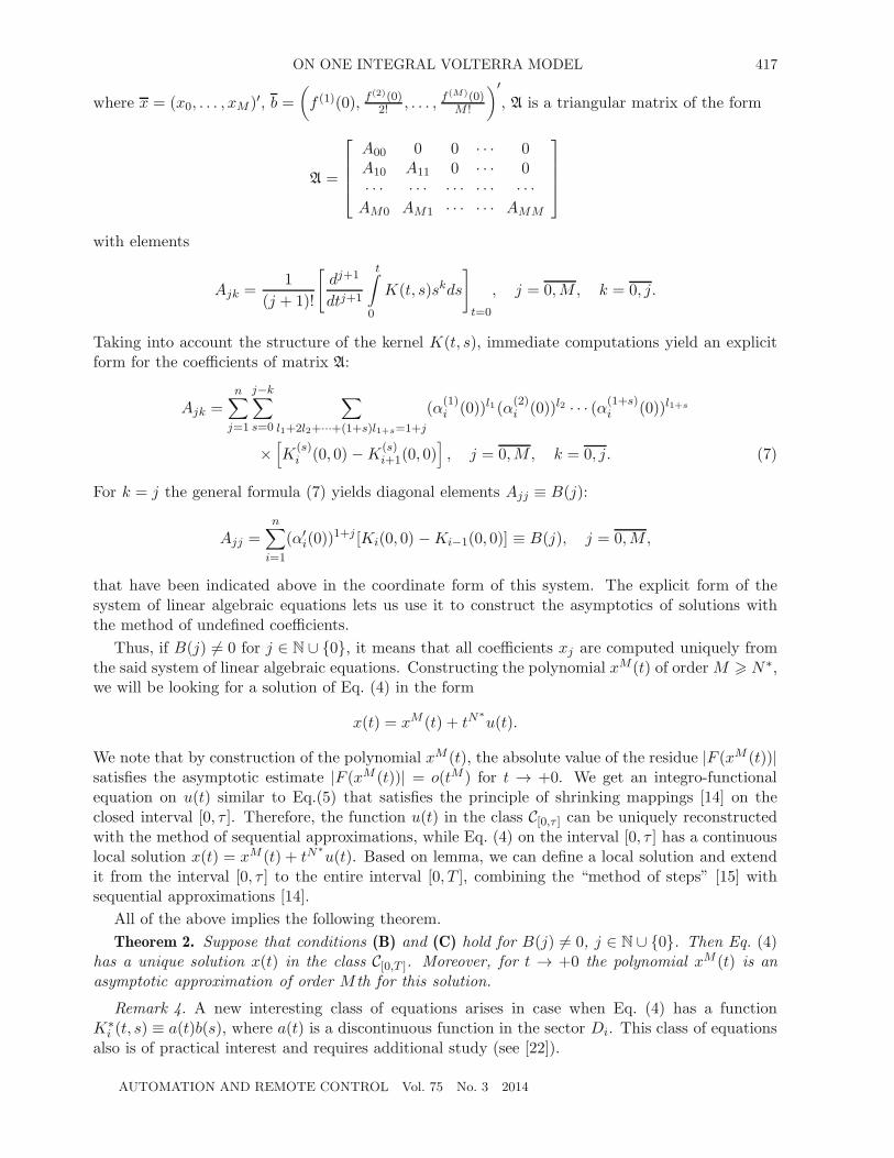
ON ONE INTEGRAL VOLTERRA MODEL 417
where x = (x0, . . . , xM )′, b =(f (1)(0), f
(2)(0)2! , . . . , f
(M)(0)M !
)′, A is a triangular matrix of the form
A =
⎡⎢⎢⎢⎣
A00 0 0 · · · 0A10 A11 0 · · · 0· · · · · · · · · · · · · · ·AM0 AM1 · · · · · · AMM
⎤⎥⎥⎥⎦
with elements
Ajk =1
(j + 1)!
[dj+1
dtj+1
t∫
0
K(t, s)skds
]
t=0
, j = 0,M, k = 0, j.
Taking into account the structure of the kernel K(t, s), immediate computations yield an explicitform for the coefficients of matrix A:
Ajk =n∑
j=1
j−k∑s=0
∑l1+2l2+···+(1+s)l1+s=1+j
(α(1)i (0))l1(α
(2)i (0))l2 · · · (α(1+s)
i (0))l1+s
×[K
(s)i (0, 0) −K
(s)i+1(0, 0)
], j = 0,M, k = 0, j. (7)
For k = j the general formula (7) yields diagonal elements Ajj ≡ B(j):
Ajj =n∑
i=1
(α′i(0))
1+j [Ki(0, 0) −Ki−1(0, 0)] ≡ B(j), j = 0,M,
that have been indicated above in the coordinate form of this system. The explicit form of thesystem of linear algebraic equations lets us use it to construct the asymptotics of solutions withthe method of undefined coefficients.
Thus, if B(j) �= 0 for j ∈ N ∪ {0}, it means that all coefficients xj are computed uniquely fromthe said system of linear algebraic equations. Constructing the polynomial xM(t) of order M � N∗,we will be looking for a solution of Eq. (4) in the form
x(t) = xM (t) + tN∗u(t).
We note that by construction of the polynomial xM (t), the absolute value of the residue |F (xM (t))|satisfies the asymptotic estimate |F (xM (t))| = o(tM ) for t → +0. We get an integro-functionalequation on u(t) similar to Eq.(5) that satisfies the principle of shrinking mappings [14] on theclosed interval [0, τ ]. Therefore, the function u(t) in the class C[0,τ ] can be uniquely reconstructedwith the method of sequential approximations, while Eq. (4) on the interval [0, τ ] has a continuouslocal solution x(t) = xM (t) + tN
∗u(t). Based on lemma, we can define a local solution and extend
it from the interval [0, τ ] to the entire interval [0, T ], combining the “method of steps” [15] withsequential approximations [14].
All of the above implies the following theorem.
Theorem 2. Suppose that conditions (B) and (C) hold for B(j) �= 0, j ∈ N ∪ {0}. Then Eq. (4)has a unique solution x(t) in the class C[0,T ]. Moreover, for t → +0 the polynomial xM (t) is anasymptotic approximation of order M th for this solution.
Remark 4. A new interesting class of equations arises in case when Eq. (4) has a functionK∗
i (t, s) ≡ a(t)b(s), where a(t) is a discontinuous function in the sector Di. This class of equationsalso is of practical interest and requires additional study (see [22]).
AUTOMATION AND REMOTE CONTROL Vol. 75 No. 3 2014
418 MARKOVA, SIDOROV
3. NUMERICAL METHODS
Consider a numerical solution for Eq. (4) in the case of two terms. Namely, consider an integralVolterra equation of the form
a(t)∫
0
K1(t, s)x(s)ds +
t∫
a(t)
K2(t, s)x(s)ds = f(t), t ∈ [0, T ], (8)
where 0 < a(t) < t ∀t ∈ (0, T ], a(0) = 0, functions K1(t, s), K2(t, s), f(t) are continuous and suffi-ciently smooth, f(0) = 0, K2(t, t) �= 0 ∀t ∈ [0, T ].
Theory and numerical methods for solving Eq. (8) for K1(t, s) ≡ 0 have been studied in detailin [7, 21]. Methods for numerical solution for linear Fredholm equations of the second kind withkernels that have discontinuities of the first kind on one or more continuous curves have beenconsidered in [23]. A characteristic feature of such equations requires one, in particular, to adaptnumerical procedures used for solving classical integral equations.
We use the method of right rectangles. We introduce a grid of nodes ti, i = 1, n, nh = T , and,approximating integrals in (8) with sums, write its grid counterpart in obvious notation:
hl−1∑j=1
K1(ti, tj)xh(tj) + (a(ti)− tl−1)K1(ti, a(ti))x
h(a(ti))
+(tl − a(ti))K2(ti, tl)xh(tl) + h
i∑j=l+1
K2(ti, tj)xh(tj) = f(ti), i = 1, n, (9)
where l =[a(ti)h
]+1. The appearance of terms that are not under the summation is caused by the
fact that the value of a(ti) in the general case does not fall exactly on a grid node.
Here already for n = 1 we have to solve one equation with two unknowns: xh(a(t1)) and xh(t1).A similar problem arises on every step except for special cases when a(ti) falls exactly on a grid node.To solve this problem, one can use different approaches, including a combination of the methodsof right and left rectangles, interpolation and extrapolation procedures, and also our knowledgeabout the solution of Eq. (8) at the initial point [18].
Numerical computations on test examples show that adapted methods converge linearly.
Example 1. Consider an example where the kernel includes the difference t− s, which reflects asystem’s attenuation, i.e., amortization or physical wear and tear of the capital (see, e.g., [24]):
t3∫
0
(1 + t− s)x(s)ds−t∫
t3
x(s)ds =t4
108− 25t3
81, t ∈ [0, 2],
the exact solution is x(t) = t2.
Table 1 shows the errors ε = max0�i�n |x(ti)− xh(ti)| for different steps.
Table 1. Errors of the numerical solution for test example 1
h ε
1/32 0.0666951/64 0.0341891/128 0.0173711/256 0.008652
AUTOMATION AND REMOTE CONTROL Vol. 75 No. 3 2014
ON ONE INTEGRAL VOLTERRA MODEL 419
0.35
0.30
0.25
0.20
0.15
0.10
0.05
0
–0.05
0.19
60.
393
0.58
90.
785
0.98
21.
178
1.37
41.
571
1.76
71.
964
2.35
62.
553
2.94
52.
749
3.14
23.
338
3.53
43.
731
3.92
74.
123
4.32
04.
516
4.71
24.
909
5.10
55.
301
5.49
85.
694
5.89
06.
087
6.28
30
t
Error Error for auxiliary grid
2.16
0
Fig. 1. Behavior of errors for example 2.
1.2
0
2π
a
( t )
π
1.00.80.60.40.2
Fig. 2. Graph of the lower limit a(t) = sint
2in Example 2.
Example 2.
2
sin t2∫
0
x(s)ds+
t∫
sin t2
x(s)ds =1
3sin3
t
2+
t3
3, t ∈ [0, 2π],
the exact solution is x(t) = t2.
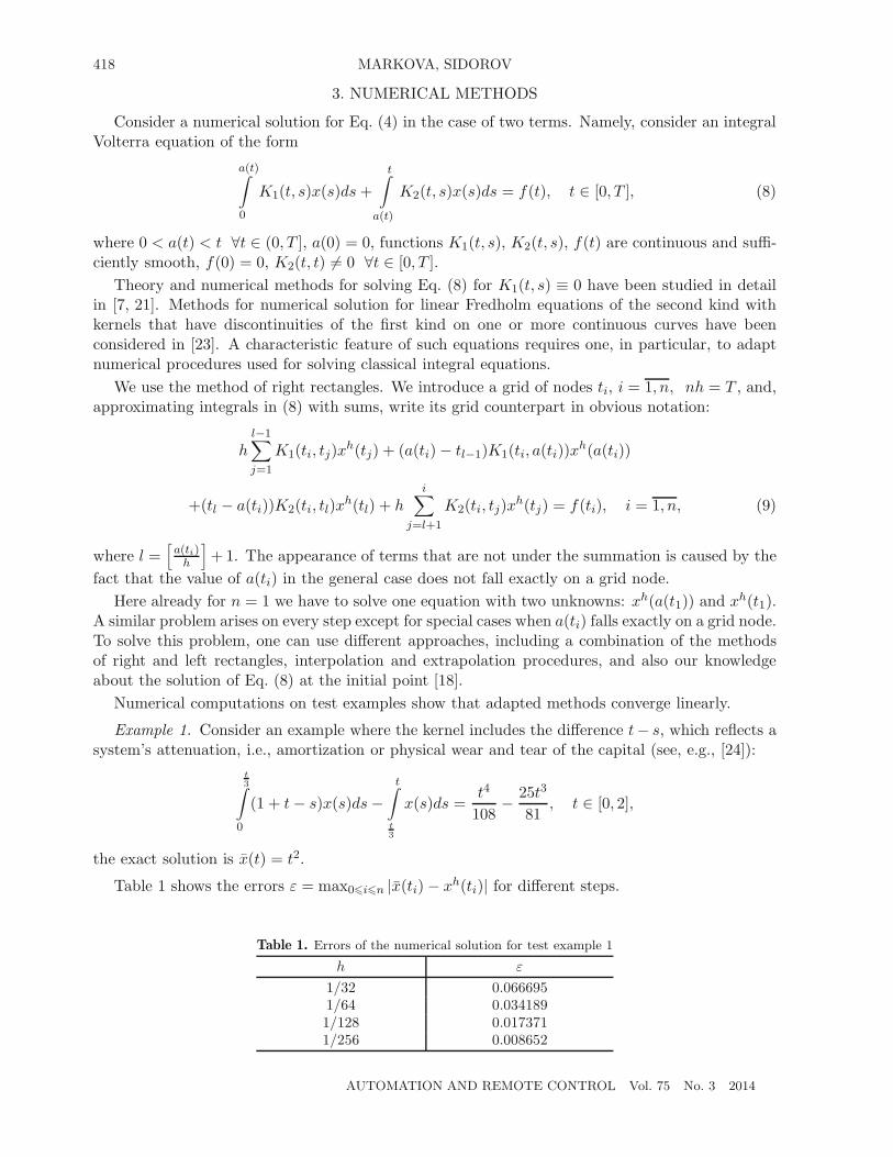
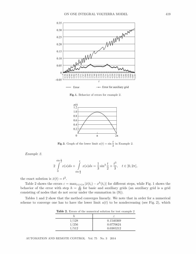
Table 2 shows the errors ε = max1�i�n |x(ti)− xh(ti)| for different steps, while Fig. 1 shows thebehavior of the error with step h = π
64 for basic and auxiliary grids (an auxiliary grid is a gridconsisting of nodes that do not occur under the summation in (9)).
Tables 1 and 2 show that the method converges linearly. We note that in order for a numericalscheme to converge one has to have the lower limit a(t) to be nondecreasing (see Fig. 2), which
Table 2. Errors of the numerical solution for test example 2
h ε
1/128 0.15403691/256 0.07706241/512 0.0385212
AUTOMATION AND REMOTE CONTROL Vol. 75 No. 3 2014
420 MARKOVA, SIDOROV
is compatible with Remark 2 and lets us construct models without a rigid requirement that thecurves αi(t), which describe the time moment when equipment (a unit of capital) must be put outof use, are nondecreasing [24].
4. CONCLUSION
In this work, we have developed an approach for constructing parametric families of continuoussolutions of integral Volterra equations of the first kind that arise in modeling developing systems.We have studied, both analytically and numerically, the regular case when the characteristic equa-tion does not have natural roots, and the solution of the integral equation is unique. We giveexistence theorems for the solutions and study their asymptotic behavior.
Theoretical results are illustrated with numerical computations on test examples. We show thatan adapted method of right rectangles has linear convergence.
ACKNOWLEDGMENTS
This work was supported by the Ministry of Education and Science of the Russian Federation,the Federal Goal-oriented Program “Scientific and Educational Personnel of Innovative Russia”(state contract no. 14.V37.21.0365), Deutscher Akademischer Austauschdienst (DAAD), projectno. A1200665, and the Russian Foundation for Basic Research, project no. 12-01-00722-a.
The authors are grateful to the anonymous referees for their remarks that have improved thepaper. The second author is grateful to Prof. Alfredo Lorenzi (Universita degli Studi di Milano)for a useful discussion of the results of this work.
REFERENCES
1. Glushkov, V.M., On One Class of Dynamical Macroeconomical Models, Upravl. Sist. Mashiny, 1977,no. 2. pp. 3–6.
2. Glushkov, V.M., Ivanov, V.V., and Yanenko, V.M., Modelirovanie razvivayushchikhsya sistem (ModelingDeveloping Systems), Moscow: Nauka, 1983.
3. Yatsenko, Yu.P., Integral’nye modeli sistem s upravlyaemoi pamyat’yu (Integral Models for Systems withControllable Memory), Kiev: Naukova Dumka, 1991.
4. Hritonenko, N. and Yatsenko, Yu., Modeling and Optimization of the Lifetime of Technologies, Dordrecht:Kluwer, 1996.
5. Hritonenko, N. and Yatsenko, Yu., Integral Equation of Optimal Replacement: Analysis and Algorithms,Appl. Math. Model, 2009, vol. 33, no. 6, pp. 2737–2747.
6. Boikov, I.V. and Tynda, A.M., Approximate Solution of Nonlinear Integral Equations of the Theory ofDeveloping Systems, Differ. Equat., 2003, vol. 9, pp. 1277–1288.
7. Denisov, A.M. and Lorenzi, A., On a Special Volterra Integral Equation of the First Kind, Boll. Un.Mat. Ital. B, 1995, vol. 7, no. 9, pp. 443–457.
8. Apartsyn, A.S., Markova, E.V., and Trufanov, V.V., Integral Models of Development for ElectricalEnergy Systems, Preprint of Melentiev Energy Systems Inst., Irkutsk, 2002, no. 1.
9. Karaulova, I.V. and Markova, E.V., On One Optimal Control Problem in the Glushkov Type IntegralModels, Proc. Forth Int. Conf. “Inverse Probl.: Identificat., Design and Control,” July 2–6, 2003,Moscow, CD-proceedings.
10. Karaulova, I.V., Markova, E.V., Trufanov, V.V., et al., On Modeling the Development of ElectricalEnergy Systems with Integral Models, in Nauchn. Tr. “Metody issledovaniya i modelirovaniya tekhni-cheskikh, sotsial’nykh i prirodnykh sistem” (Proc. “Methods of Studying and Modeling Technical, Social,and Natural Systems”), Novosibirsk: Nauka, 2003, pp. 85–100.
AUTOMATION AND REMOTE CONTROL Vol. 75 No. 3 2014
ON ONE INTEGRAL VOLTERRA MODEL 421
11. Ivanov, D.V., Karaulova, I.V., Markova, E.V., Trufanov, V.V., and Khamisov, O.V., Control of PowerGrid Development: Numerical Solutions, Autom. Remote Control, 2004, vol. 65, no. 3. pp. 472–482.
12. Apartsyn, A.S., Karaulova, I.V., Markova, E.V., et al., Using Integral Volterra Equations to ModelStrategies of Technical Reequipment of Electrical Power Industry, Elektrichestvo, 2005, no. 10. pp. 69–75.
13. Karaulova, I.V. and Markova, E.V., Optimal Control Problem of Development of an Electric PowerSystem, Autom. Remote Control, 2008, vol. 69, no. 4, pp. 637–644.
14. Trenogin, V.A., Funktsional’nyi analiz (Functional Analysis), Moscow: Fizmatlit, 2007.
15. El’sgol’ts, L.A., Kachestvennye metody v matematicheskom analize (Qualitative Methods in Calculus),Moscow: GITTL, 1955.
16. Sidorov, D.N., On Feasibility of Volterra Equations of the First Kind with Piecewise Continuous Kernelsin the Class of Generalized Functions, Izv. Irkutsk. Gos. Univ., Ser. Mat., 2012, vol. 5, no. 1, pp. 80–95.
17. Sidorov, D.N., On Feasibility of Systems of Integral Volterra Equations of the First Kind with PiecewiseContinuous Kernels, Izv. Vyssh. Uchebn. Zaved., Mat., 2013, no. 1, pp. 62–72.
18. Markova, E.V. and Sidorov, D.N., Integral Volterra Equations of the First Kind with Piecewise Contin-uous Kernels in the Theory of Modeling Developing Systems, Izv. Irkutsk. Gos. Univ., Ser. Mat., 2012,no. 2, pp. 31–45.
19. Sidorov, D., Volterra Equations of the First Kind with Discontinuous Kernels in the Theory of EvolvingSystems Control, Studia Informat. Universal., 2011, vol. 9, no. 3, pp. 135–146.
20. Sidorov, D.N., Slabo singulyarnye uravneniya Vol’terra pervogo roda: teoriya i prilozheniya v modeliro-vanii razvivayushchikhsya dinamicheskikh sistem (Weakly Singular Volterra Equations of the First Kind:Theory and Applications in Modeling Developing Dynamical Systems), Saarbrucken: Palmar. Academ.Publish., 2012.
21. Apartsyn, A.S., Nonclassical Linear Volterra Equations of the First Kind, Utrecht: VSP, 2003.
22. Apartsyn, A.S., On One Approach to Modeling Developing Systems, Nauchn. Tr. 6 Mezhd. nauchn. sem-inara “Obobshchennye postanovki i resheniya zadach upravleniya” (Proc. 6th Int. Sci. Seminar “Gener-alized Settings and Solutions of Control Problems”), IFAC GSSCP-2012, Gelendzhik, Russia, September25–27, 2012 (CD).
23. Micke, A., The Treatment of Integral Equations with Discontinuous Kernels Using Product TypeQuadrature Formulas, Computing, 1989, no. 42, pp. 207–223.
24. Hritonenko, N. and Yatsenko, Yu., Turnpike and Optimal Trajectories in Integral Dynamic Models withEndogenous Delay, J. Optim. Theory Appl., 2005, vol. 127, no. 1, pp. 109–127.
This paper was recommended for publication by V.I. Gurman, a member of the Editorial Board
AUTOMATION AND REMOTE CONTROL Vol. 75 No. 3 2014