on oscillating ﬂows in randomly heterogeneous porous...

Phil. Trans. R. Soc. A (2010) 368, 197–216doi:10.1098/rsta.2009.0186

On oscillating flows in randomly heterogeneousporous media

BY M. G. TREFRY1,2,*, D. McLAUGHLIN3, G. METCALFE4, D. LESTER4,A. ORD2,5, K. REGENAUER-LIEB2,5 AND B. E. HOBBS2,5

1CSIRO Land and Water, Private Bag 5, Wembley WA 6913, Australia2School of Earth and Environment, University of Western Australia,

35 Stirling Highway, Crawley, Perth WA 6009, Australia3Department of Civil and Environmental Engineering, Massachusetts Institute

of Technology, Cambridge, MA 02139, USA4CSIRO Materials Science and Engineering, PO Box 56,

Highett VIC 3190, Australia5CSIRO Exploration and Mining, PO Box 1130, Bentley WA 6102, Australia

The emergence of structure in reactive geofluid systems is of current interest. In geofluidsystems, the fluids are supported by a porous medium whose physical and chemicalproperties may vary in space and time, sometimes sharply, and which may also evolve inreaction with the local fluids. Geofluids may also experience pressure and temperatureconditions within the porous medium that drive their momentum relations beyond thenormal Darcy regime. Furthermore, natural geofluid systems may experience forcings thatare periodic in nature, or at least episodic. The combination of transient forcing, near-critical fluid dynamics and heterogeneous porous media yields a rich array of emergentgeofluid phenomena that are only now beginning to be understood. One of the barriers toforward analysis in these geofluid systems is the problem of data scarcity. It is most oftenthe case that fluid properties are reasonably well known, but that data on porous mediumproperties are measured with much less precision and spatial density. It is common toseek to perform an estimation of the porous medium properties by an inverse approach,that is, by expressing porous medium properties in terms of observed fluid characteristics.In this paper, we move toward such an inversion for the case of a generalized geofluidmomentum equation in the context of time-periodic boundary conditions. We showthat the generalized momentum equation results in frequency-domain responses thatare governed by a second-order equation which is amenable to numerical solution. Astochastic perturbation approach demonstrates that frequency-domain responses of thefluids migrating in heterogeneous domains have spatial spectral densities that can beexpressed in terms of the spectral densities of porous media properties.

Keywords: geofluids; heterogeneity; porous medium; stochastic; spectral density

*Author for correspondence ([email protected]).

One contribution of 17 to a Theme Issue ‘Patterns in our planet: applications of multi-scalenon-equilibrium thermodynamics to Earth-system science’.

This journal is © 2010 The Royal Society197

on July 28, 2018http://rsta.royalsocietypublishing.org/Downloaded from

mailto:[email protected]

http://rsta.royalsocietypublishing.org/

198 M. G. Trefry et al.

1. Introduction

The migration of geofluids in the porous subsurface is of fundamental scientificimportance and of considerable economic and environmental relevance to society.Many basic principles underlying flow and transport in porous media havebeen established, allowing widespread mineral and water resource exploitationand engineering in the regolith. However, as the world population grows andresource exploitation continues, prospective resources are becoming scarce.Increasingly, geofluid theories are being re-examined to improve the efficiency ofcharacterization and prediction of the scale and quality of subsurface resources.One of the key recent advances is the explicit coupling of fluid dynamics withadvanced geodynamic equations of state and with sophisticated biogeochemicalreaction systems. This has allowed researchers to grasp the complexity offluid–rock interactions and to note emergence of structure as a critical dynamic.Examples of emergence may include the creation of orebodies through promotedgeochemical reactions, and oscillating opening and sealing of fault aperturesthrough cyclic pumping of reactive fluids.

The complexity that gives rise to structural emergence can be embodiedwithin the governing mathematical operators describing the physical processes,or through geometric properties of the system of interest. In seeking to establishorganizational principles, it is important to understand relationships betweenpatterns in the system. In this paper, we take a geometric view of a porousmedium and seek to understand how spatial patterns of the porous mediumproperties will influence the spatial and temporal characteristics of a fluid filteringthrough under the influence of periodic boundary conditions. Our thesis is thatemergence in natural systems is a function of both the nature of the local geofluidprocesses and of the structure of the supporting medium, and that in order tounderstand the generation of emergence, it will often be important to understandboth the processes and the structure.

As an initial step to characterizing geometric influences on fluid migration,we consider the filtration of a fluid through a heterogeneous porous medium.To provide as much generality to the fluid process description as possible, wefirst identify a generalized constitutive relation for the fluid filtration and fromit derive a governing equation for the propagation of boundary modes throughthe non-deforming porous medium. Typically, spatial data on the properties ofthe porous medium are scarce, which limits the ability to build comprehensivegeofluid models. Spectral techniques are common means of correlating patternsat like scales, and are thus useful in inferring structure between correlated signalswhere data coverage is uneven. Here, a stochastic spatial structure is employedfor the properties of the porous medium and a perturbation approach is used toderive a relationship between the spatial spectra of the porous medium propertiesand the fluid dependent variable. As shown, there is good prospect that thisrelationship is invertible, allowing the geometric structure of the porous mediumto be estimated from observations of scalar fluid properties.

2. Generalized constitutive equation

We consider a non-turbulent fluid undergoing oscillating motion within a porousmedium, and seek to generalize the fluid constitutive relation in order to capture

Phil. Trans. R. Soc. A (2010)



Oscillating flows in random porous media 199

a range of phenomena that may potentially apply in geofluid systems. In thesimplest limit, the Darcy equation (Darcy 1856; Freeze 1994) relates the fluidflux vector, J , to the local pressure gradient, ∇P,

J = −κ

η∇P, (2.1)

that is, the flow is laminar and the fluid flux is proportional to the fluid pressuregradient. Note that, for large pressure gradients, inertial forces may outweighviscous drag on pore boundaries and the flow may become turbulent (e.g. Furbish1996). This is most often the case for large pore diameters (secondary porosityfeatures and large aperture faults) where the Darcy equation no longer applies.Equation (2.1) is mathematically similar to Fick’s law for diffusing solutes andFourier’s law for heat conduction, so, in the spirit of generalization, we will replacethe pressure P by the scalar dependent variable u, and refer to κ simply as thepermeability and η as viscosity. The permeability is a property of the porousmedium, while the viscosity is a fluid property. Equation (2.1) can be combinedwith the linear continuity equation

λ∂u∂t

= −∇ · J , (2.2)

where λ is a volumetric capacity coefficient, to yield the usual dynamical equation

λ∂u∂t

= ∇ ·(

κ

η∇u

). (2.3)

Extensions to the linear constitutive relation (2.1) are common. Brinkman(1947) proposed the addition of a viscous drag term to model frictional forcesacting on a steady fluid at grain boundaries

J = −κ

η∇u + β2κ∇2J . (2.4)

Here, the non-negative quantity β is defined by β2 ≡ η′/η, the ratio of the effectiveviscosity averaged over the local flow within the pore space (η′) to the bulk fluidviscosity. In the absence of further information regarding grain-boundary frictionaveraging, β2 is often assumed to be unity, although Brinkman (1947) providesother possible estimates. As discussed by Capuani et al. (2003), this term is onlyjustified for media with porosity close to unity, but has been shown to be usefulfor describing steady viscous flows in inhomogeneous systems, including biologicaltissues (Khaled & Vafai 2003).

Temporal modifications to the fluid constitutive relation are also ofinterest, since they allow a greater range of time-dependent phenomena tobe modelled than are supported by equation (2.1). For example, the diffusivedynamical equation (2.3) admits unphysical infinite propagation of disturbances(Compte & Metzler 1997), a situation for which Cattaneo (1958) proposed theconstitutive relation

J + τ∂J∂t

= −κ∇u. (2.5)

The non-negative quantity τ is a relaxation parameter that governs thetemporal equilibration interval for disturbances to the flux J . A similar relationwas obtained by Maxwell (1867) in connection with the kinetic theory of





gases, and was elaborated by Grad (1958). This relation, combined with thecontinuity equation (2.2), yields the well-known dissipating wave equation ortelegrapher’s equation

λτ∂2u∂t2

+ λ∂u∂t

= ∇ · (κ∇u). (2.6)

Through the hyperbolic form of equation (2.6), the effect of the temporalderivative of equation (2.5) is to ensure that wave-like disturbances in the flowfield propagate with velocity

√κ/λτ (King et al. 1998). The dissipating wave

equation is widely used to describe finite correlation-time phenomena in diverseareas of physics, including granular system stress dynamics (Scott et al. 1998),the so-called second sound of thermo-acoustics (Chester 1963), heat conductionand thermo-elasticity (Marín et al. 2002; Khisaeva & Ostoja-Starzewski 2006)and in chemical reaction–diffusion (Manne et al. 2000).

Other temporal models are possible. Khuzhayorov et al. (2000) noted thephenomenological filtration model

J = −κ

η

(1 + ε

∂

∂t

)∇u, (2.7)

which incorporates a non-negative retardation parameter ε to modulate temporalchanges in the state variable u. Such a constitutive relation was used by Tan(2006) to describe overshoot phenomena in viscoelastic fluids, and Wang & Tan(2008) used the same relation to perform a stability analysis for double-diffusivethermal convection of a Maxwell fluid. In analogy with the constitutive relationfor an Oldroyd-B fluid, Alishaev & Mirzadjanadze (1975) introduced the dualtemporal gradient relation(

1 + τ∂

∂t

)J = −κ

η

(1 + ε

∂

∂t

)∇u, (2.8)

which has since been widely applied in rheology, geophysics and in industrialapplications (Tan & Masuoka 2005). Khuzhayorov et al. (2000) apply an upscalingtechnique to derive a macroscopic filtration law valid for low Reynolds andDeborah numbers that incorporates Oldroyd-B phenomena as a special case.They question the viability of equation (2.8) to model the filtration of Oldroyd-Bfluids, since the predictions of their macroscopic law depart strongly from thoseof the phenomenological model (2.8). Nevertheless, equation (2.8) continues tobe used to model viscoelastic convection phenomena in porous media, with theconvective onset properties now well understood (Kim et al. 2003). More recentdevelopments include the use of fractional derivative forms of equation (2.8)to model transient stress relationships in generalized Burgers’ fluids (Khan &Hayat 2008; Xue et al. 2008), and the potential for convective instability indoubly diffusive systems exposed to constant fluid throughflow (Shivakumara &Sureshkumar 2008).

In pursuing a simplified filtration model of viscoelastic flow in porous media,we propose the following generalized relationship for a single fluid-state variableu subject to Brinkman viscous drag (enhanced dissipation) and dual temporalrelaxation–retardation phenomena:(

1 + τ∂

∂t− β2κ∇2

)J = −κ

(1 + ε

∂

∂t

)∇u. (2.9)





Here, we have absorbed viscosity η into the definition of κ. The hope is thatthis constitutive relation is flexible enough to describe a range of non-Darcianflow phenomena in heterogeneous porous media, but remains simple enough toyield analytical estimates of stochastic relationships in the spatial and temporalfrequency domains. As we shall see, the linear nature of equation (2.9) is sufficientto ensure that such spectral relationships can be obtained in suitable limits. Chiefamong the limiting assumptions is the neglect of any explicit constitutive relationbetween the fluid stress and strain tensors, i.e. the filtration approximation.In justifying this assumption, we appeal to the limit of laminar Darcy flow,that is, where the effects of stress–strain relationships are small and can bemodelled through a simple momentum law such as equation (2.9). In makingthis assumption, we expressly rule out turbulent effects associated with high-velocity flow through large voids. For broader application, it is understood thatthe general scalar state variable u may variously be associated with fluid pressure,concentration or temperature, according to practical context.

3. Modal dynamics in heterogeneous systems

Geological porous media display heterogeneity. In our model, we will seekto represent heterogeneity by allowing our material property parameters tovary in space. In particular, we deem the permeability κ, relaxation τ andretardation ε to take the form of random functions of location. We also assumethat the Brinkman term is such that the fully heterogeneous Brinkman formmay be approximated as ∇ · (β2κ(x)∇J ) ≈ β2κ(x)∇ · ∇J , i.e. Brinkman dragis modelled as a homogeneous correction term. Furthermore, we assume thecapacity coefficient λ to be uniform and homogeneous. Spatial heterogeneityof the Brinkman and capacity coefficients may be included at the expense ofgreater algebraic complexity. Derivation of the dynamical equation follows theusual approach of substitution of equation (2.9) in the continuity equation (2.2),yielding

∇ · (τJ t) + λut = ∇ · [κ(−β2∇2J + ε∇ut + ∇u)]. (3.1)

Since we are most interested in oscillating flows, we transform to frequency spaceusing the Fourier transformation rule

F t,ω[h(t)] ≡ h(ω) = 1√2π

∫∞

−∞heiωt dt, (3.2)

where h(t) is required to be integrable over time. It then follows that F t,ω[ht] ≡iωh and F t,ω[htt] ≡ −ω2h. Transforming equations (2.2), (2.9) and (3.1), andtaking repeated spatial derivatives of the continuity equation to eliminate Jand its derivatives from equation (3.1) eventually yields the following governingequation for u responding to the frequency mode ω:

∇ · (κ∇u) +(

ωκ

i − ωτ∇τ + iωκ

1 + iεω + iβ2λω∇ε

)· ∇u − λω(i − ωτ)

1 + iεω + iβ2λωu = 0.

(3.3)This hyperbolic equation describes how the Fourier coefficient of u for frequency ωvaries spatially within the porous medium in response to spatial variations in κ, τand ε. In the diffusive limit β2 = τ = ε = 0, the governing equation reduces to the





usual Helmholtz form for damped oscillations ∇ · (κ∇u) − iλωu = 0, which is wellstudied for oscillating modes in groundwater hydrology and heat conduction. Ifthe relaxation and retardation fields have zero gradients, the governing equationcan be written ∇ · (κ∇u) − k2u = 0, where k can be identified as the complexwavenumber of the oscillation, satisfying k = √

λω(i − ωτ)/(1 + iεω + iβ2λω).The real and imaginary parts of k display most curvature for small ω. Since thereal parts of the solutions of (3.3) are oscillatory, it is usually helpful to classifytheir behaviour in terms of oscillation amplitude, |u|, and phase θ = arg(u).Townley (1995) provides a useful mapping of the phase into units of oscillationperiods, denoted Φ,

Φ(θ) =

⎧⎪⎨⎪⎩

1 − θ

2π, for 0 < θ ≤ 2π ,

− θ

2π, for − π ≤ θ ≤ 0.

(3.4)

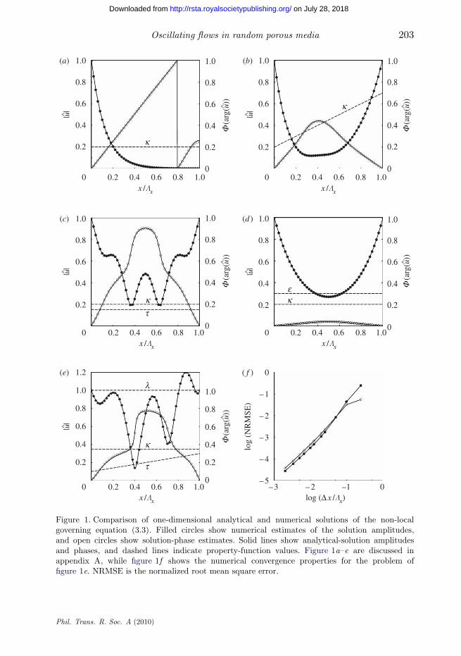
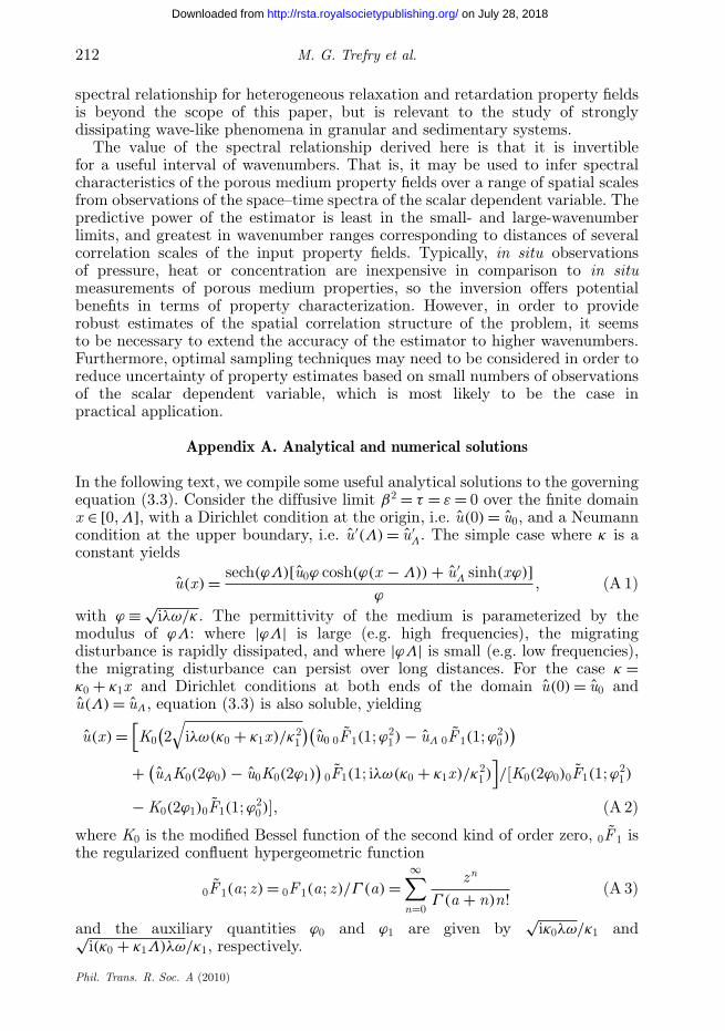
The governing equation (3.3) may be integrated analytically for special classesof the spatial variations of κ, τ and ε, and is amenable to numerical solutionby standard finite-difference techniques. Appendix A discusses analytical andnumerical solution of equation (3.3) in more detail. Figure 1 shows that a simplecentral-difference approach provides useful approximations to a wide range ofdissipating wave phenomena generated by equation (3.3), and is sufficient to yieldnear-second-order convergence for underdamped waves with a spatially variablerelaxation function τ .

4. Spatial correlation in the weakly hyperbolic model

Having derived the equation governing the propagation of frequency modesthrough our generalized fluid, we are now in a position to consider how the spatialstatistics of the porous medium may influence the properties of the propagatingmodes. One approach to this would be to simply generate a set of realizationsof κ, τ and ε fields (according to specified internal correlation structures), runthem through a numerical solver to generate the corresponding u solutions and tocross correlate these against the input fields. This is a computationally expensiveapproach. Instead, we seek to derive, from first principles, a statistical correlationbetween the input and output fields that is independent of the internal correlativestructures of the input fields. In order to do so, we will have to make a range ofassumptions regarding the strength of the relaxation/retardation and dissipativeterms in equation (3.3).

We commence by regarding κ, τ , ε and u as spatially random fields that arestationary, that is, their means are well defined over the domain of interest withno drift terms. Consequently, we can decompose the property and solution fieldsinto means and fluctuations (δ) as follows:

log κ = F = 〈F〉 + δF ,

log τ = V = 〈V 〉 + δV ,

log ε = W = 〈W 〉 + δW ,

and u = 〈u〉 + δu.

⎫⎪⎪⎪⎬⎪⎪⎪⎭

(4.1)





1.0(a) (b)

(c) (d )

(e) ( f )

0.8

0.6

0.4

0.2

0

0.2 0.4x /Λx log (Δ x /Λx)

log

(NR

MSE

)

0.6 0.8 1.0

0.2 0.4x /Λx

0.6 0.8 1.0

0.2 0.4x /Λx

0.6 0.8 1.0

0.2 0.4x /Λx

0.6 0.8 1.0

0.2 0.4x /Λx

0.6 0.8 1.0

– 3 – 2 –1 0

|u∧ |1.0

0.8

0.6

0.4

0.2

0

|u∧ |

1.0

0.8

0.6

0.4

0.2

0

|u∧ |

1.0

0.8

0.6

0.4

0.2

0

|u∧ |

1.0

1.2

0.8

0.6

0.4

0.2

0– 5

– 4

– 3

– 2

– 1

0

|u∧ |1.0

0.8

0.6

0.4

0.2

0

1.0

0.8

0.6

0.4

0.2

0

1.0

0.8

0.6

0.4

0.2

0

F (a

rg(u∧ ))

F (a

rg(u∧ ))

F (a

rg(u∧ ))

F (a

rg(u∧ ))

F (a

rg(u∧ ))

1.0

0.8

0.6

0.4

0.2

0

1.0

0.8

0.6

0.4

0.2

0

k

k

kt

t

l

k

k

e

Figure 1. Comparison of one-dimensional analytical and numerical solutions of the non-localgoverning equation (3.3). Filled circles show numerical estimates of the solution amplitudes,and open circles show solution-phase estimates. Solid lines show analytical-solution amplitudesand phases, and dashed lines indicate property-function values. Figure 1a–e are discussed inappendix A, while figure 1f shows the numerical convergence properties for the problem offigure 1e. NRMSE is the normalized root mean square error.





In equation (4.1), we have made a log transformation for all non-negativeparameters. Denoting the geometric mean by the subscript ‘G’, 〈F〉 = log κG,〈V 〉 = log τG and 〈W 〉 = log εG, the decompositions can be expressed as

κ = κGeδF , τ = τGeδV and ε = εGeδW . (4.2)

Since the property fields are now random variables, equation (3.3) requiressome rationalization in order to proceed with the analysis. In particular, we notethe denominators (i − ωτ) and (1 + iεω + iβ2λω) and introduce the concept ofweakly hyperbolic dynamics, that is where ωτ � 1 (weak temporal relaxation) andwhere both ωε � 1 and β2λω � 1 (weak temporal retardation and weak Brinkmandissipation, respectively). In these domains, the denominators can be expandedto first order, yielding the weakly hyperbolic form of equation (3.3)

∇ · (κ∇u) + ωκ((−i − ωτ)∇τ + (i + εω + β2λω)∇ε) · ∇u

− λω(i − ωτ)(1 − iεω − β2λω)u = 0. (4.3)

Substituting equation (4.2) and neglecting gradients of the field means(a stationarity assumption) yields

− λω(1 − iω(β2λ + εGeδW ))(i − ωτGeδV )(〈u〉 + δu)

+ κGeδF∇δF(∇〈u〉 + ∇δu) + [ωκGτGeδF+δV (−i − ωτGeδV )∇δV

+ ωκGεGeδF+δW (i + ωβ2λ + ωεGeδW )∇δW ](∇〈u〉 + ∇δu)

+ κGeδF (∇2〈u〉 + ∇2δu) = 0. (4.4)

We now assume that the spatial fluctuations are small (a low-varianceassumption), so that the exponential terms can be linearized,

eδF ≈ 1 + δF , eδV ≈ 1 + δV and eδW ≈ 1 + δW . (4.5)

Substituting equation (4.5) into equation (4.4), discarding terms containingsecond-order and higher products of fluctuations, and noting the mean solution〈u〉 satisfies

κG∇2〈u〉 − λω(i − ωτG)(1 − iεGω − β2λω)〈u〉 = 0, (4.6)

leads eventually to

− iλω(i + β2λω + ωεG)(−i + ωτG)δu − iλω2τG(i + β2λω + ωεG)δV 〈u〉+ λω2εG(−1 − iωτG)δW 〈u〉 + κG∇δF∇〈u〉 − ωκGτG(i + ωτG)∇δV∇〈u〉+ ωκGεG(i + β2λω + ωεG)∇δW∇〈u〉 + κG∇2δu + κGδF∇2〈u〉 ≈ 0. (4.7)

We can identify further terms that are small. By the weakly hyperbolic andlow-variance assumptions, the term −iλω2τG(i + β2λω + ωεG)δV 〈u〉 � ω〈u〉 andcan be neglected. Also, λω2εG(−1 − iωτG)δW 〈u〉 can be shown to be similarly





small and can be neglected. With these reductions and defining the convenientparameter α = i + β2λω + ωεG, we obtain

− iαλω(−i + ωτG)δu + κG∇2δu + κGδF∇2〈u〉+ κG∇〈u〉(∇δF − ωτG(i + ωτG)∇δV + αωεG∇δW ) ≈ 0. (4.8)

The spatial spectral characteristics of the property fluctuations must be resolved.We pursue the following Fourier transformation into reciprocal space measuredby the wavevector k:

Fx ,k [h(x)] ≡ h(k) = 1√2π

∫∞

−∞heik·x dx . (4.9)

Equation (4.8) contains several terms that are products of space-dependentfunctions. In order to pursue spectral integration, we need to consider these formsexplicitly. First, we consider the wavenumber transform of the term κGδF∇2〈u〉.Integration by parts yields

Fx ,k [κGδF∇2〈u〉] = κG(δF∇〈u〉|∞−∞ − Fx ,k [∇δF∇〈u〉] − ikFx ,k [δF∇〈u〉]).(4.10)

We can reduce equation (4.10) by noting that ∇〈u〉 → 0 as |x| → ∞ for alldissipative processes, so the first term in parentheses vanishes. Secondly, weare most interested in observed spectral properties near a forcing boundary,i.e. where the signal to noise ratio will be high enough to discriminate propertyfluctuations. With this proximity assumption, we may approximate the gradientof the mean response by a constant, i.e. ∇〈u(x)〉 ≈ ∇u0. Hence, it is easy toshow that

Fx ,k [κGδF∇2〈u〉] ≈ −2ikκG∇u0Fx ,k [δF ]= −2ikκG∇u0dZδF , (4.11)

where dZδF is the Fourier–Stieltjes increment (defined with support k) ofthe random process δF (defined with support x). Parra et al. (1999)discuss application of Fourier–Stieltjes forms to acoustic-wave propagation inheterogeneous systems. Applying the proximity limit equation (4.11) to theremainder of equation (4.8) and rearranging yields the following spectralrelationship, expressed in Fourier–Stieltjes notation:

dZδu ≈ κG∇u0 k(−idZδF + iαωεGdZδW + ωτG(1 − iωτG)dZδV )

αλω + κGk2 + iαλω2τG. (4.12)

The Wiener–Khinchine theorem expresses the spectral density Shh associatedwith the Fourier–Stieltjes increment dZh of a function h,

Shh = 〈dZhdZ∗h〉. (4.13)





Thus, equation (4.12) readily admits the following expression for the spectraldensity of δu:

Sδuδu dk ≈ κ2G|∇u0|2k2

k4κ2G + λω2(λ + 2k2κG(ς − τG)) + λ2ω4(ω2τ 2

Gς2 + ς2 + τ 2G)

×

⎛⎜⎜⎜⎝

SδFδF + ω2[ε2GSδW δW − εGςSδW δF

+ τG(−εGSδW δV + τGSδV δV + τG(SδV δF + SδFδV ))− εG(ςSδFδW + τGSδV δW ) + iωεGτG(ς − τG)(SδW δV − SδV δW )]

+ ω4[τ 4GSδV δV + ε2

Gς2SδW δW − εGτ 2Gς(SδW δV + SδV δW )]

+ iω[εG(SδFδW − SδW δF ) + τG(SδV δF − SδFδV )]

⎞⎟⎟⎟⎠ dk,

(4.14)

where ς ≡ β2λ + εG.Equation (4.14) provides a first-order expansion of the spatial spectral density

of the modal fluctuation u in terms of the spatial cross-spectral densities of theproperty fields κ, τ and ε. The full equation is complicated, but admits somespecial cases. In the case of uncorrelated property fields (which may not apply inmany practical situations) the cross-spectral densities have zero means, yielding

Sδuδu dk ≈ κ2G|∇u0|2k2(SδFδF + ω2τ 2

G(1 + ω2τ 2G)SδV δV + ω2ε2

G(1 + ω2ς2)SδW δW )

k4κ2G + λω2(λ + 2k2κG(ς − τG)) + λ2ω4(ω2τ 2

Gς2 + τ 2G + ς2)

dk.

(4.15)Simple diffusion/conduction phenomena, e.g. Darcy flows or heat conduction, canbe recovered in the limit εG = τG = β2 = 0,

Sδuδu dk ≈ κ2G|∇u0|2k2SδFδF

k4κ2G + λ2ω2

dk, (4.16)

while Darcy–Brinkman flows can be recovered in the limit εG = τG = 0,

Sδuδudk ≈ κ2G|∇u0|2k2SδFδF

k4κ2G + λω2(λ + 2k2β2λκG + λ4ω4β4)

dk. (4.17)

It is not until retardation and/or relaxation phenomena are enabled that cross-spectral terms appear in the modal spectral density (4.14). It is also notable thatequation (4.14) tends to zero with k, that is, the perturbative approximationis unable to resolve long-wavelength structures. This constraint arises from theearlier spatial stationarity assumption.

5. Robustness of the proximity assumption

The usefulness of the spectral density relationships derived in the previoussection hinges on the robustness of the proximity assumption discussed priorto equation (4.11), i.e. the validity of the approximation ∇〈u(x)〉 ≈ ∇u0. Thepotential usefulness of this assumption is promoted by the weakly hyperbolic





approximation that renders the system more strongly dissipative than wave-like,thus reducing the occurrence of standing wave patterns that may generatestrongly varying gradients in the mean response. In the following, we demonstratethat a mean value estimate of ∇u0 is sufficient to provide useful agreementbetween the input permeability spectrum and the observed modal fluctuation forsystems corresponding to equation (4.16). The demonstration is performed bycalculating the modal fluctuation δu directly from a numerical solution evaluatedfrom a randomly heterogeneous input property field, and then comparingthe spectra of the solution fluctuation and the property field, according toequation (4.16).

In practical application, the mean values of the porous medium properties willprobably be determined by a routine estimation procedure using observations ofthe scalar dependent variable of interest. For a Darcy flow, the porous mediumproperty is κ. In order to improve statistics in these small numerical experiments,we consider a dual-boundary problem over a unit square in two dimensions. Byimposing synchronous Dirichlet conditions at the x = 0 and Λ boundaries, andzero-gradient conditions on the other two boundaries, we can generate a systemwhose mean solution is given by

〈u〉 = csch(ϕΛ)[uΛ sinh(xϕ) − u0 sinh(ϕ(x − Λ))], (5.1)

with ϕ ≡ √iλω/κG.

As an example of a spatially heterogeneous κ field, we generate a log-normally distributed spatial random field according to the algorithm of Ruan &McLaughlin (1998), and impose an isotropic Gaussian spatial autocorrelationspectrum

SFF = 12π

σ 2Fρ2e−ρ2k2

. (5.2)

In equation (5.2), ρ is the spatial integral scale and σ 2F is the variance of F = log κ.

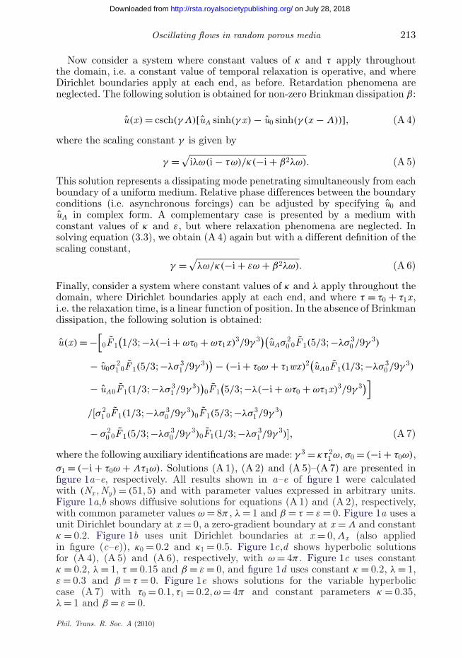
In order to perform the Darcian numerical solution over the unit square, wechoose the following parameter values: Λx = Λy = 1, ω = 6π , β = 0, τ = 0, ε = 0,λ = 1 and κG = 1/3. The spatial discretization is set at (Nx , Ny) = (92, 92), withintegral scale ρ set at two nodal increments ρ = 2Λx/(Nx − 1) ≈ 0.022, with thecorresponding wavenumber kρ = 2π/ρ ≈ 286. Such a small grid will not allow usto perform meaningful calculations of statistical stationarity of the property andsolution fields, but it will provide a convenient test of the performance of theestimator (4.16).

To ensure conformity with the solution (5.1), we apply zero-gradient boundaryconditions on both y edges; on the x = 0 and Λx edges. Unit Dirichlet fluctuationsare imposed (in phase), i.e. u0 = uΛ = 1. Thus, the numerical solution alongany line of constant y will approximate the one-dimensional solution (5.1).It remains to specify the variance σ 2

F to complete the numerical solution. Figure 2presents (a) one realization of F with σ 2

F = 0.5 and (b) its spectral density.The spectral density line was averaged over Nx/2 = 46 randomly chosen transectsthrough the two-dimensional density function, and is compared with the imposedGaussian form shown by the solid line, evaluated using ρ = 2.2Λx/(Nx − 1) andrescaled to match at k = 0. The 10 per cent inaccuracy in integral scale arises





1

S FF

k = kρ

0.01

0.1

0.001

1.0

0.5

0

x

y

x

y

x

y

0 50 100 150k = 2π/Δx

200 250 300

k

|u∧|

|u∧ |

Φ (arg u∧)Φ

(arg

u∧ )

1

0.8

0.6

0.4

0.2

00.2 0.4 0.6

x /Λx x /Λx

0.8 1.0 0 0.2 0.4 0.6 0.8 1.0

0.4

0.6

0.8

1.0

0.2

0 –0.25

0.25

0

Re[

δu∧ ], I

m[δ

u∧ ]

(a) (b)

(c) (d)

(e) ( f )

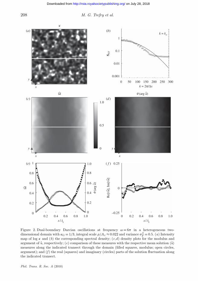
Figure 2. Dual-boundary Darcian oscillations at frequency ω = 6π in a heterogeneous two-dimensional domain with κG = 1/3, integral scale ρ/Λx ≈ 0.022 and variance σ 2

F = 0.5. (a) Intensitymap of log κ and (b) the corresponding spectral density; (c,d) density plots for the modulus andargument of u, respectively; (e) comparison of these measures with the respective mean solution 〈u〉measures along the indicated transect through the domain (filled squares, modulus; open circles,argument); and (f ) the real (squares) and imaginary (circles) parts of the solution fluctuation alongthe indicated transect.





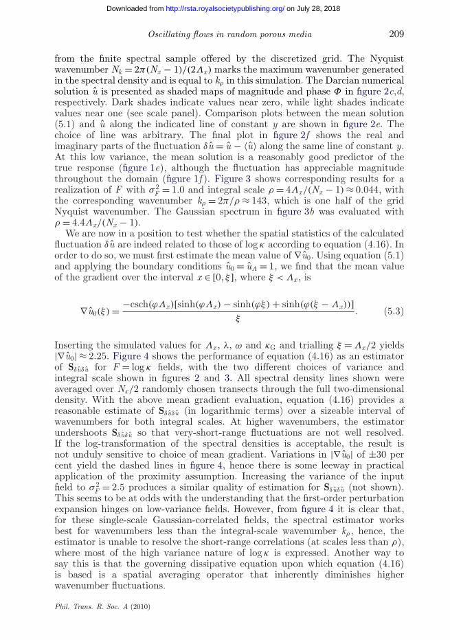
from the finite spectral sample offered by the discretized grid. The Nyquistwavenumber Nk = 2π(Nx − 1)/(2Λx) marks the maximum wavenumber generatedin the spectral density and is equal to kρ in this simulation. The Darcian numericalsolution u is presented as shaded maps of magnitude and phase Φ in figure 2c,d,respectively. Dark shades indicate values near zero, while light shades indicatevalues near one (see scale panel). Comparison plots between the mean solution(5.1) and u along the indicated line of constant y are shown in figure 2e. Thechoice of line was arbitrary. The final plot in figure 2f shows the real andimaginary parts of the fluctuation δu = u − 〈u〉 along the same line of constant y.At this low variance, the mean solution is a reasonably good predictor of thetrue response (figure 1e), although the fluctuation has appreciable magnitudethroughout the domain (figure 1f ). Figure 3 shows corresponding results for arealization of F with σ 2

F = 1.0 and integral scale ρ = 4Λx/(Nx − 1) ≈ 0.044, withthe corresponding wavenumber kρ = 2π/ρ ≈ 143, which is one half of the gridNyquist wavenumber. The Gaussian spectrum in figure 3b was evaluated withρ = 4.4Λx/(Nx − 1).

We are now in a position to test whether the spatial statistics of the calculatedfluctuation δu are indeed related to those of log κ according to equation (4.16). Inorder to do so, we must first estimate the mean value of ∇u0. Using equation (5.1)and applying the boundary conditions u0 = uΛ = 1, we find that the mean valueof the gradient over the interval x ∈ [0, ξ ], where ξ < Λx , is

∇u0(ξ) = −csch(ϕΛx)[sinh(ϕΛx) − sinh(ϕξ) + sinh(ϕ(ξ − Λx))]ξ

. (5.3)

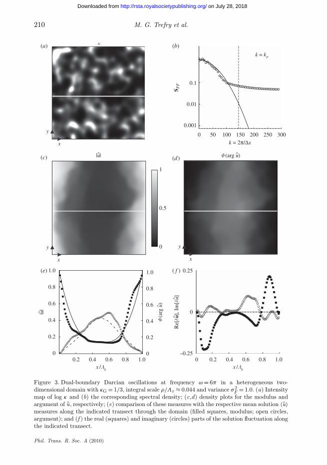
Inserting the simulated values for Λx , λ, ω and κG and trialling ξ = Λx/2 yields|∇u0| ≈ 2.25. Figure 4 shows the performance of equation (4.16) as an estimatorof Sδuδu for F = log κ fields, with the two different choices of variance andintegral scale shown in figures 2 and 3. All spectral density lines shown wereaveraged over Nx/2 randomly chosen transects through the full two-dimensionaldensity. With the above mean gradient evaluation, equation (4.16) provides areasonable estimate of Sδuδu (in logarithmic terms) over a sizeable interval ofwavenumbers for both integral scales. At higher wavenumbers, the estimatorundershoots Sδuδu so that very-short-range fluctuations are not well resolved.If the log-transformation of the spectral densities is acceptable, the result isnot unduly sensitive to choice of mean gradient. Variations in |∇u0| of ±30 percent yield the dashed lines in figure 4, hence there is some leeway in practicalapplication of the proximity assumption. Increasing the variance of the inputfield to σ 2

F = 2.5 produces a similar quality of estimation for Sδuδu (not shown).This seems to be at odds with the understanding that the first-order perturbationexpansion hinges on low-variance fields. However, from figure 4 it is clear that,for these single-scale Gaussian-correlated fields, the spectral estimator worksbest for wavenumbers less than the integral-scale wavenumber kρ , hence, theestimator is unable to resolve the short-range correlations (at scales less than ρ),where most of the high variance nature of log κ is expressed. Another way tosay this is that the governing dissipative equation upon which equation (4.16)is based is a spatial averaging operator that inherently diminishes higherwavenumber fluctuations.





0.1

κ

0.01

0.001

0

x

y

1

0.5

0 y

x

y

x

50 100k = 2π/Δx

150 200 250 300

|u∧|

|u∧ |

1.0

0.8

0.6

0.4

0.2

00.2 0.4 0.6 0.8 1.0 0.20 0.4 0.6 0.8 1.0

0.25

–0.25

0

0.4

0.6

0.8

1.0

0.2

0

Re[

δuu∧ ], I

m[δ

u∧ ]

x /Λxx /Λx

(a) (b)

(c) (d )

(e) ( f )

k = kρ

S FF

Φ (a

rg u∧ )

Φ (arg u∧)

Figure 3. Dual-boundary Darcian oscillations at frequency ω = 6π in a heterogeneous two-dimensional domain with κG = 1/3, integral scale ρ/Λx ≈ 0.044 and variance σ 2

F = 1.0. (a) Intensitymap of log κ and (b) the corresponding spectral density; (c,d) density plots for the modulus andargument of u, respectively; (e) comparison of these measures with the respective mean solution 〈u〉measures along the indicated transect through the domain (filled squares, modulus; open circles,argument); and (f ) the real (squares) and imaginary (circles) parts of the solution fluctuation alongthe indicated transect.





1(a) (b)

10 –2

10 –4

estimatorestimator

k = kρk = kρ

SFF

SFF

Sd u∧

d uu∧

Sd u∧

d uu∧

0 50

spec

tral

den

sity

spec

tral

den

sity

100 150

k = 2p/Δx k = 2p/Δx200 250 300 0 50 100 150 200 250 30010

–6

1

10 –2

10 –4

10 –6

Figure 4. Performance of the forward spectral estimator (4.16, solid curves) for the Darciansolutions of figures 2 and 3 in (a,b), respectively. The dotted curves show the estimators evaluatedwith 30% increase and decrease in the mean gradient constant.

6. Conclusion

This paper has presented governing equations for oscillating flows in porousmedia for the case of a generalized linear fluid constitutive equation thatmodels viscoelastic dissipation and temporal relaxation/retardation processes.Such equations have been shown by other researchers to admit dissipating waveand overshoot phenomena, which may be of interest in the analysis of oscillatingscalar dependent variables (e.g. heat, pressure, concentration) in the regolith.Simple diffusive oscillations can be recovered by appropriate choice of constitutiveparameters. Turbulent processes are not considered. The linearity of the governingequations permits frequency decomposition, so that boundary forcing modes canbe treated separately. A standard finite-difference numerical scheme providedgood solution convergence in both diffusive and standing wave limits of theconstitutive relation.

Most porous media display spatial heterogeneity in their physical, chemicaland biological properties. This property richness means that forward predictionof fluid transport and reaction is problematic unless some basic spatial statisticsof the property fields can be measured or inferred. Here, we have shown that,for cases where the relaxation and retardation terms are small, the spatialspectral density of oscillations in the scalar dependent variable (induced byboundary forcings) can be related to the spatial spectral densities of the porousmedium property fields. This relationship was derived by a first-order stochasticperturbation approach that limits the application of the result to low-varianceproperty fields and to measurements taken close to the forcing boundary. Theusefulness of the spectral relationship was examined for a Darcy flow problemover a randomly heterogeneous permeability field. The spectral relationship wasfound to be a good estimator at low and moderate permeability variances atleast, and was not unduly sensitive to the spatial average of mean gradientsnear the forcing boundaries (a required parameter). Exhaustive testing of the





spectral relationship for heterogeneous relaxation and retardation property fieldsis beyond the scope of this paper, but is relevant to the study of stronglydissipating wave-like phenomena in granular and sedimentary systems.

The value of the spectral relationship derived here is that it is invertiblefor a useful interval of wavenumbers. That is, it may be used to infer spectralcharacteristics of the porous medium property fields over a range of spatial scalesfrom observations of the space–time spectra of the scalar dependent variable. Thepredictive power of the estimator is least in the small- and large-wavenumberlimits, and greatest in wavenumber ranges corresponding to distances of severalcorrelation scales of the input property fields. Typically, in situ observationsof pressure, heat or concentration are inexpensive in comparison to in situmeasurements of porous medium properties, so the inversion offers potentialbenefits in terms of property characterization. However, in order to providerobust estimates of the spatial correlation structure of the problem, it seemsto be necessary to extend the accuracy of the estimator to higher wavenumbers.Furthermore, optimal sampling techniques may need to be considered in order toreduce uncertainty of property estimates based on small numbers of observationsof the scalar dependent variable, which is most likely to be the case inpractical application.

Appendix A. Analytical and numerical solutions

In the following text, we compile some useful analytical solutions to the governingequation (3.3). Consider the diffusive limit β2 = τ = ε = 0 over the finite domainx ∈ [0, Λ], with a Dirichlet condition at the origin, i.e. u(0) = u0, and a Neumanncondition at the upper boundary, i.e. u′(Λ) = u′

Λ. The simple case where κ is aconstant yields

u(x) = sech(ϕΛ)[u0ϕ cosh(ϕ(x − Λ)) + u′Λ sinh(xϕ)]

ϕ, (A 1)

with ϕ ≡ √iλω/κ. The permittivity of the medium is parameterized by the

modulus of ϕΛ: where |ϕΛ| is large (e.g. high frequencies), the migratingdisturbance is rapidly dissipated, and where |ϕΛ| is small (e.g. low frequencies),the migrating disturbance can persist over long distances. For the case κ =κ0 + κ1x and Dirichlet conditions at both ends of the domain u(0) = u0 andu(Λ) = uΛ, equation (3.3) is also soluble, yielding

u(x) =[K0

(2√

iλω(κ0 + κ1x)/κ21

)(u0 0F 1(1; ϕ2

1) − uΛ 0F 1(1; ϕ20)

)

+ (uΛK0(2ϕ0) − u0K0(2ϕ1)

)0F1(1; iλω(κ0 + κ1x)/κ2

1 )]/[K0(2ϕ0)0F1(1; ϕ2

1)

− K0(2ϕ1)0F1(1; ϕ20)], (A 2)

where K0 is the modified Bessel function of the second kind of order zero, 0F 1 isthe regularized confluent hypergeometric function

0F 1(a; z) = 0F 1(a; z)/Γ (a) =∞∑

n=0

zn

Γ (a + n)n! (A 3)

and the auxiliary quantities ϕ0 and ϕ1 are given by√

iκ0λω/κ1 and√i(κ0 + κ1Λ)λω/κ1, respectively.





Now consider a system where constant values of κ and τ apply throughoutthe domain, i.e. a constant value of temporal relaxation is operative, and whereDirichlet boundaries apply at each end, as before. Retardation phenomena areneglected. The following solution is obtained for non-zero Brinkman dissipation β:

u(x) = csch(γΛ)[uΛ sinh(γ x) − u0 sinh(γ (x − Λ))], (A 4)

where the scaling constant γ is given by

γ =√

iλω(i − τω)/κ(−i + β2λω). (A 5)

This solution represents a dissipating mode penetrating simultaneously from eachboundary of a uniform medium. Relative phase differences between the boundaryconditions (i.e. asynchronous forcings) can be adjusted by specifying u0 anduΛ in complex form. A complementary case is presented by a medium withconstant values of κ and ε, but where relaxation phenomena are neglected. Insolving equation (3.3), we obtain (A 4) again but with a different definition of thescaling constant,

γ =√

λω/κ(−i + εω + β2λω). (A 6)

Finally, consider a system where constant values of κ and λ apply throughout thedomain, where Dirichlet boundaries apply at each end, and where τ = τ0 + τ1x ,i.e. the relaxation time, is a linear function of position. In the absence of Brinkmandissipation, the following solution is obtained:

u(x) = −[

0F 1(1/3; −λ(−i + ωτ0 + ωτ1x)3/9γ 3)(uΛσ 2

0 0F 1(5/3; −λσ 30 /9γ 3)

− u0σ21 0F 1(5/3; −λσ 3

1 /9γ 3)) − (−i + τ0ω + τ1wx)2(uΛ0F 1(1/3; −λσ 3

0 /9γ 3)

− uΛ0F 1(1/3; −λσ 31 /9γ 3)

)0F 1

(5/3; −λ(−i + ωτ0 + ωτ1x)3/9γ 3)]

/[σ 21 0F 1(1/3; −λσ 3

0 /9γ 3)0F 1(5/3; −λσ 31 /9γ 3)

− σ 20 0F 1(5/3; −λσ 3

0 /9γ 3)0F1(1/3; −λσ 31 /9γ 3)], (A 7)

where the following auxiliary identifications are made: γ 3 = κτ 21 ω, σ0 = (−i + τ0ω),

σ1 = (−i + τ0ω + Λτ1ω). Solutions (A 1), (A 2) and (A 5)–(A 7) are presented infigure 1a–e, respectively. All results shown in a–e of figure 1 were calculatedwith (Nx , Ny) = (51, 5) and with parameter values expressed in arbitrary units.Figure 1a,b shows diffusive solutions for equations (A 1) and (A 2), respectively,with common parameter values ω = 8π , λ = 1 and β = τ = ε = 0. Figure 1a uses aunit Dirichlet boundary at x = 0, a zero-gradient boundary at x = Λ and constantκ = 0.2. Figure 1b uses unit Dirichlet boundaries at x = 0, Λx (also appliedin figure (c–e)), κ0 = 0.2 and κ1 = 0.5. Figure 1c,d shows hyperbolic solutionsfor (A 4), (A 5) and (A 6), respectively, with ω = 4π . Figure 1c uses constantκ = 0.2, λ = 1, τ = 0.15 and β = ε = 0, and figure 1d uses constant κ = 0.2, λ = 1,ε = 0.3 and β = τ = 0. Figure 1e shows solutions for the variable hyperboliccase (A 7) with τ0 = 0.1, τ1 = 0.2, ω = 4π and constant parameters κ = 0.35,λ = 1 and β = ε = 0.





Direct integration of the generalized governing equation can be achievedvia finite differences as follows. Consider a two-dimensional domain (x , y) ∈[0, Λx ] × [0, Λy], divided into a regular rectangular grid of Nx × Ny nodes, overwhich the numerical solution ui,j is defined (extensions to three dimensions arestraightforward). Coordinate mappings are given by (xi , yj) = ((i − 1)�x , (j −1)�y) for i = 1, 2, . . . , Nx and j = 1, 2, . . . , Ny , with �x = Λx/(Nx − 1) and�y = Λy/(Ny − 1). If we assume that κ is defined and piecewise continuousat all points of the domain, then we arrive at the following derivativediscretizations:

∇ · (κ(xi)∇u(xi , yj)) ≈ 1�x2

[κ−1/2,0u−1,0 − (κ−1/2,0 + κ1/2,0)u0,0 + κ1/2,0u1,0]

+ 1�y2

[κ0,−1/2u0,−1 − (κ0,−1/2 + κ0,1/2)u0,0 + κ0,1/2u0,1](A 8)

and

∇f (xi , yj) ≈(

12�x

(f1,0 − f−1,0),1

2�y(f0,1 − f0,−1)

); f = u, ε, τ . (A 9)

In (A 8) and (A 9), the right-hand sides are expressed in terms of relativecoordinate indices, so that u0,0 = ui,j , u−1,0 = ui−1,j , etc. Assembling all the termsin equation (3.3) yields

1�x2

[κ−1/2,0u−1,0 − (κ−1/2,0 + κ1/2,0)u0,0 + κ1/2,0u1,0]

+ 1�y2

[κ0,−1/2u0,−1 − (κ0,−1/2 + κ0,1/2)u0,0 + κ0,1/2u0,1]

+ ωκ0,0

i − ωτ0,0

[1

4�x2(τ1,0 − τ−1,0)(u1,0 − u−1,0) + 1

4�y2(τ0,1 − τ0,−1)(u0,1 − u0,−1)

]

+ iωκ0,0

1 + iωε0,0 + iωλβ2

[1

4�x2(ε1,0 − ε−1,0)(u1,0 − u−1,0)

+ 14�y2

(ε0,1 − ε0,−1)(u0,1 − u0,−1)

]− λω(i − ωτ0,0)

1 + iωε0,0 + iωλβ2u0,0 = 0. (A 10)

If we view only the nodal values κi,j as being known, then using the normaleffective diffusion result for slabs of differing κ in series (Crank 1975), mid-nodalvalues may be estimated using harmonic means,

2κ−1/2,0

= 1κ−1,0

+ 1κ0,0

;2

κ1/2,0= 1

κ1,0+ 1

κ0,0· · ·. (A 11)

As shown in figure 1, the stencil defined by (A 9) and (A 10) providesuseful accuracy for simple and mildly heterogeneous media. For very highlyheterogeneous media, more sophisticated discretizations are possible (Alcouffeet al. 1981; Shashkov & Steinberg 1996), but are not discussed further here.





References

Alcouffe, R. E., Brandt, A., Dendy Jr, J. E., Painter, J. W. 1981 The multi-grid method forthe diffusion equation with strongly discontinuous coefficients. SIAM J. Sci. Stat. Comput. 2,430–454. (doi:10.1137/0902035)

Alishaev, M. G. & Mirzadjanadze, A. Kh. 1975 For the calculation of delay phenomena in filtrationtheory (in Russian). Izvestya Vuzov, Neft i Gaz 6, 71–74.

Brinkman, H. C. 1947 A calculation of the viscous force exerted by a flowing fluid on a denseswarm of particles. Appl. Sci. Res. A 1, 27–34. (doi:10.1007/BF02120313)

Capuani, F., Frenkel, D. & Lowe, C. P. 2003 Velocity fluctuations and dispersion in a simple porousmedium. Phys. Rev. E 67, 056 306. (doi:10.1103/PhysRevE.67.056306)

Cattaneo, C. 1958 Sur une forme de l’equation de la chaleur eliminant le paradoxe d’unepropagation instantanee. C. R. Acad. Sci. Sér. 1 Math. 247, 431–433.

Chester, M. 1963 Second sound in solids. Phys. Rev. 131, 2013–2015. (doi:10.1103/PhysRev.131.2013)

Compte, A. & Metzler, R. 1997 The generalized Cattaneo equation for the description of anomaloustransport processes. J. Phys. A 30, 7277–7289. (doi:10.1088/0305-4470/30/21/006)

Crank, J. 1975 The mathematics of diffusion, 2nd edn. Oxford, UK: Clarendon Press.Darcy, H. 1856 Les fontaines publiques de la ville de Dijon. Paris, France: Dalmont.Freeze, R. A. 1994 Henry Darcy and the fountains of Dijon. Ground Water 32, 23–30.

(doi:10.1111/j.1745-6584.1994.tb00606.x)Furbish, D. J. 1996 Fluid physics in geology, pp. 386–387. New York, NY: Oxford University Press.Grad, H. 1958 Principles of the kinetic theory of gases. Handbuch der Physik 12, 205–294.Khaled, A.-R. A. & Vafai, K. 2003 The role of porous media in modeling flow and heat

transfer in biological tissues. Int. J. Heat Mass Transfer 46, 4989–5003. (doi:10.1016/S0017-9310(03)00301-6)

Khan, M. & Hayat, T. 2008 Some exact solutions for fractional generalized Burgers’ fluid in a porousspace. Nonlinear Anal.: Real World Appl. 9, 1952–1965. (doi:10.1016/j.nonrwa.2007.06.005)

Khisaeva, Z. F. & Ostoja-Starzewski, M. 2006 Thermoelastic damping in nanomechanicalresonators with finite wave speeds. J. Thermal. Stresses 29, 201–216. (doi:10.1080/01495730500257490)

Khuzhayorov, B. Auriault, J.-L. & Royer, P. 2000 Derivation of macroscopic filtration lawfor transient linear viscoelastic fluid flow in porous media. Int. J. Eng. Sci. 38, 487–504.(doi:10.1016/S0020-7225(99)00048-8)

Kim, M. C., Lee, S. B., Kim, S. & Chung, B. J. 2003 Thermal instability of viscoelastic fluids inporous media. Int. J. Heat Mass Transfer 46, 5065–5072. (doi:10.1016/S0017-9310(03)00363-6)

King, A. C., Needham, D. J., Scott, N. H. 1998 The effects of weak hyperbolicity on the diffusionof heat. Proc. R. Soc. Lond. A 454, 1659–1679. (doi:10.1098/rspa.1998.0225)

Manne, K. K., Hurd, A. J. & Kenkre, V. M. 2000 Nonlinear waves in reaction–diffusion systems:the effect of transport memory. Phys. Rev. E 61, 4177–4184. (doi:10.1103/PhysRevE.61.4177)

Marín, E., Marín-Antuña, J. & Díaz-Arencibia, P. 2002 On the wave treatment of theconduction of heat in photothermal experiments with solids. Eur. J. Phys. 23, 523–532.(doi:10.1088/0143-0807/23/5/309)

Maxwell, J. C. 1867 On the dynamical theory of gases. Phil. Trans. R. Soc. Lond. 157, 49–88.(doi:10.1098/rstl.1867.0004)

Parra, J. O., Ababou, R., Sablik, M. J & Hackert, C. J. 1999 A stochastic wavefield solution of theacoustic wave equation based on the random Fourier–Stieltjes increments. J. Appl. Geophys. 42,81–97. (doi:10.1016/S0926-9851(99)00026-9)

Ruan, F. & McLaughlin, D. 1998 An efficient multivariate random field generator using the fastFourier transform. Adv. Water Resour. 21, 385–399. (doi:10.1016/S0309-1708(96)00064-4)

Scott, J. E., Kenkre, V. M. & Hurd, A. J. 1998 Nonlocal approach to the analysis of the stressdistribution in granular systems. II. Application to experiment. Phys. Rev. E 57, 5850–5857.(doi:10.1103/PhysRevE.57.5850)

Shashkov, M. & Steinberg, S. 1996 Solving diffusion equations with rough coefficients in roughgrids. J. Comput. Phys. 129, 383–405. (doi:10.1006/jcph.1996.0257)



http://dx.doi.org/doi:10.1137/0902035

http://dx.doi.org/doi:10.1007/BF02120313

http://dx.doi.org/doi:10.1103/PhysRevE.67.056306

http://dx.doi.org/doi:10.1103/PhysRev.131.2013

http://dx.doi.org/doi:10.1103/PhysRev.131.2013

http://dx.doi.org/doi:10.1088/0305-4470/30/21/006

http://dx.doi.org/doi:10.1111/j.1745-6584.1994.tb00606.x

http://dx.doi.org/doi:10.1016/S0017-9310(03)00301-6


http://dx.doi.org/doi:10.1016/j.nonrwa.2007.06.005





http://dx.doi.org/doi:10.1098/rspa.1998.0225



http://dx.doi.org/doi:10.1098/rstl.1867.0004




http://dx.doi.org/doi:10.1006/jcph.1996.0257



Shivakumara, I. S. & Sureshkumar, S. 2008 Effects of throughflow and quadratic drag onthe stability of a doubly diffusive Oldroyd-B fluid-saturated porous layer. J. Geophys. Eng.5, 268–280. (doi:10.1088/1742-2132/5/3/003)

Tan, W.-C. 2006 Velocity overshoot of start-up flow for a Maxwell fluid in a porous half-space.Chinese Phys. 15, 2644–2650. (doi:10.1088/1009-1963/15/11/031)

Tan, W. & Masuoka, T. 2005 Stokes’ first problem for an Oldroyd-B fluid in a porous half space.Phys. Fluids 17, 023 101. (doi:10.1063/1.1850409)

Townley, L. R. 1995 The response of aquifers to periodic forcing. Adv. Water Resour. 18, 125–146.(doi:10.1016/0309-1708(95)00008-7)

Wang, S. & Tan, W. 2008 Stability analysis of double-diffusive convection of Maxwell fluidin a porous medium heated from below. Phys. Lett. A 372, 3046–3050. (doi:10.1016/j.physleta.2008.01.024)

Xue, C., Nie, J. & Tan, W. 2008 An exact solution of start-up flow for the fractionalgeneralized Burgers’ fluid in a porous half-space. Nonlinear Anal. 69, 2086–2094. (doi:10.1016/j.na.2007.07.047)





http://dx.doi.org/doi:10.1016/0309-1708(95)00008-7

http://dx.doi.org/doi:10.1016/j.physleta.2008.01.024

http://dx.doi.org/doi:10.1016/j.physleta.2008.01.024

http://dx.doi.org/doi:10.1016/j.na.2007.07.047

http://dx.doi.org/doi:10.1016/j.na.2007.07.047


on oscillating ﬂows in randomly heterogeneous porous...

Documents