On Re-Balancing Self-Interested Agents in Ride-Sourcing Transportation Networks

Armin Sadeghi Stephen L. Smith

Abstract— This paper focuses on the problem of controllingself-interested drivers in ride-sourcing applications. Each driverhas the objective of maximizing its profit, while the ride-sourcing company focuses on customer experience by seeking tominimizing the expected wait time for pick-up. These objectivesare not usually aligned, and the company has no direct controlon the waiting locations of the drivers. In this paper, we providetwo indirect control methods to optimize the set of waitinglocations of the drivers, thereby minimizing the expected waittime of the customers: 1) sharing the location of all drivers witha subset of drivers, and 2) paying the drivers to relocate. Weshow that finding the optimal control for each method is NP-hard and we provide algorithms to find near-optimal control ineach case. We evaluate the performance of the proposed controlmethods on real-world data and show that we can achievebetween 20% to 80% improvement in the expected response.

I. INTRODUCTION

In recent years, ride-sourcing services such as UberX andLyft have emerged as an alternative mode of urban trans-portation. The reduced wait times for pickup of these servicesis the compelling feature compared to the conventional taxiservices [1]. A key factor that affects the response time of theservice is where the drivers wait to respond to the next riderequest. Ride-sourcing companies do not have control overthe position of the drivers as they are self-interested unitsmaximizing their objectives. Therefore, a challenge is toensure the drivers are distributed throughout the city in orderto minimize the expected wait time of the customers. Thismust be done either by providing information to drivers, orthrough incentives (payment) that make relocation attractive.

As a method for both re-balancing and increasing thesupply of drivers, Uber introduced surge pricing in highdemand areas. This reduces the expected response time ofservicing the requests by drawing more drivers to those areas.However, the surge pricing can draw drivers away from lowerdemand areas, resulting in higher wait times in those areasand more imbalance [2], [3].

The problem of servicing requests in ride-sourcing net-works can be divided into two major problems: 1) assignmentof the ride request to the drivers; and 2) re-balancing of thedrivers for future ride requests. In this paper, we focus onthe re-balancing problem for a subset of drivers to serviceride requests that arrive sequentially in an environment. Thedrivers’ motion in the environment is captured as a road-map (i.e., graph), and each ride request arrives at a node ofthe graph according to a known arrival rate (see Figure 1).The drivers are self-interested units maximizing the expectedprofit of their workday. Hence, the ride-sourcing company

This research is partially supported by the Natural Sciences and Engi-neering Research Council of Canada (NSERC).

The authors are with the Department of Electrical and ComputerEngineering, University of Waterloo, Waterloo ON, N2L 3G1 Canada(a6sadegh@uwaterloo.ca; stephen.smith@uwaterloo.ca)

Fig. 1: A set of drivers in the ride-sourcing system and a set oflocations with high probability of ride request arrival.

has no direct control over the waiting locations of the drivers.The objective of the ride-sourcing company is to incentivizethe drivers to relocate to a set of waiting locations thatminimizes the expected wait-time of the customers.

Related Work: The problem of dispatching taxis to serviceride requests has been the subject of extensive research [4],[5], [6], [7]. These studies focus on policies to optimallyassign the ride requests to the taxis. In contrast, we focuson the waiting locations of the drivers that minimize theexpected wait time of the customers. We assume the riderequests are assigned in a first-come-first-serve fashion tothe closest available driver which is the common methodemployed by the ride-sourcing companies [8].

The problem of re-balancing service units in the environ-ment has been studied for various applications. In mobility-on-demand problem (MOD) [9], [10], [11], a group ofvehicles are located at a set of stations. The customers arriveat the stations, hire the vehicles for ride, and then drop thevehicles off at their destination stations. The objective is tobalance the vehicles at the stations to minimize the expectedwait time of the customer. In contrast, we consider thecustomer wait-time as the time between the request arrivaland the pick-up time, which incorporates the distance of theclosest available vehicle to the pick-up location.

The facility location problem [12], [13] and its extensionto the mobile facility location problem (MFL) [14] is theproblem of distributing facilities in a set of locations torespond to the demands arriving at different locations. Theobjective is to minimize the time to respond to the demandsand the total cost of opening facilities. A special case ofthe facility location problem is the k-median problem [13]where the number of open facilities is limited and thecost of opening a facility is zero. In [15], we addresseda multi-stage MFL problem where we relocate a set of

autonomous vehicles to minimize expected response time forfuture requests in a receding horizon manner.

In the aforementioned studies, the actions of service unitsare controlled by a central unit and the objective of theservice units is aligned with the global objective. However,we consider self-interested units maximizing their own profitsuch that the ride-sourcing companies have no direct controlon their decisions. A closely related problem is that ofVoronoi games on graphs [16] where requests arrive on thevertices of a graph and the objective of each self-interestedservice unit is to maximize the number vertices assignedto them. They cast the problem as a game between theservice units prove that the problem of finding the pureNash equilibrium on general graphs is NP-hard. In [17], theauthors provide the best response strategy for each driver andthey approximate Nash equilibria, which can be utilized bythe ride-sourcing companies to incentivize the drivers in away to maximizes a global objective. These studies focus onthe strategies of the self-interested service units, in contrast,we focus on finding the optimal policy for the ride-sourcingcompany to optimally respond to the ride requests.

Contributions: The contributions of this paper are three-fold. First, we formulate the re-balancing problem of self-interested service units. Second, we propose two indirectmethod to relocate the service units to minimize the expectedresponse time and provide algorithms with near-optimalsolutions. Third and finally, we evaluate the performance ofthe control methods on real-world ride-sourcing data.

The paper is organized as follows. In Section II, we for-mulate the problem of minimizing customer wait-time withself-interested service units. In Section III, we provide thefirst indirect control method based on sharing the informationon the location of the drivers. Section IV.I consists of thesecond control method based on incentive pay to relocatethe drivers to desired waiting locations. Finally in Section V,we provide an extensive set of experiments, on real-worldride-sourcing data, characterizing the performance of the twocontrol methods.

II. PROBLEM FORMULATION

Consider a set of m drivers and a set of pick-up and drop-off locations V . Let G = (V,E, c) be a metric graph onvertices V , let E be the set of edges between the locationsand c : E → R+ be the function assigning a travel time toeach edge of the graph. The drivers wait on a subset of thevertices for the next request, which we call the configurationof the drivers Q. The set of all configurations of the driversis denoted by Q. Each driver i is aware of the position of asubset of the drivers Ii ⊆ Q, for instance, each driver maybe aware of the location of the other drivers in its vicinity.

We assume that the requests arrive at each vertex uaccording to an independent Poisson process with arrivalrate λu. Upon a request arrival, the closest driver to thevertex of the request is assigned to service the request.Let pa(u) denote the arrival probability, which is the ratioof number of requests arriving at u to the total numberof requests arriving in a period of time. Let the drop-offprobability pd(dropoff = w|pickup = v) be the probability

that a request with pickup location at vertex v has a drop-offlocation at vertex w.

Driver i’s perception of her expected profit is a functionof her information Ii on the location of other drivers,environment parameters such as arrival times, her waitinglocation qi and the period of working time Bi, denoted byVi(u,Bi). For the development of our main control methodswe do not assume any specific form of this function. We doassume, however, that the ride-sourcing company has accessto this function, obtained through data of driver behavior.In Section V we present one potential model of Vi(u,Bi),which is then used for simulating the two control methods.

Drivers’ objective: Each driver is a self-interested unit,therefore, they will wait at a location that maximizes theirexpected profit, i.e.,

maxu∈V−σc(qi, u) + Vi(u,Bi − c(qi, u)), (1)

where σ is the cost per minute of driving.Global objective: In addition to the objective of each

driver, there is a global objective for the service providersto maximize the service quality by minimizing the expectedwait time of the customers until pick-up, i.e.,

minQ∈Q

D(Q) =∑u∈V

minqi∈Q

pa(u)c(qi, u), (2)

The main challenge in optimizing the global objectiveis that the drivers are self-interested units and the serviceprovider does not have any direct control on the configurationof the vehicles. Therefore, the service provider is not ableto minimize the expected response time to the requestsdirectly. The two indirect control methods proposed in thispaper incentivize the drivers to relocate to desired waitinglocations. The first control method exploits the dependencyof the expected profit of the drivers on their informationIi. The service provider can share more information on thelocation of drivers with a subset of them to manipulate theirdecision towards relocating to a desired waiting location. Werefer to this as the sharing information control. The secondproposed control method, incentivizes the drivers to relocateto desired waiting locations with payments, which we referto as the pay-to-control method. These control methods areapplicable to various models of driver behaviour V .

In the following sections, we provide a detailed descriptionof the two control methods.

III. CONTROL BY SHARING INFORMATION

In this section, we provide an indirect control on theconfiguration of the drivers exploiting the fact that theoptimal waiting location for each driver in Equation (1) is afunction of the information provided to the driver regardingthe position of the other drivers, i.e., Ii.

Figure 2 demonstrates the importance of information on aninstance of the ride-sourcing problem with two vehicles andtwo request locations. The locations are within unit distanceapart and the arrival rate at locations v1 and v2 are 0.1 and0.2, respectively. The vehicles are initially located at v1 andwill relocate to the best waiting location, namely optimizing

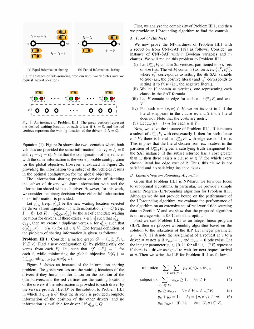
(a) Equal information sharing (b) Partial information sharing

Fig. 2: Instance of ride-sourcing problem with two vehicles and tworequest arrival locations.

Fig. 3: An instance of Problem III.1. The green vertices representthe desired waiting location of each driver if Ii = ∅, and the redvertices represent the waiting location of the drivers if Ii = Q.

Equation (1). Figure 2a shows the two scenarios where bothvehicles are provided the same information, i.e., I1 = I2 = ∅and I1 = I2 = Q. Note that the configuration of the vehicleswith the same information is the worst possible configurationfor the global objective. However, illustrated in Figure 2b,providing the information to a subset of the vehicles resultsin the optimal configuration for the global objective.

The information sharing problem consists of decidingthe subset of drivers we share information with and theinformation shared with each driver. However, for this work,we consider the binary decision where either full informationor no information is provided.

Let q′i,Q (resp. q′i,∅) be the new waiting location selectedby driver i from Equation (1) with information Ii = Q (resp.Ii = ∅). Let Fi = {q′i,Q, q′i,∅} be the set of candidate waitinglocations for driver i. If there exist i, j ∈ [m] such that q′i,Ii =q′j,Ij , then we create a duplicate vertex u for q′j,Ij such thatc(q′i,Ij , v) = c(u, v) for all v ∈ V . The formal definition ofthe problem of sharing information is given as follows:Problem III.1. Consider a metric graph G = (∪mi=1Fi ∪V,E, c). Find a new configuration Q′ by picking only onevertex from each Fi, i.e., such that |Q′ ∩ Fi| = 1 foreach i, while minimizing the global objective D(Q′) =∑u∈V minqi∈Q′ pa(u)c(q, u).Figure 3 shows an instance of the information sharing

problem. The green vertices are the waiting locations of thedrivers if they have no information on the position of theother drivers, and the red vertices are the waiting locationsof the drivers if the information is provided to each driver bythe service provider. Let Q′ be the solution to Problem III.1in which if qi,Q ∈ Q′ then the driver i is provided completeinformation of the position of the other drivers, and noinformation is available for driver i if q′i,∅ ∈ Q

′.

First, we analyze the complexity of Problem III.1, and thenwe provide an LP-rounding algorithm to find the controls.

A. Proof of HardnessWe now prove the NP-hardness of Problem III.1 with

a reduction from CNF-SAT [18] as follows: Consider aninstance of CNF-SAT with n Boolean variables and mclauses. We will reduce this problem to Problem III.1.

(i) Let ∪mi=1Fi contain 2n vertices, partitioned into n setsof size two. The set Fi contains two vertices, {vTi , vFi },where vTi corresponds to setting the ith SAT variableto true (i.e., the positive literal) and vFi corresponds tosetting it to false (i.e., the negative literal).

(ii) We let V contain m vertices, one representing eachclause in the SAT formula.

(iii) Let E contain an edge for each v ∈ ∪mi=1Fi and w ∈V .

(iv) For each e = (v, w) ∈ E, we set its cost to 1 if theliteral v appears in the clause w, and 2 if the literaldoes not. Note that the costs are metric.

(v) Let pa(u) = 1/m for each u ∈ V .Now, we solve the instance of Problem III.1. If it returns

a subset of ∪mi=1Fi with cost exactly 1, then for each clausec ∈ V , there is literal in ∪mi=1Fi with edge cost of 1 to c.This implies that the literal chosen from each subset in thepartition of ∪mi=1Fi gives a satisfying truth assignment forthe SAT instance. If the subset returned has a cost greaterthan 1, then there exists a clause w ∈ V for which everychosen literal has edge cost of 2. Thus, this clause is notsatisfied and no satisfying instance exists.

B. Linear-Program Rounding AlgorithmGiven that Problem III.1 is NP-hard, we turn our focus

to suboptimal algorithms. In particular, we provide a simpleLinear Program (LP)-rounding algorithm for Problem III.1.Although we do not provide bound on the performance ofthe LP-rounding algorithm, we evaluate the performance ofthe algorithm on an extensive set of real-world ride sourcingdata in Section V and we show that the proposed algorithmis on average within 0.014% of the optimal.

First we cast Problem III.1 as an integer linear program(ILP), then we propose a rounding algorithm based on thesolution to the relaxation of the ILP. Let integer parameterxu,v ∈ {0, 1} denote the assignment of a request at v to adriver at vertex u if xu,v = 1, and xu,v = 0 otherwise. Letthe integer parameter yu ∈ {0, 1} for all u ∈ ∪mi Fi representif there is a driver assigned to wait for next request arrivalat u. Then we write the ILP for Problem III.1 as follows:

minimize∑v∈V

∑u∈∪m

i Fi

pa(v)c(u, v)xu,v (3)

subject to:∑

u∈∪mi Fi

xu,v ≥ 1, ∀v ∈ V (4)

yu ≥ xu,v, ∀v ∈ V, u ∈ ∪mi Fi (5)yu + yv = 1, Fi = {u, v}, i ∈ [m] (6)yu, xu,v ∈ {0, 1}, ∀v ∈ V, u ∪mi Fi

By constraint (4), a feasible solution assigns each requestlocation to a driver. Equation (5) ensures that a request isassigned to u only if there is a driver located at u, and finallyEquation (6) shows that in a feasible solution only one ofthe candidate waiting locations is chosen from each subsetFi, which represent that either the information is providedto a driver or otherwise.

Now we propose our LP-rounding algorithm for Prob-lem III.1. Let (x′,y′) be the solution to the LP relaxation ofILP (3). Without loss of generality for all Fi = {u, v}, i ∈[m], let yu ≥ 1/2 and yv ≤ 1/2. Given solution (x′,y′) weconstruct an integer solution to ILP (3) by setting yu = 1for each vertex u with y′u > 1/2 and yv = 0. In a case,Fi = {u, v} and y′u = y′v = 1/2, we set yu = 1 where u isthe optimal waiting location of driver i with Ii = ∅. Then weassign each vertex v ∈ V to the closest vertex u in ∪mi=1Fiwith yu = 1 by setting xu,v = 1. Note that the constructedsolution (x, y) satisfies the constraint of ILP (3), therefore,it is a feasible solution to Problem III.1. Also, observe thatthe optimal objective value to the LP relaxation is a lower-bound on the optimal value of ILP (3) and provides a boundon the performance of the LP-rounding algorithm.

In the solution to the information sharing problem, if driveri is selected to receive information on the location of drivers,a snapshot of the location of drivers is presented to driveri and the driver can calculate their expected profit basedon complete information. This method employed at eachtime step and presents information to a driver if there isan opportunity to improve the expected response time.

The information sharing method indirectly controls theconfiguration of the drivers by providing information to asubset of them, however, the possible configurations arelimited to the candidate waiting locations of the drivers. Inthe following section, we provide the details on the pay-to-control method for the service provider.

IV. PAY TO CONTROL

Each driver as a self-interested unit chooses its waiting lo-cation by maximizing the profit in Equation (1). To convincethe vehicles to relocate to another configuration, the serviceprovider needs to compensate for the difference between theirexpected profit of the new location and their expected profitfor the waiting location from Equation (1). First, we pose theproblem between the drivers and the service provider as agame. Then we provide an approximation algorithm to findthe optimal policy for the service provider.

A. Service Provider’s Game

Let di be the incentive per unit distance offered to driveri. Let Q = {q1, . . . , qm} (resp. Q′ = {q′1, . . . , q′m}) be theconfiguration of the drivers before (resp. after) the incentivepay. The game between the drivers and service providerconsists of the following:• A set of m players and a service provider,• An action set Ai for each driver i, which is the waiting

locations in the graph, i.e. Ai = V ∀i ∈ [m]. The actionset of the service provider is Q; and

• The profit function of the service provider is h(Q′) =∑i∈m diσc(qi, q

′i) + βD(Q′), where β ≥ 0 is a user-

defined parameter that indicates the importance of theservice quality for the service provider with respect tothe incentive pay. For a small value of β, the incentivepay is in the priority, thus the service provider willoffer the waiting locations close to the drivers’ desiredwaiting locations, however, for large values of β, theservice provider accepts high incentive pay to relocatethe drivers to a configuration with minimum expectedresponse time.

• The profit of driver i is the maximum of the expectedprofit of the offered waiting location with incentive payand the expected profit of the waiting location fromEquation (1), i.e.,

max{(di − 1)σc(qi, q′i) + V(q′i, Bi − c(qi, q′i)),

maxu∈V−σc(qi, u) + V(u,Bi − c(qi, u))}. (7)

This is an instance of a leader-follower game [19]. Theservice provider offers an incentive based on its utility andthe drivers as followers either take the offer or reject it.The service provider is aware of the best action of thedrivers given any action taken by the service provider (i.e.,incentive pay and the offered waiting location). The objectiveis to find the optimal strategy for the service provider tominimize a linear combination of the incentive pay andthe expected response time by relocating the drivers to thedesired configuration.

Driver i will accept the offer by the service provider torelocate to q′i only if the offered incentives surpass the best-expected profit of the driver. Since the profit functions of thedrivers are known to the service provider, then the minimumdi in which the drivers will accept the offer to move toconfiguration Q′ is

di =maxu∈V −σc(qi, u) + Vi(u,B − c(qi, u))

c(qi, q′i)

− Vi(q′i, Bi − c(qi, q′i))σc(qi, q′i)

+ 1. (8)

In the equation above, maxu∈V −σc(qi, u) + Vi(u,B −c(qi, u)) is the maximum expected profit of the driver i byrelocating to a new waiting location, and Vi(q′i, Bi−c(qi, q′i))is the expected profit of driver i by waiting at the locationq′i offered by the service provider. Knowing this minimumdi, the objective of the service provider becomes

h(Q′) =∑i∈m

σc(qi, q′i) + β

∑u∈V

pu mini∈[m]

c(q′i, u)

+∑i∈m

maxu∈V−σc(qi, u) + Vi(u,B − c(qi, u))

−∑i∈mVi(q′i, Bi − c(qi, q′i)). (9)

Observe that∑i∈m maxu∈V −σc(qi, u)+Vi(u,B−c(qi, u))

is independent of the optimization parameters. Therefore, theproblem of minimizing the utility function of the serviceprovider h has the mobile facility location (MFL) problem

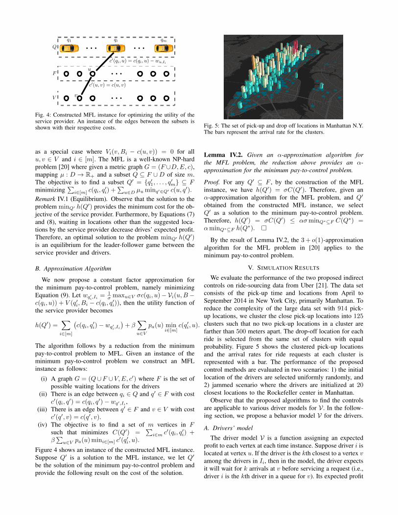
Fig. 4: Constructed MFL instance for optimizing the utility of theservice provider. An instance of the edges between the subsets isshown with their respective costs.

as a special case where Vi(v,Bi − c(u, v)) = 0 for allu, v ∈ V and i ∈ [m]. The MFL is a well-known NP-hardproblem [20] where given a metric graph G = (F ∪D,E, c),mapping µ : D → R+ and a subset Q ⊆ F ∪D of size m.The objective is to find a subset Q′ = {q′1, . . . , q′m} ⊆ Fminimizing

∑i∈[m] c(qi, q

′i) +

∑u∈D µu minq′∈Q′ c(u, q

′).

Remark IV.1 (Equilibrium). Observe that the solution to theproblem minQ′ h(Q′) provides the minimum cost for the ob-jective of the service provider. Furthermore, by Equations (7)and (8), waiting in locations other than the suggested loca-tions by the service provider decrease drives’ expected profit.Therefore, an optimal solution to the problem minQ′ h(Q′)is an equilibrium for the leader-follower game between theservice provider and drivers.

B. Approximation Algorithm

We now propose a constant factor approximation forthe minimum pay-to-control problem, namely minimizingEquation (9). Let wq′i,Ii = 1

σ maxu∈V σc(qi, u)−Vi(u,B −c(qi, u)) + V (q′i, Bi − c(qi, q′i)), then the utility function ofthe service provider becomes

h(Q′) =∑i∈[m]

(c(qi, q

′i)− wq′i,Ii

)+ β

∑u∈V

pa(u) mini∈[m]

c(q′i, u).

The algorithm follows by a reduction from the minimumpay-to-control problem to MFL. Given an instance of theminimum pay-to-control problem we construct an MFLinstance as follows:

(i) A graph G = (Q∪F ∪V,E, c′) where F is the set ofpossible waiting locations for the drivers

(ii) There is an edge between qi ∈ Q and q′ ∈ F with costc′(qi, q

′) = c(qi, q′)− wq′,Ii ,

(iii) There is an edge between q′ ∈ F and v ∈ V with costc′(q′, v) = c(q′, v).

(iv) The objective is to find a set of m vertices in Fsuch that minimizes C(Q′) =

∑i∈m c

′(qi, q′i) +

β∑u∈V pa(u) mini∈[m] c

′(q′i, u).

Figure 4 shows an instance of the constructed MFL instance.Suppose Q′ is a solution to the MFL instance, we let Q′

be the solution of the minimum pay-to-control problem andprovide the following result on the cost of the solution.

Fig. 5: The set of pick-up and drop off locations in Manhattan N.Y.The bars represent the arrival rate for the clusters.

Lemma IV.2. Given an α-approximation algorithm forthe MFL problem, the reduction above provides an α-approximation for the minimum pay-to-control problem.

Proof. For any Q′ ⊆ F , by the construction of the MFLinstance, we have h(Q′) = σC(Q′). Therefore, given anα-approximation algorithm for the MFL problem, and Q′

obtained from the constructed MFL instance, we selectQ′ as a solution to the minimum pay-to-control problem.Therefore, h(Q′) = σC(Q′) ≤ ασminQ∗⊆F C(Q∗) =αminQ∗⊆F h(Q∗).

By the result of Lemma IV.2, the 3 + o(1)-approximationalgorithm for the MFL problem in [20] applies to theminimum pay-to-control problem.

V. SIMULATION RESULTS

We evaluate the performance of the two proposed indirectcontrols on ride-sourcing data from Uber [21]. The data setconsists of the pick-up time and locations from April toSeptember 2014 in New York City, primarily Manhattan. Toreduce the complexity of the large data set with 914 pick-up locations, we cluster the close pick-up locations into 125clusters such that no two pick-up locations in a cluster arefarther than 500 meters apart. The drop-off location for eachride is selected from the same set of clusters with equalprobability. Figure 5 shows the clustered pick-up locationsand the arrival rates for ride requests at each cluster isrepresented with a bar. The performance of the proposedcontrol methods are evaluated in two scenarios: 1) the initiallocation of the drivers are selected uniformly randomly, and2) jammed scenario where the drivers are initialized at 20closest locations to the Rockefeller center in Manhattan.

Observe that the proposed algorithms to find the controlsare applicable to various driver models for V . In the follow-ing section, we propose a behavior model V for the drivers.

A. Drivers’ model

The driver model V is a function assigning an expectedprofit to each vertex at each time instance. Suppose driver i islocated at vertex u. If the driver is the kth closest to a vertex vamong the drivers in Ii, then in the model, the driver expectsit will wait for k arrivals at v before servicing a request (i.e.,driver i is the kth driver in a queue for v). Its expected profit

5 10 15 20 25 30Number of Vehicles

0

5

10

15

20

25P

erce

ntag

eIm

pro

vem

ent

inR

esp

onse

Tim

eRandom initial configuration

Jammed scenario

Fig. 6: Improved expected response time via the information sharingcontrol.

is then calculated by probabilistically considering whichqueue it will reach the front of first, and the expected profitwhen servicing a ride at that vertex along with the expectedfuture profit from that ride’s dropoff location. Due to spaceconstraints, we omit a detailed description of the drivermodel and refer the reader to the extended version of thispaper [22], which contains all further details.

B. Partial Information Sharing

Figure 6 shows the percentage improvement in the ex-pected response time for different number of vehicles usingthe partial information sharing control method of Section IIIin the two scenarios. Observe that as the number of driversincreases, the average improvement in the expected responsetime increases. However, with a large number of driversrandomly placed in the environment, the expected responsetime decreases and the possibility to further optimize it withinformation sharing is limited. On the other hand, in thejammed scenario where the drivers are concentrated in anarea, the information sharing method improves the expectedresponse time by 10% on average. The information sharingmethod shares information on the position of the otherdrivers with 31.0% and 41.7% of the drivers in the randominitial configuration and jammed scenarios, respectively. Theresults are the average of 1000 instances for different numberof drivers and scenarios. The boxes show the first, first andthird quartiles of each set of experiments. The expectedresponse time of the solution obtained from the LP-roundingalgorithm of Section III on this set of experiments is within0.014% on average of the solution of the LP relaxation of theinformation sharing problem. The maximum deviation fromthe optimal solution of the LP relaxation is 0.42%.

Figure 7 shows the expected response time of 20 driversresponding to 100 requests arriving over time with thejammed initial configuration. In this experiment, the maxi-mum arrival rate on the vertices is 0.03 per minute, therefore,we assumed that there exist enough time to relocate betweenthe ride request arrivals. Note that the information sharingmethod maintains a low expected response time over thecourse of responding to 100 requests compared to the sameset of drivers with no control on their waiting locations. Theresults are the average of 100 experiments with 100 random

0 20 40 60 80 100Number of Requests

350

400

450

500

550

600

650

Exp

ecte

dR

esp

onse

Tim

e

Partial Information Share

No control

Fig. 7: The expected response time of a system of 20 driversexecuting 100 ride requests arriving over time. The drivers areinitialized under the jammed scenario.

10 20 30 40Number of Drivers

0

5

10

15

20

25

30

35

Per

centa

geIm

pro

vem

ent

inR

esp

onse

Tim

e

β = 1.0

β = 10.0

10

20

30

40

50

60

Am

ount

Pai

dto

Dri

vers

($)

Fig. 8: The percentage improvement in expected response time andthe incentive pay. The solid lines represent the average improvementin the expected response time and the dashed lines represent thetotal amount paid to the drivers.

requests for each experiment. The lines represent the averageand shaded areas represent the first and third quartiles.

C. Pay to Control

In this section, we evaluate the performance of the PAY-TO-CONTROL method for the two scenarios. Figure 8 il-lustrates the improvement in the expected response (solidlines) time and the total amount paid to the drivers (dashedlines) to relocate for different β values in the random initialconfiguration scenario. The shaded area represents the firstand third quartiles of 1000 random instances for each numberof vehicles. The amount paid is proportional to the averagecost of riding UberXL, i.e., $0.3 per minute [23]. For largerβ, the expected response time is more important than theamount paid for relocation. Therefore, with a larger numberof vehicles, the PAY-TO-CONTROL method increases theamount paid to the drivers to minimize the expected responsetime. Notice that with β = 10 the expected response timehas improved by 25% for $1 per driver.

Next, we evaluate the performance of the pay-to-controlalgorithm in the jammed scenario. Figure 9 shows that witha larger number of vehicles concentrated in a small area,

10 20 30 40Number of Drivers

0

10

20

30

40

50

60

70

80P

erce

nta

geIm

pro

vem

ent

inR

esp

onse

Tim

e

β = 1.0

β = 10.0

20

40

60

80

Am

ount

Pai

dto

Dri

vers

($)

Fig. 9: The percentage improvement in the expected response timeand the incentive pay in the jammed scenario. The solid linesrepresent the average improvement in the expected response timeand the dashed lines represent the total amount paid to the drivers.

0 20 40 60 80 100Number of Requests

300

400

500

600

700

Exp

ecte

dR

esp

onse

Tim

e

Pay-to-Control

No control

Paid amount

0

5

10

15

20

Am

ount

Pai

dto

Dri

vers

($)

Fig. 10: The expected response time and the paid amount to 20drivers, initialized under the jammed scenario, servicing 100 riderequests arriving over time under the PAY-TO-CONTROL method.

the pay-to-control algorithm improves the expected responsetime significantly with limited amounts paid to the drivers.Notice that with β = 10 the expected response time hasimproved by 70% for $2 per driver.

Figure 10 shows the expected response time and theamount paid to a set of 20 drivers responding to 100 requestsarriving over time with the jammed initial configuration.Notice that the PAY-TO-CONTROL method with β = 1maintains a low expected response time over the course ofresponding to 100 requests compared to the same set ofdrivers with no control input on their waiting locations. Thetotal amount paid to the drivers over the course of respondingto 100 requests is $1.87 per request. The results are anaverage of 100 experiments with 100 randomly generatedrequests for each experiment. The lines represent the averageand shaded areas represent the first and third quartiles.

VI. CONCLUSION

This paper considered the problem of controlling self-interested drivers in ride-sourcing applications. Two indirectcontrol methods were proposed and for each, a near-optimalalgorithm was presented. The extensive results show signif-icant improvement in the expected response time on real-

world ride-sourcing data. In addition, we hope to extend theresults to capture vehicles with different capacities and ride-sharing applications.

REFERENCES

[1] L. Rayle, S. Shaheen, N. Chan, D. Dai, and R. Cervero, “App-based, on-demand ride services: Comparing taxi and ridesourcingtrips and user characteristics in san francisco university of californiatransportation center (uctc),” University of California, Berkeley, 2014.

[2] N. Diakopoulos. How Uber surge pricing really works. [Online].Available: https://www.washingtonpost.com/news/wonk/wp/2015/04/17/how-uber-surge-pricing-really-works/

[3] A. Rosenblat and L. Stark, “Algorithmic labor and information asym-metries: A case study of Ubers drivers,” International Journal OfCommunication, 2016.

[4] W. Zhang, S. Guhathakurta, J. Fang, and G. Zhang, “The performanceand benefits of a shared autonomous vehicles based dynamic rideshar-ing system: An agent-based simulation approach,” in TransportationResearch Board 94th Annual Meeting, no. 15-2919, 2015.

[5] M. Hyland and H. S. Mahmassani, “Dynamic autonomous vehicle fleetoperations: Optimization-based strategies to assign AVs to immediatetraveler demand requests,” Transportation Research Part C: EmergingTechnologies, vol. 92, pp. 278–297, 2018.

[6] M. Chang, D. S. Hochbaum, Q. Spaen, and M. Velednitsky, “DIS-PATCH: an optimal algorithm for online perfect bipartite matchingwith i.i.d. arrivals,” CoRR, vol. abs/1805.02014, 2018.

[7] M. Maciejewski, J. Bischoff, and K. Nagel, “An assignment-basedapproach to efficient real-time city-scale taxi dispatching,” IEEEIntelligent Systems, vol. 31, no. 1, pp. 68–77, 2016.

[8] Uber. Driving with Uber, wait less, earn more. [Online]. Available:https://www.uber.com/info/get-trips-without-waiting/

[9] M. Pavone, S. L. Smith, E. Frazzoli, and D. Rus, “Robotic loadbalancing for mobility-on-demand systems,” The International Journalof Robotics Research, vol. 31, no. 7, pp. 839–854, 2012.

[10] M. Tsao, R. Iglesias, and M. Pavone, “Stochastic model predic-tive control for autonomous mobility on demand,” arXiv preprintarXiv:1804.11074, 2018.

[11] G. C. Calafiore, C. Novara, F. Portigliotti, and A. Rizzo, “A flowoptimization approach for the rebalancing of mobility on demandsystems,” in IEEE International Conference on Decision and Control,2017, pp. 5684–5689.

[12] D. B. Shmoys, “Approximation algorithms for facility location prob-lems,” in International Workshop on Approximation Algorithms forCombinatorial Optimization. Springer, 2000, pp. 27–32.

[13] V. Arya, N. Garg, R. Khandekar, A. Meyerson, K. Munagala, andV. Pandit, “Local search heuristics for k-median and facility locationproblems,” SIAM Journal on computing, vol. 33, no. 3, pp. 544–562,2004.

[14] E. D. Demaine, M. Hajiaghayi, H. Mahini, A. S. Sayedi-Roshkhar,S. Oveisgharan, and M. Zadimoghaddam, “Minimizing movement,”ACM Transactions on Algorithms (TALG), vol. 5, no. 3, p. 30, 2009.

[15] A. Sadeghi and S. L. Smith, “Re-deployment algorithms for multipleservice robots to optimize task response,” in IEEE InternationalConference on Robotics and Automation, 2018, pp. 2356–2363.

[16] S. Bandyapadhyay, A. Banik, S. Das, and H. Sarkar, “Voronoi game ongraphs,” Theoretical Computer Science, vol. 562, pp. 270–282, 2015.

[17] R. Salhab, J. Le Ny, and R. P. Malhame, “A dynamic ride-sourcinggame with many drivers,” in 55th Annual Allerton Conference onCommunication, Control, and Computing, 2017, pp. 770–775.

[18] R. Schuler, “An algorithm for the satisfiability problem of formulas inconjunctive normal form,” Journal of Algorithms, vol. 54, no. 1, pp.40–44, 2005.

[19] T. Basar and G. J. Olsder, Dynamic noncooperative game theory.Siam, 1999, vol. 23.

[20] S. Ahmadian, Z. Friggstad, and C. Swamy, “Local-search basedapproximation algorithms for mobile facility location problems,” inProceedings of the twenty-fourth annual ACM-SIAM symposium onDiscrete algorithms. SIAM, 2013, pp. 1607–1621.

[21] (2014) Uber TLC FOIL response. [Online]. Available: https://github.com/fivethirtyeight/uber-tlc-foil-response

[22] A. Sadeghi and S. L. Smith, “On re-balancing self-interestedagents in ride-sourcing transportation networks,” arXiv preprintarXiv:1909.04615, 2019.

[23] Ride sharing driver. How much does uber cost? Uber fare estimator.[Online]. Available: https://www.ridesharingdriver.com/