On relation between mid-latitude ionospheric ionization and quasi-trapped

energetic electrons during 15 December 2006 magnetic storm

A.V. Suvorovaa,b*, L.-C. Tsaia, A.V. Dmitrievc,a

a Center for Space and Remote Sensing Research, National Central University, Jhongli,

Taiwan

b Skobeltsyn Institute of Nuclear Physics Moscow State University, Moscow, Russia

c Institute of Space Science, National Central University, Jhongli, Taiwan

____________________________________________________________________

Abstract

We report simultaneous observations of intense fluxes of quasi-trapped energetic electrons

and substantial enhancements of ionospheric electron concentration (EC) at low and middle

latitudes over Pacific region during geomagnetic storm on 15 December 2006. Electrons with

energy of tens of keV were measured at altitude of ~800 to 900 km by POES and DMSP

satellites. Experimental data from COSMIC/FS3 satellites and global network of ground-

based GPS receivers were used to determine height profiles of EC and vertical total EC,

respectively. A good spatial and temporal correlation between the electron fluxes and EC

enhancements was found. This fact allows us to suggest that the quasi-trapped energetic

electrons can be an important source of ionospheric ionization at middle latitudes during

magnetic storms.

Keywords: ionospheric storms, radiation belts, magnetic storms

____________________________________________________________________

1

1. Introduction 1

2

3

4

5

6

7

8

9

10

11

12

13

14

15

16

17

18

19

20

21

22

23

24

25

Storm-time dynamics of total electron content (TEC), the integral with height of the

ionospheric electron density profile, was studied comprehensively from auroral to equatorial

latitudes for many decades (e.g. Mendillo, 2006). Nowadays, numerous studies concern with

an unresolved problem of TEC enhancements, so-called positive ionospheric storms (e.g.,

Mendillo et al., 2010; Balan et al., 2010; Wei et al., 2011). Complex mechanism of

thermosphere-ionosphere system response to a geomagnetic storm involves a number of

different agents such as disturbance electric fields, changes in neutral winds system and

neutral chemical composition, gravity waves and diffusion. However, it is very difficult to

pick out the agents forming the positive ionospheric storms.

Because of its high conductivity, the ionosphere responses quickly to variations of electric

field due to such effects as magnetospheric convection, ionospheric dynamo disturbance and

various kinds of wave disturbances (e.g., Biktash, 2004). Balan et al. (2011) discuss an

importance of thermospheric storms developing simultaneously with ionospheric ones.

Relative role of prompt penetrating (under-shielded) electric field (PPEF) and equatorward

neutral winds as two sources of positive ionospheric storms at low and middle latitudes is

intensively discussed in literature (Lei et al., 2008; Pedatella et al., 2009; Mendillo et al.,

2010; Balan et al., 2010). Possible errors in the models are attributed to under-representation

of conditions at lower altitudes, variability of the neutral wind and/or coupling with auroral

sources.

Recent studies and models of the ionospheric disturbances observed during a strong

geomagnetic storm on 14-15 December 2006 have revealed that the PPEF and equatorward

neutral winds alone can not explain a long-lasting intense positive ionospheric storm occurred

over Pacific sector during maximum and recovery phase of the magnetic storm (Lei et al.,

2008; Pedatella et al., 2009). Lei et al. (2008) showed that the CMIT model simulations were

2

26

27

28

29

30

31

32

33

34

35

36

37

38

39

40

41

42

43

44

45

46

47

48

49

able to capture the positive storm effect at equatorial ionization anomaly (EIA) crest regions

during 00-03 UT on December 15. On the other hand, the authors pointed out that the model

was unable to reproduce the positive effects observed for several hours after 03 UT. In

addition, the CMIT simulation predicted a depletion of plasma densities over the low-latitude

region at 0000 to 0300 UT on 15 December that is inconsistent with the observations.

Pedatella et al. (2009) reported that during this time the height of F-layer peak increased by

greater than 100 km. It was assumed that the TEC increases, observed in the topside

ionosphere/plasmasphere at middle to high latitudes, might be explained by effects of particle

precipitation. However, experimental evidence of this assumption was not reported.

Here we analyze fluxes of energetic electrons observed by low-altitude (heights ~ 800 to 900

km) satellites of POES and DMSP fleets during magnetic storm on 15 December 2006. We

demonstrate a good correlation of the mid-latitude ionospheric ionization enhancements

observed over Pacific region with the intense fluxes of quasi-trapped energetic electrons.

2. Positive ionospheric storm

A geomagnetic storm started at about 14 UT on 14 December 2006, when a CME-driven

interplanetary shock (IS) affected the Earth’s magnetosphere. The storm initial phase was

lasting until ~2330 UT. After that the CME-related main phase of severe geomagnetic storm

began. The storm maximum with Dst ~ -150 nT and Kp ~ 8+ was observed after midnight of

15 December. The recovery phase started at ~ 08 UT on 15 December. The storm main and

recovery phases were accompanied by a long-lasting (from 00 to 14 UT) and widely

expanded (from 12 to 24 LT) strong positive ionospheric storm with the ionization enhanced

up to 50 TECU (1TECU = 1012 electrons/cm2) over Pacific and American regions (from 120°

to 300° longitude) (Lei et al., 2008; Pedatella et al., 2009).

3

50

51

52

53

54

55

56

57

58

59

60

61

62

63

64

65

66

67

68

69

70

71

72

73

74

One of very important factors in the study of storm-time disturbances is a consistent choice of

quiet-time period. Previous studies of this event used moderately disturbed day on December

13 as a day of “quiet conditions”. We use a day on December 3 when the solar and

geomagnetic activity was very quiet. This choice allows revealing prominent positive

ionospheric storms on the initial, main and recovery phases of the geomagnetic storm. Figure

1 demonstrates development of strong enhancement of vertical TEC (VTEC) at 00 to 06 UT

on 15 December. Global ionospheric maps (GIM) of VTEC are provided every 2 hours by a

world-wide network of ground-based GPS receivers. The residual VTEC (dVTEC) was

calculated as a difference between the disturbed and quiet days.

The positive storms in VTEC tend to occur in the postnoon and dusk sectors above Pacific

and American region. We can distinguish two branches of the VTEC enhancements at low

(~10° to 20° deg) and middle (~30° to 40°) latitudes. The low-latitude positive storm is

oriented strictly along the geomagnetic equator at geomagnetic latitudes of ~15°. This storm

is mostly pronounced and can be explained in the frame of a continuous complex effect of

daytime eastward PPEF and equatorward neutral wind (Balan et al., 2010). The positive

storm at middle latitudes persists within first 6 hours and then diminishes fast after ~06 UT. It

seems that the maximum of mid-latitude storm is slightly moving pole-ward from ~30° to 40°

of geomagnetic latitude. There is no clear explanation of this positive storm.

Vertical profiles of electron concentration (EC) were measured in COSMIC/FS3 space-borne

experiment. The EC is expressed as a number of electrons per cubic centimeter (cc). Six

satellites of the COSMIC/FS3 mission produce a sounding of the ionosphere on the base of

radio occultation (RO) technique, which makes use of radio signals transmitted by the GPS

satellites (Hajj et al., 2000). Usually over 2500 soundings per day provide EC height profiles

over ocean and land. A 3-D EC distribution is deduced through relaxation using red-black

smoothing on numerous EC height profiles. This 3-D EC image is used as an initial guess to

4

75

76

77

78

79

80

81

82

83

84

85

86

87

88

89

90

91

92

93

94

95

96

97

98

99

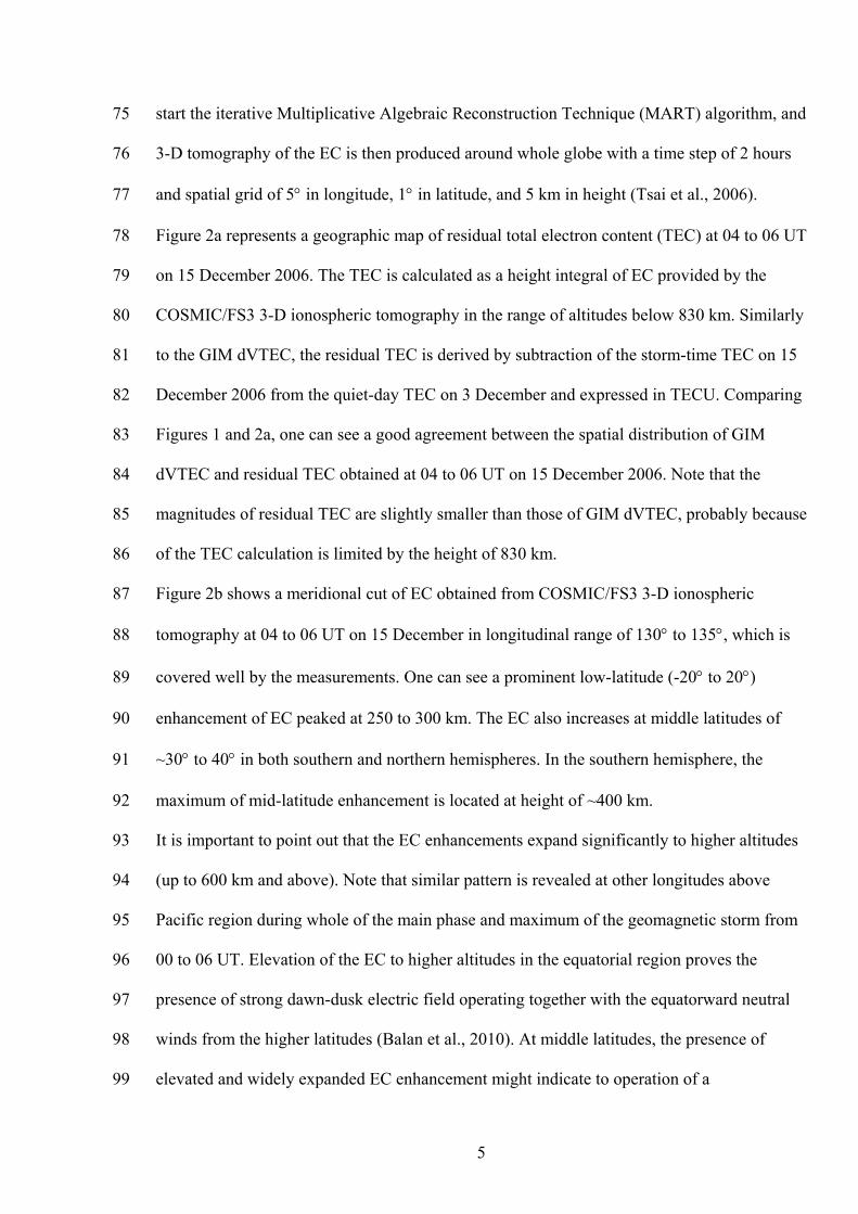
start the iterative Multiplicative Algebraic Reconstruction Technique (MART) algorithm, and

3-D tomography of the EC is then produced around whole globe with a time step of 2 hours

and spatial grid of 5° in longitude, 1° in latitude, and 5 km in height (Tsai et al., 2006).

Figure 2a represents a geographic map of residual total electron content (TEC) at 04 to 06 UT

on 15 December 2006. The TEC is calculated as a height integral of EC provided by the

COSMIC/FS3 3-D ionospheric tomography in the range of altitudes below 830 km. Similarly

to the GIM dVTEC, the residual TEC is derived by subtraction of the storm-time TEC on 15

December 2006 from the quiet-day TEC on 3 December and expressed in TECU. Comparing

Figures 1 and 2a, one can see a good agreement between the spatial distribution of GIM

dVTEC and residual TEC obtained at 04 to 06 UT on 15 December 2006. Note that the

magnitudes of residual TEC are slightly smaller than those of GIM dVTEC, probably because

of the TEC calculation is limited by the height of 830 km.

Figure 2b shows a meridional cut of EC obtained from COSMIC/FS3 3-D ionospheric

tomography at 04 to 06 UT on 15 December in longitudinal range of 130° to 135°, which is

covered well by the measurements. One can see a prominent low-latitude (-20° to 20°)

enhancement of EC peaked at 250 to 300 km. The EC also increases at middle latitudes of

~30° to 40° in both southern and northern hemispheres. In the southern hemisphere, the

maximum of mid-latitude enhancement is located at height of ~400 km.

It is important to point out that the EC enhancements expand significantly to higher altitudes

(up to 600 km and above). Note that similar pattern is revealed at other longitudes above

Pacific region during whole of the main phase and maximum of the geomagnetic storm from

00 to 06 UT. Elevation of the EC to higher altitudes in the equatorial region proves the

presence of strong dawn-dusk electric field operating together with the equatorward neutral

winds from the higher latitudes (Balan et al., 2010). At middle latitudes, the presence of

elevated and widely expanded EC enhancement might indicate to operation of a

5

100

101

102

103

104

105

106

107

108

109

110

111

112

113

114

115

116

117

118

119

120

121

122

magnetospheric mechanism of charged particle contribution to redundant ionization of the

mid-latitude ionosphere.

3. Quasi-trapped electrons

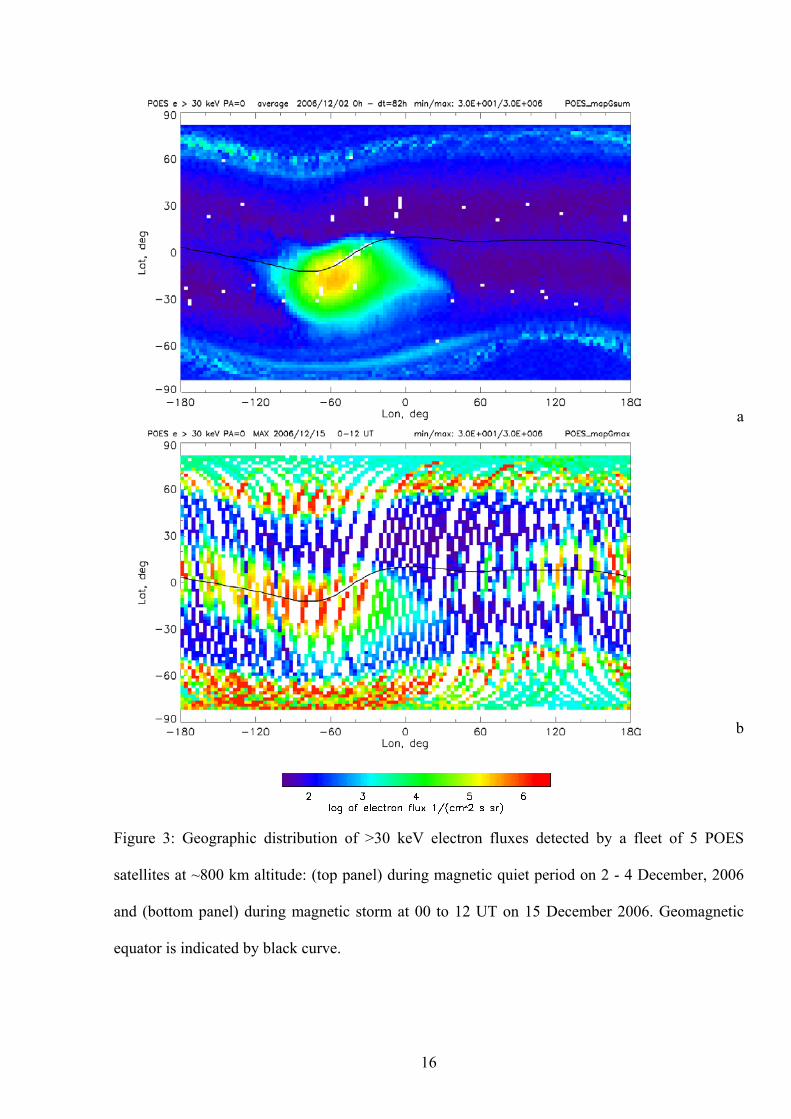
Figure 3 demonstrates geographic distribution of >30 keV electron fluxes observed during

magnetically quiet interval and during magnetic storm on 14-15 December 2006. The

electrons are measured at altitude of 800 km by a fleet of 5 POES satellites (Huston and

Pfitzer, 1998; Evans and Greer, 2004). During magnetic quiet (Figure 3a), the vast majority

of electron population at low altitudes is trapped in the inner radiation belt (IRB). Because of

tilted and shifted geomagnetic dipole, the lower edge of IRB sinks to the ionospheric altitudes

in the region of South Atlantic Anomaly (SAA) located in the range of longitudes from -120°

to 0° and latitudes from -50° to 10°. The fluxes of energetic electrons in the quiet-time SAA

are moderate (<105 (cm-2 s-1 sr-1)).

During magnetic storms, the electrons precipitate intensively in a wide longitudinal range

from the outer and inner radiation belts to high and to middle latitudes, respectively. As one

can see in Figure 3b, the storm-time fluxes of >30 keV electrons at low and middle latitudes

enhance by more than 5 orders of magnitude and exceed 106 particles per (cm2 s sr) that

might be interpreted as “equatorial aurora”. We have to point out that very intense electron

fluxes are observed in the forbidden range of drift shells above Pacific region. Particles,

which penetrate in this region are quasi-trapped, because they can not close the circle of

azimuthal drift path around the Earth, but they are inevitably lost in the SAA region. These

quasi-trapped particles can produce an additional ionization of the ionosphere, especially at

high altitudes where the recombination rate is very low because of very rarefied atmosphere.

6

123

124

125

126

127

128

129

130

131

132

133

134

135

136

137

138

139

140

141

142

143

144

145

146

147

Figure 4 demonstrates temporal dynamics of the quasi-trapped electron fluxes and the

strength of ionospheric storms together with variations of geomagnetic indices and

interplanetary electric field. We compare maxima of electron fluxes (Figure 3b) with maxima

of dVTEC (Figure 1). One can clearly see that the intense particle fluxes and positive

ionospheric storms appear during maximum of the geomagnetic storm, which is accompanied

by very large interplanetary electric field Ey of ~5 to 10 mV/m and strong auroral activity

with AE varying from 1000 to 2000 nT. The electron fluxes are more intense at longitudes of

~180° than those at longitudes of ~120°. The intense fluxes of quasi-trapped electrons coexist

and correlate with the positive ionospheric storm observed at middle latitudes. The low-

latitude storm has much longer duration and its maximum occurs later.

4. Discussion and summary

We have demonstrated that the storm-time ionospheric disturbances on 15 December 2006

exhibit two positive storms occurred at low and middle latitudes. The low-latitude positive

storm in the IEA crest regions can result from continuous effects of long-lasting daytime

eastward PPEF and equatorward neutral wind (Balan et al., 2010). Pedatella et al. (2009)

mentioned a positive ionospheric storm observed during that time in the southern hemisphere

at geographic latitudes near 50°S above Pacific. This storm was explained by effects of soft

particle precipitation associated with an equatorward movement of the poleward boundary of

the trough region. However, the origin of positive ionospheric storm at latitudes of ~30° to

40° is still unclear.

Here we consider the fluxes of quasi-trapped electrons at low latitudes as a possible source of

the mid-latitude ionospheric storm. Using POES data on electron fluxes in energy ranges >30

keV, >100 keV and >300 keV, we find that the integral fluxes of electrons with pitch angles

about 90° have very steep spectrum, which can be fitted by a power low F(>E, keV) =

7

4.7*1013 E-4.8 (cm2 s sr)-1. Note that POES also measures fluxes of electrons in the loss cone

(pitch angles about 0°). Those fluxes are several-order weaker than quasi-trapped ones.

148

149

150

151

152

153

154

155

156

157

158

159

160

161

162

163

164

165

166

167

168

169

170

171

172

From the spectrum, we calculate the electron integral energy flux of JE~1.8*1012 eV/(cm2 s).

Using DMSP data on soft electrons in energy range below 30 keV, we find local

enhancements of >1 keV electrons with integral energy fluxes up to JE~1012 eV/(cm2 s).

Hence, the total integral energy flux of electrons can be estimated to be ~2.8*1012 eV/(cm2 s)

that is equivalent to 4.5*10-3 W m-2. Note that this energy flux is comparable to that produced

by X-class strong solar flares, which ionospheric impact can achieve ~20 TECU (e.g.

Tsurutani et al., 2005). In the ionosphere, enriched by oxygen with first ionization potential

of 13.6 eV, this integral energy flux produces 2.1*1011 ion-electron pairs per (cm2 s). In the

topside ionosphere, the recombination rate of electrons decreases fast with atmospheric

density and can be estimated to be ~10-2 s-1. Hence, the total electron content produced by the

quasi-trapped electrons can be estimated to be ~2.1 1013 (cm-2), i.e. ~20 TECU.

Further, we have to estimate the spatial region where the electrons lose their energy in

ionization of the atmospheric atoms. A precipitating electron with energy of ~30 keV and

zero pitch angle is able to reach altitudes of ~90 km (e.g. Dmitriev et al., 2010). However,

from POES observations we find that vast majority of the electrons is quasi-trapped and has

pitch angles close to 90°. Such electrons are bouncing along the magnetic field lines about

top points. This bouncing motion is very fast and has a period of a portion of second.

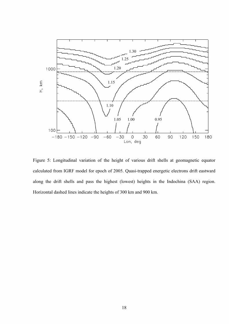
Because of asymmetrical orientation of the geomagnetic dipole, the height of top points

varies with longitude. Figure 5 shows longitudinal variation of the height of drift shells (L-

shells) calculated for the geomagnetic equator using IGRF model of epoch 2005.

Participating in a gradient drift, energetic electrons move eastward along the drift shells. One

can see that the L-shells are descending starting from the region of Indochina at longitudes of

~120°. In this region, the height of ~900 km corresponds to the L ~ 1.05. Above the Pacific

8

173

174

175

176

177

178

179

180

181

182

183

184

185

186

187

188

189

190

191

192

193

194

195

196

197

region, the altitude of top points for bouncing electron decreases with increasing longitude.

The drift shells rich minimal heights in the SAA region, where practically all the particles

quasi-trapped at L < 1.1 are lost. At altitudes of 1000 km and below, the period of the

azimuthal drift for 30 keV electrons is ~20 hours (Lyons and Williams, 1984). Hence, the

electrons with large pitch angles can make many thousands of bounces before they are lost in

the SAA region.

Taking into account the specific ionization of electrons (the energy loss per unit distance)

and standard vertical profile of the upper atmosphere (e.g. Dmitriev et al., 2008), we can

calculate the number of bounces between the top point at 800 km and mirror points at height

Hmin until the ~30 keV electron has lost whole of the energy in ionization. By this way, we

find that for Hmin below 600 km, the ~30 keV electrons lost whole energy within ~2 hours.

During this time, the electrons pass eastward no more than ~30° in longitudes, because of

very slow azimuthal drift. Hence, the quasi-trapped electrons, observed westward from the

longitude of -150°, have a quite high chance to lose whole of their energy in ionization of the

ionosphere. Because of arched magnetic field configuration, this ionization is released in the

region of geomagnetic latitudes above ~20°. It is important to note that the charged particle

spend most of time in vicinity of mirror point. Hence, the quasi-trapped electrons lose most

of energy rather at low to middle latitudes than at the equator. That corresponds well to the

spatial location of mid-latitude positive ionospheric storm.

Another important issue is conditions required for the downward transport of electrons from

the IRB to the heights below 1000 km. The well-know mechanism is a radial diffusion across

the drift shells. However, in the strong magnetic field at low altitudes this diffusion is very

slow that results in very weak fluxes of energetic electrons at the forbidden drift shells at low

latitudes. In contrast, geomagnetic storms are accompanied by a very strong penetrated

electric field of dawn-dusk direction. In the nightside, this electric field is pointed westward

9

that results in fast (a few hours) ExB drift of particles across the magnetic field lines toward

the Earth. Then the electrons drift eastward through morning sector toward noon.

198

199

200

201

202

203

204

205

206

207

208

209

210

We can summarize that during magnetic storm, the energetic electrons (~30 keV) drift fast

radially from the IRB to the ionospheric altitudes in the nightside sector. Drifting azimuthally

eastward, the quasi-trapped electrons loss the energy in ionization of the atmospheric gases

and, thus, produce abundant ionization of the mid-latitude ionosphere.

Acknowledgements

The authors thank a team of NOAA’s Polar Orbiting Environmental Satellites for providing

experimental data about energetic particles and Kyoto World Data Center for Geomagnetism

(http://wdc.kugi.kyoto-u.ac.jp/index.html) for providing the Dst, Kp and AE geomagnetic

indices. The Global Ionosphere Maps/VTEC Data from European Data Center was obtained

through ftp://ftp.unibe.ch/aiub/CODE/. The ACE solar wind data were provided by N. Ness

and D. J. McComas through the CDAWeb web site. We acknowledge Dr. Patrick Newell for

help with providing DMSP data. The DMSP particle detectors were designed by Dave Hardy

of AFRL, and data obtained from JHU/APL. This work was supported by grant NSC 99-

2811-M-008-093 and Ministry of Education under the Aim for Top University program at

NCU of Taiwan #985603-20.

211

212

213

214

215

216

217

218

219

220

221

222

References

Biktash, L., 2004. Role of the magnetospheric and ionospheric currents in generation of the

equatorial scintillations during geomagnetic storms. Annales Geophysicae 22, 3195-3202.

Balan, N., Shiokawa, K., Otsuka, Y., Kikuchi, T., Vijaya Lekshmi, D., Kawamura, S.,

Yamamoto, M., Bailey, G.J., 2010. A physical mechanism of positive ionospheric storms

10

223

224

225

226

227

228

229

230

231

232

233

234

235

236

237

238

239

240

241

242

243

244

245

246

at low latitudes and midlatitudes. J. Geophys. Res. 115, A02304.

doi:10.1029/2009JA014515.

Balan, N., Yamamoto, M., Liu, J.Y., Otsuka, Y., Liu, H., Luhr, H., 2011. New aspects of

thermospheric and ionospheric storms revealed by CHAMP. J. Geophys. Res. 116,

A07305. doi:10.1029/2010JA016399.

Dmitriev, A.V., Tsai, L.-C., H.-C. Yeh, Chang, C.-C., 2008. COSMIC/FORMOSAT-3

tomography of SEP ionization in the polar cap. Geophys. Res. Lett., 35, L22108.

doi:10.1029/2008GL036146.

Dmitriev, A.V., Jayachandran, P.T., Tsai, L.-C., 2010. Elliptical model of cutoff boundaries

for the solar energetic particles measured by POES satellites in December 2006. J.

Geophys. Res. 115, A12244. doi:10.1029/2010JA015380.

Evans, D.S., Greer, M.S., Polar Orbiting Environmental Satellite Space Environment

Monitor: 2. Instrument Descriptions and Archive Data Documentation, Tech. Memo.

version 1.4, NOAA Space Environ. Lab., Boulder, Colo., 2004.

Hajj, G.A., Lee, L.C., Pi, X., Romans, L.J., Schreiner, W.S., Straus, P.R., Wang, C., 2000.

COSMIC GPS ionospheric sensing and space weather. Terr. Atmos. Oceanic Sci. 11(1),

235-272.

Huston, S.L., Pfitzer, K.A., Space Environment Effects: Low-Altitude Trapped Radiation

Model, NASA/CR-1998-208593, Marshall Space Flight Center, Huntsville, AL, USA,

1998.

Lyons, L.R., Williams, D.J., 1984. Quantitative Aspects of Magnetospheric Physics, D.

Reidel Pub. Co., Dordrecht Boston.

Lei, J., Burns, A.G., Tsugawa, T., Wang, W., Solomon, S.C., Wiltberger, M., 2008.

Observations and simulations of quasiperiodic ionospheric oscillations and large-scale

11

247

248

249

250

251

252

253

254

255

256

257

258

259

260

261

262

263

264

265

266

traveling ionospheric disturbances during the December 2006 geomagnetic storm. J.

Geophys. Res. 113, A06310. doi:10.1029/2008JA013090.

Mendillo, M., 2006. Storms in the ionosphere: Patterns and processes for total electron

content. Rev. Geophys. 44, RG4001. doi:10.1029/ 2005RG000193 (2006).

Mendillo, M., Wroten, J., Roble, R., Rishbeth, H., 2010. The equatorial and low-latitude

ionosphere within the context of global modeling. J. Atmos. Sol. Terr. Phys. 72, 358-368.

doi:10.1016/j.jastp.2009.03.026.

Pedatella, N.M., Lei, J., Larson, K.M., Forbes, J.M., 2009. Observations of the ionospheric

response to the 15 December 2006 geomagnetic storm: Long-duration positive storm

effect. J. Geophys. Res. 114, A12313. doi:10.1029/2009JA014568.

Tsai, L.-C., Tsai, W.H., Chou, J.Y., Liu, C.H., 2006. Ionospheric tomography of the reference

GPS/MET experiment through the IRI model. Terr. Atmos. Oceanic Sci. 17, 263-276.

Tsurutani, B.T., et al., 2005. The October 28, 2003 extreme EUV solar flare and resultant

extreme ionospheric effects: Comparison to other Halloween events and the Bastille Day

event. Geophys. Res. Lett. 32, L03S09. doi:10.1029/2004GL021475.

Wei, Y., Hong, M., Pu, Z., et al., 2011. Responses of the ionospheric electric field to the

sheath region of ICME: A case study. J. Atmos. Sol. Terr. Physics 73, 123-129.

doi:10.1016/j.jastp.2010.03.004.

12

Figure 1: Global ionospheric maps of residual vertical total electron content (VTEC) between the

quiet day on December 3 and disturbed days on 15 December 2006 at 00-06 UT. Geomagnetic

equator is indicated by black curve. Local noon is depicted by vertical white dashed line. Strong

positive ionospheric storms are visible as large red spots.

13

14

Figure 2: COSMIC/FS3 3-D tomography of electron concentration (EC) at 04 - 06 UT on 15

December 2006: a) geographic map of residual total EC (TEC) obtained by subtraction of the

quiet-day TEC on December 3; b) meridional cut of EC in the range of longitudes from 130° to

135°. Geomagnetic equator is indicated by black curve. Local noon is depicted by vertical black

dashed line.

15

a

b Figure 3: Geographic distribution of >30 keV electron fluxes detected by a fleet of 5 POES

satellites at ~800 km altitude: (top panel) during magnetic quiet period on 2 - 4 December, 2006

and (bottom panel) during magnetic storm at 00 to 12 UT on 15 December 2006. Geomagnetic

equator is indicated by black curve.

16

0 1 2 3 4 5 6 7 8 9 10 11 12 13 14 15 16 17 18

Time, UT

1E+2

1E+3

1E+4

1E+5

1E+6

1E+7

Elec

tron

Flux

, (cm

2 s sr

)-1

0

20

40

60

80

100

dVTE

C, T

ECU

0

5

10

15Ey

, mV/

m

6

9

Kp

-200-150-100-50

0

Dst

, nT

1000

2000

AE, n

T

Figure 4: Variation of the interplanetary electric field Ey, geomagnetic indices, fluxes of >30 keV

magnetospheric electrons and ionospheric residual VTEC (dVTEC) during magnetic storm from

00 to 18 UT on 15 December (from top to bottom): Kp-index (gray) and Ey (black); Dst (black)

and AE (gray) indices; electron fluxes at ~120° longitude (red), at ~180° (violet), maximum

values of dVTEC at middle (black) and low (gray) latitudes.

17

1.30

1.25

1.20

1.15

1.10

1.05 1.00 0.95

Figure 5: Longitudinal variation of the height of various drift shells at geomagnetic equator

calculated from IGRF model for epoch of 2005. Quasi-trapped energetic electrons drift eastward

along the drift shells and pass the highest (lowest) heights in the Indochina (SAA) region.

Horizontal dashed lines indicate the heights of 300 km and 900 km.

18