lable at ScienceDirect

Atmospheric Environment 123 (2015) 129e138

Contents lists avai

Atmospheric Environment

journal homepage: www.elsevier .com/locate/atmosenv

On-road PM2.5 pollution exposure in multiple transportmicroenvironments in Delhi

Rahul Goel a, *, Shahzad Gani b, Sarath K. Guttikunda c, d, Daniel Wilson e, Geetam Tiwari a

a Transport Research and Injury Prevention Program, Indian Institute of Technology Delhi, New Delhi, 110016, Indiab Environmental and Water Resources Engineering, The University of Texas at Austin, TX, USAc Interdisciplinary Program in Climate Studies, Indian Institute of Technology Bombay, Mumbai, 400076, Indiad Division of Atmospheric Sciences, Desert Research Institute, Reno, NV, 89512, USAe University of California, Berkeley, USA

h i g h l i g h t s

� Measurements of on-road PM2.5 exposures in 11 transport microenvironments in Delhi.� Traveling in auto rickshaw leads to 30% higher exposure rate than in an off-road location.� Inside air-conditioned cars and metro carriages, the exposure rate is the lowest.� PM2.5 mass inhaled per km is 9 times for cycling compared to inside of an AC car.

a r t i c l e i n f o

Article history:Received 25 February 2015Received in revised form12 October 2015Accepted 12 October 2015Available online 20 October 2015

Keywords:PM2.5

Air pollutionRoad transportTrafficExposureDelhiIndia

* Corresponding author.E-mail address: rahulatiitd@gmail.com (R. Goel).

http://dx.doi.org/10.1016/j.atmosenv.2015.10.0371352-2310/© 2015 Elsevier Ltd. All rights reserved.

a b s t r a c t

PM2.5 pollution in Delhi averaged 150 mg/m3 from 2012 through 2014, which is 15 times higher than theWorld Health Organization's annual-average guideline. For this setting, we present on-road exposure ofPM2.5 concentrations for 11 transport microenvironments along a fixed 8.3-km arterial route, duringmorning rush hour. The data collection was carried out using a portable TSI DustTrak DRX 8433 aerosolmonitor, between January and May (2014). The monthly-average measured ambient concentrationsvaried from 130 mg/m3 to 250 mg/m3. The on-road PM2.5 concentrations exceeded the ambient mea-surements by an average of 40% for walking, 10% for cycle, 30% for motorised two wheeler (2W), 30% foropen-windowed (OW) car, 30% for auto rickshaw, 20% for air-conditioned as well as for OW bus, 20% forbus stop, and 30% for underground metro station. On the other hand, concentrations were lower by 50%inside air-conditioned (AC) car and 20% inside the metro rail carriage. We find that the percent ex-ceedance for open modes (cycle, auto rickshaw, 2W, OW car, and OW bus) reduces non-linearly withincreasing ambient concentration. The reduction is steeper at concentrations lower than 150 mg/m3 thanat higher concentrations. After accounting for air inhalation rate and speed of travel, PM2.5 mass uptakeper kilometer during cycling is 9 times of AC car, the mode with the lowest exposure. At current level ofconcentrations, an hour of cycling in Delhi during morning rush-hour period results in PM2.5 dose whichis 40% higher than an entire-day dose in cities like Tokyo, London, and New York, where ambient con-centrations range from 10 to 20 mg/m3.

© 2015 Elsevier Ltd. All rights reserved.

1. Introduction

Majority of the population in Indian subcontinent is exposed toambient particulate matter (PM) pollution levels much higher thanWorld Health Organization (WHO) guidelines (Dey et al., 2012).

According to Global Burden of Disease 2010 study, ambient PMpollution in India resulted in more than 600,000 deaths in 2010(Lim et al., 2013). According to a database of PM10 (PM with aero-dynamic diameter < 10 mm) pollution levels in more than 1600cities in the world in 2014, more than 40 cities from India areamong the 100 most polluted, with Delhi being the most pollutedof all (WHO, 2014). The annual average PM2.5 concentration for theperiod 2012 through 2014, reported by three air quality monitoringstations located across the city, was 150 mg/m3, which is

R. Goel et al. / Atmospheric Environment 123 (2015) 129e138130

approximately 4 times (hereafter indicated by �) higher than thenational ambient standard and 15� higher than the WHOguideline.

The direct links between emissions, outdoor air pollution, andhuman health have been extensively documented (IHME, 2013).Epidemiological studies have also linked PM2.5 as the robust indi-cator of adverse (mortality) impacts, and also the pollutant mostlinked to the vehicular exhaust emissions (Brauer et al., 2012). Thenegative health effects of traffic-related air pollution are also welldocumented (HEI, 2010). In on-road microenvironments, due tovicinity to tailpipe emissions, exposure to traffic-related PM ishigher than those in off-road locations (Kaur et al., 2007). Thetravel-related exposure to on-road PM pollution has been quanti-fied for different microenvironments, classified as travel modes,ventilation status (air conditioned or open windowed), type oftravel routes, and meteorological conditions. Table 1 summarizesmore than 20 studies in various settings from across the world,analyzing on-road exposure to PM2.5 pollution. The range of con-centrations in the table refers to the minimum and maximum re-ported average values among all the microenvironments (includingon-road modes and ambient location, and excluding undergroundrail). Apte et al. (2011) is the only study from India looking atexposure in three-wheeled auto rickshaws, and most studies arefrom cleaner high-income settings in the USA and the Europe. Theaverage ambient concentrations in these studies varied from 10 to70 mg/m3.

The cities in India differ significantly from the cities representedin Table 1. For instance, ambient PM2.5 concentrations in Indiancities are 4e8 times higher than most high-income settings (Deyet al., 2012; WHO, 2014), and vehicle ownership levels, expressedas number of vehicles per 1000 persons, are at least an order ofmagnitude lower (IMF, 2005; MoRTH, 2012). In case of Delhi, thismeans, a majority of trips are carried out using non-motorisedmodes, 2W, and bus-based public transportation (Pucher et al.,2007; RITES, 2010), leading to higher exposure rates compared tocities represented in Table 1, for the same amount of travel. How-ever, available literature has not adequately addressed the on-roadexposure of these modes in Indian cities.

In this paper, we present an approach to assess the on-roadexposure in various modes, analysis of the on-road exposure to

Table 1PM2.5 exposure studies for transport microenvironments (AR ¼ auto rickshaw).

Study Study year City

Rodes et al. (1999) 1997 Sacramento and Los Angeles (USA)Pfeifer et al. (1999) 1996 London (UK)Adams et al. (2001) 1999e2000 Central London (UK)Chan et al. (2002a) 1999e2000 Hong KongChan et al. (2002b) 2001 Guangzhou (China)Riediker et al. (2003) 2001 North Carolina (USA)Gomez-Perales et al. (2004) 2002 Mexico City (Mexico)Gulliver and Briggs (2004) 1999e2000 Northampton (UK)Chertok et al. (2004) 2002 Sydney (Australia)Kaur et al. (2005) 2003 Central London (UK)Aarnio et al. (2005) 2004 Helsinki (Finland)Fondelli et al. (2008) 2004 Florence (Italy)Fruin et al. (2008) 2003 Los Angeles (USA)McNabola et al. (2008) 2005e2006 Dublin (Ireland)Briggs et al. (2008) 2005 London (UK)Tsai et al. (2008) 2005 Taipei (Taiwan)Boogaard et al. (2009) 2006 Various cities (Netherlands)Morabia et al. (2009) 2007e2008 New York (USA)Zuurbier et al. (2010) 2007e2008 Arnhem (Netherlands)Apte et al. (2011) 2010 Delhi (India)de Nazelle et al. (2012) 2009 Barcelona (Spain)Quiros et al. (2013) 2011 California (USA)Weichenthal et al. (2015) 2010e2013 Montreal and Vancouver (Canada)

PM2.5 concentrations measured using optical PM monitor, and es-timates of inhaled doses of PM2.5 in 11 transport microenviron-ments e covering all motorised passenger-travel modes, walking,and cycling in Delhi.

2. Data and methods

2.1. PM2.5 pollution in Delhi

A summary of PM2.5 concentrations for years 2012 through2014, reported by three continuous air-quality monitoring stationse Punjabi Bagh, Mandir Marg, and R K Puram e operated by theDelhi Pollution Control Committee (DPCC), is presented in Fig. 1.The figure shows daily-average trend as well as month- and hour-specific averages for the three-year period. The locations of thethree stations are shown in Fig. 2. The particulate pollution in Delhihas a significant seasonal variation with highest concentrationsduring winter months from November through February (monthlyaverage rangee 200e250 mg/m3), and the lowest during monsoonmonths from July through September (70e100 mg/m3). The diurnaldistribution of pollution shows the highest concentrations duringlate night hours (10 PM through midnight) and early morning andrush-hour period (8 AM through 10 AM), and the lowest during theafternoon hours.

2.2. Study route

For measuring on-road exposure of PM2.5, we selected a routebetween Indian Institute of Technology Delhi campus (IIT), locatedin the southern part of the city at AurobindoMarg, and Union PublicService Commission office (UPSC), located at Shahjahan Road (seeFig. 2). The two end points for the study route were a bus stop infront of IIT located at the southbound approach of Aurobindo Marg,and the bus stop in front of UPSC at the southbound approach ofShahjahan Road. The total distance covered was 8.1 km; 5.6 kmwastraveled on Aurobindo Marg, 1.7 km on Prithviraj Road, and 0.8 kmon Shahjahan Road. Along the route, ward-level built-up density is~200 persons per hectare (pph), compared to Delhi's overall densityof 260 pph. Aurobindo Marg is one of the major arterial roads inDelhi running north-south, and caters to both inter-city as well as

Walk Cycle 2W Car AR Bus Train Tram PM2.5 (mg/m3)

* * 2e89* * 24e33

* * * * 13e39* * * 33e97

* * * 73e145* 22e24

* * 68e71* * 15e55

* 8e30* * * * 10e42

* 10e17* * 19e60* 8e110

* * * * 63e128* * 3e13

* * * * 22e68* * 6e122

* * * 13e24* * * 34e115

* * 110e170* * * * 21e35* * * 3e11

* 1e56

Fig. 1. (a) Daily and monthly average PM2.5 concentrations between January 2012 and December 2014 (b) Monthly variation in PM2.5 concentrations in 2012, 2013, and 2014 (c)Diurnal variation in PM2.5 concentrations in 2012, 2013, and 2014. For (b) and (c), the dot represents the mean; box plot represents 25th and 75th percentile, with median at thebreak; and whiskers represent the 5th and 95th.

Fig. 2. DPCC ambient air quality monitoring stations and on-road pollution exposure study route in Delhi.

R. Goel et al. / Atmospheric Environment 123 (2015) 129e138 131

intra-city traffic. The road connects Delhi with Gurgaon, the satel-lite city to the south of Delhi, and passes through highly denseresidential areas within southern part of Delhi. Thus the selectedroute is likely representative of the daily traffic conditions experi-enced by a traveler in Delhi region.

The average number of vehicles operating on Aurobindo Margfrom 8 AM to noon is 5100 per hour, with 52% cars, 27% 2W, 18%auto rickshaws, 2% buses and mini-buses, and less than 1% oflight commercial vehicles with no 2-axle or multi-axle trucks(CRRI, 2012). The absence of trucks in the vehicular mix is

R. Goel et al. / Atmospheric Environment 123 (2015) 129e138132

because heavy-duty diesel-based trucks are allowed to operatewithin the city only from 9 PM to 6 AM. On Prithviraj Road andShahjahan Road, no commercial goods vehicles are allowed asthey are located under the jurisdiction of New Delhi MunicipalCorporation (NDMC), which disallows the movement of com-mercial vehicles throughout the day. The first 4.1 km of the routenorth of IIT is heavily populated and has commercial land-usealong the roadside e mostly retail shops. The rest of the routenorthward lies within the jurisdiction of NDMC, is much lesspopulated, and has federal government offices and residentialsettlements for their staff members, with almost no commercialland-use along the route.

2.3. Data collection

Our data collection spanned from January through May 2014,and was carried out over 41 days during the five-month period. Foron-road travel, we recorded PM2.5 concentrations, along withrelative humidity (RH), geographical location, as well as speed oftravel. The study months were selected as they cover a wide rangeof PM2.5 concentrations, fromvery high in January to comparativelylower in May (see Fig. 1b). Also, this time of year has no rainfallwhich is required for the ease of data collection. Only a single in-strument was used for measuring PM2.5 concentrations, therefore,simultaneous measurements of ambient and in-vehicle concen-trations were not possible. Thus, ambient PM2.5 concentrationswere measured at the beginning and the end of the on-road trips.

We define a trip as a one-way journey between IIT and UPSC,regardless of the direction. The group of consecutive trips betweenthe two sets of ambient concentration measurements will bereferred to as a tour. We made a total of 75 tours, consisting of 150trips, from 8 AM to 1 PM, with 27 of those trips lasting past noon.The time period was selected to capture the rush hour trafficmovement. Among all the tours, 6 included more than 2 trips, andthe rest included 2 or fewer. We started most tours from IIT, inwhich case we measured ambient concentrations in a green spacein IIT campus at the beginning as well as at the end of the tour. For afew tours with only one trip, on one end, we measured ambientconcentrations at a house (second floor, balcony, height ~ 6 m) in aresidential locality within 3 km of UPSC (see AMB in Fig. 2), and onthe other end, at IIT. Except for 12 tours, we used only one mode oftravel. For 34 out of 75 tours, we measured ambient concentrationsonly in the beginning or in the end. We did not consider the tripsthat were discontinued in the middle due to long traffic jams, road-closures, or bus-route detours.

The measurements were made in a total of 11 different types ofmicroenvironments, covering all motorised passenger travel-modes operating in Delhi. This included 8 travel modes e cycle,2W, open-windowed car (OW car), air-conditioned car (AC car),auto rickshaw, open-windowed bus (OW bus), air-conditioned bus(AC bus), and metro. The air-conditioners of cars were set to recy-cled air mode. For metro, we traveled on the Yellow line from HauzKhas station (closest to IIT) to Udyog Bhawan station (closest toUPSC), which is the underground line parallel to study route. Themetro platforms, as well as the coaches, are air-conditioned. Out of~190 km of existing Delhi metro network, 48 km is underground,while the rest is elevated. The two stations are shown in Fig. 2.There are no bicycle lanes along the study route.

Rest of the 3 microenvironments are walk, and two types ofpublic transport (PT) stops e bus stops (close to IIT and UPSC), andmetro station. Unlike other modes, walking was carried out only fortraveling to bus stops and crossing the road. The measurements forbus stops and metro stations were carried out for the duration ofwaiting for bus and metro, respectively.

2.4. Instruments

We measured PM2.5 concentrations using a portable DustTrak(DT) DRX Aerosol Monitor (Model 8533, TSI Inc., USA), which em-ploys light scattering for real-time mass determination (TSI, 2012).The instrument has factory calibration of A1 Arizona ultrafine testdust (ISO 12103-1), at a relative humidity (RH) of 29%. Average RHvalues for the days of our data collection are e 62% (January), 45%(February), 45% (March), 36% (April), and 31% (May). Comparison ofRH and wind speed values to those of previous years show thatmeteorological conditions are representative of this time of year inDelhi (see Supplementary Material (SI)). In order to account for theerror in the measurement of the instrument due to RH, we used thecorrection reported by Ramachandran et al. (2003), also used byApte et al. (2011) for their PM2.5 exposure study in Delhi. The cor-rected PM2.5 reading is referred to as PM2.5RH-corrected. In addition,we calibrated the DT using gravimetric sampling, in which we co-located the gravimetric sampler (cyclone and filter) at IIT campusand a roadside location. The description of the calibration process isprovided in the SI. The calibration factor was generated to correctthe RH-corrected readings from DT. The RH-correction and thecalibration equation are shown in equations (1) and (2).

PM2:5RH�Corrected ¼ PM2:5DT1þ 0:25 RH2

1�RH

(1)

PM2:5 ¼ 1:34 ðPM2:5RH�CorrectedÞ0:93 (2)

To measure RH, we used a portable instrument (HOBO, ModelU10-003, Onset Computer Corporation, Massachusetts, USA). Forlogging time stamp, geographic location (latitude and longitude),and speed of movement, we used a GPS unit (Model AGL3080,AMOD Technology Company, Taipei, Taiwan). The GPS device isbased on SiRF-III technology and has a positional accuracy of 10 m.We used a frequency of 1 Hz for the three instruments and syn-chronized the data. The three instruments were carried by a volun-teer using a backpack. The DTwas kept in the backpackwith the inletof the conductive tube set at the breathing level of the volunteer.Further, the DT was padded inside the backpack to avoid suddenjerks during themovement of volunteer. The RH instrument and GPSunit were strapped to the outside of the backpack. All volunteerswho contributed to data collection for this study were non-smokers.

2.5. Data analysis

2.5.1. In-vehicle and ambient concentrationsOut of 75 tours, we measured ambient concentrations on both

ends of the tours for 41 tours, and for the rest, we measuredambient concentrations at either the beginning or the end of thetour. Note that a tour may have more than one microenvironment.For the cases when ambient concentrations were measured at bothends of a tour, we averaged the concentration readings at the twoends, and considered those as ambient concentrations corre-sponding to the on-road measurements. To give equal weightage tothe concentration readings for the two ends, we considered equalduration of measurement on both ends (average total duration ofmeasurements at the two ends ~7 min; average difference betweenthe two sets of measurements ~70 min). For the cases whenambient concentrations were measured only at the beginning or atthe end of the tours (n¼ 34), we used a correction factor to accountfor the missing concentration on one end (see SI).

2.6. Ratio of in-vehicle and ambient concentrations (Ƴ)

We calculated the ratio of average in-vehicle concentrations to

R. Goel et al. / Atmospheric Environment 123 (2015) 129e138 133

the average ambient concentrations, referred to as Y. Thus, Y-1indicates the fraction by which in-vehicle concentrations exceedsambient concentrations. For each mode, number of ratios calcu-lated is equal to the number of tours made using that mode. Table 2shows duration of measurement as well as overall average con-centration values for different microenvironments, classified bymonth, and Table 3 presents the number of tours and number ofone-way trips for each microenvironment.

2.6.1. Inhaled doseFor inter-modal comparisons, concentrations are not sufficient

to evaluate the full extent of the differences between the mass ofpollutants inhaled by different road-user types. This is becausepollution dose, i.e. the mass of pollutant inhaled, is also dependenton the minute ventilation rates (VR), which is a measure of amountof air inhaled per unit time, expressed in litres/minute. To estimateinhaled doses in various travel modes, we used distance-based andduration-based approaches. In the former, doses are estimated for agiven distance, which takes speed of travel in to account, and in thelatter, dose is estimated for a given duration of on-road travel. Forboth approaches, we estimated the dose for 5 km of travel, and forthe former, expressed it as per km and, for the latter, as per 15-min duration. For these estimates, we assumed an ambient con-centration of 165 mg/m3, which is the annual average concentrationfrom 8 AM through 12 noon. The average travel speed calculatedfrom GPS data and VR values for each microenvironment reportedby USEPA (2011) are presented in Table 3. For PT modes (bus andmetro), we also assumed 15-min out-of-vehicle movement ofpassengers e 10 min of walking for access and egress, and 5 min ofwaiting at bus stops and metro stations, respectively. The detailedequations for calculation of inhaled dose are provided in SI.

3. Results and discussion

3.1. Seasonal variation of ambient and in-vehicle concentrations

Our data collection includes winter (January), spring (Februar-yeMarch), and summer (AprileMay) seasons (see Table 2). The

Table 2Duration of measurement in minutes and PM2.5 concentrations (average, median, 5th perickshaw; MS ¼ metro station).

Month Location Ambient Walk Cycle 2W OW car

January Duration 79 35 139 e e

Average (SD) 253 (80) 231 (72) 347 (94) e e

Median 217 208 338 e e

p5 180 175 263 e e

p95 380 333 442 e e

February Duration 183 79 630 e e

Average (SD) 220 (121) 278 (223) 285 (141) e e

Median 211 248 270 e e

P5 66 104 129 e e

P95 425 491 509 e e

March Duration 65 53 e e e

Average (SD) 132 (71) 149 (102) e e e

Median 93 117 e e e

P5 50 59 e e e

P95 270 315 e e e

April Duration 209 82 e 529 385Average (SD) 157 (122) 234 (184) e 207 (139) 180 (105)Median 116 186 e 162 164P5 48 84 e 78 68P95 380 485 e 519 308

May Duration 18 4 e e e

Average (SD) 133 (51) 159 (122) e e e

Median 130 127 e e e

P5 73 101 e e e

P95 195 334 e e e

measured average (±standard deviation) ambient PM2.5 concen-tration during March through May (150 ± 109 mg/m3) was signifi-cantly lower than that in January and February (231 ± 113 mg/m3).The variation of PM2.5 concentrations over months can also beobserved for different on-road microenvironments. Average in-vehicle concentrations for AC bus vary from 315 mg/m3 in Januaryto 140 mg/m3 in April. Similar findings of seasonal variation of in-vehicle exposure of PM2.5 in Delhi were reported by Apte et al.(2011). The large variation over the months is due to the signifi-cant effect of meteorology on PM pollution in Delhi (Guttikundaand Gurjar, 2012). The seasonal variation is more significant insome modes than others. This is because not all modes werestudied simultaneously, and, even during summer months, somedays have ambient concentrations as high as during winters.

3.2. Ratio of in-vehicle and ambient concentrations (Y)

The average Y values along with their 95% confidence intervalsare shown in Fig. 3. AC car has the lowest average value of 0.5,followed by metro's 0.8, and for all other microenvironments,average values vary from 1.1 to 1.4. The ratios can be interpreted forinter modal comparisons. For instance, average ratios indicate thata 2W rider is exposed to 2.6� higher concentrations than a pas-senger in an AC car. We compared the average Y values estimatedfor cases in which ambient concentration measurements weredone on both ends of the tours with the cases with ambient con-centration only on one end (see SI). We found that the two sets ofestimates differ by 10e20%.

The value of Y estimated for open modes in this study (1.3) issimilar to the ratio (1.5) reported by Apte et al. (2011), also for Delhi,and to the ratio of near-road to off-road locations (1.1), in Bangalore(2011 populatione 8.5 million, located in southern part of India),reported by Both et al. (2011). Among the studies presented inTable 1, we reviewed studies which reported concentrations for on-road microenvironments as well as ambient location, and calcu-lated corresponding Y values. For cycling, Y varied from 1.5 to 3.4with an average of 2.0 (Adams et al., 2001; de Nazelle et al., 2012;Fondelli et al., 2008; McNabola et al., 2008; Zuurbier et al., 2010),

rcentile and 95th percentile) in mg/m3 for different microenvironments (AR ¼ auto

AC car AR OW bus AC bus Bus stop Metro MS

e 22 72 89 132 e e

e 255 (139) 295 (62) 315 (105) 248 (94) e e

e 240 284 319 205 e e

e 178 220 136 166 e e

e 328 399 470 383 e e

e 346 190 147 280 e e

e 241 (136) 293 (131) 278 (143) 301 (141) e e

e 236 280 247 319 e e

e 87 87 128 98 e e

e 430 492 517 482 e e

e 240 106 150 127 e e

e 159 (113) 187 (173) 132 (118) 176 (105) e e

e 137 160 102 158 e e

e 58 79 50 57 e e

e 318 350 284 311 e e

501 28 24 45 112 85 2756 (44) 257 (295) 277 (77) 140 (56) 195 (87) 87 (141) 141 (29)49 207 277 129 178 83 14118 96 207 88 89 56 97123 431 348 218 325 110 186e 39 e 27 32 66 43e 187 (330) e 113 (35) 120 (38) 76 (20) 142 (41)e 146 e 109 116 74 140e 85 e 84 94 60 73e 325 e 153 154 100 195

Table 3Summary of trips for different microenvironments.

Microenvironment Number of tours Number of one-way trips Average travel time for one-way trip (minutes) Speed (km/h) Minute ventilation (Litres/minute)

Cycle 12 24 28 17 352W 12 21 20 24 10OW Car 8 16 24 20 10AC Car 10 20 24 20 10Auto rickshaw 16 27 22 22 10OW Bus 12 15 28 14 10AC Bus 14 18 24 20 10Metro 5 9 14 32 10Walk 50 e e 4 15Bus stop 46 e e 10Metro station 6 e e 10

Fig. 3. Ratio of in-vehicle and ambient PM2.5 measurements during the on-road exposure study in multiple transport micro-environments in Delhi.

R. Goel et al. / Atmospheric Environment 123 (2015) 129e138134

and for cars, from 0.7 to 3.8 with an average of 2.1 (Adams et al.,2001; de Nazelle et al., 2012; McNabola et al., 2008; Riedikeret al., 2003; Zuurbier et al., 2010) in the cities of high-income Eu-ropean countries and the USA. In these settings, average ambientconcentrations varied from 10 to 70 mg/m3, compared to monthlyaverages of 130e250 mg/m3 over the period of our study. The valuesof Y estimated in our study (1.1 for cyclists and 0.5 for AC car) areclearly much lower. This indicates a higher correlation between in-vehicle and ambient concentrations in Delhi than in cleaner set-tings. However, even with lower difference between ambient andon-road concentrations, in-vehicle exposure in Delhi is an order ofmagnitude higher than those reported from the cleaner settings.

Higher values of Y in high-income countries with low pollutionlevels are likely because air in those settings may be pollutedlargely along the roads and much cleaner otherwise. This is incontrast with low-income countries, such as India, where share ofemissions from non-vehicular sources is also significant, resultingin high background concentrations. For instance, for a highly-trafficked location in Delhi, Pant et al. (2015) reported 16e19% ofPM2.5 concentrations attributed to primary vehicular exhaust. Onthe other hand, for major urban settings in France and the UK, shareof traffic-related sources to PM pollution has been reported to behigher than 40% (AIRPARIF, 2012; Lawrence et al., 2013). This isbecause, in high-income countries, industrial emissions havereduced as a result of stringent emission standards, domesticemissions as a result of universal use of gas-based fuels or elec-tricity, and diesel-generator emissions as a result of adequate po-wer availability. All these sources, on the other hand, continue to besignificant contributors to PM pollution in Indian cities (Guttikundaet al., 2014).

We found that the underground rail (metro) has 20% lowerPM2.5 concentrations than the ambient location. In contrast, studiesfrom London, Stockholm, and New York have reported up to 5� to20� higher PM2.5 concentrations in the underground rail than theoutside levels (Adams et al., 2001; Johansson and Johansson, 2003;Vilcassim et al., 2014). This difference between the concentrationsin metro systems is possible due to difference in the material of thewheels, ventilation levels, and breaking systems (Nieuwenhuijsenet al., 2007).

3.2.1. Relationship with ambient concentrationsFor the open modes, we calculated average Y classified by four

ranges of corresponding ambient concentrations e lower than 100,100e200, 200e300, and higher than 300 mg/m3. For this analysis,we excluded walk, as its exposure was not measured along theroute, unlike other modes. The average Y values for the four cate-gories are 1.6, 1.3, 1.1, and 1.0, respectively. A plot of Y values andambient concentrations is presented in Fig. 4, with a logarithmiccurve fitted over the data points (n ¼ 60). The ratios reduce non-linearly as the ambient concentrations increase, with steeperreduction at concentrations lower than 150 mg/m3 than at higherconcentrations. This trend is likely to arise if the concentrationscontributed by vehicles are largely constant and, as the backgroundconcentrations increase, the percent share of concentrationscontributed by vehicles reduces. This is also indicated by the sea-sonal differences in the source-apportionment of PM2.5 in Delhi. Forinstance, during winter months, concentrations increase due toadditional PM sources such as burning of wood and biomass forheating purposes, as well as operations of brick kilns and, as aresult, share of vehicular exhaust in overall PM pollution reduces

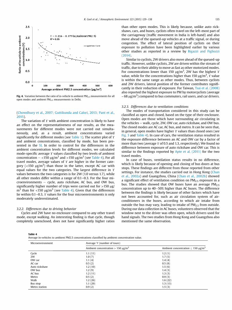
Fig. 4. Variation between the ratio of in-vehicle to ambient PM2.5 measurements for allopen modes and ambient PM2.5 measurements in Delhi.

R. Goel et al. / Atmospheric Environment 123 (2015) 129e138 135

(Chowdhury et al., 2007; Guttikunda and Calori, 2013; Pant et al.,2015).

The variation of Y with ambient concentration is likely to havean effect on the representativeness of our results, as the mea-surements for different modes were not carried out simulta-neously, and, as a result, ambient concentrations variedsignificantly for different modes (see Table 1). The scatter plot of Yand ambient concentrations, classified by mode, has been pre-sented in the SI. In order to control for the differences in theambient concentration levels for different modes, we calculatedmode-specific average Y values classified by two levels of ambientconcentration e <150 mg/m3 and >150 mg/m3 (see Table 4). For alltravel modes, average values of Y are higher in the former cate-gory (<150 mg/m3) than those in the latter, except AC car withequal values for the two categories. The largest difference in Y

values between the two categories is for 2W (1.0 versus 1.7), whileall other modes differ within a range of 0.1e0.3. For the four mi-croenvironments e cycle, auto rickshaw, AC bus, and OW bus,significantly higher number of trips were carried out for >150 mg/m3 than for <150 mg/m3 (see Table 4). Given that the differenceslie within 0.1e0.3, Y values for the four microenvironments is onlymoderately underestimated.

3.2.2. Differences due to driving behaviorCycles and 2W have no enclosure compared to any other travel

mode, except walking. An interesting finding is that cycle, thoughcompletely unenclosed, does not have significantly higher ratios

Table 4Average in-vehicles to ambient PM2.5 concentrations classified by ambient con

Microenvironment Average Ƴ (number of tours)

Ambient concentration > 150

Cycle 1.1 (11)2W 1.0 (7)OW car 1.1 (4)AC car 0.5 (2)Auto rickshaw 1.2 (10)OW bus 1.2 (9)AC bus 1.2 (11)Metro 0.5 (2)Walk 1.2 (26)Bus stop 1.1 (29)Metro station 0.9 (2)

than other open modes. This is likely because, unlike auto rick-shaws, cars, and buses, cyclists often travel on the left-most part ofthe carriageway (traffic movement in India is left-hand) and alsomove ahead of the queued-up vehicles at a traffic signal, or duringcongestion. The effect of lateral position of cyclists on theirexposure to pollution have been highlighted earlier by variousother studies as reported in a review by Bigazzi and Figliozzi(2014).

Similar to cyclists, 2Wdrivers alsomove ahead of the queued-uptraffic. However, unlike cyclists, 2W are drivenwithin the stream oftraffic, due to their ability tomove as fast as othermotorizedmodes.For concentrations lower than 150 mg/m3, 2W has the highest Y

value, while for the concentrations higher than 150 mg/m3, Y valueis within the same range as other modes. Thus, between cyclistsand 2W drivers, lateral position of the former contributes signifi-cantly in their reduction of exposure. For Taiwan, Tsai et al. (2008)also reported the highest exposure to PM by motorcyclists (average~ 68 mg/m3) compared to bus commuters, rail users, and car drivers.

3.2.3. Differences due to ventilation conditionsThe modes of transportation considered in this study can be

classified as open and closed, based on the type of their enclosure.Open modes are those which have surrounding air circulating inthe vehicles ewalk, cycle, 2W, OW car, auto rickshaw, and OW bus.The closed modes are AC car, AC bus, and metro. It can be seen that,in general, open modes have higher Y values than closed ones (seeFig. 3 and Table 4). In case of cars, the ventilation status resulted inthe exposure difference between an AC and OW car by a factor ofmore than two (average Y of 0.5 and 1.3, respectively). We found nodifference between exposure of auto rickshaw and OW car. This issimilar to the findings reported by Apte et al. (2011) for the twotravel modes.

In case of buses, ventilation status results in no difference,which is likely because of opening and closing of bus doors at busstops. These findings are different from those reported from othersettings. For instance, the studies carried out in Hong Kong (Chanet al., 2002a) and Guangzhou, China (Chan et al., 2002b) showeda significant effect of ventilation condition on PM2.5 exposure in abus. The studies showed that OW buses have an average PM2.5concentration up to 40e50% higher than AC buses. The differencebetween the findings is likely because of other factors which havenot been accounted for, such as air circulation system of air-conditioners in the buses, according to which air intake fromoutside the bus may vary, leading to intake of PM2.5 from outside.During our data collection in AC buses, volunteers observed that thewindow next to the driver was often open, which drivers used forhand signals. The two studies fromHong Kong and Guangzhou alsomentioned the same observation.

centration value.

mg/m3 Ambient concentration � 150 mg/m3

1.2 (1)1.7 (5)1.4 (4)0.5 (8)1.5 (6)1.4 (3)1.3 (3)0.9 (3)1.6 (22)1.3 (13)1.5 (3)

Fig. 6. Estimated annual PM2.5 emissions from on-road transport in Delhi (Goel andGuttikunda, 2015).

R. Goel et al. / Atmospheric Environment 123 (2015) 129e138136

3.3. Inhaled dose

Fig. 5 presents distance-based and duration-based inhaled doseof PM2.5. The dose estimates show higher inter-modal differencesfor distance-based estimates than duration-based, as the formeralso takes speed of travel into account, which varies over differentmodes. According to distance-based estimates, walk has the high-est dose per km, followed by cycle and bus, while AC car has thelowest, followed by metro. For buses, more than half of the totalintake dose is contributed from out-of-vehicle movement, while inthe case of metro, up to 80%. For a given distance, PM2.5 doseinhaled during cycling is 4� of 2W, 9� of AC car, and 4� of autorickshaw and, for a given duration, these ratios are 10�, 20� and9�, respectively. Active travel modes (walking and cycling) havelower travel speeds and their users have higher inhalation rates, ascompared to their non-active counterparts (2W, cars, auto rick-shaw, etc.) (see Table 3). This contributes to significantly higherinhaled dose for the active-mode users, even after controlling forthe exposed concentrations. For instance, evenwith similar value ofY, per-km inhaled dose of cycling will be 4� higher than an AC car.

4. Implications

For ambient concentration of 20 mg/m3 in the Netherlands, deHartog et al. (2010) estimated a dose of 35 mg for one hour ofcycling and 24-h dose of 274 mg. According to our estimates, just anhour of cycling in Delhi contributes to a dose of 393 mg (11� of 35 mgand 1.4� of 274 mg). Thus, with an annual average PM2.5 concen-tration of ~150 mg/m3, an individual in Delhi inhales more PM2.5

during less than an hour of cycling (representing two 30-min trips)than an individual inhales during the entire day in cities like Tokyo,Copenhagen (in Netherlands), London, New York, and Los Angeles,which have PM2.5 concentrations ranging from 10 to 20 mg/m3

(Hara et al., 2014; GLA, 2014; NYC, 2013). As another example, anindividual carrying out household cooking using biomass or coalburning is exposed to a concentration of 330 mg/m3 (Burnett et al.,2014) and, with an inhalation rate of 10 L per minute, inhales a doseof 200 mg in an hour. A cyclist in Delhi inhales twice that dose forthe same duration on the road.

The results of this study highlighted that the risk of travel-related pollution exposure, when expressed in terms of inhaleddose, is the lowest for cars and the highest for active modes oftransportation, followed by PT modes which also involve walkingfor a part of the trip. This implies socio-economic inequality oftravel-related pollution exposure, as those using cars in Delhi arelikely to have higher socio-economic status than those using non-motorised modes or PT. In 2011, only 20% of the households inDelhi owned a car (Census-India, 2012) and, in 2007, less than 10%of the total trips in Delhi were reported to be traveled by car (RITES,2010). The inequality of pollution exposure will be much less for

Fig. 5. Estimated inhaled dose of PM2.5 in multiple transport micro-environments inDelhi.

high-income countries, such as the USA and the UK, where 70% and90% of all the households, respectively, own at least one car(Giuliano and Dargay, 2006).

In the next 15 years, from 2015 through 2030, in-use fleet of 2Wis estimated to grow by 2.5� and that of cars by 3� and, in thebusiness-as-usual scenario, the particulate emissions are estimatedto increase by 1.5� (see Fig. 6). With an inevitable increase invehicle ownership, policies need to be formulated to control thegrowth of on-road emissions by setting higher emission standardsfor vehicles, and to curb the growing use of vehicles, throughbolstering of public transport services, higher parking charges, andmixed land-use development. If the current levels of pollutionlevels persist on road, individuals who can afford to, are likely toshift away from active modes as well as from PT. A comparativelylow value of Y indicates that on-road concentrations of PM2.5 arelargely contributed by non-vehicular sources. Thus, higher expo-sure of pollution during traveling in Indian cities should be seenwithin the broader framework of overall air pollution problem andnot from vehicular perspective alone, and the former is a result ofmultiple sectors in Indian cities other than road transport(Guttikunda et al., 2014). Therefore, policies aimed at reducingpollution from brick kilns, power plants, industries, and dieselgenerator sets are as important as policies for reducing vehicularpollution, for reducing travel-related hazard of air pollution.

5. Conclusions

We carried out measurements of in-vehicle exposure of PM2.5concentrations for 11 different transport microenvironments, on amajor arterial road in Delhi. Compared to all the studies presentedin Table 1 with a mix of low-, middle- and high-income settings, weobserved that on-road modes in Delhi experience the highestconcentrations. Among various travel modes, walking, cycling, anduse of PT result in the highest dose of particulate pollution, esti-mated for a unit of distance, or time, whereas traveling in an AC carleads to the least amount of dose. We find that, on an average,unenclosed travel modes in Delhi experience 10e40% higher PM2.5concentration than an ambient location. We reported a non-linearrelationship between Y and ambient concentration, and the latterhas a strong seasonal variation in Delhi (see Fig. 1). This implies thatthe relative difference between ambient and on-road concentrationis season dependent. This also underscores that, for settings such asDelhi, results of on-road exposure studies can differ considerablydepending on the season during which the study is conducted.

We estimated that the ratios of on-road to ambient concentra-tions are much lower in Delhi than those reported from settings inhigh-income countries with much cleaner air. However, even with

R. Goel et al. / Atmospheric Environment 123 (2015) 129e138 137

lower difference between in-vehicle and ambient concentrations,in-vehicle concentrations in Delhi are still an order of magnitudehigher than high-income settings due to high ambient/backgroundconcentration of the former. We attributed the reason for low ratiosto moderate contribution of traffic sources to PM2.5 pollution inDelhi, as reported by source-apportionment studies. PM pollutionin most Indian cities is a multi-sectoral problem, with transportcontributing a smaller fraction (Guttikunda et al., 2014) comparedto cleaner settings. Thus, in-vehicle to ambient concentration ratiosestimated in this study are equally likely to be applicable in othermajor Indian settings with high pollution levels. In addition, thelow values of ratio also indicate a higher correlation between on-road and background concentrations. Thus, ambient concentra-tion is a better surrogate of on-road exposure for open modes inIndian cities, than it is for cleaner high-income settings.

Acknowledgments

This work was partially supported by PURGE project (Publichealth impacts in URban environments of Greenhouse gas Emis-sions reductions strategies) funded by the European Commissionby its 7th Framework Programme under the Grant Agreement No.265325.

Appendix A. Supplementary data

Supplementary data related to this article can be found at http://dx.doi.org/10.1016/j.atmosenv.2015.10.037.

References

Aarnio, P., Yli-Tuomi, T., Kousa, A., M€akel€a, T., Hirsikko, A., H€ameri, K., ,et al.Jantunen, M., 2005. The concentrations and composition of and exposureto fine particles (PM2.5) in the Helsinki subway system. Atmos. Environ. 39 (28),5059e5066.

Adams, H.S., Nieuwenhuijsen, M.J., Colvile, R.N., 2001. Fine particle (PM2.5) personalexposure levels in transport microenvironments, London, UK. Sci. Total Environ.279 (1), 29e44.

AIRPARIF, 2012. Source Apportionment of Airborne Particles in the Ile-De-FranceRegion. Final Report. AIRPAIF, Paris, France.

Apte, Joshua S., Kirchstetter, Thomas W., Reich, Alexander H., Deshpande, Shyam J.,Kaushik, Geetanjali, Chel, Arvind, Marshall, Julian D., Nazaroff, WilliamW., 2011.Concentrations of fine, ultrafine, and black carbon particles in auto rickshaws inNew Delhi, India. Atmos. Environ. 45 (26), 4470e4480.

Bigazzi, A.Y., Figliozzi, M.A., 2014. Review of urban bicyclists' intake and uptake oftraffic-related air pollution. Transp. Rev. 34 (2), 221e245.

Boogaard, H., Borgman, F., Kamminga, J., Hoek, G., 2009. Exposure to ultrafine andfine particles and noise during cycling and driving in 11 Dutch cities. Atmos.Environ. 43 (27), 4234e4242.

Both, A.F., Balakrishnan, A., Joseph, B., Marshall, J.D., 2011. Spatiotemporal aspects ofreal-time PM2. 5: low-and middle-income neighborhoods in Bangalore, India.Environ. Sci. Technol. 45 (13), 5629e5636.

Brauer, M., Amann, M., Burnett, R.T., Cohen, A., Dentener, F., Ezzati, M., et al., 2012.Exposure assessment for estimation of the global burden of disease attributableto outdoor air pollution. Environ. Sci. Technol. 46 (2), 652e660.

Briggs, D.J., de Hoogh, K., Morris, C., Gulliver, J., 2008. Effects of travel mode onexposures to particulate air pollution. Environ. Int. 34 (1), 12e22.

Burnett, R.T., Pope, C.A., Ezzati, M., Olives, C., Lim, S.S., Mehta, S., Shin, H.H., et al.,2014. An integrated risk function for estimating the global burden of diseaseattributable to ambient fine particulate matter exposure. Environ. Health Per-spect. 122 (4), 397e403.

Census-India, 2012. Census of India, 2011. The Government of India, New Delhi,India.

Chan, L.Y., Lau, W.L., Lee, S.C., Chan, C.Y., 2002a. Commuter exposure to particulatematter in public transportation modes in Hong Kong. Atmos. Environ. 36 (21),3363e3373.

Chan, L.Y., Lau, W.L., Zou, S.C., Cao, Z.X., Lai, S.C., 2002b. Exposure level of carbonmonoxide and respirable suspended particulate in public transportation modeswhile commuting in urban area of Guangzhou, China. Atmos. Environ. 36 (38),5831e5840.

Chertok, M., Voukelatos, A., Sheppeard, V., Rissel, C., 2004. Comparison of airpollution exposure for five commuting modes in Sydney-car, train, bus, bicycleand walking. Health Promot. J. Aust. 15 (1), 63e67.

Chowdhury, Z., Zheng, M., Schauer, J.J., Sheesley, R.J., Salmon, L.G., Cass, G.R.,Russell, A.G., 2007. Speciation of ambient fine organic carbon particles and

source apportionment of PM2.5 in Indian cities. J. Geophys. Res. Atmos.(1984e2012) 112, D15.

CRRI, 2012. Personal Communications with Neelam Gupta. Central Road ResearchInstitute, Delhi.

de Hartog, J.J., Boogaard, H., Nijland, H., Hoek, G., 2010. Do the health benefits ofcycling outweigh the risks? Environ. Health Perspect. 1109e1116.

de Nazelle, A., Fruin, S., Westerdahl, D., Martinez, D., Ripoll, A., Kubesch, N.,Nieuwenhuijsen, M., 2012. A travel mode comparison of commuters' exposuresto air pollutants in Barcelona. Atmos. Environ. 59, 151e159.

Dey, S., Di Girolamo, L., van Donkelaar, A., Tripathi, S.N., Gupta, T., Mohan, M., 2012.Variability of outdoor fine particulate (PM2.5) concentration in the Indiansubcontinent: a remote sensing approach. Remote Sens. Environ. 127, 153e161.

Fondelli, M.C., Chellini, E., Yli-Tuomi, T., Cenni, I., Gasparrini, A., Nava, S., ,et al.Jantunen, M., 2008. Fine particle concentrations in buses and taxis inFlorence, Italy. Atmos. Environ. 42 (35), 8185e8193.

Fruin, S., Westerdahl, D., Sax, T., Sioutas, C., Fine, P.M., 2008. Measurements andpredictors of on-road ultrafine particle concentrations and associated pollut-ants in Los Angeles. Atmos. Environ. 42 (2), 207e219.

GLA, 2014. Average Air Quality Levels, Greater London Authority [computer file],accessed from. https://www.london.gov.uk/priorities/environment/consultations/air-quality.

Goel, R., Guttikunda, S.K., 2015. Evolution of On-Road Vehicle Exhaust Emissions inDelhi. Atmospheric Environment.

Gomez-Perales, J.E., Colvile, R.N., Nieuwenhuijsen, M.J., Fernandez-Bremauntz, A.,Gutierrez-Avedoy, V.J., Paramo-Figueroa, V.H., , et al.Ortiz-Segovia, E., 2004.Commuters' exposure to PM2.5, CO, and benzene in public transport in themetropolitan area of Mexico City. Atmos. Environ. 38 (8), 1219e1229.

Giuliano, G., Dargay, J., 2006. Car ownership, travel and land use: a comparison ofthe US and Great Britain. Transp. Res. Part A Policy Pract. 40 (2), 106e124.

Gulliver, J., Briggs, D.J., 2004. Personal exposure to particulate air pollution intransport microenvironments. Atmos. Environ. 38 (1), 1e8.

Guttikunda, S.K., Gurjar, B.R., 2012. Role of meteorology in seasonality of airpollution in megacity Delhi, India. Environ. Monit. Assess. 184 (5), 3199e3211.

Guttikunda, S.K., Calori, G., 2013. A GIS based emissions inventory at 1 km � 1 kmspatial resolution for air pollution analysis in Delhi, India. Atmos. Environ. 67,101e111.

Guttikunda, S.K., Goel, R., Pant, P., 2014. Nature of air pollution, emission sources,and management in the Indian cities. Atmos. Environ. 95, 501e510.

Hara, K., et al., 2014. Difference in concentration trends of airborne particulatematter during rush hour on weekdays and sundays in Tokyo, Japan. J. Air WasteManag. Assoc. 64 (9), 1045e1053.

Health Effects Institute (HEI), 2010. Traffic-related Air Pollution: a Critical Review ofthe Literature on Emissions, Exposure, and Health Effects (Special Report 17).Health Effects Institute, Boston, MA.

IHME, 2013. GBD Arrow Diagram. Institute for Health Metrics and Evaluation,University of Washington, Seattle, WA. Available from: http://vizhub.healthdata.org/irank/arrow.php (accessed 10.11.14.).

IMF, 2005. Will the oil continue to be tight?. In: World Economic Outlook, Globaland External Imbalances. International Monetary Fund, Washington D.C., US,pp. 157e183.

Johansson, C., Johansson, P.-Å., 2003. Particulate matter in the underground ofStockholm. Atmos. Environ. 37 (1), 3e9.

Kaur, S., Nieuwenhuijsen, M.J., Colvile, R.N., 2007. Fine particulate matter and car-bon monoxide exposure concentrations in urban street transport microenvi-ronments. Atmos. Environ. 41 (23), 4781e4810.

Kaur, S., Nieuwenhuijsen, M., Colvile, R., 2005. Personal exposure of street canyonintersection users to PM2.5, ultrafine particle counts and carbon monoxide inCentral London, UK. Atmos. Environ. 39 (20), 3629e3641.

Lawrence, S., Sokhi, R., Ravindra, K., Mao, H., Prain, H.D., Bull, I.D., 2013. Sourceapportionment of traffic emissions of particulate matter using tunnel mea-surements. Atmos. Environ. 77, 548e557.

Lim, S.S., Vos, T., Flaxman, A.D., Danaei, G., Shibuya, K., Adair-Rohani, H., ,et al.Davis, A., 2013. A comparative risk assessment of burden of disease andinjury attributable to 67 risk factors and risk factor clusters in 21 regions,1990e2010: a systematic analysis for the Global Burden of Disease Study 2010.Lancet 380 (9859), 2224e2260.

McNabola, A., Broderick, B.M., Gill, L.W., 2008. Relative exposure to fine particulatematter and VOCs between transport microenvironments in Dublin: personalexposure and uptake. Atmos. Environ. 42 (26), 6496e6512.

Morabia, A., Amstislavski, P.N., Mirer, F.E., Amstislavski, T.M., Eisl, H., Wolff, M.S.,Markowitz, S.B., 2009. Air pollution and activity during transportation by car,subway, and walking. Am. J. Prev. Med. 37 (1), 72e77.

MoRTH, 2012. Road Transport Year Book (2011-12). Transport Research Wing,Ministry of Road Transport and Highways, Government of India, New Delhi.

Nieuwenhuijsen, M., et al., 2007. Levels of particulate air pollution, its elementalcomposition, determinants and health effects in metro systems. Atmos. Envi-ron. 41 (37), 7995e8006.

NYC, 2013. New York City Trends in Air Quality Pollution and its Health Conse-quences. NYC Health, City of New York, USA.

Pant, P., Shukla, A., Kohl, S.D., Chow, J.C., Watson, J.G., Harrison, R.M., 2015. Char-acterization of ambient PM2.5 at a pollution hotspot in New Delhi, India andinference of sources. Atmos. Environ. 109, 178e189.

Pfeifer, G.D., Harrison, R.M., Lynam, D.R., 1999. Personal exposures to airbornemetals in London taxi drivers and office workers in 1995 and 1996. Sci. TotalEnviron. 235 (1), 253e260.

R. Goel et al. / Atmospheric Environment 123 (2015) 129e138138

Pucher, J., Peng, Z.R., Mittal, N., Zhu, Y., Korattyswaroopam, N., 2007. Urban trans-port trends and policies in China and India: impacts of rapid economic growth.Transp. Rev. 27 (4), 379e410.

Quiros, D.C., Lee, E.S., Wang, R., Zhu, Y., 2013. Ultrafine particle exposures whilewalking, cycling, and driving along an urban residential roadway. Atmos. En-viron. 73, 185e194.

Ramachandran, G., Adgate, J.L., Pratt, G.C., Sexton, K., 2003. Characterizing indoorand outdoor 15 minute average PM2.5 concentrations in urban neighborhoods.Aerosol Sci. Technol. 37 (1), 33e45.

Riediker, M., Williams, R., Devlin, R., Griggs, T., Bromberg, P., 2003. Exposure toparticulate matter, volatile organic compounds, and other air pollutants insidepatrol cars. Environ. Sci. Technol. 37 (10), 2084e2093.

RITES, 2010. Transport Demand Forecast Study and Development of an IntegratedRoad Cum Multi-modal Public Transport Network for NCT of Delhi. HouseholdInterview Survey Report, Chapter-4, Travel Characteristics. RITES Ltd.

Rodes, C., Sheldon, L., Whitaker, D., Clayton, A., Fitzgerald, K., 1999. MeasuringConcentrations of Selected Air Pollutants inside California Vehicles. Final Report(No. PBe99e161028/XAB). Research Triangle Inst., Research Triangle Park, NC(US). Sierra Research, Inc., Sacramento, CA (US); Aerosol Dynamics, Inc., Ber-keley, CA (US); Nevada Univ. System, Reno, NV (US); California State Air Re-sources Board, Sacramento, CA (US); Research Triangle Inst., Durham, NC (US).

Tsai, D.H., Wu, Y.H., Chan, C.C., 2008. Comparisons of commuter's exposure to

particulate matters while using different transportation modes. Sci. Total En-viron. 405 (1), 71e77.

TSI, 2012. DUSTTRAK DRX Aerosol Monitor- Theory of Operation. TSI Incorporated,USA.

U.S. Environmental Protection Agency (USEPA), 2011. Exposure Factors Handbook,2011 Edition. National Center for Environmental Assessment, Washington, DC.EPA/600/R-09/052F. Available from: the National Technical Information Service,Springfield, VA, and online at. http://www.epa.gov/ncea/efh.

Vilcassim, M.R., Thurston, G.D., Peltier, R.E., Gordon, T., 2014. Black carbon andparticulate matter (PM2.5) concentrations in New York City's subway stations.Environ. Sci. Technol. 48 (24), 14738e14745.

Weichenthal, S., Van Ryswyk, K., Kulka, R., Sun, L., Wallace, L.A., Joseph, L., 2015. In-vehicle exposures to particulate air pollution in Canadian metropolitan areas:the Urban Transportation Exposure Study. Environmental Science &Technology.

WHO, 2014. Outdoor Air Pollution in the World Cities. World Health Organization,Geneva, Switzerland.

Zuurbier, M., Hoek, G., Oldenwening, M., Lenters, V.C., Meliefste, K., Hazel, P.,Brunekreef, B., 2010. Commuters' exposure to particulate matter air pollution isaffected by mode of transport, fuel type, and route. Environ. Health Perspect.118 (6), 783e789.