On Scheduling Mechanisms: Theory, Practice and Pricing

Ahuva Mu’alemSISL, Caltech

Motivation

• Mechanisms ≈ auctions & reverse-auctions ≈ optimization problemswith strategic constraints

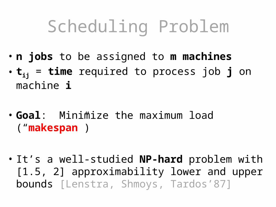
Scheduling Problem

• n jobs to be assigned to m machines• tij = time required to process job j on machine i

• Goal: Minimize the maximum load (“makespan”)

• It’s a well-studied NP-hard problem with [1.5, 2] approximability lower and upper bounds [Lenstra, Shmoys, Tardos’87]

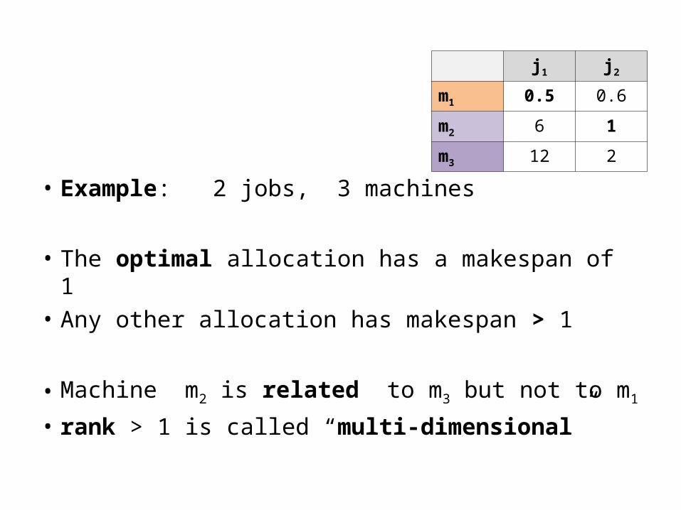
• Example: 2 jobs, 3 machines

• The optimal allocation has a makespan of 1• Any other allocation has makespan > 1

• Machine m2 is related to m3 but not to m1

• rank > 1 is called “multi-dimensional”

j1 j2

m1 0.5 0.6

m2 6 1

m3 12 2

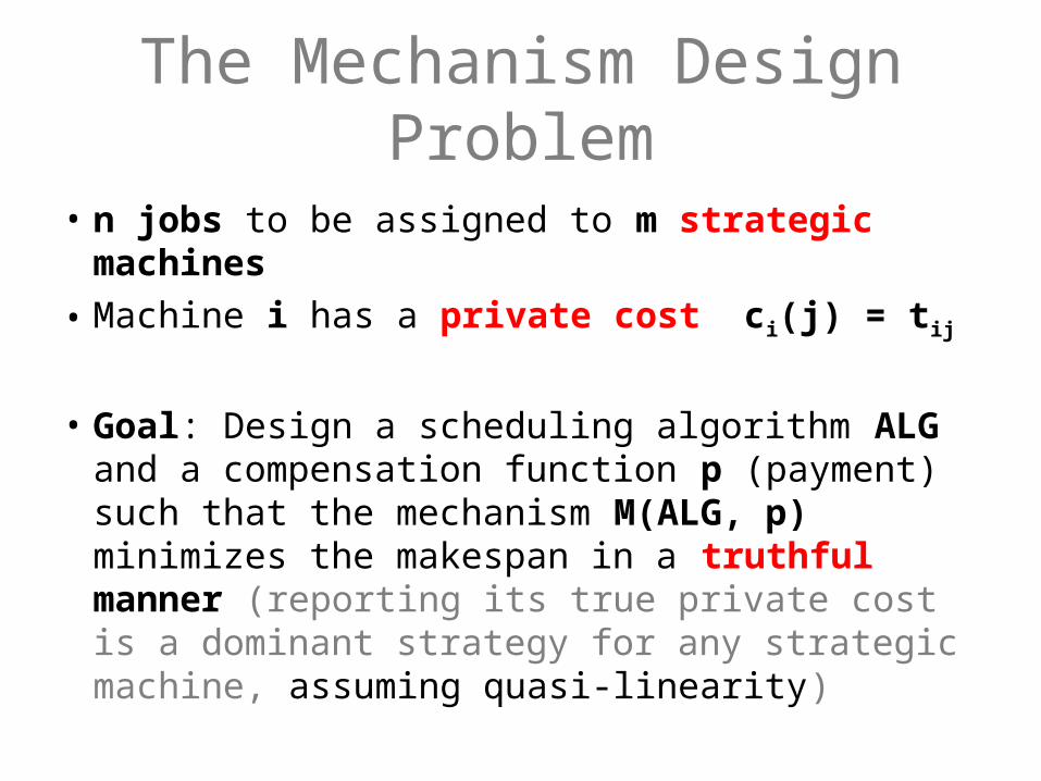
The Mechanism Design Problem

• n jobs to be assigned to m strategic machines• Machine i has a private cost ci(j) = tij

• Goal: Design a scheduling algorithm ALG and a compensation function p (payment) such that the mechanism M(ALG, p) minimizes the makespan in a truthful manner (reporting its true private cost is a dominant strategy for any strategic machine, assuming quasi-linearity)

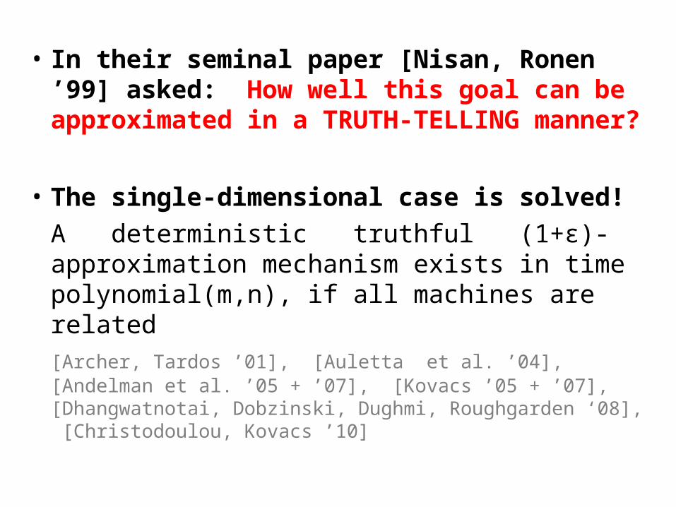
• In their seminal paper [Nisan, Ronen ’99] asked: How well this goal can be approximated in a TRUTH-TELLING manner?

• The single-dimensional case is solved!A deterministic truthful (1+ε)-approximation mechanism exists in time polynomial(m,n), if all machines are related [Archer, Tardos ’01], [Auletta et al. ’04], [Andelman et al. ’05 + ’07], [Kovacs ’05 + ’07], [Dhangwatnotai, Dobzinski, Dughmi, Roughgarden ‘08], [Christodoulou, Kovacs ’10]

The Multi-Dimensional Case

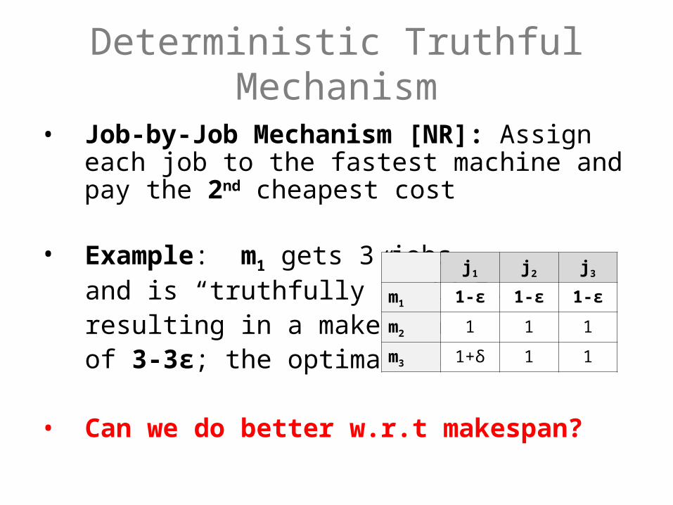
Deterministic Truthful Mechanism

• Example: m1 gets 3 jobs, and is “truthfully” paid 3, resulting in a makespan of 3-3ε; the optimal is 1

• Can we do better w.r.t makespan?

• Job-by-Job Mechanism [NR]: Assign each job to the fastest machine and pay the 2nd cheapest cost

j1 j2 j3

m1 1-ε 1-ε 1-ε

m2 1 1 1

m3 1+δ 1 1

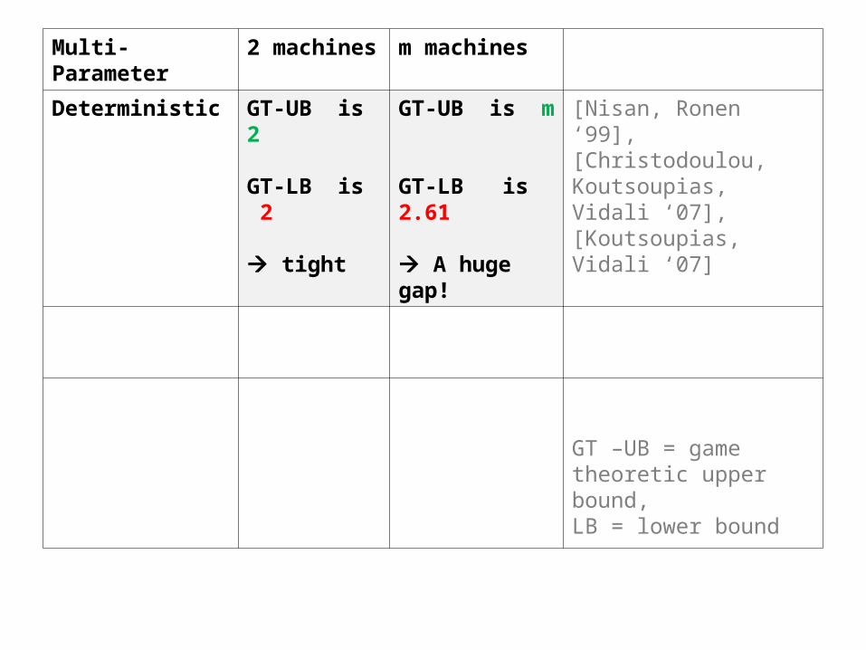
Multi-Parameter 2 machines m machines

Deterministic GT-UB is 2

GT-LB is 2

tight

GT-UB is m

GT-LB is 2.61

A huge gap!

[Nisan, Ronen ‘99], [Christodoulou, Koutsoupias, Vidali ‘07], [Koutsoupias, Vidali ‘07]

GT –UB = game theoretic upper bound, LB = lower bound

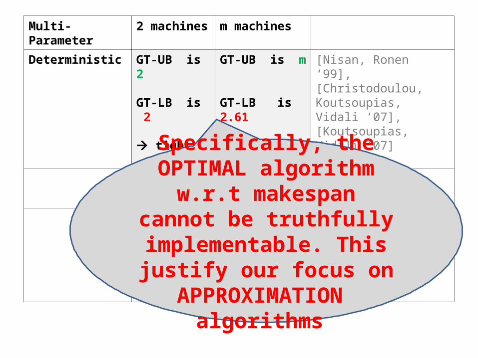
Multi-Parameter 2 machines m machines

Deterministic GT-UB is 2

GT-LB is 2

tight

GT-UB is m

GT-LB is 2.61

A huge gap!

[Nisan, Ronen ‘99], [Christodoulou, Koutsoupias, Vidali ‘07], [Koutsoupias, Vidali ‘07]

Specifically, the OPTIMAL algorithm w.r.t makespan

cannot be truthfully implementable. This justify

our focus on APPROXIMATION algorithms

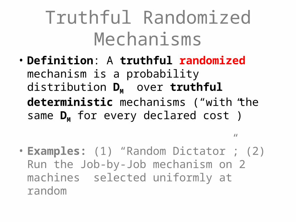
Truthful Randomized Mechanisms

• Definition: A truthful randomized mechanism is a probability distribution DM over truthful deterministic mechanisms (“with the same DM for every declared cost”)

• Examples: (1) “Random Dictator”; (2) Run the Job-by-Job mechanism on 2 machines selected uniformly at random

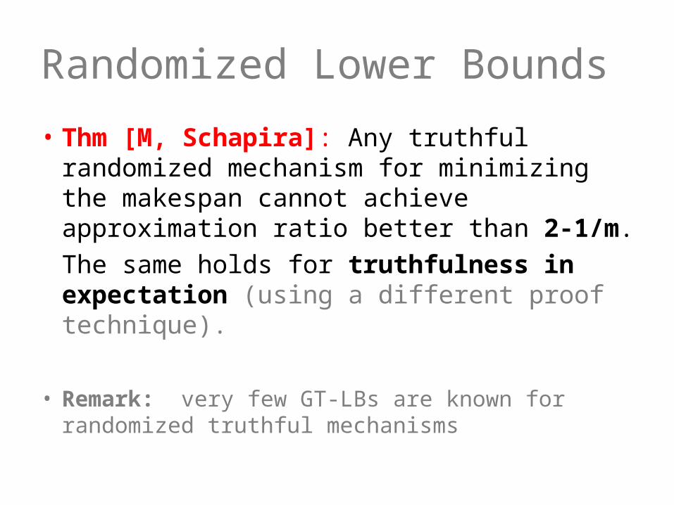
Randomized Lower Bounds

• Thm [M, Schapira]: Any truthful randomized mechanism for minimizing the makespan cannot achieve approximation ratio better than 2-1/m. The same holds for truthfulness in expectation (using a different proof technique).

• Remark: very few GT-LBs are known for randomized truthful mechanisms

Proof Idea

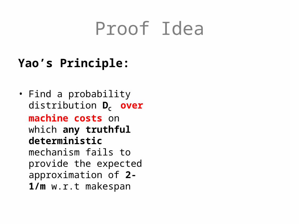
Yao’s Principle:

• Find a probability distribution DC over machine costs on which any truthful deterministic mechanism fails to provide the expected approximation of 2-1/m w.r.t makespan

Weak-Monotonicity:

• Theorem [BCRMNS ‘06]: If M(ALG, p) is a truthful mechanism then for every costs ci, di, c-i it holds that

ci(Si) + di(Ti) ≤ di(Si) + ci (Ti)

where ALG(ci, c-i) = Si and ALG(di, c-i) = Ti

Proof Idea

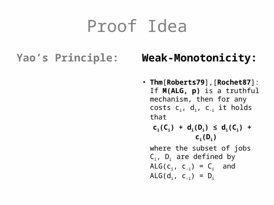
Yao’s Principle:

• Find a probability distribution over inputs on which any truthful deterministic mechanism fails to provide the expected approximation ratio of 2-1/m w.r.t makespan

Weak-Monotonicity:

• Thm[Roberts79],[Rochet87]: If M(ALG, p) is a truthful mechanism, then for any costs ci, di, c-i it holds that

ci(Ci) + di(Di) ≤ di(Ci) + ci(Di)

where the subset of jobs Ci, Di are defined by ALG(ci, c-i) = Ci and ALG(di, c-i) = Di

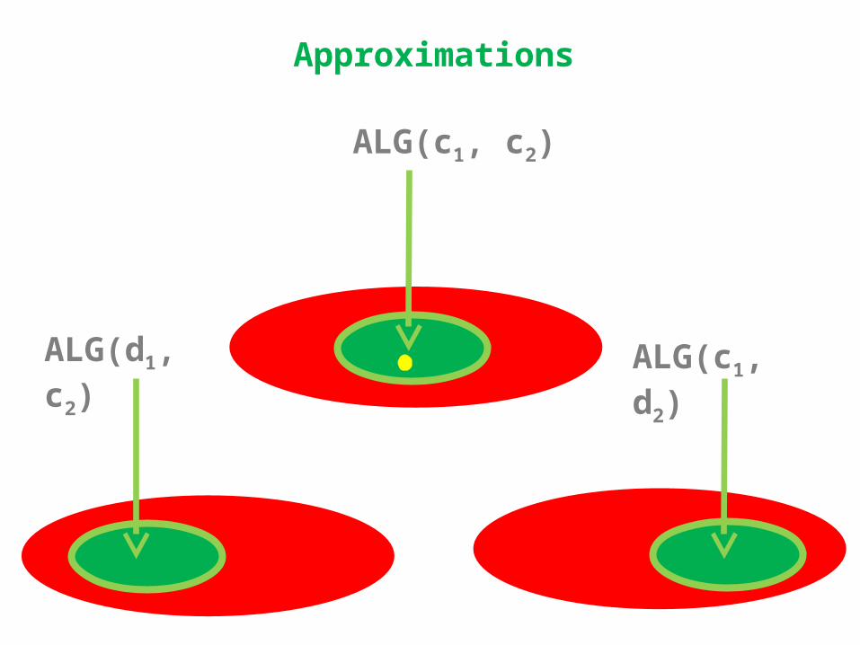
ALG(c1, c2)

Approximations

ALG(d1, c2) ALG(c1, d2)

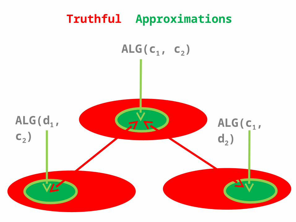
ALG(c1, c2)

Truthful Approximations

ALG(d1, c2) ALG(c1, d2)

j1 j2 j3

m1 4 99/ε 4

m2

99/ε 4 4

Randomized Lower Bound

j1 j2 j3

m1 4 99/ε 4

m2

99/ε ε 4+ε

j1 j2 j3

m1 ε 99/ε 4+ε

m2

99/ε 4 4

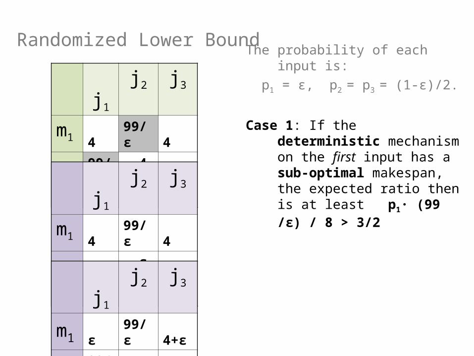
The probability of each input is:

p1 = ε, p2 = p3 = (1-ε)/2.

Case 1: If the deterministic mechanism on the first input has a sub-optimal makespan the expected ratio then is at least p1·(99 /ε)/8 > 3/2

Case 2: Otherwise, suppose wlog it allocates j1 to m1, and j2, j3 to m2, the best it can do on the third input is a makepan of 8 (without violation of weak-monotonicity), the expected ratio then is at least:

p2 · 8 / (4+2ε) + p3 · 1 = 3/2 - ε’

j1 j2 j3

m1 4 99/ε 4

m2

99/ε 4 4

Randomized Lower Bound

j1 j2 j3

m1 4 99/ε 4

m2

99/ε ε 4+ε

j1 j2 j3

m1 ε 99/ε 4+ε

m2

99/ε 4 4

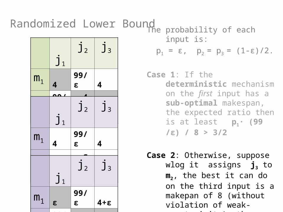
The probability of each input is:

p1 = ε, p2 = p3 = (1-ε)/2.

Case 1: If the deterministic mechanism on the first input has a sub-optimal makespan, the expected ratio then is at least p1· (99 /ε) / 8 > 3/2

Case 2: Otherwise, suppose wlog it allocates j3 to m2, the best it can do on the third input is a makepan of 8 (without violation of weak-monotonicity), the expected ratio then is at least:

p2 · 8 / (4+2ε) + p3 · 1 = 3/2 - ε’

j1 j2 j3

m1 4 99/ε 4

m2

99/ε 4 4

Randomized Lower Bound

j1 j2 j3

m1 4 99/ε 4

m2

99/ε ε 4+ε

j1 j2 j3

m1 ε 99/ε 4+ε

m2

99/ε 4 4

The probability of each input is:

p1 = ε, p2 = p3 = (1-ε)/2.

Case 1: If the deterministic mechanism on the first input has a sub-optimal makespan, the expected ratio then is at least p1· (99 /ε) / 8 > 3/2

Case 2: Otherwise, suppose wlog it assigns j3 to m2, the best it can do on the third input is a makepan of 8 (without violation of weak-monotonicity), the expected ratio then is at least:

p2 · 8 / (4+2ε) + p3 · 1 = 3/2 - ε’

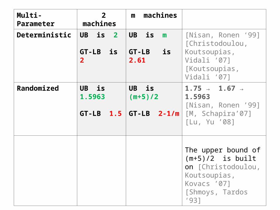
Multi-Parameter 2 machines m machines

Deterministic UB is 2

GT-LB is 2

UB is m

GT-LB is 2.61

[Nisan, Ronen ‘99] [Christodoulou, Koutsoupias, Vidali ‘07] [Koutsoupias, Vidali ‘07]

Randomized UB is 1.5963

GT-LB 1.5

UB is (m+5)/2

GT-LB 2-1/m

1.75 → 1.67 → 1.5963[Nisan, Ronen ’99][M, Schapira’07][Lu, Yu ’08]

The upper bound of (m+5)/2 is built on [Christodoulou, Koutsoupias, Kovacs ’07] [Shmoys, Tardos ‘93]

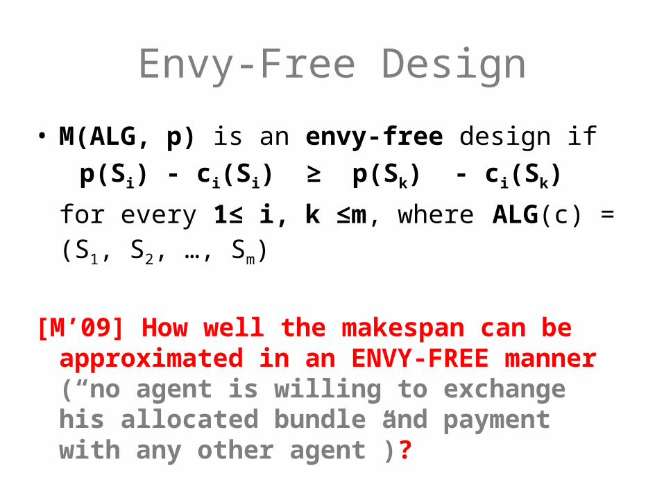
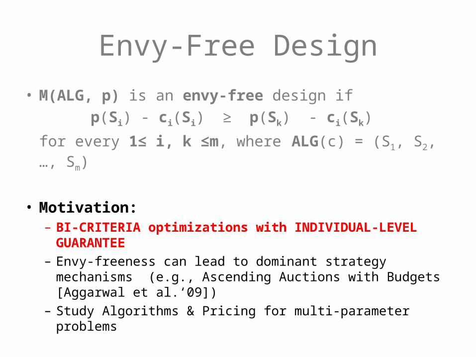
Envy-Free Design

• M(ALG, p) is an envy-free design ifp(Si) - ci(Si) ≥ p(Sk) - ci(Sk)

for every 1≤ i, k ≤m, where ALG(c) = (S1, S2, …, Sm)

[M’09] How well the makespan can be approximated in an ENVY-FREE manner (“no agent is willing to exchange his allocated bundle and payment with any other agent”)?

Envy-Free Design

• M(ALG, p) is an envy-free design ifp(Si) - ci(Si) ≥ p(Sk) - ci(Sk)

for every 1≤ i, k ≤m, where ALG(c) = (S1, S2, …, Sm)

• Motivation:– BI-CRITERIA optimizations with INDIVIDUAL-LEVEL

GUARANTEE – Envy-freeness can lead to dominant strategy mechanisms

(e.g., Ascending Auctions with Budgets [Aggarwal et al.‘09])– Study Algorithms & Pricing for multi-parameter problems

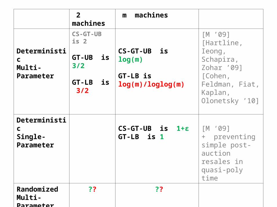
2 machines m machines

Deterministic Multi-Parameter

CS-GT-UB is 2

GT-UB is 3/2

GT-LB is 3/2

CS-GT-UB is log(m)

GT-LB is log(m)/loglog(m)

[M ’09] [Hartline, Ieong, Schapira, Zohar ’09] [Cohen, Feldman, Fiat, Kaplan, Olonetsky ’10]

DeterministicSingle-Parameter CS-GT-UB is 1+ε

GT-LB is 1

[M ‘09]+ preventing simple post-auction resales in quasi-poly time

RandomizedMulti-Parameter

?? ??

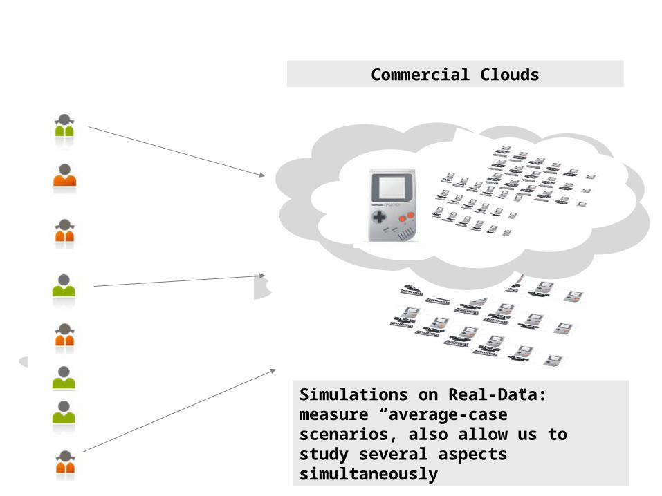
Commercial Clouds

Simulations on Real-Data: measure “average-case” scenarios, also allow us to study several aspects simultaneously

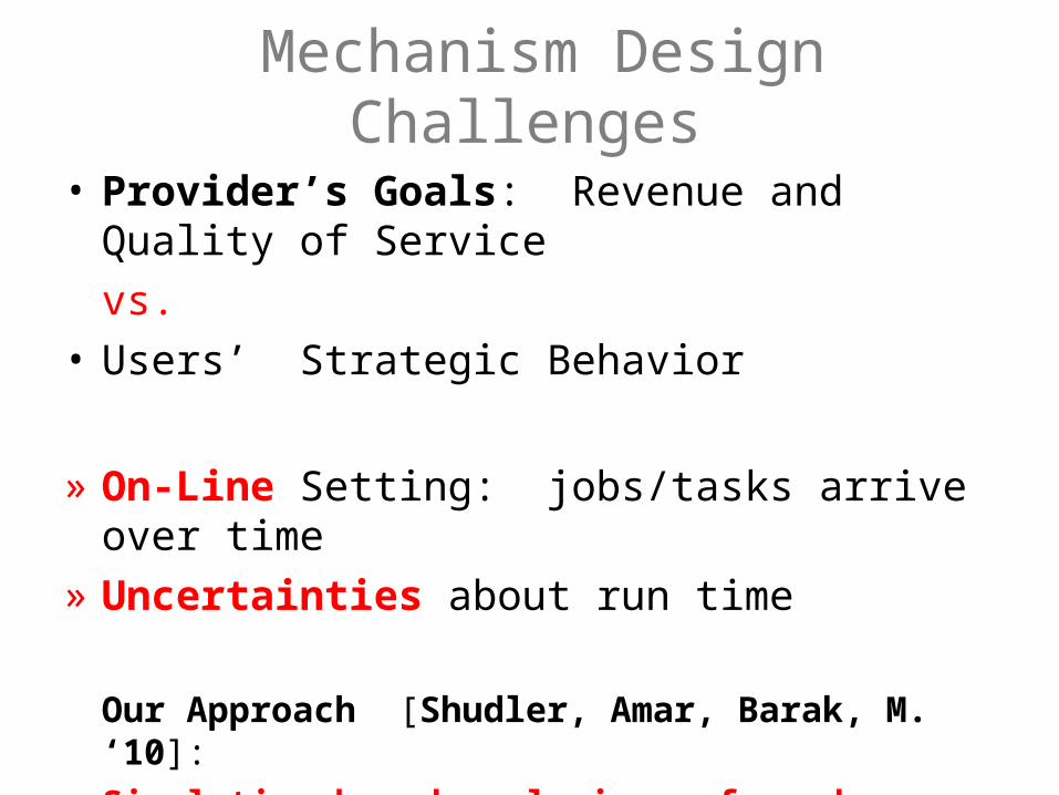
Mechanism Design Challenges

• Provider’s Goals: Revenue and Quality of Service

vs. • Users’ Strategic Behavior

» On-Line Setting: jobs/tasks arrive over time» Uncertainties about run time

Our Approach [Shudler, Amar, Barak, M. ‘10]:

Simulation-based analysis performed on real data taken from The Parallel Workload Archive @HUJI

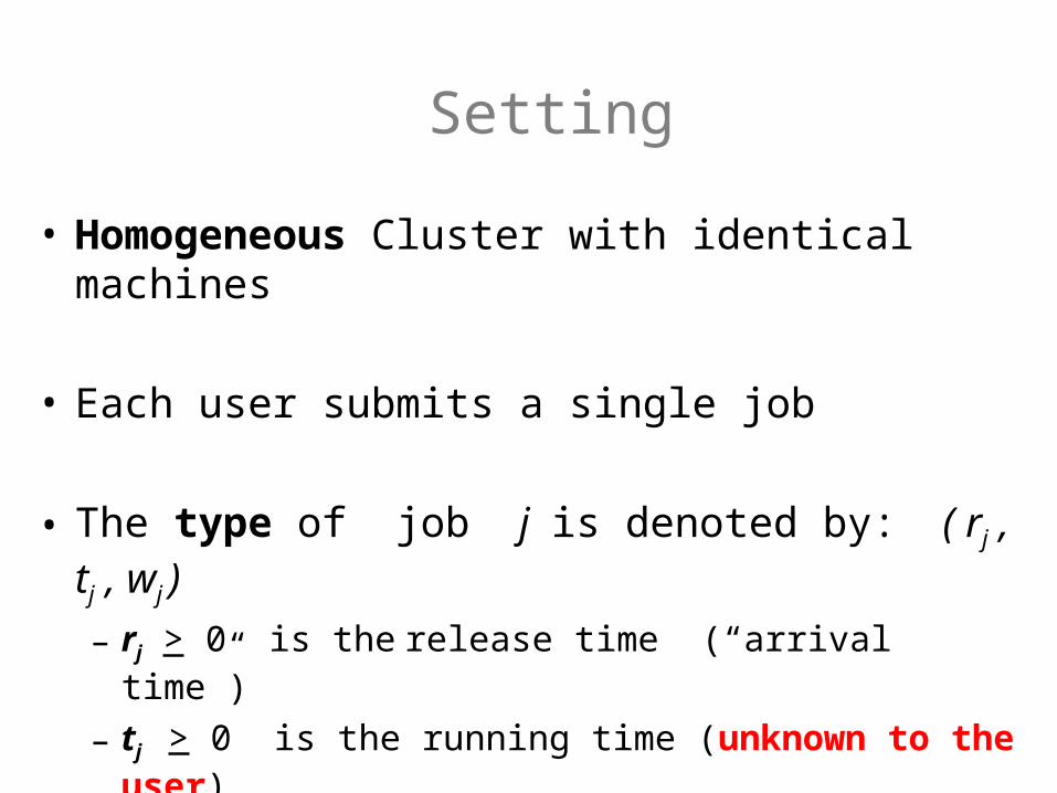
• Homogeneous Cluster with identical machines

• Each user submits a single job

• The type of job j is denoted by: ( rj , tj , wj )

– rj > 0 is the release time (“arrival time”)

– tj > 0 is the running time (unknown to the user)

– wj > 0 is the value per unit time of delay

Setting

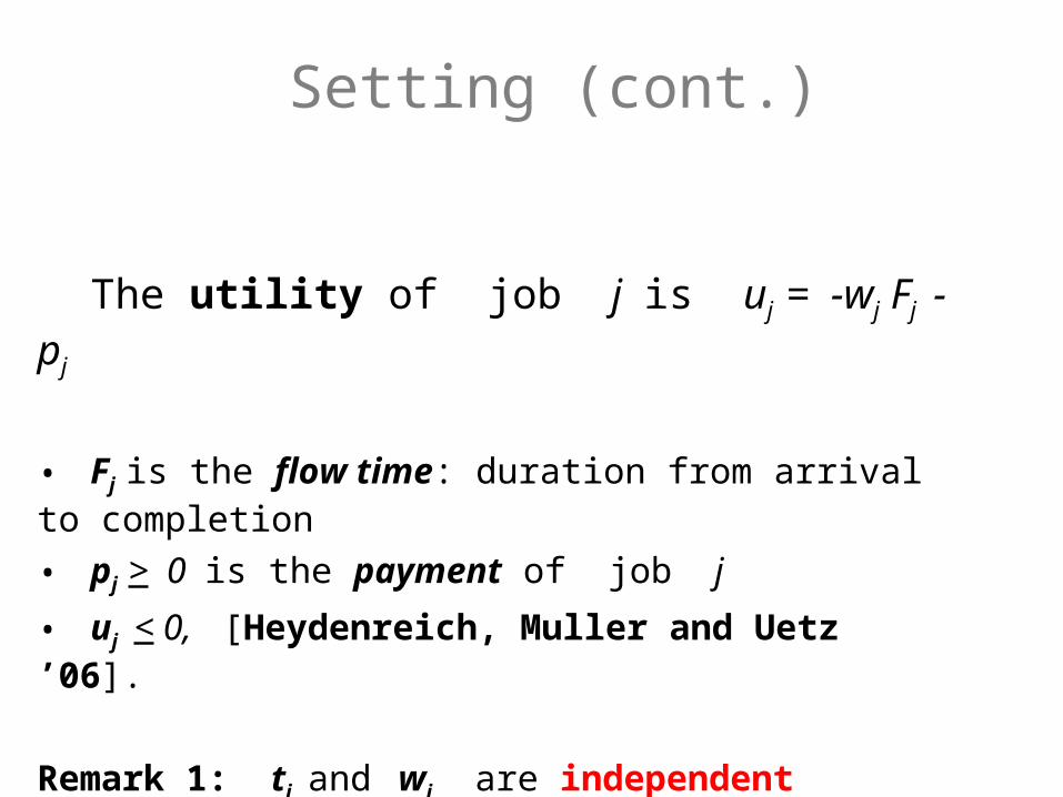
The utility of job j is uj = -wj Fj - pj

• Fj is the flow time: duration from arrival to completion

• pj > 0 is the payment of job j

• uj < 0, [Heydenreich, Muller and Uetz ’06].

Remark 1: tj and wj are independent

Remark 2: to generate wj we used a bimodal distribution

Setting (cont.)

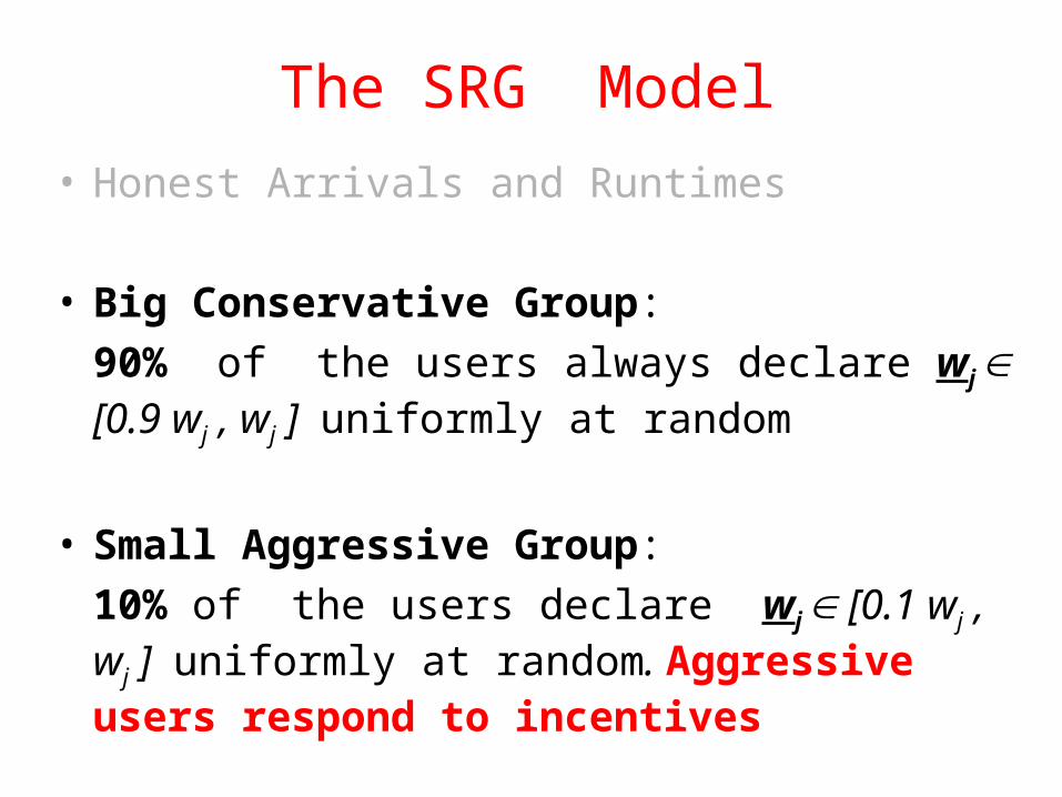
The SRG Model

• Honest Arrivals and Runtimes

• Big Conservative Group:

90% of the users always declare wj [0.9 wj , wj ] uniformly at random

• Small Aggressive Group:

10% of the users declare wj [0.1 wj , wj ] uniformly at random. Aggressive users respond to incentives

► Stability Analysis

We formulate a simple one-shot game to model the dynamic interaction between the provider and an aggregate consumer playing on behalf of the aggressive users

We then look for a Nash-equilibrium in this restricted game

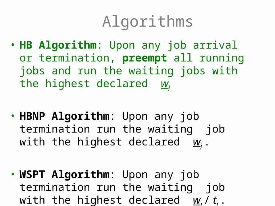
• HB Algorithm: Upon any job arrival or termination, preempt all running jobs and run the waiting jobs with the highest declared wj

• HBNP Algorithm: Upon any job termination run the waiting job with the highest declared wj .

• WSPT Algorithm: Upon any job termination run the waiting job with the highest declared wj / tj . – Remark: WSPT has informational advantage by

knowing tj.

Algorithms

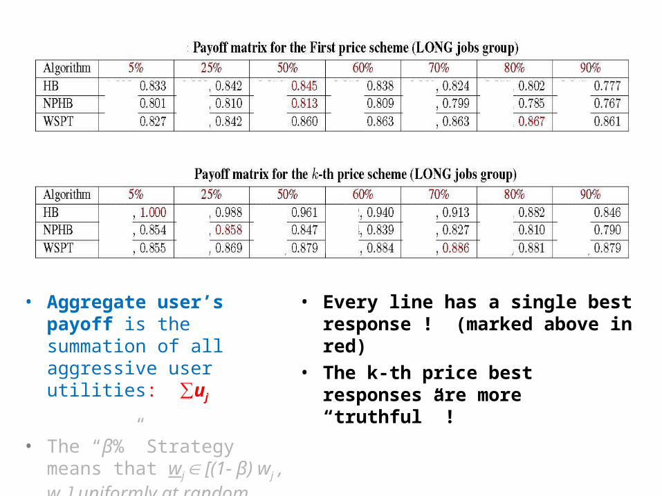
• Aggregate user’s payoff is the summation of all aggressive user utilities: ∑uj

• The “β%” Strategy means that wj [(1- β) wj , wj ] uniformly at random.

• Every line has a single best response ! (marked above in red)

• The k-th price best responses are more “truthful” !

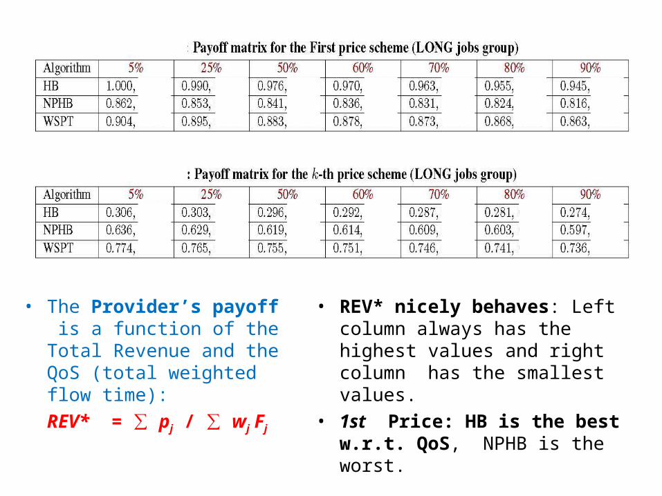
• The Provider’s payoff is a function of the Total Revenue and the QoS (total weighted flow time):

REV* = ∑ pj / ∑ wj Fj

• REV* nicely behaves: Left column always has the highest values and right column has the smallest values.

• 1st Price: HB is the best w.r.t. QoS, NPHB is the worst.

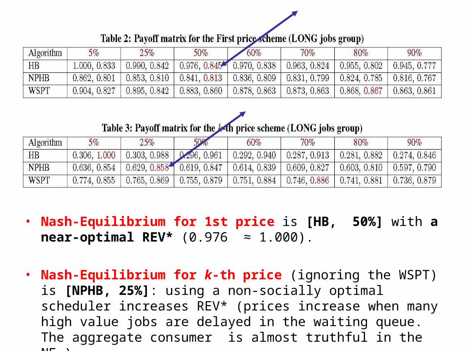
• Nash-Equilibrium for 1st price is [HB, 50%] with a near-optimal REV* (0.976 ≈ 1.000).

• Nash-Equilibrium for k-th price (ignoring the WSPT) is [NPHB, 25%]: using a non-socially optimal scheduler increases REV* (prices increase when many high value jobs are delayed in the waiting queue. The aggregate consumer is almost truthful in the NE ).

• We introduced the SRG Model: a simple behavioral model to study scenarios with inherent uncertainties.

• We modeled the dynamic on-line interaction between the provider and consumers as a one shot game and showed the existence of (arguably good) unique ‘pure’ symmetric Nash Equilibrium.

• Future Work: – Non-linear value and utility models.– Strategic impact of budgets (runtime uncertainty causes

unpredicted payments).– Competition among providers in a more direct manner.

Conclusions (Empirical Part)

Thank You