Contemporary Mathematics Volume 114, 1990

On Solving the Linear Programming Problem Approximately

NIMROD MEGIDDO

ABSTRACT. This paper studies the complexity of some approximate solutions of linear programming problems with real coefficients.

1. Introduction

The general linear programming problem is to maximize a linear func- tion over a set defined by linear inequalities and equations. There are many equivalent ways to represent instances of the linear programming problem. For example, consider the symmetric form

Maximize cTx (SyN-4 , b , c)) subject to Ax 5 b

x 2 0 .

The dual is then

Minimize b ' y subject to A * ~ 2 c

Y 2 0 .

Intuitively, two representations are equivalent if there is an easy way to transform solutions of one to solutions of the other and vice versa. We first mention some of the well-known equivalences. First, any set of linear inequalities and linear equations can be reduced to a set of linear equations with nonnegativity constraints or to a set of inequality and nonnegativity constraints. Also, any linear programming problem can be reduced to a linear programming problem with a nonempty set of solutions by using artificial variables. Moreover, any linear programming problem can be reduced to a problem of finding a solution to a system of linear inequalities (by combining the constraints of the primal and dual and adding the inequality cTx 2 b T y )

1980 Mathematics Subject Classification (1985 Revision). Primary 90C05.

@ 1990 American Mathematical Society 0271-4132190 $1.00 + $.25 per page

3 5

36 NIMROD MEGIDDO

or else concluding that the system has no solution. By the duality theorem, if we put the problem in the combined primal-dual form, every problem can be reduced to a problem that is either infeasible or feasible and bounded (but not unbounded). It is interesting to note that over any ordered field, every linear programming problem can be reduced to one that is both feasible and bounded. This is done as follows. Suppose the problem is given in the symmetric form Sym(A , b , c) . Consider the following:

Minimize cTx - b Ty +t subject to Ax - te 5 b

A ~ Y + te 2 c T c x - b T y 2 0

x , y , t L O , where e denotes a vector of 1's. It is easy to verify that the optimal value of the latter is zero if and only if the former has an optimal solution. In this case the latter provides optimal solutions for the former and its dual.

The equivalences mentioned above are valid as long as exact computation is feasible. In practice one usually works with finite precision and hence obtains results that are only "approximately true." However, the meaning of the last sentence depends on the particular representation of the practical problem. Indeed, a good approximate solution for one representation of the problem may transform into a very bad approximate solution for another "equivalent" representation of the same problem.

When two people talk about approximate solutions, they often think of different notions of approximation. It is quite likely though that they refer to one of the following:

(i) A feasible point (i.e., one that satisfies all of the constraints in the exact sense) and is close in a certain metric to an optimal point.

(ii) A feasible solution whose objective function value is close to the optimal value.

(iii) A point, not necessarily feasible, close to an optimal solution. (iv) A point that approximately satisfies every constraint, and whose ob-

jective function value is close to the optimal value. (v) A point close to the feasible domain, whose objective function value

is close to the optimal value (called the "weak optimization problem" in [7]).

(vi) A basis where the simplex algorithm (using exact arithmetic) termi- nates, but the numerical values of variables are only approximate.

(vii) A basis where the simplex algorithm terminates due to a prescribed tolerance.

The choice of the right definition depends very much on the practical situation. In fact, practical considerations dictate which constraints must be satisfied and which may be approximately satisfied. In other words, the tolerance may be different for different constraints.

ON SOLVING THE LINEAR PROGRAMMING PROBLEM APPROXIMATELY 37

It is not known whether the m x n linear programming problem with real data can be solved in a polynomial number of arithmetic operations and com- parisons in terms of m and n . (We will refer to this notion of complexity as strongly polynomial time, even though the usual definition of this con- cept also requires polynomial time in the usual sense.) Thus, another natural question is whether for any E > 0 , any of the &-approximation problems can be solved in a polynomial number of operations in terms of m , n , and -log&. To deal with this question, we first have to define what we mean by an "&-approximate" solution. In particular, such a definition should not make the second question trivially equivalent to the first one. Consider, for exam- ple, the concept suggested in (i) above. Thus, for the problem Maximize cTx subject to Ax 5 b (assuming its maximum V* exists) an &-approximate so- lution is a point x such that Ax < b and cTx > V* - E . This definition is not satisfactory since it is not clear whether an &-approximation algorithm is required to decide the existence of an x such that Ax < b , and the bound- edness of the function cTx on the feasible domain. If indeed it is required to decide these questions, then in the worst-case sense this approximation problem is trivially equivalent to the exact problem.

The consequences of the ellipsoid algorithm with respect to approximation problems on convex sets are studied in [7]. It is not clear whether these results can be applied to achieve the type of results we seek here. The reason is that over the real numbers it seems difficult to obtain estimates of the radii of a circumscribing sphere and an inscribed sphere. The main complexity result on convex minimization in [7] (Theorem 2.2.15) assumes that the convex set is given with estimates of such radii. Our main interest here is the question of what is a reasonable sense of approximation when the algorithm fails to classify the instance correctly as feasible, unbounded, etc.

In Section 2 we give some preliminaries and discuss the difficulties involved in classifying the problem. In Section 3 we discuss approximate solutions based on satisfying a termination criterion within some tolerance. In Section 4 we discuss a notion of approximation that is based on solving a perturbed instance exactly. Section 5 gives an analysis of complexity for various notions of complexity.

2. Preliminaries

We pointed out in the introduction that the practical situation usually dictates the right notion of approximate solution. For a theoretical discus- sion it is often convenient to consider the problem in the symmetric form Sym(A , b , c) . (See Section 1.) Traditionally, an exact algorithm for this problem (for example, the simplex method) is supposed to provide the user with information as follows. It has to classify the problem into one of the following three categories:

(i) Infeasible. (The domain X defined by Ax 5 b and x 2 0 is empty.)

NIMROD MEGIDDO

(ii) Feasible and bounded. (There exists a maximizer of c T x over X .) (iii) Feasible and unbounded. (The function cTx is unbounded over X .)

In case (ii) the algorithm has to provide an optimal solution. The algorithm may also be required in case (iii) to provide a ray contained in X along which c T x tends to infinity. A nice property of the simplex method is that it also solves the dual problem

Minimize b T y subject to > c

Y 10. Thus, besides providing such a ray in case (iii), the algorithm also provides in case (ii) an optimal solution to the dual, and in case (i) a "certificate" in the form of a ray of a related problem.

In fact, the (exact) simplex method always computes a basis that provides the required information. Specifically, it provides a representation of the problem (by a suitable linear transformation of the space) from which the classification and the numerical values of both the primal and the dual vari- ables are transparent. Thus, the simplex method classifies problems into one of four categories (even though the commonly used variants do not distin- guish between IF and 11):

(i) FF: primal feasible, dual feasible. (ii) FI: primal feasible, dual infeasible (that is, unbounded primal).

(iii) IF: primal infeasible, dual feasible (here the dual is unbounded). (iv) 11: primal infeasible, dual infeasible.

It is quite common to include this classification in the requirements from an exact algorithm for the general linear programming problem. We refer to it later as the classification problem of linear programs.

An approximation algorithm should be expected sometimes to fail in clas- sifying the input into the categories FF, FI, IF, and 11. Interestingly, the existence of a strongly polynomial algorithm for the classification problem implies the existence of one for the problem itself. (See page 445 in [I].)

So far we have discussed the subject of approximation under the assump- tion that the result should be "close" to the true one. However, a different approach can sometimes be useful. We may allow the algorithm to be totally wrong in a small number of cases. This approach is approximate when the output space of the algorithm is discrete and has no natural metric associated with it. For example, consider the following trivial problem: Given two num- bers a , p , recognize whether a > /3 or a 5 /3. Suppose the comparison of a to p can be performed with arbitrary finite precision. Thus, for any given E > 0, we can recognize either that

or that

ON SOLVING THE LINEAR PROGRAMMING PROBLEM APPROXIMATELY 39

The algorithm reports a 5 P in the first case and a 2 P in the second one. Thus, the algorithm gives the correct answer if

but may fail otherwise. The grey area is the set of pairs ( a , P) such that la: - PI 5 E . Of course, the smaller E the smaller the grey area. Thus, the measure of the grey area reflects the quality of the approximation.

The problem of the preceding paragraph can be cast as a linear program- ming problem

Maximize x, subject to ax, 5 x, 5 f ix, .

Here the point (0, 0) is feasible for any a and P . The problem is un- bounded if and only if a 5 /3 . This suggests that the grey area approach would be suitable for the classification problem of linear programs.

A general linear programming problem in standard form Maximize crx

(SF@, b , c)) subject to Ax = b x 1 0

is determined by A E RmX" , b E Rm , and c E R" . There is a one-to- one correspondence between problems of order m x n and points of R =

R~"+"'+" . The classification corresponds to a partition of R into four sets: FF, FI, IF, and 11, as discussed above. For example, IF is the set of triples (A, b , c) that determine infeasible primal problems whose dual problems are feasible (and hence unbounded).

Let R' denote the union of the boundaries of these four sets. Obviously, an approximation algorithm (for the classification problem) may fail if the input (A, b , c) is close to R' . For example, if an instance is close to the common boundary of FF and FI, but far from the boundaries of IF and 11, then an approximation algorithm is expected to recognize that the prob- lem is feasible, but is expected to fail in deciding whether it is bounded. Interestingly, there are more "pathological" cases. In fact, the intersection of all four boundaries, which we denote by R, , is not empty. Thus, given an instance close to the intersection of the four boundaries, an approxima- tion algorithm may not be able to recognize anything in terms of the above classification. This observation is obvious in view of the invariance of the classification under multiplication of columns and rows by positive scalars. Thus, the neighborhood of the origin is obviously pathological in this sense. The difficulties with the origin can be avoided by scaling rows and columns. However, it is easy to construct other examples with similar characteristics.

PROPOSITION 2.1. The instance Maximize x, - x, subject to x, - X, 5 - 1

(*I -x, + X 2 5 - 1

x , , x 2 2 0 . belongs to Q, .

40 NIMROD MEGIDDO

PROOF. It is easy to see that (*) itself is in IF. Using small perturbations, one can move from (*) to instances in any of the other three classes. More precisely, if only c, is slightly increased then we can get instances in 11. If only A,, is slightly decreased then we get instances in FF. Finally, if only A , , is slightly increased then an instance in FI is obtained.

We note that most of the numerical difficulties in solving linear program- ming problems are due to the fact that many such problems are ill posed. It is well known in numerical analysis (see, e.g., [3]) that near-singularities in the matrix A can cause problems. However, in this paper we also discuss in- trinsic aspects of approximate solutions that arise even when exact arithmetic is used. For example, if one is interested only in an approximate solution, what should be a good termination criterion? Because of such questions we have to deal with perturbations of the vectors b and c and not only of the matrix A .

Due to the classification aspect of the problem, we clearly cannot always measure the quality of the approximation by the distance between the exact solution and the approximate one (neither in terms of the solution vector nor in terms of the objective function value). Thus a different approach to approximation may be proposed for a general situation, where there is some natural metric on the input space, but there does not seem to exist one for the output space. The following definition is similar to backward analysis of errors in numerical analysis [9 ] .

DEFINITION 2.2. Let M = (S , d ) be a metric space and let f be a map- ping from S into some set T that does not necessarily have any metric associated with it. A mapping g : S 4 T is called an E-approximation to f if for every x E S , there exists an x' E S such that d(x , x') < E and g(x) = f (x').

In linear programming the output space (including the classification) does have a metric structure. Besides the classification information, there are also numerical values associated with the variables. One might propose for the linear programming problem the following approach to approximation by posing the following problem:

PROBLEM 2.3. Given the problem SF(A , b , c) and E > 0, name a class S E {FF, FI , IF, 11) and assign numerical values to the variables so that the following condition is satisfied: There exists an instance (A', b' , c') in S for which the numerical values are correct within an error of E . such that IIW, b , C ) - ( A ' , b' , cl)II, < E -

The approach represented by Problem 2.3 takes care of pathological cases where some other approaches fail. Consider, for comparison, a different notion of approximate solution of systems of inequalities reflected in the following problem:

PROBLEM 2.4. Given A , b and E > 0, either give an x such that Ax 5 b + ee or conclude that there is no x such that Ax 5 b - ee .

ON SOLVING THE LINEAR PROGRAMMING PROBLEM APPROXIMATELY 4 1

The approach represented by Problem 2.4 seems to be a natural gener- alization of the obvious approximate comparison of two real numbers. Its weakness is apparent in the following example. Consider the problem

If a = 1 then, obviously, for every E < 1 the system

is infeasible. However, for any a # 1 the system is feasible for every & . Thus, in order to solve Problem 2.4 we have to know whether a = 1 . This example can easily be generalized so that in order to solve Problem 2.4 one has to know whether a certain matrix is singular. The latter involves some numerical difficulties in practice.

The weakness of the concept of Problem 2.4 is that it considers pertur- bations of the given problem only in a limited and quite arbitrary way. In Problem 2.3 we allow perturbations in all directions. We note that for cer- tain classes of linear programming problems (e.g., the min-cost flow problem) certain coefficients have the values 1 or 0 throughout the class. In such cases we would allow only perturbations within the subject class. Thus, if the con- cept represented by Problem 2.3 were to apply to a min-cost flow problem SF(A , b , c) then we would require that A' = A .

3. Tolerance-based approximation

In this section we discuss the issue of approximation as it arises in the context of the simplex method. There are two ways to look at the question. First, imagine we run the simplex algorithm using exact arithmetic but have to compute only "e-approximate" solutions. Thus, rather than running the algorithm to the end, we seek to apply some stopping rule that guarantees our output to be &-approximate. The interesting problem is of course to devise such stopping rules for various concepts of approximation. Another way to look at the question is to realize that on a machine we usually have numerical errors, and thus we almost always have to specify some "tolerance" within which we accept our results. It is important to know the implications of using a certain tolerance with regard to the results.

Consider the problem SF(A, b , c) . In the Appendix we review some properties of basic solutions and how the simplex method uses them. (See the Appendix for the notation.)

In practice, one usually works with some "tolerance" 6 > 0, so that any number a 5 6 is accepted as nonpositive and any a 2 -6 is accepted as nonnegative. This suggests another approach to approximation, which may

42 NIMROD MEGIDDO

be called the "tolerance" approach: DEFINITION 3.1. A basic solution x = x(B) = (x,, x,) (where xB =

B-' b and xN = 0) is optimal with tolerance 6 for SF(A , b , c) if for every j ,

T -1 x > -6 and cj <c,B A j + 6 . J -

Obviously, such a solution is not necessarily feasible. It is only "approxi- mately feasible" in the sense that the equality constraints are satisfied while the nonnegativity constraints are approximately satisfied. Analogously, the dual vector y(B) is approximately feasible in the dual problem. Moreover, the vectors x(B) and y(B) satisfy the complementary slackness condition

T xj(y A. - c . ) = 0 ,

I I

which is necessary for optimality. This implies that both vectors yield the same objective function value in their respective problem

T T -1 T c x = c B b = y b .

Note that the problem may also be feasible and unbounded but that an op- timal solution with tolerance 6 may still exist. One can also define a notion of an unbounded ray with tolerance 6 .

4. Perturbation-based approximation

It is interesting to observe that from a solution that is optimal with small tolerance we can easily obtain an exact solution to an instance that is close to the given one. More precisely, we have the following proposition:

PROPOSITION 4.1. Suppose x = x(B) is a basic solution that is optimal with tolerance 6 . Let x' be defned by xi = xj + 6 for j associated with B and xj = 0 otherwise. Also, let c' be defined by c; = cI for j associated with B and c: = c, - 6 otherwise, and let b' = b + 6Be. Under these conditions, x' is an optimal solution for the problem SF(A , b' , c') , and y = B - ~ c , is optimal for its dual problem.

PROOF. We have x b = ~ - l b ' = x , + ~ e > O ,

> c'

and x' and y satisfy the complementary slackness conditions required in SF(A , b' , c') . 0

In simpler words, we have

COROLLARY 4.2. If x is optimal with tolerance 6 for SF(A , b , c) then there exist b' and c' and an optimal solution x' for SF(A , b' , c') such that

lb' - 41, 3 llc' - 4, 5 6 9

and llb' - bll, 5 min{GIIAJI,, m T 6 )

ON SOLVING THE LINEAR PROGRAMMING PROBLEM APPROXIMATELY 43

where 1 1 All, is the usual operator norm, corresponding to the vector supremum norm 1 1 . 1 1 , T is the maximum absolute value of any entry in A , and m is the number of rows of A .

A analogous proposition can be proven with respect to the unbounded case:

PROPOSITION 4.3. Suppose x = x ( B ) is a basic solution such that

and for some k not associated with B ,

and B-'A, 2 - 6 1 .

Let c' be the same as e except that cl = c, + d c i e , and let b' = b + SBe . Also, let A' be the same as A except that A; = A, + 6 B e . Under these conditions, the problem SF(A' , b' , c ' ) is unbounded.

PROOF. In the new problem the basis B certifies unboundedness since

and

COROLLARY 4.4. If SF(A , b , c ) is concluded within tolerance 6 to be unbounded, then there exist A' , b' , and c' such that SF(A' , b' , c') is un- bounded,

I IA ' - All, 5 JllAllm (where 11~'- All is the operator norm corresponding to the vector norm 1 1 . 1 1 I ) ,

5. Complexity questions

We start this section with yet another variant of an approximation prob- lem. Again, we consider approximation concepts that avoid the difficulties involved in the classification problem. Suppose the exact problem is given in the dual form

Minimize c T x subject to Ax 2 b

where the output has to be one of the following:

(i) a point x* that minimizes c T x subject to Ax > b ,

NIMROD MEGIDDO

(ii) a point x* and a scalar t* > 0 that minimize the value of t subject to Ax + te 2 b (in which case the problem is infeasible), or

(iii) vectors x and u such that Ax 2 b , cTu < 0 , and Au 2 0 (in which case the problem is unbounded).

The above motivates the definition of the following approximation problem: PROBLEM 5.1. Denote the optimal value of a given problem DF(A , b , c)

by V* (allowing V* = f o o ) and let t* denote the minimum of t subject to Ax + te 2 b . Given a number E > 0 , output one of the following:

(i) a point x such that cTx < V* + E and Ax 2 b - ee , (ii) apoint x andascalar t , -e I t 5 t*+e suchthat Ax+te 2 b-ee,

or (iii) vectors x and u such that Ax 2 b - ee , cTu < E , and Au 2 -ee . It is interesting to look at the question of the existence of an algorithm for

the approximation problem, where the number of operations is expressed in terms of E as well.

PROPOSITION 5.2. Over any ordered jield, if Problem 5.1 can be solved in f (m , n , e) field operations (including comparisons) then it can be solved in g(m , n) = O( f (m , n , 1)) operations.

PROOF. Suppose d is an algorithm for Problem 5.1 that runs in f (m , n , E ) field operations. Given A , b , c and e > 0 , let

- - The instance DF(A , b , Z) is equivalent to DF(A , b , c) . Moreover, a valid - - output for DF(A , b , 5) with precision e = 1 is also a valid output for DF(A , b , c) with the prescribed precision e .

COROLLARY 5.3. If there exists a polynomial f (m , n , c) such that Prob- lem 5.1 with rational data can be solved in f (m , n , e) arithmetic operations, then the exact problem with rational data can be solved in a polynomial num- ber of operations.

PROOF. For a problem with rational data it is easy to determine a value c such that an exact solution can be computed from a solution of Problem 5.1 in a polynomial number of operations. Thus, the problem can be scaled so that e = 1 suffices for determining an exact solution. 0

In view of Proposition 5.2 it is reasonable to ask whether Problem 5.1 can be solved in a polynomial number of operations in terms of m , n , and log R/e , where R = R(A , b , c) > 0 is some quantity such that for any positive scalar I

R(IA , Ab , Ic ) = IR(A , b , c)

(e.g., R equals the maximum absolute value of any input coefficients).

ON SOLVING THE LINEAR PROGRAMMING PROBLEM APPROXIMATELY

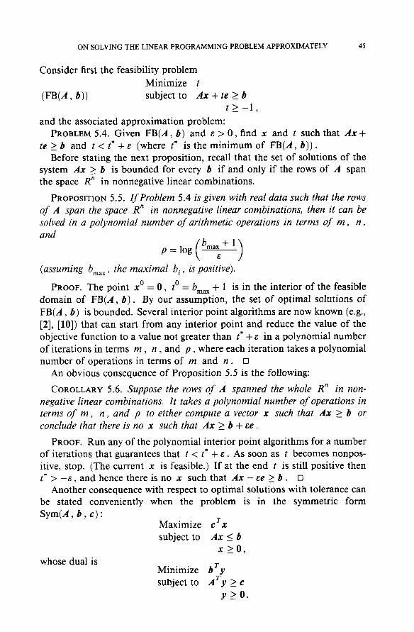
Consider first the feasibility problem Minimize t

(FB(A , b ) ) subject to Ax + te L b t 2 - 1 ,

and the associated approximation problem: PROBLEM 5.4. Given FB(A , b ) and E > 0 , find x and t such that Ax +

te 2 b and t < t* + E (where t* is the minimum of FB(A, 6 ) ) . Before stating the next proposition, recall that the set of solutions of the

system Ax > b is bounded for every b if and only if the rows of A span the space Rn in nonnegative linear combinations.

PROPOSITION 5.5. If Problem 5.4 is given with real data such that the rows of A span the space R" in nonnegative linear combinations, then it can be solved in a polynomial number of arithmetic operations in terms of m , n , and

(assuming bmax, the maximal bi , is positive). 0 0 PROOF. The point x = 0 , t = bmax + 1 is in the interior of the feasible

domain of FB(A , b ) . By our assumption, the set of optimal solutions of FB(A , b ) is bounded. Several interior point algorithms are now known (e.g., [2], [lo]) that can start from any interior point and reduce the value of the objective function to a value not greater than t* + E in a polynomial number of iterations in terms m , n , and p , where each iteration takes a polynomial number of operations in terms of m and n . 0

An obvious consequence of Proposition 5.5 is the following:

COROLLARY 5.6. Suppose the rows of A spanned the whole R" in non- negative linear combinations. It takes a polynomial number of operations in terms of m , n , and p to either compute a vector x such that Ax 2 b or conclude that there is no x such that Ax b + ~e .

PROOF. Run any of the polynomial interior point algorithms for a number of iterations that guarantees that t < t* + E . As soon as t becomes nonpos- itive, stop. (The current x is feasible.) If at the end t is still positive then t* > - E , and hence there is no x such that Ax - Ee 2 b . 0

Another consequence with respect to optimal solutions with tolerance can be stated conveniently when the problem is in the symmetric form Sym(A , b , c) :

Maximize cTx subject to Ax 5 b

x LO, whose dual is

Minimize b Ty subject to 2 c

Y 2 0 .

46 NIMROD MEGIDDO

Recall that by the duality theorem, a feasible solution x is optimal if and only if there exists a dual feasible solution y such that cTx = bTy . On the other hand, c 'x 5 bTy for any pair of feasible x and y . This suggests the following approximation problem:

PROBLEM 5.7. Given A, b , c and E > 0 , either find a pair of vectors x , y such that

Ax 5 b +ee , T

A y Z c - ~ e , T T b y - c X ~ E ,

x 2 - & e , y > - & e

or conclude that Sym(A, b , c) does not have an optimal solution. The notion of approximation presented in Problem 5.7 is very close to the

one used in practice, where optimality criteria are applied without knowledge of proximity to the value of an optimal solution.

Note that Problem 5.7 is trivial if c 5 0 I b . Thus, assume

and denote

PROPOSITION 5.8. Suppose the rows of the matrix

r o ~~1

span the space R"'" in nonnegative linear combinations. Problem 5.7 can be solved in a polynomial number of operations in terms of m , n , and p* .

PROOF. Consider the problem Minimize t subject to A x - t e i b

+ te 2 c b T y - c T x - t I O x + t e , y + t e L O .

Starting at t = y + 1 , x = 0 , and y = 0 , run a number of iterations that guarantees t 5 t* + E . This number is polynomial in m , n , and p* , and p* is trivial to compute. If t 5 E then the current x and y solve Problem 5.7. Otherwise, t* > 0 , and Sym(A , b , c) does not have an optimal solution.

Note that a solution of Problem 5.7 does not guarantee that cTx is close to the optimal value V* when the latter exists. It seems much more dif- ficult to solve the approximation problem in the latter sense. This diffi- culty can be explained by considering the following practical question, which

ON SOLVING THE LINEAR PROGRAMMING PROBLEM APPROXIMATELY 47

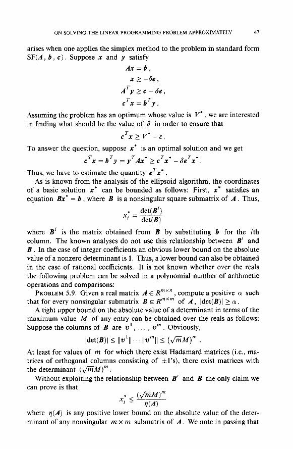
arises when one applies the simplex method to the problem in standard form SF(A , b , c) . Suppose x and y satisfy

A x = b ,

x 2 -6e,

Assuming the problem has an optimum whose value is V* , we are interested in finding what should be the value of 6 in order to ensure that

To answer the question, suppose x* is an optimal solution and we get

Thus, we have to estimate the quantity eTx* . As is known from the analysis of the ellipsoid algorithm, the coordinates

of a basic solution x* can be bounded as follows: First, x* satisfies an equation Bx* = b , where B is a nonsingular square submatrix of A . Thus,

where B' is the matrix obtained from B by substituting b for the ith column. The known analyses do not use this relationship between B' and B . In the case of integer coefficients an obvious lower bound on the absolute value of a nonzero determinant is 1. Thus, a lower bound can also be obtained in the case of rational coefficients. It is not known whether over the reals the following problem can be solved in a polynomial number of arithmetic operations and comparisons:

PROBLEM 5.9. Given a real matrix A E R"'" , compute a positive a such that for every nonsingular submatrix B E R"'"' of A , Idet(B)I L a .

A tight upper bound on the absolute value of a determinant in terms of the maximum value M of any entry can be obtained over the reals as follows: Suppose the columns of B are v ' , . . . , v m . Obviously,

At least for values of m for which there exist Hadamard matrices (i.e., ma- trices of orthogonal columns consisting of f l's), there exist matrices with the determinant ( \ / T i i ~ ) ~ .

Without exploiting the relationship between B' and B the only claim we can prove is that

* ( f i W r n xi < rtw where q(A) is any positive lower bound on the absolute value of the deter- minant of any nonsingular m x m submatrix of A . We note in passing that

48 NIMROD MEGIDDO

in the case of integral coefficients the bounds on xf cannot be improved dramatically. For example, if

and b = (1, 0, .. . , 0)' then x i = l / ( M ( M + I ) ~ - ' ) . Recall that to guarantee an &-approximation in terms of the function value,

we have to choose 6 such that

and b = ( M , ... , M)' then x i = zEl M'. Also, if

Hence we get the estimate

B =

Another estimate can be derived by

- M M M . . . M - -1 M M . . . M

-1 M . . . M

. . -1 M -

where Amin denotes the least eigenvalue. Thus, what we would need is a lower bound on the least eigenvalue of any matrix of the form BBT where B is a basis. Note that our estimates depend on properties of an optimal basis rather than one that supports the approximate solution. So, the optimal basis may be ill conditioned, this fact being unknown to the user, and the terminal basis well conditioned and satisfying the optimality conditions within tolerance.

Obviously, if any q(A) is known then we can solve the &-approximation problem in a polynomial number of operations in terms of m , n , and - log6 . However, in general y is not known. It is interesting to note that for a practical solution of problems with thousands of variables, even with a sparse and well-structured problem with small integral coefficients, the re- quired 6 may be too small to be practical. It is not clear that an approximate solution based on tolerance has a value close to the optimal. In fact, the value may be far from the optimum even though the duality gap is very small, since the vectors x and y are only approximately feasible.

ON SOLVING THE LINEAR PROGRAMMING PROBLEM APPROXIMATELY 49

The following example illustrates the difficulties described above. Suppose we solve a problem in standard form, and the representation using the current basis is T Maximize i.,x, -

subject to x, + N x , = e

where fi E R " ' ~ ( " - ~ ) contains the following m x m submatrix:

Suppose further that the coordinates of i., are negative except for those corresponding to the columns of B' that are all equal to zero except for the last one, which equals 1 0-20 . Suppose m = 1000, which is quite common in practice. Assuming is considered nonpositive within tolerance, the solution x = e is accepted as optimal, with an objective function value of 0. However, the basis B' determines a feasible solution x where x,, = 2' - 1

and the objective function value is greater than . Note that the current basis B is very well conditioned. Moreover, the underlying matrix is very sparse and well structured.

Appendix

We review some known characteristics of the simplex method for problems in standard form SF(A , b , c ) . Suppose, for simplicity, we run only "phase 11" of the algorithm; i.e., we start from a basic feasible solution and attempt to find an optimal one or conclude that the problem is unbounded. (It is well known that if a problem in standard form has a feasible solution then it has a basic feasible one; the "phase I" problem of finding a basic feasible solution, or concluding that none exists, can be formulated as a problem in standard form with a known basic feasible solution.) Assuming exact arithmetic, the algorithm then terminates with a feasible basis. The termination criterion is stated in terms of signs of certain entries of the "tableau." As is common, let B E RmXm denote the nonsingular submatrix of A whose columns con- stitute the current basis, and let N denote the matrix consisting of the other columns. Let x, and c, denote the restrictions of the vectors x and c , respectively, to the indices corresponding to the columns of B . Let x, and c, denote the complementary restrictions of the vectors. The "tableau" is essentially a representation of the problem in an equivalent form:

T T - 1 Maximize (c, - c, B N ) x , subject to X, + B-' NX, = B-' b

x, 2 0 , x, 2 0 .

50 NIMROD MEGIDDO

Given a basis B , the corresponding basic primal solution x = x(B) is given by

x,=B-lb, x,=O.

The basic dual vector y = y(B) associated with B is given by the equation

The dual problem is Minimize T b subject to y T ~ 2 cT .

Thus, y(B) is feasible in the dual problem if and only if

in which case y is optimal for the dual. Assuming that the algorithm (namely, the primal simplex method) works

with exact arithmetic, for every B occurring in the process,

The algorithm terminates in one of the following cases: T T -1

(i) c, 5 c, B N , in which case B is optimal, or T -1 (ii) there exists a column N, such that c, > c, B N, and B-' N, 5 0 ,

in which case the problem is unbounded.

In either case the basis B is said to be terminal. The termination criterion applies to signs of certain entries in the tableau.

1. V. Chvatal, Linear programming, W. H. Freeman, New York, 1983. 2. D. M. Gay, A variant of Karmarkar's linear programming algorithm for problems in

standard form, Math. Programming 37 (1 987), 8 1-90. 3. G. H. Golub and C. Van Loan, Matrix computations, Johns Hopkins University Press,

1983. 4. C. C. Gonzaga, Polynomial afine algorithms for linear programming, Report ES-139188,

Dept. of Systems Engineering and Computer Sciences, COPPE, Rio de Janeiro, 1988. 5. M. Grotschel, L. Lovasz, and A. Schrijver, The ellipsoid method and its consequences in

combinntorial optimization, Combinatorica 1 (1 98 I), 169- 197; Corrigendum: Combina- torica 4 (1984), 291-295.

6. L. G. Khachiyan, A polynomial algorithm in linear programming, Soviet. Math. Dokl. 20 (1979), 191-194.

7. L. Lovasz, An algorithmic theory of numbers, graphs and convexity, SIAM, Philadelphia, 1986.

8. N. Megiddo, Combinatorial optimization with rational objectivefunctions, Math. Oper. Res. 4 (1979), 414-424.

9. J. H. Wilkinson, Error analysis offloating-point computation, Numer. Math. 2 (1960), 2 19-340.

10. Y. Ye and M. Kojima, Recovering optimal dual solutions in Karmarkar's polynomial algorithm for linear programming, Math. Programming 39 (1987), 305-317.

IBM RESEARCH DIVISION, ALMADEN RESEARCH CENTER SAN JOSE, CALIFORNIA 95 120-6099, AND SCHOOL OF MATHEMATICAL SCIENCES, TEL AVIV UNIVERSITY, TEL AVIV, ISRAEL

E-mail address : MEGIDDO@IBM.COM