on some classes of discrete polynomials and ordinary ... · on some classes of discrete polynomials...
TRANSCRIPT
arX
iv:1
308.
5018
v3 [
nlin
.SI]
24
Mar
201
4
On some classes of discrete polynomials and
ordinary difference equations
Andrei K Svinin
Institute for System Dynamics and Control Theory, Siberian Branch of Russian
Academy of Sciences, Russia
E-mail: [email protected]
Abstract. We introduce two classes of discrete polynomials and use them for
constructing ordinary difference equations admitting a Lax representation in terms
of these polynomials. We also construct lattice integrable hierarchies in their explicit
form and show some examples.
PACS numbers: 02.30.Ik
Keywords: KP hierarchy, integrable lattices
Submitted to: J. Phys. A: Math. Theor.
1. Introduction
A discrete counterpart of an Nth order autonomous ordinary differential equation is a
recurrence relation of the form
T (i+N) = F (T (i), T (i+ 1), . . . , T (i+N − 1)) (1)
for an unknown function T (i) of a discrete variable i ∈ Z. One calls (1) an ordinary
discrete (difference) equation of Nth order. Equation (1) yields a map RN → R
N for
real-valued initial data {yj ≡ T (i0 + j) : j = 1, . . . , N − 1}. By analogy with ordinary
differential equations, the function J = J(i) = J(T (i), T (i + 1), . . . , T (i + N − 1))
is called the first integral for difference equation (1) if by virtue of this equation one
has J(i + 1) = J(i). There are ordinary difference equations which have some special
properties which yield a regular behavior of their solutions. One of such properties is
complete or Liouville-Arnold integrability [8], [32], that is, the existence of a sufficient
number of functionally independent integrals which are in involution with respect to
a Poisson bracket. Usually such integrable equations are grouped into some infinite
classes of their own kind. Examples to mention are the sine-Gordon, modified KdV,
potential KdV and Lyness equations [17], [18], [29], [30]. It is worth remarking that these
equations can be obtained as special reductions of partial difference equations for an
On some classes of discrete polynomials and ordinary difference equations 2
unknown function of two discrete variables. Studies carried out, for example, in [15], [31]
shows that proving the Liouville-Arnold integrability for the map under consideration
is a quite difficult and complicated task. Another characteristic of discrete equations
claiming to have an adjective ‘integrable’ is a Lax pair representation. This means that
the system of equations appear as a condition of compatibility of two linear equations
with some spectral parameters. Let us remark that the above mentioned difference
equations in fact possess this property. It should be related to the complete integrability,
how most likely it can be considered just as an indicator of Liouville-Arnold integrability.
Also possible integrability criteria which might be applied to discrete equations are the
zero algebraic entropy [2], [14], [33] and singularity confinement [13].
The main purpose of our paper is to exhibit some classes of ordinary autonomous
difference equations having a Lax pair representation. In the general case, we obtain
multi-field difference systems which might be completely integrable. Also we present
an approach which allows us to construct many integrable hierarchies of evolution
differential-difference equations in their explicit form. This goal is achieved by solving
recurrence equations on the coefficients of formal pseudo-difference operators in terms
of which we write the Lax pairs. As a result we obtain some polynomials T ks and
Sks which, in a sense, generalize elementary and complete symmetric polynomials [20],
respectively. Therefore, we construct our ordinary difference equations and hierarchies
of evolution differential-difference equations in terms of these polynomials. Then we
compare these studies with our approach given in [23], [24], [25], [26] which relates many
lattice integrable hierarchies to the Kadomtsev-Petviashvili (KP) hierarchy and the nth
discrete KP hierarchy. It is worth remarking that this approach goes back to [19]. In
this framework lattice integrable hierarchies appear as reductions of the nth discrete KP
hierarchy on corresponding invariant submanifolds. It allows us to show the meaning
of obtained ordinary difference equations from this point of view. Namely, they turn
out to be algebraic constraints compatible with corresponding integrable hierarchies
which yield some invariant submanifolds in the solution space of the system under
consideration. Looking ahead let us show the simplest example — the Volterra lattice
hierarchy of evolution equations‡
∂sT (i) = (−1)sT (i) {Sss(i− s+ 2)− Ss
s(i− s)} , s ≥ 1,
whose right-hand sides are defined by the following discrete polynomials
S11(i) = T (i), S2
2(i) = T (i+ 1) {T (i) + T (i+ 1) + T (i+ 2)} ,
S33(i) = T (i+ 2) {T (i+ 1) {T (i) + T (i+ 1) + T (i+ 2) + T (i+ 3)}
+T (i+ 2) {T (i+ 1) + T (i+ 2) + T (i+ 3)}
+T (i+ 3) {T (i+ 2) + T (i+ 3)}+ T (i+ 4)T (i+ 3)}
‡ Here the symbol ∂s stands for derivative ∂/∂ts with respect to the evolution parameter ts.

On some classes of discrete polynomials and ordinary difference equations 3
and so on. This hierarchy corresponds to the invariant submanifoldM1,2,1 of the discrete
KP hierarchy [27]. Our approach gives an infinite number of constraints
Sks+1(i)T (i+ k) = Sk
s+1(i+ 1)T (i+ s), s ≥ k + 1, k ≥ 0
each of which represents an autonomous difference equation (1) of the order N = k + s
with the right-hand side rationally depending on its arguments and some number of
parameters. In particular, in the case k = 0, it is specified as the periodicity condition
T (i+ s) = T (i).
The rest of the paper is organized as follows. In section 2, in the framework of
formal pseudo-difference operators, we construct two classes of above-mentioned quasi-
homogeneous discrete polynomials of an infinite number of the fields {T j = T j(i) : j ≥
1}. All statements in this section we formulate in the language of corresponding multi-
variate polynomials. In section 3, we apply these polynomials for constructing ordinary
difference equations which arise in this approach as a conditions of the consistency of
two linear equations yielding the Lax pairs. We also construct integrable hierarchies of
evolution differential-difference equations in their explicit form and provide the reader
by well-known examples. In section 4, we set out our approach to integrable lattices
from the point of view of the KP hierarchy and derive the same classes of ordinary
difference equations in this framework. This enable us to explain the meaning of the
difference equations obtained in section 3 as some algebraic constraints compatible with
the flows of corresponding integrable hierarchies.
2. Discrete polynomials T ks and Sk
s
The main goal of this section is to describe some quasi-homogeneous polynomials
associated with formal pseudo-difference operators. This will enable us to construct
ordinary difference equations admitting a Lax representation and integrable hierarchies
of lattice evolution equations in their explicit form.
2.1. Formal pseudo-difference operators and polynomials T ks and Sk
s
Given an infinite number of unknown functions {T j = T j(i) : j ≥ 1} of a discrete
variable i ∈ Z and an arbitrary pair of co-prime integers h ≥ 1 and n ≥ 1, we consider
a pseudo-difference operator§
T1 = Λ−h +∑
j≥1
z−jT j(i− (j − 1)n− h)Λ−h−jn
and its powers‖
Ts ≡ (T1)s = Λ−sh +
∑
j≥1
z−jT js (i− (j − 1)n− sh)Λ−sh−jn (2)
§ Here Λ stands for the shift operator acting as Λ(f(i)) = f(i + 1).‖ Strictly speaking, we have to indicate dependence of polynomials T k
s and Sks on n and h writing, for
example T(n,h,k)s and S
(n,h,k)s but we believe that such notations are quite cumbersome and prefer to
use simplified ones in the hope that this does not lead to a confusion.
On some classes of discrete polynomials and ordinary difference equations 4
for all s ≥ 1. By definition, the coefficients T ks , for all s ≥ 1 are some discrete
polynomials of infinite number of fields T j. We indicate this as T ks = T k
s [T1, . . . , T k].¶
By definition, Ts1+s2 = Ts1Ts2 = Ts2Ts1. In terms of the coefficients of pseudo-
difference operators (2) this looks as a pair of two compatible identities
T ks1+s2
(i) = T ks1(i+ s2h) +
k−1∑
j=1
T js2(i)T k−j
s1(i+ s2h+ jn) + T k
s2(i)
= T ks2(i+ s1h) +
k−1∑
j=1
T js1(i)T k−j
s2(i+ s1h+ jn) + T k
s1(i).
In particular, one sees that these polynomials must satisfy a compatible pair of
recurrence relations
T ks (i) = T k
s−1(i+ h) +
k−1∑
j=1
T j(i)T k−js−1 (i+ h + jn) + T k(i) (3)
= T ks−1(i) +
k−1∑
j=1
T j(i+ (s− 1)h+ (k − j)n)T k−js−1 (i) + T k(i+ (s− 1)h). (4)
Taking for use one of them, one derives all polynomials T ks starting from T k
1 = T k.
Some remarks are in order. In practice, it is more convenient to work with multi-
variate polynomials Q{yrj} rather than with discrete ones identifying yrj = T r(i+ j) for
r ≥ 1 and j ∈ Z. In fact, it is not only the additional notation. We believe that multi-
variate polynomials which we present below could be more fundamental objects than
their discrete counterparts which are used throughout the paper for constructing discrete
integrable systems having Lax pair representation. Therefore, let us formulate in this
section all propositions concerning discrete polynomials in the language of multi-variate
polynomials.
Let k = [ykj ] be a scaling dimension or weight. For monomials one putsr∑
j=1
kj = [yk1j1 yk2j2. . . ykrjr ].
One says that a polynomial Q = Q{yrj} is quasi-homogeneous one of the degree k if all
monomials entering in this polynomial have the same weight k or in other words that
Q{λryrj} = λkQ{yrj} for any λ ∈ R.
Let us rewrite relations (3) and (4) as equivalent relations for multi-variate
polynomials T ks {y
rj}
+
T ks = T k,h
s−1 +
k−1∑
j=1
yj0Tk−j,h+jns−1 + yk0 (5)
= T ks−1 +
k−1∑
j=1
yj(s−1)h+(k−j)nTk−js−1 + yk(s−1)h. (6)
¶ We use the term ‘discrete polynomial’ by analogy with the notion of differential polynomial.+ The notations like T k,α
s and Sk,αs stand for α-shifted polynomials, that is, T k,α
s ≡ T ks {y
rj+α} and
Sk,αs ≡ Sk
s {yrj+α}, respectively.
On some classes of discrete polynomials and ordinary difference equations 5
We can solve (5) and (6) to obtain the following.
Proposition 1 A solution of (5) and (6) with initial condition T k1 = yk0 for k ≥ 1 is
given by an infinite number of quasi-homogeneous polynomials
T ks =
∑
K
∑
0≤λ1<···<λp≤s−1
yk1λ1hyk2λ2h+k1n
· · · ykp
λph+(k1+···+kp−1)n. (7)
Let us remark that the summation in (7) is performed over all compositions K =
(k1, . . . , kp) of number k with kj ≥ 1.
Proof of proposition 1. Firstly, we remark that (7) gives T k1 = yk0 for all k ≥ 1.
Next, we observe that the polynomials T ks = T k
s {yrj} are uniquely defined from these
recurrence relations starting from T k1 = yk0 . Thus, to prove this proposition we have to
show that the polynomials T ks defined by explicit expression (7), solve (5) and (6). To
this aim, we consider the partition of the set Dp,s ≡ {λj : 0 ≤ λ1 < · · · < λp ≤ s − 1}
into two non-intersecting subsets D(1)p,s ≡ {λj : λ1 = 0; 1 ≤ λ2 < · · · < λp ≤ s − 1} and
D(2)p,s ≡ {λj : 1 ≤ λ1 < · · · < λp ≤ s− 1}. It is evident that
T k,hs−1 =
∑
K
∑
{λj}∈D(2)p,s
yk1λ1hyk2λ2h+k1n
· · · ykp
λph+(k1+···+kp−1)n.
Moreover∑
K
∑
{λj}∈D(1)p,s
yk1λ1hyk2λ2h+k1n
· · · ykp
λph+(k1+···+kp−1)n
=∑
K
yk10∑
1≤λ2<···<λp≤s−1
yk2λ2h+k1n· · · y
kp
λph+(k1+···+kp−1)n.
It is obvious that the set K of all compositions of number k can be presented as
K =⊔k
j=1Kj , where Kj stands for the set of compositions of k with k1 = j. Clearly, if
K ∈ Kj then the set (k2, . . . , kp) presents a composition of number k − j. Taking this
into account, we obtain
∑
K
yk10∑
1≤λ2<···<λp≤s−1
yk2λ2h+k1n· · · y
kp
λph+(k1+···+kp−1)n
=k∑
j=1
yj0∑
(k2,...,kp)
∑
1≤λ2<···<λp≤s−1
yk2λ2h+k1n· · · y
kp
λph+(k1+···+kp−1)n
=
k∑
j=1
yj0Tk−j,h+jns−1 .
Therefore we proved that (5) is an identity for polynomials defined by (7). To prove
that (6) is also an identity for (7), we use similar reasonings. Therefore, the proposition
is proved. �
Consider now a pseudo-difference operator
S1 ≡ (T1)−1 = Λh +
∑
j≥1
(−1)jz−jSj(i− (j − 1)n)Λh−jn
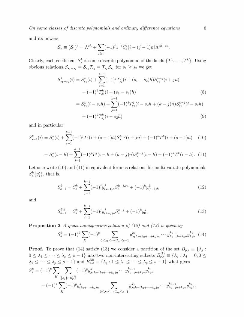
On some classes of discrete polynomials and ordinary difference equations 6
and its powers
Ss ≡ (S1)s = Λsh +
∑
j≥1
(−1)jz−jSjs(i− (j − 1)n)Λsh−jn.
Clearly, each coefficient Sks is some discrete polynomial of the fields {T 1, . . . , T k}. Using
obvious relations Ss1−s2 = Ss1Ts2 = Ts2Ss1 for s1 ≥ s2 we get
Sks1−s2
(i) = Sks1(i) +
k−1∑
j=1
(−1)jT js2(i+ (s1 − s2)h)S
k−js1
(i+ jn)
+ (−1)kT ks2(i+ (s1 − s2)h) (8)
= Sks1(i− s2h) +
k−1∑
j=1
(−1)jT js2(i− s2h+ (k − j)n)Sk−j
s1(i− s2h)
+ (−1)kT ks2(i− s2h) (9)
and in particular
Sks−1(i) = Sk
s (i) +
k−1∑
j=1
(−1)jT j(i+ (s− 1)h)Sk−js (i+ jn) + (−1)kT k(i+ (s− 1)h) (10)
= Sks (i− h) +
k−1∑
j=1
(−1)jT j(i− h+ (k − j)n)Sk−js (i− h) + (−1)kT k(i− h). (11)
Let us rewrite (10) and (11) in equivalent form as relations for multi-variate polynomials
Sks {y
rj}, that is,
Sks−1 = Sk
s +
k−1∑
j=1
(−1)jyj(s−1)hSk−j,jns + (−1)kyk(s−1)h (12)
and
Sk,hs−1 = Sk
s +
k−1∑
j=1
(−1)jyj(k−j)nSk−js + (−1)kyk0 . (13)
Proposition 2 A quasi-homogeneous solution of (12) and (13) is given by
Sks = (−1)k
∑
K
(−1)p∑
0≤λ1≤···≤λp≤s−1
yk1λ1h+(k2+···+kp)n
· · · ykp−1
λp−1h+kpnykpλph. (14)
Proof. To prove that (14) satisfy (13) we consider a partition of the set Bp,s ≡ {λj :
0 ≤ λ1 ≤ · · · ≤ λp ≤ s − 1} into two non-intersecting subsets B(1)p,s ≡ {λj : λ1 = 0; 0 ≤
λ2 ≤ · · · ≤ λp ≤ s− 1} and B(2)p,s ≡ {λj : 1 ≤ λ1 ≤ · · · ≤ λp ≤ s− 1} what gives
Sks = (−1)k
∑
K
∑
{λj}∈B(2)p,s
(−1)pyk1λ1h+(k2+···+kp)n
· · · ykp−1
λp−1h+kpnykpλph
+ (−1)k∑
K
(−1)pyk1(k2+···+kp)n
∑
0≤λ2≤···≤λp≤s−1
yk2λ2h+(k3+···+kp)n
· · · ykp−1
λp−1h+kpnykpλph.
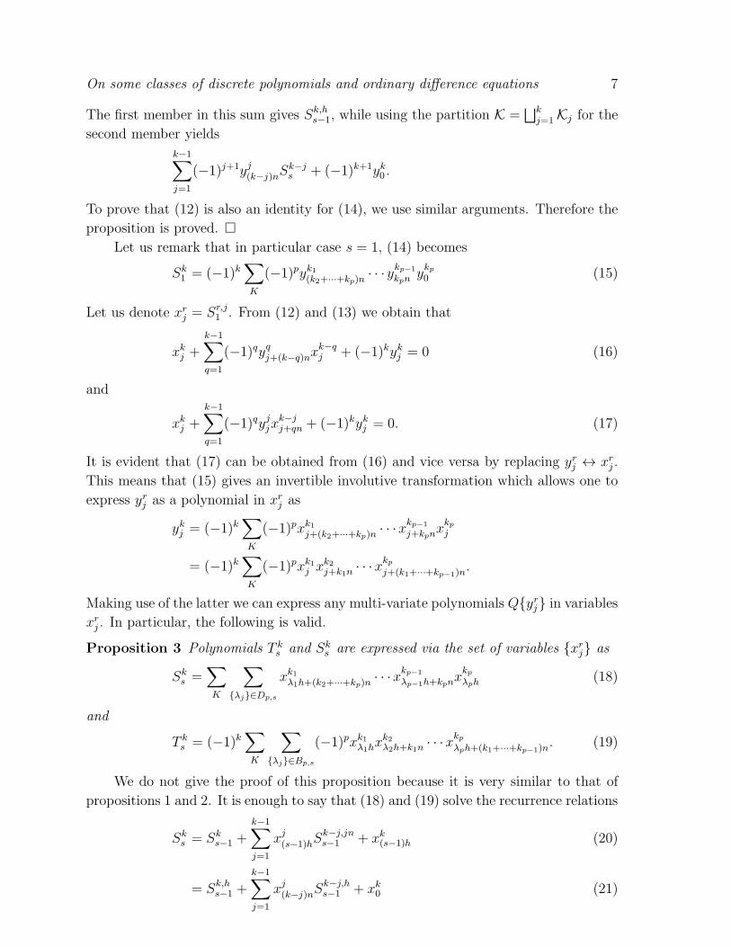
On some classes of discrete polynomials and ordinary difference equations 7
The first member in this sum gives Sk,hs−1, while using the partition K =
⊔k
j=1Kj for the
second member yields
k−1∑
j=1
(−1)j+1yj(k−j)nSk−js + (−1)k+1yk0 .
To prove that (12) is also an identity for (14), we use similar arguments. Therefore the
proposition is proved. �
Let us remark that in particular case s = 1, (14) becomes
Sk1 = (−1)k
∑
K
(−1)pyk1(k2+···+kp)n· · · y
kp−1
kpnykp0 (15)
Let us denote xrj = Sr,j1 . From (12) and (13) we obtain that
xkj +
k−1∑
q=1
(−1)qyqj+(k−q)nx
k−qj + (−1)kykj = 0 (16)
and
xkj +
k−1∑
q=1
(−1)qyjjxk−jj+qn + (−1)kykj = 0. (17)
It is evident that (17) can be obtained from (16) and vice versa by replacing yrj ↔ xrj .
This means that (15) gives an invertible involutive transformation which allows one to
express yrj as a polynomial in xrj as
ykj = (−1)k∑
K
(−1)pxk1j+(k2+···+kp)n
· · ·xkp−1
j+kpnxkpj
= (−1)k∑
K
(−1)pxk1j xk2j+k1n
· · ·xkp
j+(k1+···+kp−1)n.
Making use of the latter we can express any multi-variate polynomials Q{yrj} in variables
xrj . In particular, the following is valid.
Proposition 3 Polynomials T ks and Sk
s are expressed via the set of variables {xrj} as
Sks =
∑
K
∑
{λj}∈Dp,s
xk1λ1h+(k2+···+kp)n
· · ·xkp−1
λp−1h+kpnxkpλph
(18)
and
T ks = (−1)k
∑
K
∑
{λj}∈Bp,s
(−1)pxk1λ1hxk2λ2h+k1n
· · ·xkp
λph+(k1+···+kp−1)n. (19)
We do not give the proof of this proposition because it is very similar to that of
propositions 1 and 2. It is enough to say that (18) and (19) solve the recurrence relations
Sks = Sk
s−1 +
k−1∑
j=1
xj(s−1)hSk−j,jns−1 + xk(s−1)h (20)
= Sk,hs−1 +
k−1∑
j=1
xj(k−j)nSk−j,hs−1 + xk0 (21)
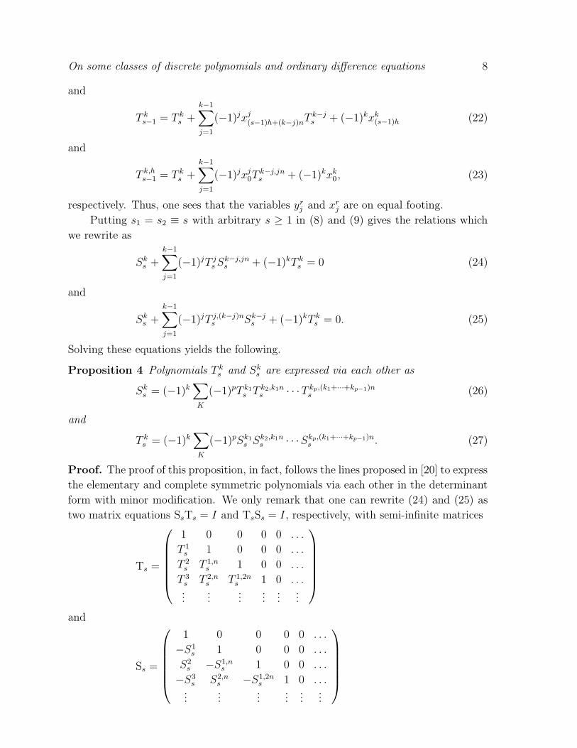
On some classes of discrete polynomials and ordinary difference equations 8
and
T ks−1 = T k
s +k−1∑
j=1
(−1)jxj(s−1)h+(k−j)nTk−js + (−1)kxk(s−1)h (22)
and
T k,hs−1 = T k
s +k−1∑
j=1
(−1)jxj0Tk−j,jns + (−1)kxk0, (23)
respectively. Thus, one sees that the variables yrj and xrj are on equal footing.
Putting s1 = s2 ≡ s with arbitrary s ≥ 1 in (8) and (9) gives the relations which
we rewrite as
Sks +
k−1∑
j=1
(−1)jT jsS
k−j,jns + (−1)kT k
s = 0 (24)
and
Sks +
k−1∑
j=1
(−1)jT j,(k−j)ns Sk−j
s + (−1)kT ks = 0. (25)
Solving these equations yields the following.
Proposition 4 Polynomials T ks and Sk
s are expressed via each other as
Sks = (−1)k
∑
K
(−1)pT k1s T k2,k1n
s · · ·T kp,(k1+···+kp−1)ns (26)
and
T ks = (−1)k
∑
K
(−1)pSk1s S
k2,k1ns · · ·Skp,(k1+···+kp−1)n
s . (27)
Proof. The proof of this proposition, in fact, follows the lines proposed in [20] to express
the elementary and complete symmetric polynomials via each other in the determinant
form with minor modification. We only remark that one can rewrite (24) and (25) as
two matrix equations SsTs = I and TsSs = I, respectively, with semi-infinite matrices
Ts =
1 0 0 0 0 . . .
T 1s 1 0 0 0 . . .
T 2s T 1,n
s 1 0 0 . . .
T 3s T 2,n
s T 1,2ns 1 0 . . .
......
......
......
and
Ss =
1 0 0 0 0 . . .
−S1s 1 0 0 0 . . .
S2s −S1,n
s 1 0 0 . . .
−S3s S2,n
s −S1,2ns 1 0 . . .
......
......
......

On some classes of discrete polynomials and ordinary difference equations 9
and I being semi-infinite identity matrix and use them the known expression for the
elements of an inverse matrix via the elements of the original one. As a result, in
particular, we obtain formulas (26) and (27), which can be presented in the determinant
form. �
2.2. Polynomials T js and Sj
s
Given an infinite number of constants cj, define
Ts ≡ Ts +∑
j≥1
z−jhcjTs+jn.
Observe that
Ts = Λ−sh +∑
j≥1
z−jT js (i− (j − 1)n− sh)Λ−sh−jn
with coefficients T js which can be described as follows. Let k = κh + r, where r stands
for the remainder of division of k by h, then
T ks (i) = T k
s (i) +κ∑
j=1
cjTk−jhs+jn (i).
Given an infinite number of constants Hj, define
Ss ≡ Ss +∑
j≥1
z−jhHjSs−jn.
Here it is supposed that s− jn ≤ 1. Observe that
Ss = Λsh +∑
j≥1
(−1)jz−jSjs(i− (j − 1)n)Λsh−jn
with
Sks (i) = Sk
s (i) +κ∑
j=1
(−1)jhHjSk−jhs−jn (i+ jhn).
It is evident that
Ts1+s2 = Ts1Ts2 = Ts2 Ts1, Ss1+s2 = Ss1Ss2 = Ss2Ss1 ,
Ts1−s2 = Ts1Ss2 = Ss2 Ts1 , Ss1−s2 = Ss1Ts2 = Ts2Ss1 .
This means, in particular, that polynomials T ks and Sk
s as well as polynomials T ks and
Sks also satisfy identities (3), (4), (10), (11), (20), (21), (22) and (23). The difference
between these solutions is that in the case of quasi-homogeneous polynomials T ks and
Sks one starts from T k
1 = T k and Sk1 given by (15), while for deriving polynomials T k
s
and Sks one uses as the initial data in the corresponding recurrence relations some linear
combinations of quasi-homogeneous polynomials.
On some classes of discrete polynomials and ordinary difference equations 10
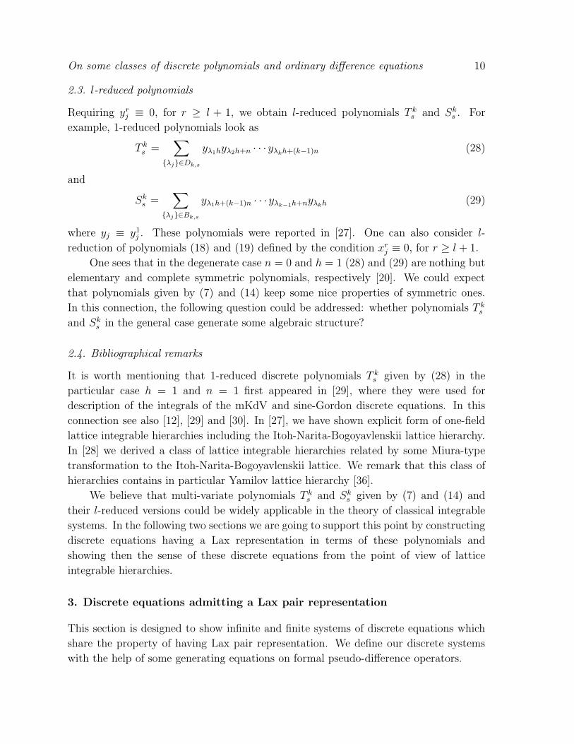
2.3. l-reduced polynomials
Requiring yrj ≡ 0, for r ≥ l + 1, we obtain l-reduced polynomials T ks and Sk
s . For
example, 1-reduced polynomials look as
T ks =
∑
{λj}∈Dk,s
yλ1hyλ2h+n · · · yλkh+(k−1)n (28)
and
Sks =
∑
{λj}∈Bk,s
yλ1h+(k−1)n · · · yλk−1h+nyλkh (29)
where yj ≡ y1j . These polynomials were reported in [27]. One can also consider l-
reduction of polynomials (18) and (19) defined by the condition xrj ≡ 0, for r ≥ l + 1.
One sees that in the degenerate case n = 0 and h = 1 (28) and (29) are nothing but
elementary and complete symmetric polynomials, respectively [20]. We could expect
that polynomials given by (7) and (14) keep some nice properties of symmetric ones.
In this connection, the following question could be addressed: whether polynomials T ks
and Sks in the general case generate some algebraic structure?
2.4. Bibliographical remarks
It is worth mentioning that 1-reduced discrete polynomials T ks given by (28) in the
particular case h = 1 and n = 1 first appeared in [29], where they were used for
description of the integrals of the mKdV and sine-Gordon discrete equations. In this
connection see also [12], [29] and [30]. In [27], we have shown explicit form of one-field
lattice integrable hierarchies including the Itoh-Narita-Bogoyavlenskii lattice hierarchy.
In [28] we derived a class of lattice integrable hierarchies related by some Miura-type
transformation to the Itoh-Narita-Bogoyavlenskii lattice. We remark that this class of
hierarchies contains in particular Yamilov lattice hierarchy [36].
We believe that multi-variate polynomials T ks and Sk
s given by (7) and (14) and
their l-reduced versions could be widely applicable in the theory of classical integrable
systems. In the following two sections we are going to support this point by constructing
discrete equations having a Lax representation in terms of these polynomials and
showing then the sense of these discrete equations from the point of view of lattice
integrable hierarchies.
3. Discrete equations admitting a Lax pair representation
This section is designed to show infinite and finite systems of discrete equations which
share the property of having Lax pair representation. We define our discrete systems
with the help of some generating equations on formal pseudo-difference operators.
On some classes of discrete polynomials and ordinary difference equations 11
3.1. The first class of discrete equations
Consider a partition Ts = (Ts)+,k + (Ts)−,k, where
(Ts)+,k ≡ Λ−sh +k∑
j=1
z−jT js (i− (j − 1)n− sh)Λ−sh−jn
and
(Ts)−,k ≡∑
j>k
z−jT js (i− (j − 1)n− sh)Λ−sh−jn.
Observe that
[(Ts)+,k, T1] =∑
j≥1
z−k−jνj(i)Λ−(s+1)h−(k+j)n,
where
νj(i) = T k+j(i− (s+ 1)h− (k + j − 1)n)
+k∑
q=1
T qs (i− sh− (q − 1)n)T k+j−q(i− (s+ 1)h− (k + j − 1)n)
− T k+j(i− h− (k + j − 1)n)
−k∑
q=1
T qs (i− (s+ 1)h− (k + j − 1)n)T k+j−q(i− h− (k + j − q − 1)n).
Let
(Ts)+,k = (Ts)+,k +∑
j≥1
z−jhcj(Ts+jn)+,k−jh.
As can be checked
(Ts)+,k = Λ−sh +
k∑
j=1
z−jT js (i− (j − 1)n− sh)Λ−sh−jn
and the commutativity equation
[(Ts)+,k, T1] = 0 (30)
generate an infinite number of discrete equations
T k+j(i+ sh) +
k∑
q=1
T qs (i)T
k+j−q(i+ sh+ qn)
= T k+j(i) +
k∑
q=1
T qs (i+ h+ (k + j − q)n)T k+j−q(i), j ≥ 1. (31)
Clearly, this system admits an l-reduction with the help of condition T j ≡ 0 for j ≥ l+1
yielding therefore an l-field system of ordinary difference equations.
On some classes of discrete polynomials and ordinary difference equations 12
Commutativity equation (30) appears as a condition of the compatibility of two
linear equations
(Ts)+,k(ψi) =w
zkψi, T1(ψi) = ψi
the first of which we can rewrite as
wψi+kn+sh = zkψi+kn +k∑
j=1
zk−jT js (i+ (k − j + 1)n)ψi+(k−j)n. (32)
Remark that w here is the second spectral parameter. The equation T1(ψi) = ψi with
l-reduced operator T1 looks as
zlψi+ln+h = zlψi+ln +l∑
j=1
zl−jT j(i+ (l − j + 1)n)ψi+(l−j)n. (33)
As a consequence of (30) we have
[(Ts)+,k,S1] = 0
which gives an infinite number of discrete equations
Sk+j(i+ sh) +
k∑
q=1
(−1)qT qs (i+ h)Sk+j−q(i+ sh+ qn)
= Sk+j(i) +
k∑
q=1
(−1)qT qs (i+ (k + j − q)n)Sk+j−q(i), j ≥ 1. (34)
This system also admits an l-reduction with the help of condition Sj ≡ 0 for j ≥ l + 1.
Linear problem S1(ψi) = ψi, in this case, becomes
zlψi+ln−h = zlψi+ln +
l∑
j=1
(−1)jzl−jSj(i+ (l − j + 1)n− h)ψi+(l−j)n. (35)
3.2. The second class of discrete equations
Consider a partition Ss = (Ss)+,k + (Ss)−,k, where
(Ss)+,k ≡ Λsh +
k∑
j=1
(−1)jz−jSjs(i− (j − 1)n)Λsh−jn
and
(Ss)−,k ≡∑
j>k
(−1)jz−jSjs(i− (j − 1)n)Λssh−jn.
Observe that
[(Ss)+,k, T1] =∑
j≥1
z−k−jµj(i)Λ(s−1)h−(k+j)n, (36)

On some classes of discrete polynomials and ordinary difference equations 13
with
µj(i) = T k+j(i+ (s− 1)h− (k + j − 1)n)
+
k∑
q=1
(−1)qSqs (i− (q − 1)n)T k+j−q(i+ (s− 1)h− (k + j − 1)n)
− T k+j(i− h− (k + j − 1)n)
−k∑
q=1
(−1)qSqs (i− h− (k + j − 1)n)T k+j−q(i− h− (k + j − q − 1)n).
Let
(Ss)+,k ≡ (Ss)+,k +∑
j≥1
z−jhHj(Ss−jn)+,k−jh
then
(Ss)+,k = Λsh +k∑
j=1
(−1)jz−jSjs(i− (j − 1)n)Λsh−jn.
We define the second class of discrete equations with the help of commutativity equation
[(Ss)+,k, T1] = 0, (37)
which yields an infinite number of discrete equations
T k+j(i+ sh) +
k∑
q=1
(−1)qSqs (i+ h + (k + j − q)n)T k+j−q(i+ sh)
= T k+j(i) +
k∑
q=1
(−1)qSqs (i)T
k+j−q(i+ qn), j ≥ 1. (38)
As a consequence of (37) we have Lax equation
[(Ss)+,k,S1] = 0, (39)
which gives
Sk+j(i+ sh) +
k∑
q=1
Sqs(i+ (k + j − q)n)Sk+j−q(i+ sh)
= Sk+j(i) +k∑
q=1
Sqs(i+ h)Sk+j−q(i+ qn), j ≥ 1. (40)
Clearly, commutativity equations (37) and (39) appear as a conditions of the
consistency of the linear equation
(Ss)+,k(ψi) =w
zkψi
which we can rewrite as
wψi−sh+kn = zkψi+kn+
k∑
j=1
(−1)jzk−jSjs(i−sh+(k− j+1)n)ψi+(k−j)n(41)
with T1(ψi) = ψi and S1(ψi) = ψi, respectively.
On some classes of discrete polynomials and ordinary difference equations 14
3.3. Remarks on Lax pairs
We have constructed infinite families of ordinary difference systems (31), (34), (38) and
(40), which are equivalent to the consistency conditions of the corresponding pairs of
linear equations. We suppose that Sks and T k
s are expressed via the set of the fields
{T j} in equations (31) and (38), while in (34) and (40) they are expressed via {Sj}.
Let us remember that these two sets of dynamical variables are related to each other
by involutive invertible transformation. In particular, we are interested in l-reduced
versions of these systems which are defined by condition T j ≡ 0, j ≥ l + 1 for (31)
and (38) and Sj ≡ 0, j ≥ l + 1 for (34) and (40). The first question which naturally
arise is: how do we construct the first integrals of the system under consideration using
corresponding pair of linear equations?
Consider a pair of the linear equations
ψi+N1 = L1(ψi, . . . , ψi+N1−1)
and
ψi+N2 = L2(ψi, . . . , ψi+N2−1),
for which the compatibility condition is equivalent to some system of ordinary difference
equations. For example, in the case (32) and (33), we have N1 = kn+sh andN2 = ln+h.
Choosing any of these equations, say the first one, we construct the vector-function
Ψ(i) = (ψ(0)(i), . . . , ψ(N1−1)(i))T , where ψ(j)(i) ≡ ψi+j . Then we use the rest equation
to construct linear equation L(i)Ψ(i) = 0 with some matrix-function L. The second
equation of the form Ψ(i+ 1) = A(i)Ψ(i) is easily defined by
ψ(j)(i+ 1) = ψ(j+1)(i), j = 1, . . . , N1 − 2
and
ψ(N1−1)(i+ 1) = L1(ψ(0)(i), . . . , ψ(N1−1)(i)).
Therefore the system under consideration are equivalent to the Lax equation
L(i+ 1)A(i) = A(i)L(i).
The condition detL = 0 gives us the spectral curve P (w, z) = 0.
3.4. Integrable hierarchies of lattice evolution equations
From (36) we see that
[(Ssn)+,sh, T1] =∑
j≥1
z−sh−jµj(i)Λ−h−jn.
This means that we can correctly define evolution equations by generating relation
∂sT1 = zsh[(Ssn)+,sh, T1] (42)
with
(Ssn)+,sh = Λshn +
sh∑
j=1
(−1)jz−jSjsn(i− (j − 1)n)Λshn−jn.
On some classes of discrete polynomials and ordinary difference equations 15
This generating equation gives an infinite number of evolution differential-difference
equations
∂sTj(i) = T sh+j(i) +
sh∑
q=1
(−1)qSqsn(i+ h+ (j − q)n)T sh+j−q(i)
− T sh+j(i− shn)−sh∑
q=1
(−1)qSqsn(i− shn)T sh+j−q(i− (sh− q)n). (43)
As a consequence of Lax equation (42) we have
∂sS1 = zsh[(Ssn)+,sh,S1]
which yields
∂sSj(i) = (−1)sh
{
Ssh+j(i) +sh∑
q=1
Sqsn(i+ (j − q)n)Ssh+j−q(i)
}
− (−1)sh
{
Ssh+j(i− shn)
+
sh∑
q=1
Sqsn(i− shn + h)Ssh+j−q(i− (sh− q)n)
}
. (44)
Observe that{
∂s +
s−1∑
q=1
Hq∂s−q
}
T1 = zsh[(Ssn)+,sh, T1].
From the latter we see that the stationarity equation{
∂s +
s−1∑
q=1
Hq∂s−q
}
T1 = 0
is equivalent to a special case of (37).
3.5. Some examples of lattice integrable hierarchies
Using (43) and (44), we are able to present the explicit form for a number of lattice
integrable hierarchies.
3.5.1. Itoh-Narita-Bogoyavlenskii lattice hierarchy Let h = 1 while n ≥ 1 is an
arbitrary integer. Lax equation (42) with the operator T1 = Λ−1 + z−1T (i − 1)Λ−1−n,
where T (i) ≡ T 1(i), gives evolution equations
∂sT (i) = (−1)sT (i) {Sssn(i− (s− 1)n+ 1)− Ss
sn(i− sn)} (45)
constituting an integrable hierarchy for the extended Volterra equation [21]
∂1T (i) = T (i)
{
n∑
j=1
T (i− j)−n∑
j=1
T (i+ j)
}
also known as the Itoh-Narita-Bogoyavlenskii lattice [16], [21], [6].
On some classes of discrete polynomials and ordinary difference equations 16
3.5.2. Bogoyavlenskii lattice hierarchy Now let n = 1 while h ≥ 1 is an arbitrary
integer. Lax equation (42) with the operator T1 = Λ−h + z−1Ti−hΛ−h−1 generates
integrable hierarchy
∂sT (i) = (−1)shT (i){
Sshs (i− (s− 1)h+ 1)− Ssh
s (i− sh)}
for the Bogoyavlenskii lattice
∂1T (i) = (−1)hT (i)
{
h∏
j=1
T (i+ j)−h∏
j=1
T (i− j)
}
.
3.5.3. Lattice Gel’fand-Dickii or (l + 1)-KdV hierarchy Let h = 1 and n = 1, while
l ≥ 1 be an arbitrary integer. With the operator
T1 = Λ−1 +
l∑
j=1
z−jT j(i− j)Λ−1−j
we obtain the evolution equations
∂sTj(i) = (−1)s+j
{
l∑
q=j
(−1)qSs+j−qs (i+ q − s+ 1)T q(i)
}
− (−1)s+j
{
l∑
q=j
(−1)qSs+j−qs (i− s)T q(i+ j − q)
}
for the lattice (l+1)-KdV hierarchy [1], [3], [4]. In the case l = 1, we obtain the Volterra
lattice hierarchy
∂sT (i) = (−1)sT (i) {Sss(i− s+ 2)− Ss
s(i− s)}
which, as is known, gives one of the lattice analogues of the KdV hierarchy. In the case
l = 2, we obtain the lattice Boussinesq hierarchy in the form
∂sT1(i) = (−1)s
{
Sss(i− s+ 2)T 1(i)− Ss−1
s (i− s+ 3)T 2(i)}
− (−1)s{
Sss(i− s)T 1(i)− Ss−1
s (i− s)T 2(i− 1)}
,
∂sT2(i) = (−1)sT 2(i) {Ss
s(i− s+ 3)− Sss(i− s)} .
whose the first flow is given by [3]
∂1T1(i) = T 2(i)− T 2(i− 1) + T 1(i)
{
T 1(i− 1)− T 1(i+ 1)}
,
∂1T2(i) = T 2(i)
{
T 1(i− 1)− T 1(i+ 2)}
.
3.6. Bibliographical remarks
We have not discussed above a quite important question concerning the Hamiltonian,
and what is more important from different points of view, the bi-Hamiltonian structure
of lattice integrable hierarchies with a finite and infinite number of fields given by (43)
and (44). In the previous subsection we have only presented some examples of lattice
integrable hierarchies known in the literature in their explicit form. One can find studies
on the Hamiltonian approach to lattice systems, for example, in [1], [3] - [5], [7], [9] and
[35].
On some classes of discrete polynomials and ordinary difference equations 17
4. Integrable hierarchies of lattice evolution equations from the point of
view of the KP hierarchy
In the previous section we have shown some classes of discrete equations with their Lax
representation in terms of polynomials T ks and Sk
s which were given in explicit form by
(7), (14), (18) and (19). In this section we have a look at that from another point of view.
In [23]-[27] we developed an approach which relates some evolutionary lattice equations
and their hierarchies to the KP hierarchy. We state in this section this approach. This
aims, in particular, to clarify the appearance of l-reduced versions of discrete equations
(31), (34), (38) and (40).
4.1. Free sequences of KP hierarchies. Invariant submanifolds
To begin with, we consider the free sequences of KP hierarchies {h(i, z) : i ∈ Z} in the
form of local conservation laws [11], [34], that is,
∂sh(i, z) = ∂H(s)(i, z), ∀i ∈ Z,
where the formal Laurent series h(z) = z+∑
j≥2 hjz−j+1 and H(s)(z) = zs+
∑
j≥1Hsj z
−j
are related to the KP wave function by h(z) = ∂ψ/ψ and H(s)(z) = ∂sψ/ψ, respectively.
Therefore, each coefficient Hsj is supposed to be some differential polynomial Hs
j =
Hsj [h2, . . . , hs+k]. More exactly, the Laurent series H(s)(z) is calculated as a projection
of zs on the linear space H+ =⟨
1, h, h(2), ...⟩
spanned by Faa di Bruno iterates
h(k) ≡ (∂ + h)k(1) . For example,
H(1) = h, H(2) = h(2) − 2h2, H(3) = h(3) − 3h2h− 3h3 − 3h′2
etc. Remark, that h(s)(z) = ∂sψ/ψ. As is known, dynamics of the coefficients of Hsj in
virtue of KP flows is defined by the invariance property(
∂s +H(s))
H+ ⊂ H+, ∀s ≥ 1. (46)
Conversely, it can be seen, that a hierarchy of dynamical systems governed by (46),
known as the Central System, is equivalent to the KP hierarchy [10]. Moreover, we
consider also a Laurent series a(i, z) = z+∑
j≥1 aj(i)z−j+1 ≡ zψi+1/ψi. By its definition,
it satisfies the following evolution equations
∂sa(i, z) = a(i, z){
H(s)(i+ 1, z)−H(s)(i, z)}
, (47)
which in turn can be presented in the form of differential-difference conservation laws
∂sξ(i, z) = H(s)(i+ 1, z)−H(s)(i, z)
with
ξ(i, z) = ln a(i) = ln z −∑
j≥1
1
j
(
−∑
k≥1
ak(i)z−k
)j
≡ ln z +∑
j≥1
ξj(i)z−j .
It is convenient to consider a free bi-infinite sequence of KP hierarchies as two equations
[19]
∂shk(i) = ∂Hsk−1(i), ∂sξk(i) = Hs
k(i+ 1)−Hsk(i). (48)
On some classes of discrete polynomials and ordinary difference equations 18
The two theorems given below yield an infinite number of invariant submanifolds
of the phase space of the sequence of KP hierarchies whose points are defined by
{ak(i), Hsk(i) : i ∈ Z}.
Theorem 1 [23] Submanifold Snk−1 defined by the condition
zk−na[n](i, z) ∈ H+(i), ∀i ∈ Z (49)
is invariant with respect to the flows given by evolution equations (48).
Here, by definition,
a[s](i, z) =
∏s
j=1 a(i+ j − 1, z), for s ≥ 1;
1, for s = 0;∏|s|
j=1 a−1(i− j, z), for s ≤ −1.
The condition (49) can be ultimately rewritten as a single generating relation∗
zk−na[n] = H(k) +
k∑
j=1
a[n]j H
(k−j), (50)
where a[s]j are defined as the coefficients of Laurent series a[s] = zs +
∑
j≥1 a[s]j z
s−j being
ultimately some quasi-homogeneous polynomials a[s]j = a
[s]j [a1, . . . , aj].
Theorem 2 [24] The following chain of inclusions
Sns−1 ⊂ S2n
2s−1 ⊂ S3n3s−1 ⊂ · · · (51)
is valid.
4.2. The nth discrete KP hierarchy
Let us consider the restriction of (48) on Sn0 which is defined by the condition
z1−na[n] = h+a[n]1 . Clearly, by this constraint we should get as a result some differential-
difference equations on infinite number of dynamical variables ak = ak(i) in the form
of differential-difference conservation laws, but there is a need to know how coefficients
Hsj are expressed via aj for all s ≥ 1. By our assumption, we already know that
H1k ≡ hk+1 = a
[n]k+1. To obtain explicit expressions for all Hs
k we must use theorem 2.
For s = 1, we have a chain
Sn0 ⊂ S2n
1 ⊂ S3n2 ⊂ · · ·
Solving, step-by-step, the defining equations for all invariant submanifolds in this chain
we come to [24]
Hsk = F
(n,s)k [a1, . . . , ak+s] ≡ a
[sn]k+s +
s−1∑
j=1
q(n,sn)j a
[(s−j)n]k+s−j . (52)
∗ Note that we sometimes do not indicate dependence on discrete variable i in formulas which contain
no shifts with respect to this variable.
On some classes of discrete polynomials and ordinary difference equations 19
Here q(n,r)j , being some quasi-homogeneous polynomials, are defined through the relation
zr = a[r] +∑
j≥1
q(n,r)j zj(n−1)a[r−jn]. (53)
We can code all relations (52) in one generating relation
H(s) = F (n,s) = zs−sn
{
a[sn] +
s∑
j=1
zj(n−1)q(n,sn)j a[(s−j)n]
}
, (54)
where F (n,s) ≡ zs +∑
j≥1 F(n,s)j z−j . Thus the restriction of dynamics given by (48) on
Sn0 yields evolution equations in the form of differential-difference conservation laws
∂sξk(i) = F(n,s)k (i+ 1)− F
(n,s)k (i) (55)
on an infinite number of fields {ak = ak(i)}. Let M be the corresponding phase space.
We call the hierarchy of the flows on M given by evolution equations (55) the nth
discrete KP hierarchy. Let us observe that in terms of KP wave function the relation
(54) takes the form
∂sψi = zsψi+sn +s∑
j=1
zs−jq(n,sn)j (i)ψi+(s−j)n, (56)
while (53) is equivalent to
zrψi = zrψi+r +∑
j≥1
zr−jq(n,r)j (i)ψi+r−jn.
As a condition of consistency of these linear equations we obtain the evolution equations
∂sq(n,r)k (i) = q
(n,r)k+s (i+ sn) +
s∑
j=1
q(n,sn)j (i)q
(n,r)k+s−j(i+ (s− j)n)−
− q(n,r)k+s (i)−
s∑
j=1
q(n,sn)j (i+ r − (k + s− j)n)q
(n,r)k+s−j(i) (57)
which, by their construction, are identities by virtue of the nth discrete KP hierarchy
(55).
4.3. Some identities for q(n,s)j and a
[s]j
Relation (53) yields the infinite triangle system
a[r]k +
k−1∑
j=1
a[r−jn]k−j q
(n,r)j + q
(n,r)k = 0, k ≥ 1 (58)
from which we can calculate, for example,
q(n,r)1 = −a[r]1 , q
(n,r)2 = −a[r]2 + a
[r]1 a
[r−n]1 ,
q(n,r)3 = −a[r]3 + a
[r]1 a
[r−n]2 + a
[r−2n]1 a
[r]2 − a
[r]1 a
[r−n]1 a
[r−2n]1
On some classes of discrete polynomials and ordinary difference equations 20
etc. It was shown in [27] that if (58) is valid then a more general identity
a[p]k (i) = a
[r]k (i) +
k−1∑
j=1
a[r−jn]k−j (i)q
(n,r−p)j (i+ p) + q
(n,r−p)k (i+ p), (59)
for all integers r and p, holds. Resolving the latter in favor of q(n,r−p)k (i+ p) yields
q(n,r−m)k (i+m) = a
[m]k (i) +
k−1∑
j=1
q(n,r−(k−j)n)j (i)a
[m]k−j(i) + q
(n,r)k (i).
We remark that polynomials a[s]j , by definition, must satisfy
a[s1+s2]k (i) = a
[s1]k (i) +
k−1∑
j=1
a[s1]j (i)a
[s2]k−j(i+ s1) + a
[s2]k (i+ s1)
= a[s2]k (i) +
k−1∑
j=1
a[s2]j (i)a
[s1]k−j(i+ s2) + a
[s1]k (i+ s2) (60)
while for q(n,s)j we have
q(n,s1+s2)k (i) = q
(n,s1)k (i) +
k−1∑
j=1
q(n,s1)j (i)q
(n,s2)k−j (i+ s1 − jn) + q
(n,s2)k (i+ s1)
= q(n,s2)k (i) +
k−1∑
j=1
q(n,s2)j (i)q
(n,s1)k−j (i+ s2 − jn) + q
(n,s1)k (i+ s2).
4.4. Restriction of the nth discrete KP hierarchy on submanifold Mn,p,l
To obtain in this framework the description of some integrable differential-difference
systems with a finite number of fields, we consider the intersection Sn0 ∩Sp
l−1. Obviously,
it is equivalent to the restriction of the flows of the nth discrete KP hierarchy on a
submanifold Mn,p,l ⊂ M. Taking into account (50) and (52), we immediately obtain
that defining equations for Mn,p,l are coded in the relation
zl−pa[p] = F (n,l) +l∑
j=1
a[p]j F
(n,l−j)
from which we derive
J(n,p,l)k [a1, . . . , ak+l] = 0, ∀k ≥ 1 (61)
with
J(n,p,l)k = a
[p]k+l − F
(n,l)k −
l−1∑
j=1
a[p]j F
(n,l−j)k
= a[p]k+l(i)− a
[ln]k+l(i)−
l−1∑
j=1
q(n,ln−p)j (i+ p)a
[(l−j)n]k+l−j (i). (62)
On some classes of discrete polynomials and ordinary difference equations 21
We see from (62) that J(n,ln,l)k = 0 is just an identity and, therefore, produces no invariant
submanifold. This is because Sn0 ⊂ S ln
l−1 by virtue of theorem 2.
Let us observe that, taking into account (59), we can rewrite (62) as
J(n,p,l)k = Q
(n,p,l)k +
k−1∑
j=1
a[−(k−j)n]j Q
(n,p,l)k−j , (63)
where Q(n,p,l)k (i) ≡ q
(n,ln−p)k+l (i+ p). Resolving this quasi-linear infinite triangle system in
favor of Q(n,p,l)k gives
Q(n,p,l)k = J
(n,p,l)k +
k−1∑
j=1
q(n,−(k−j)n)j J
(n,p,l)k−j (64)
for all k ≥ 1. This means that, in principle, we can define the submanifold Mn,p,l by
equations Q(n,p,l)k [a1, . . . , ak+l] = 0.
4.5. Linear equations on KP wave function corresponding to submanifold Mn,p,l
Some remarks about linear equations on the KP formal wave function ψi which follows
as a result of the restriction of the nth discrete KP hierarchy on the submanifold Mn,p,l
are in order. Let J (n,p,l)(z) ≡∑
j≥1 J(n,p,l)j z−j . We observe that an infinite number of
equations (61) can be presented by single a generating relation
J (n,p,l)(i, z) = zl−pa[p](i, z)
−zl−ln
{
a[ln](i, z) +l∑
j=1
zj(n−1)q(n,ln−p)j (i+ p)a[(l−j)n](i, z)
}
= 0.
Clearly, in terms of KP wave function, we can rewrite the latter relation as
J (n,p,l)(i, z) =zlψi+p − zlψi+ln −
∑l
j=1 zl−jq
(n,ln−p)j (i+ p)ψi+(l−j)n
ψi
= 0.
Thus in terms of the KP wave function the restriction of nth discrete KP hierarchy on
Mn,p,l is given by the linear equation
zlψi+ln +
l∑
j=1
zl−jq(n,ln−p)j (i+ p)ψi+(l−j)n = zlψi+p. (65)
Second linear equation which we should have in mind is (56).
What we obtain is that on Mn,p,l the KP wave function satisfies a linear equation
T1(ψi) = ψi with the l-reduced operator T1 in the case ln− p ≤ −1 while if ln− p ≥ 1
then it satisfies the equation S1(ψi) = ψi with l-reduced operator S1. So, let
h =
{
p− ln if ln− p ≤ −1;
ln− p if ln− p ≥ 1.
Let us denote
q(n,ln−p)j (i) = T j(i− h− (j − 1)n), j = 1, . . . , l
On some classes of discrete polynomials and ordinary difference equations 22
in the first case and
q(n,ln−p)j (i) = (−1)jSj(i− (j − 1)n), j = 1, . . . , l
in the second case, respectively. Substituting the latter into (65) gives (33) and (35).
We observe that in both cases
q(n,−sh)j (i) = T j
s (i− sh− (j − 1)n) (66)
and
q(n,sh)j (i) = (−1)jSj
s(i− (j − 1)n). (67)
Let us turn now to equation (56) defining an infinite number of flows of the nth
discrete KP hierarchy and consider only the flows ∂sh. With (67) we obtain
∂shψi = zshψi+shn +
sh∑
j=1
zsh−jq(n,shn)j (i)ψi+(sh−j)n
= zsh
{
ψi+shn +
sh∑
j=1
(−1)jz−jSjsn(i− (j − 1))ψi+(sh−j)n
}
= zsh (Ssn)+,sh (ψi). (68)
Let us summarize what we have said above. Restricting the nth discrete KP
hierarchy to Mn,p,l or more exactly its sub-hierarchy {∂sh : s ≥ 1}, where h is defined by
the triple (n, p, l) as above, leads to l-reduced lattice systems (43) or (44) in dependence
of the sign of ln − p. In the following two subsections we show how discrete equations
(31), (34), (38) and (40) appear in this framework and therefore we clarify their meaning.
4.6. Weaker invariance conditions
We have shown above that some integrable lattices can be obtained by imposig some
suitable conditions compatible with the flows of the nth discrete KP hierarchy on Mn,p,l
and presented some examples known in the literature. In this section, we are going to
show that there exist weaker invariance conditions. To this aim, we observe that the
relations
∂sQ(n,p,l)k (i) = Q
(n,p,l)s+k (i+ sn) +
s∑
j=1
q(n,sn)j (i+ p)Q
(n,p,l)s+k−j(i+ (s− j)n)
−Q(n,p,l)s+k (i)−
s∑
j=1
q(n,sn)j (i− (s+ k − j)n)Q
(n,p,l)s+k−j(i) (69)
are valid by virtue of the nth discrete KP hierarchy. Let {I(n,p,l)k : k ≥ 1} be some infinite
set of quasi-homogeneous polynomials related with {Q(n,p,l)k : k ≥ 1} by relations
Q(n,p,l)k = I
(n,p,l)k +
k−1∑
j=1
ξk−1,jI(n,p,l)k−j (70)
On some classes of discrete polynomials and ordinary difference equations 23
with some unknown coefficients ξk,s to be defined . Consider equation (69) on Q(n,p,l)1 =
I(n,p,l)1 , that is,
∂sQ(n,p,l)1 (i) = Q
(n,p,l)s+1 (i+ sn) +
s∑
j=1
q(n,sn)j (i+ p)Q
(n,p,l)s+1−j(i+ (s− j)n)
−Q(n,p,l)s+1 (i)−
s∑
j=1
q(n,sn)j (i− (s+ 1− j)n)Q
(n,p,l)s+1−j(i). (71)
Substituting (70) into the right-hand side of (71) gives
∂sI(n,p,l)1 (i) = I
(n,p,l)s+1 (i+ sn) +
s∑
j=1
ξs,j(i+ sn)I(n,p,l)s−j+1(i+ sn) + q
(n,sn)1 (i+ p)
×
{
I(n,p,l)s (i+ (s− 1)n) +s−1∑
j=1
ξs−1,j(i+ (s− 1)n)I(n,p,l)s−j (i+ (s− 1)n)
}
+ · · ·
+ q(n,sn)s (i+ p)I(n,p,l)1 (i)− I
(n,p,l)s+1 (i)−
s∑
j=1
ξs,j(i)I(n,p,l)s−j+1(i)− q
(n,sn)1 (i− sn)
×
{
I(n,p,l)s (i) +
s−1∑
j=1
ξs−1,j(i)I(n,p,l)s−j (i)
}
− · · · − q(n,sn)s (i− n)I(n,p,l)1 (i).
Impose now the periodicity condition Ik(i+n) = Ik(i) for all k ≥ 1. With this condition
∂sI(n,p,l)1 (i) =
{
ξs,1(i+ sn) + q(n,sn)1 (i+ p)− ξs,1(i)− q
(n,sn)1 (i− sn)
}
I(n,p,l)s (i)
+{
ξs,2(i+ sn) + q(n,sn)1 (i+ p)ξs−1,1(i+ (s− 1)n) + q
(n,sn)2 (i+ p)
−ξs,2(i)− q(n,sn)1 (i− sn)ξs−1,1(i)− q
(n,sn)2 (i− (s− 1)n)
}
I(n,p,l)s−1 (i) + · · ·
+
{
ξs,s(i+ sn) +
s−1∑
j=1
q(n,sn)j (i+ p)ξs−j,s−j(i+ (s− j)n) + q(n,sn)s (i+ p)
−ξs,s(i)−s−1∑
j=1
q(n,sn)j (i− (s− j + 1)n)ξs−j,s−j(i)− q(n,sn)s (i− n)
}
I(n,p,l)1 (i).
Now we observe that if ξs,k(i) = q(n,−p−(s−k+1)n)k (i+ p), then the coefficients at I
(n,p,l)j in
the last relation become identically zeros. So, let
Q(n,p,l)k (i) = I
(n,p,l)k (i) +
k−1∑
j=1
q(n,−p−(k−j)n)j (i+ p)I
(n,p,l)k−j (i). (72)
One can check that resolving these relations in favor of I(n,p,l)k yields
I(n,p,l)k (i) = Q
(n,p,l)k (i) +
k−1∑
j=1
a[−p−(k−j)n]j (i+ p)Q
(n,p,l)k−j (i). (73)
Taking into account (64), we derive from (73)
I(n,p,l)k (i) = J
(n,p,l)k (i) +
k−1∑
j=1
a[−p]j (i+ p)J
(n,p,l)k−j (i) (74)
On some classes of discrete polynomials and ordinary difference equations 24
and
J(n,p,l)k = I
(n,p,l)k +
k−1∑
j=1
a[p]j (i)I
(n,p,l)k−j .
In terms of the Laurent series relations, (74) takes the form
I(n,p,l)(i, z) = zpa[−p](i+ p, z)J (n,p,l)(i, z)
=ψi
ψi+p
J (n,p,l)(i, z)
=zlψi+p − zlψi+ln −
∑l
j=1 zl−jq
(n,ln−p)j (i+ p)ψi+(l−j)n
ψi+p
.
Therefore, we have proved the following. If all I(n,p,l)k defined by (73) satisfy the
periodicity condition
I(n,p,l)k (i+ n) = I
(n,p,l)k (i) (75)
then I(n,p,l)1 do not depend of all evolution parameters ts. Using similar reasoning,
step-by-step, we can show that under this condition in fact all I(n,p,l)k for k ≥ 1 are
constants. It is evident that by virtue of (72), the equations I(n,p,l)k ≡ 0 define the
invariant submanifold Mn,p,l while the periodicity condition (75) is weaker than the
latter condition. We observe that the coefficients of equations (69) considered as quasi-
linear equations with respect to Q(n,p,l)k do not depend on l. This means that periodicity
conditions I(n,p,l)k (i+ n) = I
(n,p,l)k (i) where
I(n,p,l)k ≡ I
(n,p,l)k +
l∑
j=1
hjI(n,p,l−j)k (76)
with arbitrary constants hj also select some invariant submanifold. Let d be some divisor
of the number n, then, it is obvious that the periodicity conditions
I(n,p,l)k (i+ d) = I
(n,p,l)k (i) (77)
define some invariant submanifold N dn,p,l of the nth discrete KP hierarchy. Let us
formulate all the above-mentioned in the following theorem.
Theorem 3 Infinite number of the periodicity conditions (77), where polynomials I(n,p,l)k
are defined by (73) and (76) and d is some divisor of n, are compatible with the flows
of the nth discrete KP hierarchy.
4.7. Discrete equations (31), (34), (38) and (40) as reductions of evolution
differential-difference equations
Here, we use the quite general theorem 3 to construct classes of constraints compatible
with integrable hierarchies corresponding to different submanifolds Mn,p,l . Let the
On some classes of discrete polynomials and ordinary difference equations 25
triple of integers (n, p, k) be such that kn − p = sh for some arbitrary s ≥ 0, then by
virtue of (67)
I(n,p,k)(i, z) =zkψi+p − zkψi+kn −
∑k
j=1 zk−jq
(n,kn−p)j (i+ p)ψi+(k−j)n
ψi+p
=zkψi+p − zkψi+kn −
∑k
j=1(−1)jzk−jSjs(i+ p− (j − 1)n)ψi+(k−j)n
ψi+p
.
Replacing k 7→ k − qh, s 7→ s− qn and therefore p 7→ p, we obtain
I(n,p,k−qh)(i, z) =
{
zk−qhψi+p − zk−qhψi+(k−qh)n
−
k−qh∑
j=1
(−1)jzk−qh−jSjs−qn(i+ p− (j − 1)n)ψi+(k−qh−j)n
}
/ψi+p
and consequently
I(n,p,k)(i, z) ≡ I(n,p,k)(i, z) +κ∑
q=1
HqI(n,p,k−qh)(i, z)
=
{(
zk +κ∑
q=1
Hqzk−qh
)
ψi+p
−zkψi+kn −k∑
j=1
(−1)jzk−jSjs(i+ p− (j − 1)n)ψi+(k−j)n
}
/ψi+p. (78)
Impose the condition
I(n,p,k)(i, z) =∑
j≥1
Ijz−j ,
where Ij’s are some constants. According to theorem 3 this condition is invariant with
respect to the flows of the nth discrete KP hierarchy. One sees that (78) becomes linear
problem (41), with
w = zk +
κ∑
q=1
Hqzk−qh −
∑
j≥1
Ijz−j .
By analogy, let the triple of integers (n, p, k) be such that kn− p = −sh for some
arbitrary s ≥ 0. Then by virtue of (66)
I(n,p,k)(i, z) =zkψi+p − zkψi+kn −
∑k
j=1 zk−jq
(n,kn−p)j (i+ p)ψi+(k−j)n
ψi+p
=zkψi+p − zkψi+kn −
∑k
j=1 zk−jT j
s (i+ (k − j + 1)n)ψi+(k−j)n
ψi+p
.
Imposing invariant condition
I(n,p,k)(i, z) ≡ I(n,p,k)(i, z) +κ∑
q=1
cqI(n,p,k−qh)(i, z) =
∑
j≥1
Ijz−j
leads to linear problem (32).
On some classes of discrete polynomials and ordinary difference equations 26
4.8. Examples
4.8.1. One-field difference systems In the case Mn,n+1,1 we have ln − p = −1 and
therefore h = p−ln = 1. In this situation the nth discrete KP hierarchy is reduced to the
Itoh-Narita-Bogoyavlenskii lattice given by (45). Two classes of compatible constraints
are deduced as the one-field reduction of discrete equations (31) and (38), that is,
T ks (i)T (i+ s+ kn) = T k
s (i+ n+ 1)T (i)
and
Sks (i)T (i+ kn) = Sk
s (i+ n+ 1)T (i+ s),
respectively, with
T ks (i) = T k
s (i) +
k∑
j=1
cjTk−js+jn(i)
and
Sks (i) = Sk
s (i) +k∑
j=1
(−1)jHjSk−js−jn(i+ jn).
Remember that we suppose here that s − jn ≤ 1. A more general class of one-field
lattices is given by
T ks (i)T (i+ sh + kn) = T k
s (i+ n+ h)T (i) (79)
and
Sks (i)T (i+ kn) = Sk
s (i+ n+ h)T (i+ sh), (80)
where h and n are supposed to be co-prime positive integers. Both the equations
(80) and (79) are of the form of the autonomous difference equation (1) with the
order N = sh + kn whose right-hand side is a rational function of its arguments
and corresponding parameters. Let us observe that making use of the identities for
polynomials T ks and Sk
s we can rewrite discrete equations (80) and (79) in the following
equivalent form:
T ks−1(i+ h)T (i+ sh + kn) = T k
s−1(i+ n+ h)T (i) (81)
and
Sks+1(i)T (i+ kn) = Sk
s+1(i+ n)T (i+ sh). (82)
It is evident from this that in the case n = 0 and h = 1 which corresponds to symmetric
multi-variate polynomials T ks {yj} and Sk
s {yj}, equations (82) and (81) are specified only
as the periodicity equation T (i+ s) = T (i).
On some classes of discrete polynomials and ordinary difference equations 27
4.8.2. The case h = n = 1 The simplest case, when we can obtain nontrivial discrete
nonlinear equations different from the periodicity one is h = n = 1. In this case (82)
and (81) looks as
T ks−1(i+ 1)T (i+ s+ k) = T k
s−1(i+ 2)T (i) (83)
and
Sks+1(i)T (i+ k) = Sk
s+1(i+ 1)T (i+ s). (84)
What we know is that these equations play the role of compatible constraints for
the Volterra lattice hierarchy defining invariant submanifolds in solution space of the
Volterra lattice. We claim but do not prove here that for an arbitrary fixed pair (k, s)
such that s ≥ k + 1, (84) and (83) represents in fact the same dynamical system. The
point is that one can transform (84) into (83) and back by interchanging {c1, . . . , ck}
and {H1, . . . , Hk} (cf. [22]). We will prove this fact in a subsequent publication.
For spectral curves, our calculations using Lax operators defined by (32) and (33),
in the case h = n = l = 1, yield the following. If s+ k = 2g + 1, where g ≥ k we obtain
H0w2 + zg+1Rg(z)w − z2g+1Rk(z) = 0, (85)
while in the case s+ k = 2g + 2 , where g ≥ k, we get
H0w2 − zg+1Rg+1(z)w + z2g+2Rk(z) = 0, (86)
with Rg(z) = zg +∑g
j=1Hjzg−j and Rk(z) = zk +
∑k
j=1 Hjzk−j, where Hj =
Hj +∑j−1
q=1 cqHj−q + cj. We remark that Hj’s are the first integrals integrals of equation
(83), while cj’s are the parameters entered in these equations. In particular,
H0 =
∏s+k
j=1 Ti+j−1
T ks−1(i+ 1)
. (87)
In both cases we have an expansion
w = zk +k∑
j=1
cjzk−j −
∑
j≥1
Ijz−j ,
where the coefficients Ij are some polynomials of variables Hj and cj.
Let us remark that in both cases we have a hyperelliptic spectral curve of genius g.
For (85), with the help of birational transformation
z =1
Z, w =
W − rg(Z)
2H0Z2g+1, W =
2H0w + zg+1Rg(z)
2z2g+1,
where
rg(Z) ≡ ZgRg
(
1
Z
)
, rk(Z) ≡ ZkRk
(
1
Z
)
,
we get
W 2 = P2g+1(Z) ≡ r2g(Z) + 4H0Z2g−k+1rk(Z),
On some classes of discrete polynomials and ordinary difference equations 28
while for (86), we use
z = Z, w = Zg+1W +Rg+1(Z)
2H0, W =
2H0w − zg+1Rg+1(z)
zg+1
to obtain
W 2 = P2g+2(Z) ≡ R2g+1(Z)− 4H0Rk(Z).
Making use of the transformation
w 7→zg+1
H0
(
zg−kw − Rg(z))
for (85) gives
z2g−2k+1w2 − zg−k+1Rg(z)w −H0Rk(z) = 0 (88)
while the transformation
w 7→zg+1
H0
(
Rg+1(z)− zg−k+1w)
converts (86) to the following form:
z2g−2k+2w2 − zg−k+1Rg+1(z)w +H0Rk(z) = 0. (89)
The reason why we have shown these transformations is that (88) and (89) are nothing
but the spectral curves for Lax operators defined by (33) and (41), in the case
h = n = l = 1. Let us remark that in this case {H1, . . . , Hk} is the set of the parameters
entered in equation (84), while other Hj’s and all cj’s are the first integrals. We will
describe in full detail all these integrals in a subsequent publication.
4.9. Bibliographical remarks
Let us remark that (84) has obvious integral♯
H0 = (−1)kSks+1(i)
s−1∏
j=k
T (i+ j). (90)
In particular case k = 1 one has
H0 = −{
S1s+1(i)−H1
}
s−1∏
j=1
T (i+ j),
where S1s+1(i) =
∑s
j=0 T (i+ j). The latter equation restricted by the condition H1 = 0
together with its integrals can be found in [12] (eq. (4)). In particular, in that paper
plausible formula was found yielding degrees of mapping iterates suggesting that this
equation has zero algebraic entropy.
♯ Here we use the same symbol H0 as in (87) because as we have already said equations (84) and (83)
for fixed pair (k, s) represent the same dynamical system. Therefore the integral H0 has two different,
at first glance, forms (87) and (90).
On some classes of discrete polynomials and ordinary difference equations 29
5. Discussion
Studies carried out in [12], [17], [27], [28], [29] and in this paper suggest that the
polynomials T ks and Sk
s corresponding to different pairs of co-prime integers n and h
might be quite universal and convenient combinatorial object and therefore we hope
that they deserve attention to investigate them.
Unfortunately, in this paper we have not considered in full detail the important
question of the structure of the first integrals for the obtained ordinary difference
equations and corresponding spectral curves P (w, z) = 0. We hope to fill this gap
in the following publications to investigate one-field equations (80) and (79) and, in
particular, equations (84) and (83). Also, we would like to study the relationship of the
explicit form of integrable hierarchies (43) and (44) with their Hamiltonian structures.
Acknowledgments
I wish to thank the referees for carefully reading the manuscript and for remarks which
enabled the presentation of the paper to be improved. This work was partially supported
by grant NSh-5007.2014.9.
References
[1] Antonov A, Belov A A and Chaltikian K D 1993 Lattice conformal theories and their integrable
perturbations J. Geom. Phys. 22 298-318
[2] Bellon M P and Viallet C-M Algebraic entropy 1999 Commun. Math. Phys. 204 425-37
[3] Belov A A and Chaltikian K D 1993 Lattice analogues of W -algebras and classical integrable
equations Phys. Lett. B 309 268-74
[4] Belov A A and Chaltikian K D 1993 Lattice analogue of the W -infinity algebra and discrete
KP-hierarchy Phys. Lett. B 317 64-72
[5] B laszak M and Marciniak K 1994 R-matrix approach to lattice integrable systems J. Math. Phys.
35 4661-82
[6] Bogoyavlensky O I 1988 Integrable discretizations of the KdV equation Phys. Lett. A 134 34-8
Bogoyavlenskii O I 1991 Algebraic constructions of integrable dynamical systems — extensions
of the Volterra system Russian Math. Surveys 46 1-46
[7] Bonora L and Xiong C S 1993 Multi-matrix models without continuum limit Nucl. Phys. B 405
228-75
[8] Bruschi M, Ragnisco O, Santini P M, and Zhang T G 1991 Integrable simplectic maps Physica D
49 273-94
[9] Carlet G 2006 The extended bigraded Toda hierarchy J. Phys. A: Math. Gen. 39 9411-35
[10] Casati P, Falqui G, Magri F and Pedroni M 1996 The KP theory revisited I, II, III, IV SISSA
preprints, ref. SISSA/2-5/96/
[11] Cherednik I 1978 Differential equations for the Baker-Akhiezer functions of algebraic curves Funct.
Anal. Appl. 12 195-203
[12] Demskoi D K, Tran D T, van der Kamp P H and Quispel G R W 2012 A novel nth order difference
equation that may be integrable J. Phys. A: Math. Theor 45 (Art. No. 135202) 10 pp.
[13] Grammaticos B, Ramani A and Papageorgiou V Do integrable mappings have the Painleve
property? 1991 Phys. Rev. Lett. 67 1825-8
On some classes of discrete polynomials and ordinary difference equations 30
[14] Hietarinta J and Viallet C 1998 Singularity confinement and chaos in discrete systems Phys. Rev.
Lett. 81 325-8
[15] Hone A N W, van der Kamp P H, Quispel G R W, and Tran D T 2013 Integrability of reductions
of the discrete Kortewegde Vries and potential Kortewegde Vries equations Proc. R. Soc. A 469
(Art. No. 20120747).
[16] Itoh Y 1975 An H-theorem for a system of competing species Proc. Japan Acad. 51 374-9
[17] van der Kamp P H, Rojas O and Quispel G R W 2007 Closed-form expressions for integrals of
MKdV and sine-Gordon maps J. Phys. A: Math. Theor. 40 12789-98
[18] van der Kamp P H, and Quispel G R W 2010 The staircase method: integrals for periodic
reductions of integrable lattice equations J. Phys. A: Math. Theor. 43 (Art. No. 465207) 34
pp.
[19] Magri F, Pedroni M and Zubelli J P 1997 On the geometry of Darboux transformations for the KP
hierarchy and its connection with the discrete KP hierarchy Commun. Math. Phys. 188 305-25
[20] Makdonald I G Symmetric functions and Hall polynomials, Second Edition, Oxford University
Press, 1995.
[21] Narita K 1982 Soliton solutions to extended Volterra equation J. Phys. Soc. Japan 51 1682-5
[22] Roberts J A G, Iatrou A, Quispel G R W 2002 Interchanging parameters and integrals in dynamical
systems: the mapping case J. Phys. A: Math. Gen. 35 2309-25
[23] Svinin A K 2002 Extended discrete KP hierarchy and its reductions from a geometric viewpoint
Lett. Math. Phys. 61 231-39
[24] Svinin A K 2004 Invariant submanifolds of the Darboux-Kadomtsev-Petviashvili chain and an
extension of the discrete Kadomtsev-Petviashvili hierarchy Theor. Math. Phys. 141 1542-61
[25] Svinin A K 2008 Reductions of integrable lattices J. Phys. A: Math. Theor. 41 (Art. No. 315205)
15 pp.
[26] Svinin A K 2009 On some class of reductions for the Itoh-Narita-Bogoyavlenskii lattice J. Phys.
A: Math. Theor. 41 (Art. No. 454021) 15 pp.
[27] Svinin A K 2011 On some class of homogeneous polynomials and explicit form of integrable
hierarchies of differential-difference equations J. Phys. A: Math. Theor. 44 (Art. No. 165206) 16
pp.
[28] Svinin A K 2011 On some integrable lattice related by Miura-type transformation to the Itoh-
Narita-Bogoyavlenskii lattice J. Phys. A: Math. Theor. 44 (Art. No. 465210) 8 pp.
[29] Tran D T, van der Kamp P H and Quispel G R W 2009 Closed-form expressions for integrals of
traveling wave reductions of integrable lattice equations J. Phys. A: Math. Theor. 42 (Art. No.
225201) 20 pp.
[30] Tran D T, van der Kamp P H and Quispel G R W 2010 Sufficient number of integrals for the
pth-order Lyness equation J. Phys. A: Math. Theor. 43 (Art. No. 302001) 11 pp.
[31] Tran D T, van der Kamp P H and Quispel G R W 2011 Involutivity of integrals of sine-Gordon,
modifieg KdV, and potential KdV maps J. Phys. A: Math. Theor. 44 (Art. No. 295206) 13 pp.
[32] Veselov A P 1991 Integrable maps Russ. Math. Surv. 46 1-51
[33] Veselov A P 1992 Growth and integrability in the dynamics of mappings Commun. Math. Phys.
145 181-93
[34] Wilson G 1981 On two constructions of conservation laws for Lax equations Quart. J. Math. Oxford
32 491–512
[35] Xiong C S 1992 Generalized integrable lattice systems Phys. Lett. B 279 341-6
[36] Yamilov R I 1983 Classification of discrete evolution equations Usp. Mat. Nauk 38 155–6 (in
Russian)