on some hereditary properties of riemannian -natural ...nice examples and counterexamples of several...

ah,

an 1

kith.metrical

rno),t

slar

Differential Geometry and its Applications 22 (2005) 19–47www.elsevier.com/locate/difgeo

On some hereditary properties of Riemanniang-natural metricson tangent bundles of Riemannian manifolds

Mohamed Tahar Kadaoui Abbassia,∗, Maâti Sarihb

a Département des Mathématiques, Faculté des sciences Dhar El Mahraz, Université Sidi Mohamed Ben AbdallB.P. 1796, Fès-Atlas, Fès, Morocco

b Département des Mathématiques et Informatique, Faculté des sciences et techniques de Settat, Université Hasser,B.P. 577, 26000 Morocco

Received 16 July 2003; received in revised form 19 October 2003

Available online 8 September 2004

Communicated by O. Kowalski

Abstract

It is well known that if the tangent bundleTM of a Riemannian manifold(M,g) is endowed with the Sasametricgs , then the flatness property onTM is inherited by the base manifold [Kowalski, J. Reine Angew. Ma250 (1971) 124–129]. This motivates us to the general question if the flatness and also other simple geoproperties remain “hereditary” if we replacegs by the most general Riemannian “g-natural metric” onTM (see[Kowalski and Sekizawa, Bull. Tokyo Gakugei Univ. (4) 40 (1988) 1–29; Abbassi and Sarih, Arch. Math. (Bsubmitted for publication]). In this direction, we prove that if(TM,G) is flat, or locally symmetric, or of constansectional curvature, or of constant scalar curvature, or an Einstein manifold, respectively, then(M,g) possessethe same property, respectively. We also give explicit examples ofg-natural metrics of arbitrary constant scacurvature onTM. 2004 Elsevier B.V. All rights reserved.

MSC:primary 53B20, 53C07; secondary 53A55, 53C25

Keywords:Riemannian manifold; Tangent bundle; Natural operation;g-natural metric;F -tensor field; Curvatures

* Corresponding author.E-mail address:[email protected](M.T.K. Abbassi).

0926-2245/$ – see front matter 2004 Elsevier B.V. All rights reserved.doi:10.1016/j.difgeo.2004.07.003

http://www.elsevier.com/locate/difgeo

mailto:[email protected]

20 M.T.K. Abbassi, M. Sarih / Differential Geometry and its Applications 22 (2005) 19–47

alf such

presentseme

et

we

urva-

n

Introduction and main results

If (M,g) is anm-dimensional Riemannian manifold, then the Sasaki metricgs is the most ‘natural’metric on its tangent bundleTM depending only on the Riemannian structure onM . Other metrics onTM, naturally constructed from the base metricg, are given in[11]. Indeed, using the concept of “naturoperations” and related notions, O. Kowalski and M. Sekizawa have given a full classification ometrics, supposing thatM is oriented. Other presentations of the basic results from[11] (involving alsothe non-oriented case and something more) can be found in[9] or [12] (see also[1]). We have studiedthese metrics in[3] and[4] and we have called themg-natural metrics on TM.

The Sasaki metric has been extensively studied, but it has been shown in many papers that ita kind of rigidity. In [10], Kowalski proved that if the Sasaki metricgs is locally symmetric, then thbase metricg is flat and hencegs is also flat. In[14], Musso and Tricerri have demonstrated an extrerigidity of gs in the following sense: if(TM, gs) is of constant scalar curvature, then(M,g) is flat. Theyhave proposed the Cheeger–Gromoll metricgCG (which is also ag-natural metric) as nicely fitted to thtangent bundle. Indeed, Sekizawa[24] has shown that the scalar curvature of(TM, gCG) is never constanif the original metric on the base manifold has constant sectional curvature (see also[7]). Furthermore,we have proved that(TM, gCG) is never a space of constant sectional curvature (cf.[2]).

More generally, similar phenomena can be studied for an arbitrary Riemanniang-natural metricG onTM (see Section1 for the precise definition of ag-natural metric and more details). In this paper,shall prove that every Riemanniang-natural metricG on TM has the following hereditary properties:

If (TM,G) is flat, or locally symmetric, or of constant sectional curvature, or of constant scalar cture, or an Einstein manifold, respectively, then(M,g) possesses the same property, respectively.

We start by presenting some necessary conditions for the flatness ofG:

Theorem 0.1. Let (M,g) be a Riemannian manifold of dimensionm � 3 and G be a Riemanniang-natural metric on TM. If(TM,G) is flat then the following consequences hold:

(i) G is strongly horizontally homothetic tog,(ii) (M,g) is flat.

Note that G is strongly horizontally homotheticto g if there is a constantc � 0 such thatG(x,u)(X

h,Y h) = c.gx(X,Y ), for all vectorsX, Y ∈ Mx , x ∈ M , where the horizontal lifts are takeat a point(x, u) ∈ Mx .

Concerning the property of local symmetry, we can assert:

Theorem 0.2. Let (M,g) be a Riemannian manifold andG be a Riemanniang-natural metric on TM. If(TM,G) is locally symmetric, then(M,g) is also locally symmetric.

The following theorem deals with the property of having constant scalar curvature:

M.T.K. Abbassi, M. Sarih / Differential Geometry and its Applications 22 (2005) 19–47 21

,

-sakinal

ionthe

herentar

erydevotedent

ty: to beturalade by

s morederivewith ad-ily of

nionic

can beed suc-o for the

Theorem 0.3. Let (M,g) be a Riemannian manifold of dimensionm � 3 and G be a Riemanniang-natural metric on TM. If(TM,G) is of constant sectional curvature(or of constant scalar curvaturerespectively), then(M,g) has the same property.

Theorem 0.3gives a necessary condition for the existence of Riemanniang-natural metrics of constant sectional (respectively scalar) curvature onTM, but does not guarantee its existence. The Sametric gives an example of such Riemanniang-natural metrics, but only when the constant sectio(respectively scalar) curvature vanishes (in the case where(M,g) is flat).

As concerns Einstein manifolds, we have:

Theorem 0.4. Let (M,g) be a Riemannian manifold of dimensionm � 3 and G be a Riemanniang-natural metric on TM. If(TM,G) is an Einstein manifold, then(M,g) is also an Einstein manifold.

In [17], Oproiu considered an interesting family of Riemannian metrics onTM, which depends ontwo arbitrary functions of one variable. InAppendix A to this paper, we shall analyze the constructby Oproiu in the more general context ofg-natural metrics and, as an application, we can provefollowing (seeTheorem A.2for more detailed formulation and proof):

Theorem 0.5. Let (M,g) be anm-dimensional space of negative constant sectional curvature, wm � 3. Then there is a1-parameter familyF of Riemanniang-natural metrics on TM with nonconstadefining functionsαi andβi such that, for everyG ∈ F , (TM,G) is a space of positive constant scalcurvature. Moreover, for each(M,g) as above, and each prescribed constantS > 0, there is a metricG ∈F with the constant scalar curvatureS.

We have dealt, inTheorems 0.1–0.5, with only the necessity conditions, the sufficiency part being vcomplicated and requiring a separated study for each case. Indeed, Oproiu and its collaboratorsa series of papers (cf.[15–21,23]) to sort out, inside a broader family of metrics (not only on the tangbundle but also on tubes in it and on the nonzero tangent bundle), those having a certain properEinstein, or locally symmetric, with the additional condition of being Kähler with respect to a naalmost complex structure. They have used, for this, some quite long and hard computations mmeans of the Package “RICCI”.

Now, for the general case of Riemanniang-natural metrics onTM, the sufficiency problem or, inother words, the problem of classification of such metrics having one or another property becomecomplicated, and it could be more interesting to use the machinery developed in this work tonice examples and counterexamples of several kinds of Riemannian spaces, possibly equippedditional structures or, alternatively, in restricting ourselves to some special subfamilies of the famRiemanniang-natural metrics. Several examples of this do already exist in complex and quatertheory (cf.[25–27]).

On the other hand, all the formulas and machinery and also the derived geometrical resultsconsidered as a prototype for generalizations to other bundles over manifolds. This was performcessfully for the case of the Sasaki metric (cotangent, frame and Grassmann bundles) and alscase of the Oproiu metrics (for the cotangent bundle in[22]).


-

d

1. Preliminaries and g-natural metrics

1.1. Basic formulas on tangent bundles

Let ∇ be the Levi-Civita connection ofg. Then the tangent space ofTM at any point(x, u) ∈ TMsplits into the horizontal and vertical subspaces with respect to∇:

(TM)(x,u) = H(x,u) ⊕ V(x,u).

If (x, u) ∈ TM is given then, for any vectorX ∈ Mx , there exists a unique vectorXh ∈ H(x,u) suchthatp∗Xh = X, wherep : TM → M is the natural projection. We callXh thehorizontal lift of X to thepoint (x, u) ∈ TM. Thevertical lift of a vectorX ∈ Mx to (x, u) ∈ TM is a vectorXv ∈ V(x,u) such thatXv(df ) = Xf , for all functionsf on M . Here we consider 1-formsdf on M as functions onTM (i.e.(df )(x, u) = uf ). Note that the mapX → Xh is an isomorphism between the vector spacesMx andH(x,u). Similarly, the mapX → Xv is an isomorphism between the vector spacesMx andV(x,u). Obvi-ously, each tangent vectorZ ∈ (TM)(x,u) can be written in the formZ = Xh + Y v, whereX,Y ∈ Mx areuniquely determined vectors.

If ϕ is a smooth function onM , then

(1.1)Xh(ϕ ◦ p) = (Xϕ) ◦ p and Xv(ϕ ◦ p) = 0

hold for every vector fieldX onM .A system of local coordinates{(U ;xi, i = 1, . . . ,m)} in M induces onTM a system of local coordi

nates{(p−1(U);xi, ui, i = 1, . . . ,m)}. Let X = ∑i X

i ∂

∂xi be the local expression inU of a vector fieldX on M . Then, the horizontal liftXh and the vertical liftXv of X are given, with respect to the inducecoordinates, by:

(1.2)Xh =∑

Xi ∂

∂xi−

∑Γ i

jkujXk ∂

∂ui, and

(1.3)Xv =∑

Xi ∂

∂ui,

where(Γ ijk) denote the Christoffel’s symbols ofg.

Now, let r be the norm of a vectoru. Then, for any functionf of R to R, we get

(1.4)Xh(x,u)

(f (r2)

) = 0,

(1.5)Xv(x,u)

(f (r2)

) = 2f ′(r2)gx(Xx,u).

LetX, Y andZ be any vector fields onM . If FY is the function onTM defined byFY (x,u) = gx(Yx, u),for all (x, u) ∈ TM, then we have

(1.6)Xh(x,u)(FY ) = gx

((∇XY )x, u

) = F∇XY (x, u),

(1.7)Xv(x,u)(FY ) = gx(X,Y ),

(1.8)Xh(x,u)

(g(Y,Z) ◦ p

) = Xx

(g(Y,Z)

),

(1.9)Xv(x,u)

(g(Y,Z) ◦ p

) = 0.

The formulas(1.4)–(1.7)follow from (1.1)and

(1.10)Xhui = −∑

XλuµΓ iλµ and Xvui = Xi,

and the relations(1.8) and (1.9)follow easily from(1.1).


lifted

y

at

Next, we shall introduce some notations which will be used describing vectors getting fromvectors by basic operations onTM. LetT be a tensor field of type(1, s) onM . If X1, X2, . . . ,Xs−1 ∈ Mx ,then h{T (X1, . . . , u, . . . ,Xs−1)} (respectivelyv{T (X1, . . . , u, . . . ,Xs−1)}) is a horizontal (respectivelvertical) vector at(x, u) which is introduced by the formula

h{T (X1, . . . , u, . . . ,Xs−1)

} =∑

uλ

(T

(X1, . . . ,

(∂

∂xλ

)x

, . . . ,Xs−1

))h

(respectivelyv{T (X1, . . . , u, . . . ,Xs−1)

} =∑

uλ

(T

(X1, . . . ,

(∂

∂xλ

)x

, . . . ,Xs−1))v

).

In particular, ifT is the identity tensor of type(1,1), then we obtain the geodesic flow vector field(x, u), ξ(x,u) = ∑

uλ( ∂

∂xλ )h(x,u), and the canonical vertical vector at(x, u), U(x,u) = ∑

uλ( ∂

∂xλ )v(x,u).

Moreoverh{T (X1, . . . , u, . . . , u, . . . ,Xs−t )} andv{T (X1, . . . , u, . . . , u, . . . ,Xs−t )} are introduced bysimilar way.

Also we make the conventions

h{T (X1, . . . ,Xs)

} = (T (X1, . . . ,Xs)

)hand v

{T (X1, . . . ,Xs)

} = (T (X1, . . . ,Xs)

)v.

Thush{X} = Xh andv{X} = Xv, for each vector fieldX on M .From the preceding quantities, one can define vector fields onTU in the following way: If u =∑i u

i( ∂

∂xi )x is a fixed point inTM andX1, . . . ,Xs−1 are vector fields onU , then we denote by

h{T (X1, . . . , u, . . . ,Xs−1)

}(respectivelyv

{T (X1, . . . , u, . . . ,Xs−1)

})

the horizontal (respectively vertical) vector field onTU defined by

h{T (X1, . . . , u, . . . ,Xs−1)

} =∑

λ

uλ

[T

(X1, . . . ,

∂

∂xλ, . . . ,Xs−1

)]h

(respectivelyv{T (X1, . . . , u, . . . ,Xs−1)

} =∑

λ

uλ

[T

(X1, . . . ,

∂

∂xλ, . . . ,Xs−1

)]v

).

Moreover, for vector fieldsX1, . . . ,Xs−1 on U , the vector fieldsh{T (X1, . . . , u, . . . , u, . . . ,Xs−t )} andv{T (X1, . . . , u, . . . , u, . . . ,Xs−t )}, onTU, are introduced by similar way.

The Riemannian curvatureR of g is defined by

(1.11)R(X,Y ) = [∇X,∇Y ] − ∇[X,Y ].

Now, for (r, s) ∈ N2, we writepM : TM → M for the natural projection andF for the natural bundle

with

FM = p∗M(T ∗ ⊗ · · · ⊗ T ∗︸︷︷︸

r times

⊗T ⊗ · · · ⊗ T︸︷︷︸s times

)M → M,

Ff (Xx, Sx) = (Tf.Xx, (T

∗ ⊗ · · · ⊗ T ∗ ⊗ T ⊗ · · · ⊗ T )f.Sx

)for all manifoldsM , local diffeomorphismsf of M , Xx ∈ TxM andSx ∈ (T ∗ ⊗ · · · ⊗ T ∗ ⊗ T ⊗ · · ·⊗ T )xM . We call the sections of the canonical projectionFM → M F -tensor fields of type(r, s). So, if


sld

t

ngent

e

n-

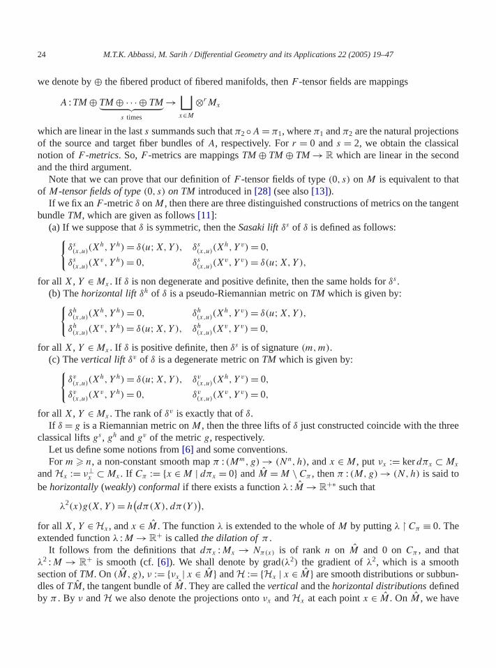
we denote by⊕ the fibered product of fibered manifolds, thenF -tensor fields are mappings

A : TM ⊕ TM ⊕ · · · ⊕ TM︸︷︷︸s times

→⊔x∈M

⊗rMx

which are linear in the lasts summands such thatπ2◦A = π1, whereπ1 andπ2 are the natural projectionof the source and target fiber bundles ofA, respectively. Forr = 0 ands = 2, we obtain the classicanotion ofF -metrics. So,F -metrics are mappingsTM ⊕ TM ⊕ TM → R which are linear in the seconand the third argument.

Note that we can prove that our definition ofF -tensor fields of type(0, s) on M is equivalent to thaof M-tensor fields of type(0, s) on TM introduced in[28] (see also[13]).

If we fix anF -metricδ onM , then there are three distinguished constructions of metrics on the tabundleTM, which are given as follows[11]:

(a) If we suppose thatδ is symmetric, then theSasaki liftδs of δ is defined as follows:{δs(x,u)(X

h,Y h) = δ(u;X,Y ), δs(x,u)(X

h,Y v) = 0,

δs(x,u)(X

v, Y h) = 0, δs(x,u)(X

v, Y v) = δ(u;X,Y ),

for all X, Y ∈ Mx . If δ is non degenerate and positive definite, then the same holds forδs .(b) Thehorizontal lift δh of δ is a pseudo-Riemannian metric onTM which is given by:{

δh(x,u)(X

h,Y h) = 0, δh(x,u)(X

h,Y v) = δ(u;X,Y ),

δh(x,u)(X

v, Y h) = δ(u;X,Y ), δh(x,u)(X

v, Y v) = 0,

for all X, Y ∈ Mx . If δ is positive definite, thenδs is of signature(m,m).(c) Thevertical lift δv of δ is a degenerate metric onTM which is given by:{

δv(x,u)(X

h,Y h) = δ(u;X,Y ), δv(x,u)(X

h,Y v) = 0,

δv(x,u)(X

v, Y h) = 0, δv(x,u)(X

v, Y v) = 0,

for all X, Y ∈ Mx . The rank ofδv is exactly that ofδ.If δ = g is a Riemannian metric onM , then the three lifts ofδ just constructed coincide with the thre

classical liftsgs , gh andgv of the metricg, respectively.Let us define some notions from[6] and some conventions.For m � n, a non-constant smooth mapπ : (Mm,g) → (Nn,h), andx ∈ M , put νx := kerdπx ⊂ Mx

andHx := ν⊥x ⊂ Mx . If Cπ := {x ∈ M | dπx = 0} andM = M \ Cπ , thenπ : (M,g) → (N,h) is said to

behorizontally(weakly) conformalif there exists a functionλ : M → R+∗ such that

λ2(x)g(X,Y ) = h(dπ(X), dπ(Y )

),

for all X, Y ∈Hx , andx ∈ M . The functionλ is extended to the whole ofM by puttingλ � Cπ ≡ 0. Theextended functionλ :M → R

+ is calledthe dilation ofπ .It follows from the definitions thatdπx :Mx → Nπ(x) is of rank n on M and 0 onCπ , and that

λ2 :M → R+ is smooth (cf.[6]). We shall denote by grad(λ2) the gradient ofλ2, which is a smooth

section ofTM. On(M, g), ν := {νx | x ∈ M} andH := {Hx | x ∈ M} are smooth distributions or subbudles ofTM, the tangent bundle ofM . They are called thevertical and thehorizontal distributionsdefinedby π . By ν andH we also denote the projections ontoνx andHx at each pointx ∈ M . On M , we have


y

al

nt dila-

n

e

l

s

thing

the unique orthogonal decomposition of the gradient ofλ2 into its vertical and horizontal parts given b

grad(λ2) = gradν(λ2) + gradH(λ2).

A non-constant smooth mapπ : (M,g) → (N,h) is said to behorizontally homotheticif it is horizon-tally conformal and gradH(λ2) ≡ 0 onM .

Note that in this caseπ is necessarily a Riemannian submersion up to a fixed homothety, i.e.M = M

(cf. [5]).The horizontal homothety is therefore equivalent toλ2 :M → R

+ being constant along horizontcurves in(M,g).

If furthermore gradν(λ2) ≡ 0 onM , then we say thatπ is strongly horizontally homothetic, or thatg

is strongly horizontally homothetic toh. In this caseλ2 is constant onM .Riemannian submersions are examples of strongly horizontally homothetic maps (with consta

tion λ2 ≡ 1). Another example is the following:Let (M,g) be a Riemannian manifold,TM its tangent bundle andG a Riemannian metric onTM.

If we take π as the canonical projectionpM : (TM,G) → (M,g), then it is easy to check thatG isstrongly horizontally homothetic tog if and only if there is a constantc � 0 such thatG(x,u)(X

h,Y h) =c.gx(X,Y ), for all vectorsX, Y ∈ Mx , x ∈ M , where the lifts are taken at a point(x, u) ∈ Mx . If c = 1,thenpM is a Riemannian submersion, and equivalently we shall say thatG is horizontally isometric tog.

1.2. g-natural metrics

Now, we shall describe all first order natural operatorsD :S2+T ∗ � (S2T ∗)T transforming Riemanniametrics on manifolds into metrics on their tangent bundles, whereS2+T ∗ andS2T ∗ denote the bundlefunctors of all Riemannian metrics and all symmetric two-forms overm-manifolds, respectively. For thconcept of naturality and related notions, see[9] for more details.

Let us call every sectionG : TM → (S2T ∗)TM a (possibly degenerate)metric. Then there is a bijectivecorrespondence between the triples of first order naturalF -metrics (ζ1, ζ2, ζ3) and first order natura(possibly degenerate) metricsG on the tangent bundles given by (cf.[11]):

G = ζ s1 + ζ h

2 + ζ v3 .

Therefore, to find all first order natural operatorsS2+T ∗ � (S2T ∗)T transforming Riemannian metricon manifolds into metrics on their tangent bundles, it suffices to describe all first order naturalF -metrics,i.e., first order natural operatorsS2+T ∗ � (T ,F ). In this sense, it is shown in[11] (see also[1,9]) that allfirst order naturalF -metricsζ in dimensionm > 1 form a family parametrized by two arbitrary smoofunctionsα0, β0 :R+ → R, whereR

+ denotes the set of all nonnegative real numbers, in the followway: For every Riemannian manifold(M,g) and tangent vectorsu, X, Y ∈ Mx

(1.12)ζ(M,g)(u)(X,Y ) = α0(g(u,u)

)g(X,Y ) + β0

(g(u,u)

)g(u,X)g(u,Y ).

If m = 1, then the same assertion holds, but we can always chooseβ0 = 0.In particular, all first order naturalF -metrics are symmetric.

Definition 1.1. Let (M,g) be a Riemannian manifold. We shall call a metricG onTM which comes fromg by a first order natural operatorS2+T ∗ � (S2T ∗)T ag-natural metric.


t

at

Thus, allg-natural metrics on the tangent bundle of a Riemannian manifold(M,g) are completelydetermined as follows:

Proposition 1.2 [3]. Let (M,g) be a Riemannian manifold andG be ag-natural metric on TM. Thenthere are functionsαi , βi :R+ → R, i = 1,2,3, such that for everyu, X, Y ∈ Mx , we have

(1.13)

G(x,u)(Xh,Y h) = (α1 + α3)(r

2)gx(X,Y ) + (β1 + β3)(r2)gx(X,u)gx(Y,u),

G(x,u)(Xh,Y v) = α2(r

2)gx(X,Y ) + β2(r2)gx(X,u)gx(Y,u),

G(x,u)(Xv, Y h) = α2(r


G(x,u)(Xv, Y v) = α1(r


wherer2 = gx(u,u).For m = 1, the same holds withβi = 0, i = 1,2,3.

Notations 1.3. In the sequel, we shall use the following notations:

• φi(t) = αi(t) + tβi(t),• α(t) = α1(t)(α1 + α3)(t) − α2

2(t),• φ(t) = φ1(t)(φ1 + φ3)(t) − φ22(t),

for all t ∈ R+.

Riemanniang-natural metrics are characterized as follows:

Proposition 1.4 [3]. The necessary and sufficient conditions for ag-natural metricG on the tangenbundle of a Riemannian manifold(M,g) to be Riemannian are that the functions ofProposition1.2,definingG, satisfy the inequalities

(1.14)

{α1(t) > 0, φ1(t) > 0,

α(t) > 0, φ(t) > 0,

for all t ∈ R+.

For m = 1 the system reduces toα1(t) > 0 andα(t) > 0, for all t ∈ R+.

Important Conventions.

(1) In the sequel, when we consider an arbitrary Riemanniang-natural metricG on TM, we implicitlysuppose that it is defined by the functionsαi , βi :R+ → R, i = 1,2,3, given inProposition 1.2andsatisfying(1.14).

(2) Unless otherwise stated, all real functionsαi , βi , φi , α andφ and their derivatives are evaluatedr2 := gx(u,u).

In [3], we have calculated the Levi-Civita connection∇ of an arbitraryg-natural metric onTM. Ourresult can be presented as follows:


Proposition 1.5. Let (M,g) be a Riemannian manifold,∇ its Levi-Civita connection andR its curvaturetensor. LetG be a Riemanniang-natural metric on TM. Then the Levi-Civita connection∇ of (TM,G)

is characterized by

(i) (∇XhY h)(x,u) = (∇XY )h(x,u) + h{A(u;Xx,Yx)} + v{B(u;Xx,Yx)},

(ii) (∇XhY v)(x,u) = (∇XY )v(x,u) + h{C(u;Xx,Yx)} + v{D(u;Xx,Yx)},

(iii) (∇XvY h)(x,u) = h{C(u;Yx,Xx)} + v{D(u;Yx,Xx)},(iv) (∇XvY v)(x,u) = h{E(u;Xx,Yx)} + v{F(u;Xx,Yx)},

for all vector fieldsX, Y on M and (x, u) ∈ TM, whereA, B, C, D, E andF are theF -tensor fields oftype(1,2) on M defined, for allu, X, Y ∈ Mx , x ∈ M , by:

A(u;X,Y ) = −α1α2

2α

[R(X,u)Y + R(Y,u)X

] + α2(β1 + β3)

2α

[gx(Y,u)X + gx(X,u)Y

]+ 1

αφ

{α2

[α1(φ1(β1 + β3) − φ2β2) + α2(β1α2

− β2α1)]gx(R(X,u)Y,u) + φ2α(α1 + α3)

′gx(X,Y )

+ [αφ2(β1 + β3)

′ + (β1 + β3)[α2(φ2β2 − φ1(β1 + β3))

+ (α1 + α3)(α1β2 − α2β1)]]

gx(X,u)gx(Y,u)}u,

B(u;X,Y ) = α22

αR(X,u)Y − α1(α1 + α3)

2αR(X,Y )u

− (α1 + α3)(β1 + β3)

2α

[gx(Y,u)X + gx(X,u)Y

]+ 1

αφ

{α2

[α2(φ2β2 − φ1(β1 + β3)) + (α1 + α3)(β2α1

− β1α2)]gx(R(X,u)Y,u) − α(φ1 + φ3)(α1 + α3)

′gx(X,Y )

+ [ − α(φ1 + φ3)(β1 + β3)′ + (β1 + β3)(α1 + α3)

[(φ1 + φ3)β1 − φ2β2

]+ α2

[α2(β1 + β3) − (α1 + α3)β2

]]gx(X,u)gx(Y,u)

}u,

C(u;X,Y ) = −α21

2αR(Y,u)X − α1(β1 + β3)

2αgx(X,u)Y

+ 1

α

[α1(α1 + α3)

′ − α2

(α′

2 − β2

2

)]gx(Y,u)X

+ 1

αφ

{α1

2

[α2(α2β1 − α1β2) + α1(φ1(β1 + β3)

− φ2β2)]gx(R(X,u)Y,u)+ α

[φ1

2(β1 + β3) + φ2

(α′

2 − β2

2

)]gx(X,Y )

+[αφ1(β1 + β3)

′ + [α2(α1β2 − α2β1)


+ α1(φ2β2 − (β1 + β3)φ1)][

(α1 + α3)′ + β1 + β3

2

]+ [

α2(β1(φ1 + φ3) − β2φ2) + α1(β2(α1 + α3))

− α2(β1 + β3)](

α′2 − β2

2

)]gx(X,u)gx(Y,u)

}u,

D(u;X,Y ) = 1

α

{α1α2

2R(Y,u)X − α2(β1 + β3)

2gx(X,u)Y

+[−α2(α1 + α3)

′ + (α1 + α3)

(α′

2 − β2

2

)]gx(Y,u)X

}

+ 1

αφ

{α1

2

[(α1 + α3)(α1β2 − α2β1) + α2(φ2β2 − φ1(β1 + β3))

]gx(R(X,u)Y,u)

− α

[φ2

2(β1 + β3) + (φ1 + φ3)

(α′

2 − β2

2

)]gx(X,Y )

+[αφ2(β1 + β3)

′ + [(α1 + α3)(α2β1 − α1β2)

+ α2(φ1(β1 + β3) − φ2β2)][

(α1 + α3)′ + β1 + β3

2

]+ [

(α1 + α3)(β2φ2 − β1(φ1 + φ3)) + α2(β2(α1 + α3))

− α2(β1 + β3)](

α′2 − β2

2

)]gx(X,u)gx(Y,u)

}u,

E(u;X,Y ) = 1

α

[α1

(α′

2 + β2

2

)− α2α

′1

][gx(Y,u)X + gx(X,u)Y

]+ 1

αφ

{α[φ1β2 − φ2(β1 − α′

1)]gx(X,Y )

+ [α(2φ1β

′2 − φ2β

′1) + 2α′

1

[α1(α2(β1 + β3)

− β2(α1 + α3)) + α2(β1(φ1 + φ3) − β2φ2)]

+ (2α′2 + β2)

[α1(φ2β2 − φ1(β1 + β3)) + α2(α1β2 − α2β1)

]]gx(X,u)gx(Y,u)

}u,

F (u;X,Y ) = 1

α

[−α2

(α′

2 + β2

2

)+ (α1 + α3)α

′1

][gx(Y,u)X + gx(X,u)Y

]+ 1

αφ

{α[(φ1 + φ3)(β1 − α′

1) − φ2β2]gx(X,Y )

+ [α((φ1 + φ3)β

′1 − 2φ2β

′2) + 2α′

1

[α2(β2(α1 + α3)

− α2(β1 + β3)) + (α1 + α3)(β2φ2 − β1(φ1 + φ3))]

+ (2α′2 + β2)

[α2(φ1(β1 + β3) − φ2β2)

+ (α1 + α3)(α2β1 − α1β2)]]

gx(X,u)gx(Y,u)}u.

For m = 1 the same holds withβi = 0, i = 1,2,3.


f

rite

2. Some notations and properties of F -tensor fields

Fix (x, u) ∈ TM and a system of normal coordinatesS := (U ;x1, . . . , xm) of (M,g) centered atx.Then we can define onU the vector field U:= ∑

i ui ∂

∂xi , where(u1, . . . , um) are the coordinates of(x, u)

with respect to the basis(( ∂

∂xi )x; i = 1, . . . ,m) of Mx .Let P be anF -tensor field of type(p, q) on M . Then, onU , we can define a(p, q)-tensor fieldP S

u

(or Pu if there is no risk of confusion), associated tou andS, by

(2.1)Pu(X1, . . . ,Xq) := P(Uz;X1, . . . ,Xq),

for all (X1, . . . ,Xq) ∈ Mz, z ∈ U .Informally, we can say that we have “tensorized” P atu with respect toS.On the other hand, if we fixx ∈ M andq vectorsX1, . . . ,Xq in Mx , then we can define aC∞-mapping

P(X1,...,Xq ) :Mx → ⊗pMx , associated to(X1, . . . ,Xq), by

(2.2)P(X1,...,Xq)(u) := P(u;X1, . . . ,Xq),

for all u ∈ Mx .Let s > t be two non-negative integers,T be a(1, s)-tensor field onM andP T be anF -tensor field,

of type(1, t), of the form

(2.3)P T (u;X1, . . . ,Xt) = T (X1, . . . , u, . . . , u, . . . ,Xt),

for all (u,X1, . . . ,Xt) ∈ TM⊕· · ·⊕ TM, i.e.,u appearss − t times at positionsi1, . . . , is−t in the expres-sion ofT . Then

– P Tu is a(1, t)-tensor field on a neighborhoodU of x in M , for all u ∈ Mx ;

– P T(X1,...,Xt )

is aC∞-mappingMx → Mx , for all X1, . . . ,Xt in Mx .

Furthermore, we have

Lemma 2.1. (1) The covariant derivative ofP Tu , with respect to the Levi-Civita connection of(M,g), is

given by:

(2.4)(∇XP T

u

)(X1, . . . ,Xt) = (∇XT )(X1, . . . , u, . . . , u, . . . ,Xt ),

for all vectorsX, X1, . . . ,Xt in Mx , whereu appears at positionsi1, . . . , is−t in the right-hand side othe preceding formula.

(2) The differential ofP T(X1,...,Xt )

, at u ∈ Mx , is given by:

(2.5)d(P T

(X1,...,Xt )

)u(X) = T (X1, . . . ,X, . . . , u, . . . ,Xt) + · · · + T (X1, . . . , u, . . . ,X, . . . ,Xt),

for all X ∈ Mx .

Proof. (1) If we extendX1, . . . ,Xt to vector fields onU denoted by the same letters, then we can w

(∇XP Tu )(X1, . . . ,Xt)

= ∇X

[P T

u (X1, . . . ,Xt )] − P T

u (∇XX1, . . . ,Xt) − · · · − P Tu (X1, . . . ,∇XXt)

= ∇X

[T (X1, . . . ,U, . . . ,U, . . . ,Xt)

] − T (∇XX1, . . . , u, . . . , u, . . . ,Xt)


led

−· · · − T (X1, . . . , u, . . . , u, . . . ,∇XXt)

= (∇XT )(X1, . . . , u, . . . , u, . . . ,Xt) + T (X1, . . . ,∇XU, . . . , u, . . . ,Xt)

+ · · · + T (X1, . . . , u, . . . ,∇XU, . . . ,Xt).

But ∇XU = ∑i u

i∇X∂

∂xi , sinceui is constant onU .On the other hand, the coordinate system(U ;x1, . . . , xm) is normal and hence

(2.6)Γ kij (x) = 0, i, j, k = 1, . . . ,m.

We deduce that∇X∂

∂xi = ∑i,j,k XjΓ k

ij (x) ∂

∂xk (x) = 0, where(Xi) are the components ofX with respectto the basis (( ∂

∂xi )x , i = 1, . . . ,m) of Mx . Hence

(2.7)∇XU = 0.

(2) P T(X1,...,Xt )

is the composite of an(s − t)-linear mappingMx × · · · × Mx → Mx and the diagonamappingMx → Mx × · · · × Mx , u → (u, . . . , u). A classical calculation gives obviously the requiridentity. �

We have also the following:

Lemma 2.2. LetT be a(1, s)-tensor field onM . Then

(1) ∇Xhh{T (X1, . . . , u, . . . , u, . . . ,Xt)

}= h

{(∇XP T

u )((X1)x, . . . , (Xt)x) + A(u;X,Tx(X1, . . . , u, . . . , u, . . . ,Xt))}

+ v{B(u;X,Tx(X1, . . . , u, . . . , u, . . . ,Xt))

},

(2) ∇Xvh{T (X1, . . . , u, . . . , u, . . . ,Xt)

}= h

{d(P T

((X1)x,...,(Xt )x))u(X) + C(u;Tx(X1, . . . , u, . . . , u, . . . ,Xt),X)}

+ v{D(u;Tx(X1, . . . , u, . . . , u, . . . ,Xt),X)

},

(3) ∇Xhv{T (X1, . . . , u, . . . , u, . . . ,Xt)

}= h

{C(u;X,Tx(X1, . . . , u, . . . , u, . . . ,Xt))

}+ v

{(∇XP T

u )((X1)x, . . . , (Xt)x) + D(u;X,Tx(X1, . . . , u, . . . , u, . . . ,Xt))},

(4) ∇Xvv{T (X1, . . . , u, . . . , u, . . . ,Xt)

}= h

{E(u;X,Tx(X1, . . . , u, . . . , u, . . . ,Xt))

}+ v

{d(P T

((X1)x ,...,(Xt )x))u(X)) + F(u;X,Tx(X1, . . . , u, . . . , u, . . . ,Xt ))},

for all vector fieldsX1, . . . ,Xt on M and X ∈ Mx , whereu appears at positionsi1, . . . , is−t in anyexpression ofT . Here,Xh andXv are taken at(x, u).

Proof. We shall prove only (1), the proof of the other identities being similar.


∇Xhh{T (X1, . . . , u, . . . , u, . . . ,Xt)

}=

∑λ1,...,λs−t

∇Xh

{uλ1 · · ·uλs−t

[T

(X1, . . . ,

∂

∂xλ1, . . . ,

∂

∂xλs−t, . . . ,Xt

)]h}

=∑

λ1,...,λs−t

{uλ1 · · ·uλs−t ∇Xh

[T

(X1, . . . ,

∂

∂xλ1, . . . ,

∂

∂xλs−t, . . . ,Xt

)]h

−∑

k

XjΓλk

jµkuλ1 · · ·uµk · · ·uλs−t

[T

(X1, . . . ,

∂

∂xλ1(x), . . . ,

∂

∂xλs−t(x), . . . ,Xt

)]h},

where we have used(1.10)in the second identity. But, by virtue of(2.6), we deduce

∇Xhh{T (X1, . . . , u, . . . , u, . . . ,Xt)

}=

∑λ1,...,λs−t

uλ1 · · ·uλs−t ∇Xh

[T

(X1, . . . ,

∂

∂xλ1, . . . ,

∂

∂xλs−t, . . . ,Xt

)]h

=∑

λ1,...,λs−t

uλ1 · · ·uλs−t

{[(∇XT )

(X1, . . . ,

∂

∂xλ1, . . . ,

∂

∂xλs−t, . . . ,Xt

)]h

+ h

{A

(u;X,Tx

(X1, . . . ,

∂

∂xλ1(x), . . . ,

∂

∂xλs−t(x), . . . ,Xt

))}

+ v

{B

(u;X,Tx

(X1, . . . ,

∂

∂xλ1(x), . . . ,

∂

∂xλs−t(x), . . . ,Xt

))}}

= [(∇XT )

(X1, . . . , u, . . . , u, . . . ,Xt

)]h + h{A

(u;X,Tx(X1, . . . , u, . . . , u, . . . ,Xt)

)}+ v

{B(u;X,Tx(X1, . . . , u, . . . , u, . . . ,Xt))

}= [

(∇XP Tu )(X1, . . . ,Xt)

]h + h{A(u;X,Tx(X1, . . . , u, . . . , u, . . . ,Xt ))

}+ v

{B(u;X,Tx(X1, . . . , u, . . . , u, . . . ,Xt))

},

where we have used in the last equality formula(2.4). �Now, letP be theF -tensor field of type(1, t) of the form

(2.8)P(u;X1, . . . ,Xt) =∑

i

f Pi (r2)Ti(X1, . . . , u, . . . , u, . . . ,Xt),

wherefi :R+ → R are real-valued functions onR+, and anyTi is a(1, si)-tensor field onM , si > t , withthesi ’s not necessarily equal. Then, we have

Lemma 2.3. LetP be anF -tensor field, of type(1, t), onM given by(2.8). Then

(1) (∇XPu)(X1, . . . ,Xt) =∑

f Pi (r2)(∇XTi)(X1, . . . , u, . . . , u, . . . ,Xt ),

i


(2) d(P(X1,...,Xt ))x(X) = 2∑

i

(f Pi )′(r2)g(X,u)Ti(X1, . . . , u, . . . , u, . . . ,Xt )

+∑

i

f Pi (r2)

{Ti(X1, . . . ,X, . . . , u, . . . ,Xt ) + · · ·

+ Ti(X1, . . . , u, . . . ,X, . . . ,Xt)},

for all u,X,X1, . . . ,Xt ∈ Mx .

Proof. (1) It is clearPu(X1, . . . ,Xt) = ∑i fi(r

2)P Tiu (X1, . . . ,Xt). We deduce that

(∇XPu)(X1, . . . ,Xt) = 2∑

i

(f Pi )′(r2)g(∇XU, u)P Ti

u (X1, . . . ,Xt )

+∑

i

f Pi (r2)(∇XP Ti

u )(X1, . . . ,Xt)

=∑

i

f Pi (r2)(∇XP Ti

u )(X1, . . . ,Xt ),

by virtue of(2.7). Using(2.4), we obtain the desired identity.(2) is obtained, in the same manner, using(2.5) instead of(2.4). �If we denote byh{P(u;X1, . . . ,Xt)} (respectivelyv{P(u;X1, . . . ,Xt )}) the quantity

(2.9)h{P(u;X1, . . . ,Xt)

} =∑

i

f Pi (r2)h

{Ti(X1, . . . , u, . . . , u, . . . ,Xt)

}(2.10)(respectivelyv

{P(u;X1, . . . ,Xt)

} =∑

i

f Pi (r2)v

{Ti(X1, . . . , u, . . . , u, . . . ,Xt )

}),

then we can assert

Lemma 2.4.

(1) ∇Xhh{P(u;X1, . . . ,Xt)

}= h

{(∇XPu)((X1)x, . . . , (Xt )x) + A(u;X,P (u; (X1)x, . . . , (Xt)x))

}+ v

{B(u;X,P (u; (X1)x, . . . , (Xt)x))

},

(2) ∇Xvh{P(u;X1, . . . ,Xt )

}= h

{d(P((X1)x,...,(Xt )x))u(X) + C(u;P(u; (X1)x, . . . , (Xt )x),X)

}+ v

{D(u;P(u; (X1)x, . . . , (Xt)x),X)

},

(3) ∇Xhv{P(u;X1, . . . ,Xt)

}= h

{C(u;X,P (u; (X1)x, . . . , (Xt)x))

}+ v

{(∇XPu)((X1)x, . . . , (Xt)x) + D(u;X,P (u; (X1)x, . . . , (Xt)x))

},

(4) ∇Xvv{P(u;X1, . . . ,Xt)

}= h

{E(u;X,P (u; (X1)x, . . . , (Xt )x))

}+ v

{d(P((X1)x ,...,(Xt )x))u(X)) + F(u;X,P (u; (X1)x, . . . , (Xt)x))

},

for all vector fieldsX1, . . . ,Xt on M andX ∈ Mx . HereXh andXv are taken at(x, u).


Proof. We shall give the proof of (1), the proof of the other identities being similar. We have by(2.9)

∇Xhh{P(u;X1, . . . ,Xt)

} =∑

i

Xh(fi(r

2))h{Ti((X1)x, . . . , u, . . . , u, . . . , (Xt )x)

}+

∑i

fi(r2)∇Xhh

{Ti(X1, . . . , u, . . .u, . . . ,Xt)

}=

∑i

fi(r2)∇Xhh

{Ti(X1, . . . , u, . . . u, . . . ,Xt)

},

by virtue of(1.4). Hence, due toLemma 2.2andProposition 1.5, we obtain

∇Xhh{P(u;X1, . . . ,Xt)

} =∑

i

fi(r2)

{h{(∇XP Ti

u )((X1)x, . . . , (Xt)x

)+ A

(u;X,Ti((X1)x, . . . , u, . . . , u, . . . , (Xt)x)

)}+ v

{B

(u;X,Ti((X1)x, . . . , u, . . . , u, . . . , (Xt)x)

)}}.

Using the linearity ofA andB and (1) ofLemma 2.3, we obtain the required formula.�Finally, the following lemma will be used in the proof ofTheorem 0.2:

Lemma 2.5. LetP be anF -tensor field, of type(1, t + s), of the form

(2.11)P(u;X1, . . . ,Xt+s) = T(u;X1, . . . ,Xt , S(u;Xt+1, . . . ,Xt+s)

),

whereT andS are F -tensor fields of types(1, t + 1) and(1, s), respectively. Then we have

(∇XPu)(X1, . . . ,Xt+s) = (∇XTu)(X1, . . . ,Xt, Su(Xt+1, . . . ,Xt+s)

)(2.12)+ Tu

(X1, . . . ,Xt, (∇XSu)(Xt+1, . . . ,Xt+s)

),

for all X1, . . . ,Xt+s ∈ Mx , x ∈ M .

Proof. Notice that, for eachu ∈ Mx , x ∈ M , the(1, t + s)-tensor fieldPu is a contraction of the(2, t +s + 1)-tensor fieldTu ⊗ Su, sayPu = C(Tu ⊗ Su). It follows that (cf.[8], I, p. 123)

∇XPu = ∇X

[C(Tu ⊗ Su)

] = C(∇XTu ⊗ Su) + C(Tu ⊗ ∇XSu),

which gives, clearly, the result.�

3. Riemannian curvatures of g-natural metrics

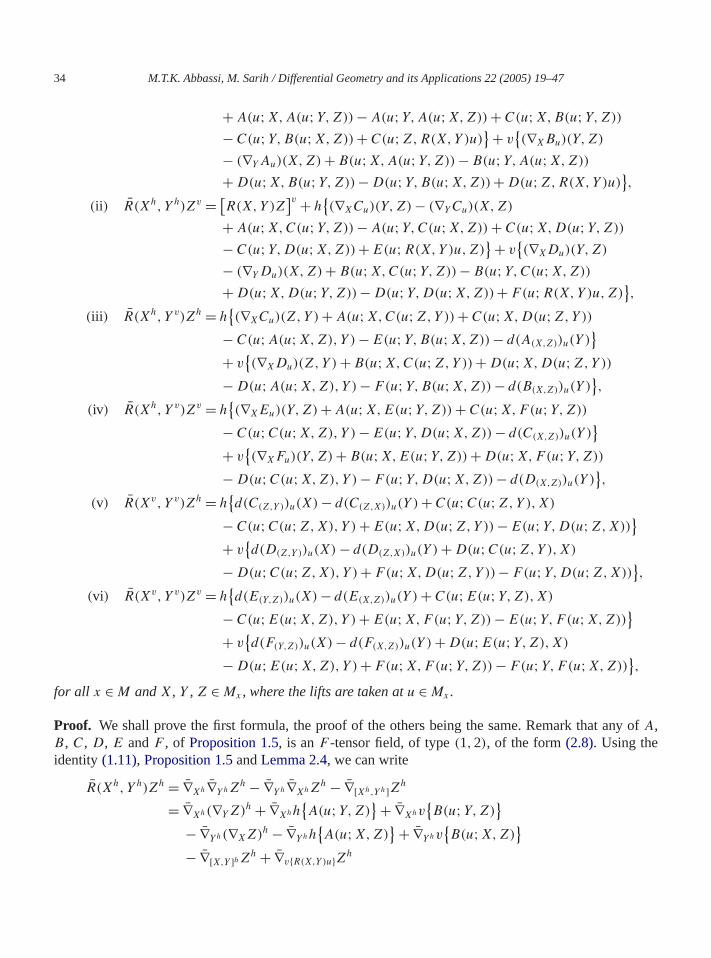
Proposition 3.1. Let (M,g) be a Riemannian manifold andG be a Riemanniang-natural metric onTM. Denote by∇ and R the Levi-Civita connection and the Riemannian curvature tensor of(M,g),respectively. Then, with the notations of Section2, the Riemannian curvature tensorR of (TM,G) iscompletely determined by

(i) R(Xh,Y h)Zh = [R(X,Y )Z

]h + h{(∇XAu)(Y,Z) − (∇Y Au)(X,Z)


of

+ A(u;X,A(u;Y,Z)) − A(u;Y,A(u;X,Z)) + C(u;X,B(u;Y,Z))

− C(u;Y,B(u;X,Z)) + C(u;Z,R(X,Y )u)}+ v

{(∇XBu)(Y,Z)

− (∇Y Au)(X,Z) + B(u;X,A(u;Y,Z)) − B(u;Y,A(u;X,Z))

+ D(u;X,B(u;Y,Z))− D(u;Y,B(u;X,Z))+ D(u;Z,R(X,Y )u)},

(ii) R(Xh,Y h)Zv = [R(X,Y )Z

]v + h{(∇XCu)(Y,Z) − (∇YCu)(X,Z)

+ A(u;X,C(u;Y,Z)) − A(u;Y,C(u;X,Z)) + C(u;X,D(u;Y,Z))

− C(u;Y,D(u;X,Z)) + E(u;R(X,Y )u,Z)} + v

{(∇XDu)(Y,Z)

− (∇Y Du)(X,Z) + B(u;X,C(u;Y,Z)) − B(u;Y,C(u;X,Z))

+ D(u;X,D(u;Y,Z))− D(u;Y,D(u;X,Z))+ F(u;R(X,Y )u,Z)},

(iii ) R(Xh,Y v)Zh = h{(∇XCu)(Z,Y ) + A(u;X,C(u;Z,Y )) + C(u;X,D(u;Z,Y ))

− C(u;A(u;X,Z),Y ) − E(u;Y,B(u;X,Z)) − d(A(X,Z))u(Y )}

+ v{(∇XDu)(Z,Y ) + B(u;X,C(u;Z,Y )) + D(u;X,D(u;Z,Y ))

− D(u;A(u;X,Z),Y ) − F(u;Y,B(u;X,Z)) − d(B(X,Z))u(Y )},

(iv) R(Xh,Y v)Zv = h{(∇XEu)(Y,Z) + A(u;X,E(u;Y,Z)) + C(u;X,F(u;Y,Z))

− C(u;C(u;X,Z),Y ) − E(u;Y,D(u;X,Z)) − d(C(X,Z))u(Y )}

+ v{(∇XFu)(Y,Z) + B(u;X,E(u;Y,Z)) + D(u;X,F(u;Y,Z))

− D(u;C(u;X,Z),Y ) − F(u;Y,D(u;X,Z)) − d(D(X,Z))u(Y )},

(v) R(Xv,Y v)Zh = h{d(C(Z,Y ))u(X) − d(C(Z,X))u(Y ) + C(u;C(u;Z,Y ),X)

− C(u;C(u;Z,X),Y ) + E(u;X,D(u;Z,Y )) − E(u;Y,D(u;Z,X))}

+ v{d(D(Z,Y ))u(X) − d(D(Z,X))u(Y ) + D(u;C(u;Z,Y ),X)

− D(u;C(u;Z,X),Y ) + F(u;X,D(u;Z,Y ))− F(u;Y,D(u;Z,X))},

(vi) R(Xv,Y v)Zv = h{d(E(Y,Z))u(X) − d(E(X,Z))u(Y ) + C(u;E(u;Y,Z),X)

− C(u;E(u;X,Z),Y ) + E(u;X,F(u;Y,Z)) − E(u;Y,F (u;X,Z))}

+ v{d(F(Y,Z))u(X) − d(F(X,Z))u(Y ) + D(u;E(u;Y,Z),X)

− D(u;E(u;X,Z),Y ) + F(u;X,F(u;Y,Z)) − F(u;Y,F (u;X,Z))},

for all x ∈ M andX, Y , Z ∈ Mx , where the lifts are taken atu ∈ Mx .

Proof. We shall prove the first formula, the proof of the others being the same. Remark that anyA,B, C, D, E andF , of Proposition 1.5, is anF -tensor field, of type(1,2), of the form(2.8). Using theidentity (1.11), Proposition 1.5andLemma 2.4, we can write

R(Xh,Y h)Zh = ∇Xh∇YhZh − ∇Yh∇XhZh − ∇[Xh,Yh]Zh

= ∇Xh(∇Y Z)h + ∇Xhh{A(u;Y,Z)

} + ∇Xhv{B(u;Y,Z)

}− ∇Yh(∇XZ)h − ∇Yhh

{A(u;X,Z)

} + ∇Yhv{B(u;X,Z)

}− ∇[X,Y ]hZh + ∇v{R(X,Y )u}Zh


,grk,

entities

f

= [R(X,Y )Z

]h + h{(∇XAu)(Y,Z) − (∇YAu)(X,Z)


− C(u;Y,B(u;X,Z)) + C(u;Z,R(X,Y )u)} + v

{(∇XBu)(Y,Z)


+ D(u;X,B(u;Y,Z)) − D(u;Y,B(u;X,Z))+ D(u;Z,R(X,Y )u)}. �

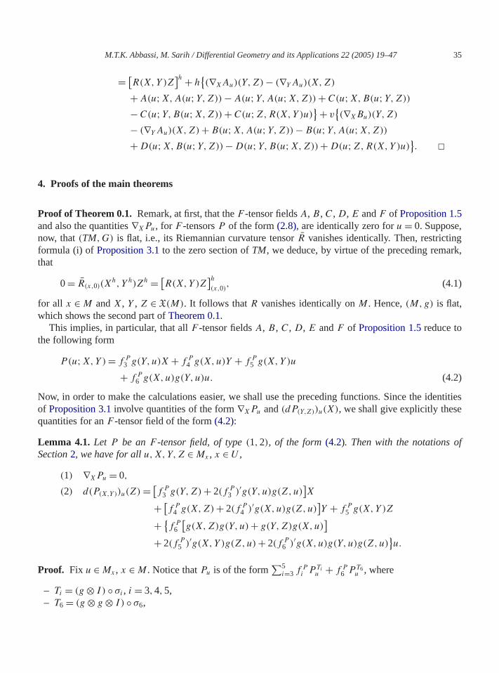
4. Proofs of the main theorems

Proof of Theorem 0.1. Remark, at first, that theF -tensor fieldsA, B, C, D, E andF of Proposition 1.5and also the quantities∇XPu, for F -tensorsP of the form(2.8), are identically zero foru = 0. Supposenow, that(TM,G) is flat, i.e., its Riemannian curvature tensorR vanishes identically. Then, restrictinformula (i) of Proposition 3.1to the zero section ofTM, we deduce, by virtue of the preceding remathat

(4.1)0= R(x,0)(Xh,Y h)Zh = [

R(X,Y )Z]h(x,0)

,

for all x ∈ M andX, Y , Z ∈ X(M). It follows thatR vanishes identically onM . Hence,(M,g) is flat,which shows the second part ofTheorem 0.1.

This implies, in particular, that allF -tensor fieldsA, B, C, D, E andF of Proposition 1.5reduce tothe following form

P(u;X,Y ) = f P3 g(Y,u)X + f P

4 g(X,u)Y + f P5 g(X,Y )u

(4.2)+ f P6 g(X,u)g(Y,u)u.

Now, in order to make the calculations easier, we shall use the preceding functions. Since the idof Proposition 3.1involve quantities of the form∇XPu and(dP(Y,Z))u(X), we shall give explicitly thesequantities for anF -tensor field of the form(4.2):

Lemma 4.1. Let P be anF -tensor field, of type(1,2), of the form(4.2). Then with the notations oSection2, we have for allu,X,Y,Z ∈ Mx , x ∈ U ,

(1) ∇XPu = 0,

(2) d(P(X,Y ))u(Z) = [f P

3 g(Y,Z) + 2(f P3 )′g(Y,u)g(Z,u)

]X

+ [f P

4 g(X,Z) + 2(f P4 )′g(X,u)g(Z,u)

]Y + f P

5 g(X,Y )Z

+ {f P

6

[g(X,Z)g(Y,u)+ g(Y,Z)g(X,u)

]+ 2(f P

5 )′g(X,Y )g(Z,u) + 2(f P6 )′g(X,u)g(Y,u)g(Z,u)

}u.

Proof. Fix u ∈ Mx , x ∈ M . Notice thatPu is of the form∑5

i=3 f Pi P Ti

u + f P6 P T6

u , where

– Ti = (g ⊗ I ) ◦ σi , i = 3,4,5,– T6 = (g ⊗ g ⊗ I ) ◦ σ6,


,

o

andσi are the mappings defined by

– σ3 :X1 ⊗ X2 ⊗ X3 → X1 ⊗ X3 ⊗ X2,– σ4 is the identity mapping,– σ5 :X1 ⊗ X2 ⊗ X3 → X2 ⊗ X3 ⊗ X1, and– σ6 :X1 ⊗ X2 ⊗ X3 → X1 ⊗ X2 ⊗ X1 ⊗ X3 ⊗ X1,

I being the identity(1,1)-tensor field onU . It follows that∇Ti = 0 onU , i = 3, . . . ,6, and consequentlyby virtue of (1) ofLemma 2.4, we obtain∇XP Ti

u = 0, for allX ∈ Mx . Using (1) ofLemma 2.3, we deducethat∇XPu = 0. The proof of the second property is similar, but usingLemmas 2.4 and 2.3. �

We shall now prove the first part ofTheorem 0.1, i.e., thatG is strongly horizontally homothetic tg. For this, it is sufficient to show, according to the first formula of(1.13), thatα1 + α3 is constant andβ1 + β3 vanishes identically onR+.

We shall start with the first property. In fact, if we putY = Z and we suppose that{u,X,Y } is anorthogonal system inMx , then for anyF -tensor fieldP of the form(4.2), we have:

P(u;X,Y ) = 0, P (u;X,u) = r2f P3 .X,

(4.3)P(u;u,X) = r2f P4 .X, P (u;X,X) = ‖X‖2f P

5 .u,

P (u;u,u) = r2[f P3 + f P

4 + f P5 + r2f P

6

]u.

Substituting from(4.3)and from the first identity ofLemma 4.1into (i) of Proposition 3.1, we obtain

R(x,u)(Xh,Y h)Y h = r2‖Y‖2[(f C

3 f B5 + f A

3 f A5

).Xh

u + (f B

3 f A5 + f D

3 f B5

).Xv

u

].

Consequently, we have onR+∗{f C

3 f B5 + f A

3 f A5 = 0,

f B3 f A

5 + f D3 f B

5 = 0.

Substituting fromProposition 1.5, we obtain onR+∗{α2Φ + α1Ψ = 0,

−(α1 + α3)Φ − α2Ψ = 0,

whereΦ = (α1 + α3)′[φ2

β1+β32 − (φ1 + φ3)(α

′2 − β2

2 )] andΨ = (φ1 + φ3)[(α1 + α3)′]2.

From the linear equations above we getΦ = Ψ = 0 (by virtue of α �= 0 everywhere). ButΨ = 0implies that(α1 + α3)

′ = 0 onR+∗, sinceφ1 + φ3 �= 0 everywhere. By continuity,(α1 + α3)

′ = 0 onR+.

We prove now thatβ1 +β3 vanishes identically onR+. In fact, if we putX = u andY = Z orthogonalto u, then substituting from analogous formulas of(4.3)and fromLemma 4.1into (i) of Proposition 3.1,we obtain

R(x,u)(uh, Y h)Y h = −r2‖Y‖2f B

4

[f E

5 .uh + f D5 .uh

].

Here, we have used the fact thatf A5 = f B

5 = 0 onR+, since(α1 +α3)

′ = 0 onR+. It follows that onR

+∗,we have{

f B4 f E

5 = 0,

f B4 f F

5 = 0.


Substituting fromProposition 1.5and using the facts thatα1 +α3 �= 0 andα �= 0 everywhere onR+∗, weobtain onR

+∗{(β1 + β3)[φ1

β1+β32 + φ2(α

′2 − β2

2 )] = 0,

(β1 + β3)[φ2β1+β3

2 + (φ1 + φ3)(α′2 − β2

2 )] = 0.

We claim thatβ1 + β3 = 0 everywhere onR+∗. Indeed, suppose that there is somet0 ∈ R+∗ such that

(β1 + β3)(t0) �= 0. Then the previous system reduces att0 to the system{φ1(t0)

β1+β32 (t0) + φ2(t0)(α

′2 − β2

2 )(t0) = 0,

φ2(t0)β1+β3

2 (t0) + (φ1 + φ3)(t0)(α′2 − β2

2 )(t0) = 0,

and hence, by virtue ofφ(t0) �= 0,

β1 + β3

2(t0) =

(α′

2 − β2

2

)(t0) = 0,

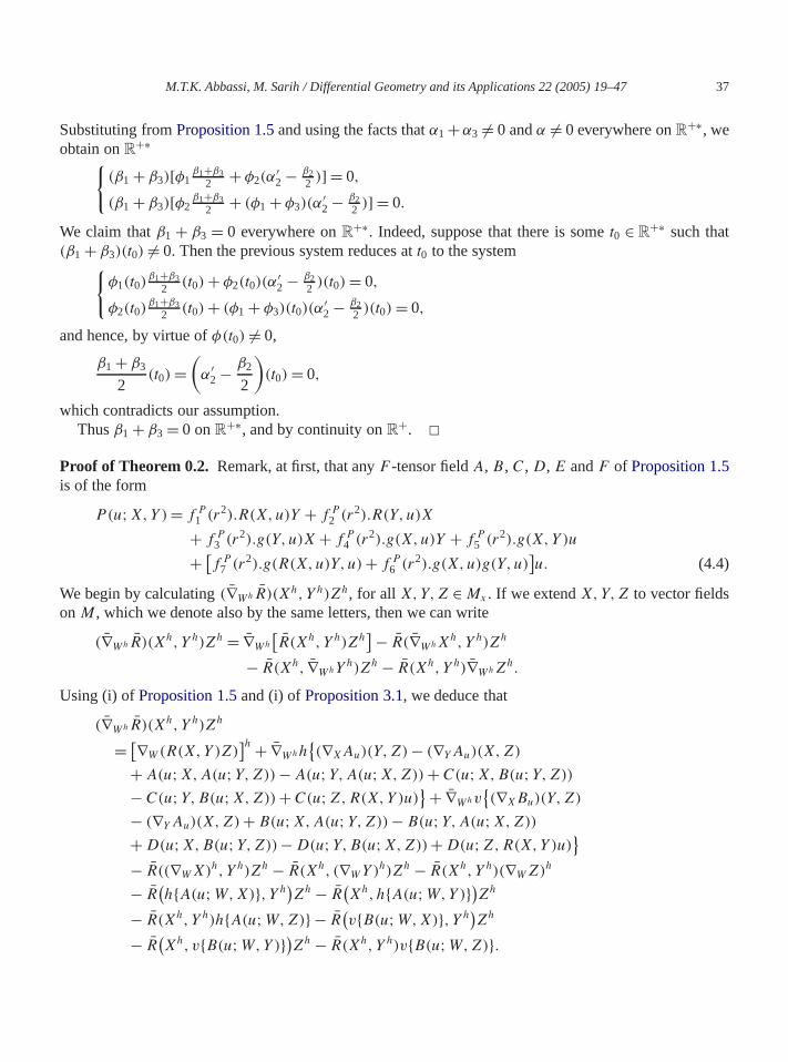
which contradicts our assumption.Thusβ1 + β3 = 0 onR

+∗, and by continuity onR+. �Proof of Theorem 0.2. Remark, at first, that anyF -tensor fieldA, B, C, D, E andF of Proposition 1.5is of the form

P(u;X,Y ) = f P1 (r2).R(X,u)Y + f P

2 (r2).R(Y,u)X

+ f P3 (r2).g(Y,u)X + f P

4 (r2).g(X,u)Y + f P5 (r2).g(X,Y )u

(4.4)+ [f P

7 (r2).g(R(X,u)Y,u) + f P6 (r2).g(X,u)g(Y,u)

]u.

We begin by calculating(∇WhR)(Xh,Y h)Zh, for all X,Y,Z ∈ Mx . If we extendX,Y,Z to vector fieldson M , which we denote also by the same letters, then we can write

(∇WhR)(Xh,Y h)Zh = ∇Wh

[R(Xh,Y h)Zh

] − R(∇WhXh,Y h)Zh

− R(Xh, ∇WhY h)Zh − R(Xh,Y h)∇WhZh.

Using (i) ofProposition 1.5and (i) ofProposition 3.1, we deduce that

(∇WhR)(Xh,Y h)Zh

= [∇W(R(X,Y )Z)]h + ∇Whh

{(∇XAu)(Y,Z) − (∇YAu)(X,Z)


− C(u;Y,B(u;X,Z)) + C(u;Z,R(X,Y )u)} + ∇Whv

{(∇XBu)(Y,Z)


+ D(u;X,B(u;Y,Z))− D(u;Y,B(u;X,Z))+ D(u;Z,R(X,Y )u)}

− R((∇WX)h,Y h)Zh − R(Xh, (∇WY )h)Zh − R(Xh,Y h)(∇WZ)h

− R(h{A(u;W,X)}, Y h

)Zh − R

(Xh,h{A(u;W,Y )})Zh

− R(Xh,Y h)h{A(u;W,Z)} − R(v{B(u;W,X)}, Y h

)Zh

− R(Xh, v{B(u;W,Y )})Zh − R(Xh,Y h)v{B(u;W,Z)}.


e

If we restrict ourselves to the zero section ofTM, then we can write, for eachF -tensor fieldP , of theform (4.4)

(4.5)P0 = 0.

We have, also, by (1) ofLemma 2.4and(4.5),[∇Whh{(∇XPu)(Y,Z)

}](x,0)

= [(∇W∇XP0)(Y,Z)

]h

(x,0)+ h

{A(0;W,(∇XP0)(Y,Z))

}+ v

{B(0;W,(∇XP0)(Y,Z))

}(4.6)= 0.

If P ′ is anotherF -tensor field of the form(4.4), then we obtain, using (1) ofLemma 2.4, (2.12)and(4.5)[∇Whh{P(u;X,P ′(u;Y,Z))

}](x,0)

= h{(∇WP0)(X,P ′

0(Y,Z)) + P0(X, (∇WP ′0)(Y,Z))

+ A(0;W,P (0;X,P ′(0;Y,Z))} + v

{B(0;W,P (0;X,P ′(0;Y,Z))

}(4.7)= 0.

Similarly, we have

(4.8)[∇Whv

{(∇XPu)(Y,Z)

}](x,0)

= 0 and

(4.9)[∇Whv

{P(u;X,P ′(u;Y,Z))

}](x,0)

= 0.

By virtue of (i) of Proposition 3.1and(4.5), we have

(4.10)R(x,0)

((∇WX)h,Y h

)Zh = [

R(∇WX,Y )Z]h

(x,0),

(4.11)R(x,0)

(Xh, (∇WY )h

)Zh = [

R(X,∇WY )Z]h

(x,0),

(4.12)R(x,0)(Xh,Y h)(∇WZ)h = [

R(X,Y )∇WZ]h

(x,0).

By a substitution from(4.5)–(4.12), we conclude that[(∇WhR)(Xh,Y h)Zh

](x,0)

= [∇W(R(X,Y )Z)]h

(x,0)− [

R(∇WX,Y )Z]h

(x,0)

− [R(X,∇WY )Z

]h

(x,0)− [

R(X,Y )∇WZ]h

(x,0).

It follows that

(4.13)[(∇WhR)(Xh,Y h)Zh

](x,0)

= [(∇WR)(X,Y )Z

]h

(x,0),

for all X,Y,Z,W ∈ Mx , x ∈ M . Hence, if we suppose that(TM,G) is locally symmetric, i.e.,∇R =0 identically, then we have, in particular, by virtue of(4.13), ∇R = 0 identically. This completes thproof. �Proof of Theorem 0.3. Let G be any Riemanniang-natural metric onTM.


ure

re.

We start by proving the heredity of the constant sectional curvature. Suppose that(TM,G) is a spaceof constant sectional curvatureK . Then we have, in particular,

(4.14)R(x,u)(Xh,Y h)Zh = K

(G(x,u)(Y

h,Zh)Xh − G(x,u)(Xh,Zh)Y h

),

for all X, Y , Z ∈ X(M) and(x, u) ∈ TM. If we takeu = 0 in (4.14)and we use the first identity of(1.13),then we get

(4.15)R(x,0)(Xh,Y h)Zh = K(α1 + α3)(0)

(gx(Y,Z)Xh

(x,0) − gx(X,Z)Y h(x,0)

).

Substituting from(4.1) into (4.15), we deduce that

(4.16)[R(X,Y )Z

]h

(x,0)= [

K(α1 + α3)(0)(gx(Y,Z)X − gx(X,Z)Y )]h

(x,0).

Since the mapX → Xh is an isomorphism between the vector spacesMx andH(x,0), formula (4.16)implies that

(4.17)Rx(X,Y )Z = K(α1 + α3)(0)(gx(Y,Z)X − gx(X,Z)Y

),

for all X, Y , Z ∈ X(M) andx ∈ M , which shows that(M,g) is a space of constant sectional curvatK(α1 + α3)(0).

We shall now prove the second part ofTheorem 0.3, i.e., the heredity of the constant scalar curvatuLet us evaluate the scalar curvatureS of (TM,G) at an arbitrary point(x,0) in the zero section ofTM,x ∈ M .

Notice that theF -tensor fieldsA, B, C, D, E andF , of Proposition 1.5, are of the form(4.4). For anarbitraryF -tensor field of the form(4.4), we have by virtue of (1) ofLemma 2.3and (1) ofLemma 4.1

(∇XPu)(Y,Z) = f P1 (∇XR)(Y,u)Z + f P

2 (∇XR)(Z,u)Y + f P7 g

((∇XR)(Y,u)Z,u

),

for all X,Y,Z andu ∈ Mx . It follows that

(4.18)∇XP0 = 0.

Also, we have, by virtue of (2) ofLemma 2.3and (2) ofLemma 4.1

d(P(X,Y ))u(Z) = 2g(Z,u){(f P

1 )′R(X,u)Y + (f P2 )′R(Y,u)X + (f P

3 )′g(Y,u)X

+ (f P4 )′g(X,u)Y + [

(f P5 )′g(X,Y ) + (f P

6 )′.g(X,u)g(Y,u)

+ (f P7 )′g(R(X,u)Y,u)

]u} + f P

1 R(X,Z)Y + f P2 R(Y,Z)X

+ f P3 g(Y,Z)X + f P

4 g(X,Z)Y + [f P

5 g(X,Y )

+ f P6 g(X,u)g(Y,u) + f P

7 g(R(X,u)Y,u)]X{

f P6

[g(X,Z)g(Y,u)+ g(Y,Z)g(X,u)

]+ f P

7

[g(R(X,Z)Y,u)+ g(R(X,u)Y,Z)

]}u,

for all X,Y,Z andu ∈ Mx . It follows that

d(P(Y,Z))0(X) = f P1 (0)R(Y,X)Z + f P

2 (0)R(Z,X)Y

(4.19)+ f P3 (0)g(X,Z)Y + f P

4 (0)g(X,Y )Z + f P5 (0)g(Y,Z)X.


n

Using(4.5), (4.18)and(4.19), we deduce fromPropositions 1.5 and 3.1that

(4.20)R(x,0)(Xh,Y h)Zh = [

R(X,Y )Z]h

,

R(x,0)(Xh,Y v)Zh = α2(0)

2α(0)h{α1(0)

[R(X,Y )Z + R(Z,Y )X)

]− (β1 + β3)(0)

[g(Y,Z)X + g(X,Y )Z

] − 2(α1 + α3)′(0)g(X,Z)Y

}+ 1

2α(0)v{−2(α2(0))2R(X,Y )Z + α1(0)(α1 + α3)(0)R(X,Z)Y

+ (α1 + α3)(0)(β1 + β3)(0)[g(Y,Z)X + g(X,Y )Z

](4.21)+ 2(α1 + α3)(0)(α1 + α3)

′(0)g(X,Z)Y},

R(x,0)(Xv, Y v)Zv = 1

α(0)

{h

{[−α1

(α′

2 − β2

2

)+ α2(2α′

1 − β1)

](0)

[g(Y,Z)X − g(X,Z)Y

]}

(4.22)

+ v

{[α2

(α′

2 − β2

2

)− (α1 + α3)(2α′

1 − β1)

](0)

[g(Y,Z)X − g(X,Z)Y

]}}.

Here, the lifts are taken at(x,0).Let {E1, . . . ,Em} be an orthonormal basis forMx . Then putting

Fi = 1√(α1 + α3)(0)

.Ehi and

(4.23)Fm+i = α2(0)√α(0)(α1 + α3)(0)

.Ehi −

√(α1 + α3)(0)√

α(0).Ev

i ; i = 1, . . . ,m,

we get an orthonormal basis{F1, . . . ,E2m} for the tangent space(TM)(x,0). Here, the lifts are also takeat (x,0). Note that eachFA, A = 1, . . . ,2m, is well-defined due to formulas(1.14).

The scalar curvatureS is, by definition, given by

S(x,0) =∑A,BA�=B

G(R(FA,FB)FB,FA

)

=∑i �=j

G(R(Fi,Fj )Fj ,Fi

) +∑i �=j

G(R(Fm+i , Fm+j )Fm+j ,Fm+i

)+ 2

∑i,j

G(R(Fi,Fm+j )Fm+j ,Fi

)

=∑i �=j

{1

((α1 + α3)(0))2

(1+ (α2(0))2

α(0)

)2

G(R(Eh

i ,Ehj )Eh

j ,Ehi

)

+ 2

α(0)

(1+ (α2(0))2

α(0)

)[ −2α2(0)

(α1 + α3)(0)G

(R(Eh

i ,Evj )E

hj ,Eh

i

)+ G

(R(Eh

i ,Evj )E

vj ,E

hi

)] + 2(α2(0))2

(α(0))2

[G

(R(Eh

i ,Ehj )Ev

j ,Evi

)


f

+ G(R(Eh

i ,Evj )E

hj ,Ev

i

)] − 2(α1 + α3)(0)

(α(0))2

[G

(R(Ev

i ,Evj )E

vj ,E

hi

)+ G

(R(Ev

i ,Evj )E

hj ,Ev

i

)] + ((α1 + α3)(0))2

(α(0))2G

(R(Ev

i ,Evj )E

vj ,E

vi

)}

+ 2

α(0)

∑i

G(R(Eh

i ,Evi )E

vi ,E

hi

).

Using the three formulas(4.20)–(4.22)of the Riemannian curvature tensorR(x,0) and the identities o(1.13), we find

G(x,0)

(R(Eh

i ,Ehj )Eh

j ,Ehi

) = (α1 + α3)(0)g(R(Ei,Ej )Ej ,Ei

),

G(x,0)

(R(Eh

i ,Evj )E

hj ,Eh

i

) = α2(0)g(R(Ei,Ej )Ej ,Ei

),

G(x,0)

(R(Eh

i ,Evj )E

vj ,E

hi

) = −(α1 + α3)′(0) − (β1 + β3)(0)(δij )

2,

G(x,0)

(R(Eh

i ,Ehj )Ev

j ,Evi

) = G(R(Eh

i ,Evj )E

hj ,Ev

i

) − G(R(Eh

j ,Evj )E

hi ,Ev

i

)= α1(0)g

(R(Ei,Ej )Ej ,Ei

),

G(x,0)

(R(Eh

i ,Evj )E

hj ,Ev

i

) = α1(0)

2g(R(Ei,Ej )Ej ,Ei

) + (β1 + β3)(0)

2

+[(β1 + β3)(0)

2+ (α1 + α3)

′(0)

](δij )

2,

G(x,0)

(R(Ev

i ,Evj )E

vj ,E

hi

) =[β2(0)

2− α′

2(0)

][1− (δij )

2],G(x,0)

(R(Ev

i ,Evj )E

hi ,Ev

j

) =[β2(0)

2− α′

2(0)

][1− (δij )

2],G(x,0)

(R(Ev

i ,Evj )E

vi ,E

vj

) = [β1(0) − 2α′

1(0)][

1− (δij )2].

Hence, by virtue of

1+ (α2(0))2

α(0)= α1(0)(α1 + α3)(0)

α(0)and S =

∑i �=j

g(R(Ei,Ej )Ej ,Ei

),

we deduce by simple calculation that

S(x,0) = α1(0)

α(0).Sx + m

(α(0))2

{−2[(m − 1)α1(0)(α1 + α3)(0)

+ α(0)](α1 + α3)

′(0) + [(m − 1)(α2(0))2 − 2α(0)

](β1 + β3)(0)

+ (m − 1)[((α1 + α3)(0))2(β1(0) − 2α′

1(0))

(4.24)− 2α2(0)(α1 + α3)(0)(β2(0) − 2α′2(0))

]},

whereS denotes the scalar curvature of(M,g).Now, if S is a constantS0 on TM, then in particular the functionx → S(x,0) is constant onM equal to

S0. It follows then from(4.24)thatS is constant. More precisely, we have

S = α(0)S0 − m {−2

[(m − 1)α1(0)(α1 + α3)(0) + α(0)

](α1 + α3)

′(0)
α1(0) α(0)α1(0)


is

+ [(m − 1)(α2(0))2 − 2α(0)

](β1 + β3)(0) + (m − 1)

[((α1 + α3)(0))2(β1(0)

− 2α′1(0)) − 2α2(0)(α1 + α3)(0)(β2(0) − 2α′

2(0))]}

. �Proof of Theorem 0.4. Fix x ∈ M . As in the proof ofTheorem 0.3, we consider the orthonormal bas{F1, . . . , F2m} of (TM)(x,0), given by(4.23), where{E1, . . . ,Em} is an orthonormal basis ofMx . Then theRicci tensor fieldRic of (TM,G) is, by definition, given by

(4.25)Ric(x,0)(V ,W) =m∑

i=1

[G(x,0)(R(V ,Fi)Fi,W) + G(x,0)(R(V ,Fm+i)Fm+i ,W)

],

for all V , W ∈ (TM)(x,0). If we putV = Xh andW = Y h, for X, Y ∈ Mx , then(4.25)becomes

Ric(x,0)(Xh,Y h) =

m∑i=1

{α1(0)

α(0)G(x,0)

(R(Xh,Eh

i )Ehi , Y h

)− α2(0)

α(0)

[G(x,0)(R(Xh,Eh

i )Evi , Y

h) + G(x,0)(R(Xh,Evi )E

hi , Y h)

](4.26)+ (α1 + α3)(0)

α(0)G(x,0)(R(Xh,Ev

i )Evi , Y

h)

}.

Using(4.20)and the first identity of(1.13), we obtain

(4.27)G(x,0)

(R(Xh,Eh

i )Ehi , Y h

) = (α1 + α3)(0)g(R(X,Ei)Ei, Y

).

Similarly, using(4.20)and the second identity of(1.13), we get

(4.28)G(x,0)

(R(Xh,Eh

i )Evi , Y

h) = α2(0)g

(R(X,Ei)Ei, Y

),

(4.29)G(x,0)

(R(Xh,Ev

i )Ehi , Y h

) = α2(0)g(R(X,Ei)Ei, Y

).

Finally, using(4.21)and the third identity of(1.13), we find

G(x,0)

(R(Xh,Ev

i )Evi , Y

h) = −G(x,0)

(R(Xh,Ev

i )Yh,Ev

i

)= −(α2(0))2

2α(0)

{2α1(0)g(R(X,Ei)Y,Ei) − 2(β1 + β3)(0)g(X,Ei)g(Y,Ei)

− 2(α1 + α3)′(0)g(X,Y )

} − α1(0)

2α(0)

{−2(α2(0))2g(R(X,Ei)Y,Ei)

+ 2(α1 + α3)(0)[(β1 + β3)(0)g(X,Ei)g(Y,Ei) + (α1 + α3)

′(0)g(X,Y )]}

.

It follows that

G(x,0)

(R(Xh,Ev

i )Evi , Y

h) = −(β1 + β3)(0)g(X,Ei)g(Y,Ei)

(4.30)− (α1 + α3)′(0)g(X,Y ).

Substituting from(4.27)–(4.30)into (4.26), we deduce that

Ric(x,0)(Xh,Y h) =

m∑{(α1(α1 + α3) − 2α2

2)(0)

α(0)g(R(X,Ei)Ei, Y

)
i=1


r

− (α1 + α3)(0)

α(0)

[(β1 + β3)(0)g(X,Ei)g(Y,Ei)

(4.31)+ (α1 + α3)′(0)g(X,Y )

]}.

But since{E1, . . . ,Em} is an orthonormal basis ofMx , then we havem∑

i=1

g(X,Ei)g(Y,Ei) = g(X,Y ).

It follows that

Ric(x,0)(Xh,Y h) = 1

α(0)

{(α1(α1 + α3) − 2α2

2)(0)

m∑i=1

g(R(X,Ei)Ei, Y )

(4.32)− (α1 + α3)(0)[(β1 + β3) + m(α1 + α3)

′](0)g(X,Y )

}.

If Ric denotes the Ricci tensor field of(M,g), then(4.32)transforms to

(4.33)

Ric(x,0)(Xh,Y h) = 1

α(0)

{(α1(α1 + α3) − 2α2

2)(0)Ricx(X,Y )

− (α1 + α3)(0)[(β1 + β3) + m(α1 + α3)

′](0)g(X,Y )}.

Now, if (TM,G) is an Einstein manifold, i.e.,Ric= λG, for a constantλ ∈ R, then we have in particula

(4.34)Ric(x,0)(Xh,Y h) = λG(x,0)(X

h,Y h) = λ(α1 + α3)(0)g(X,Y ),

for all x ∈ M andX, Y ∈ Mx .If we have(α1(α1 + α3) − 2α2

2)(0) �= 0, then substituting from(4.34)into (4.33), we deduce that

(4.35)Ricx(X,Y ) = (α1 + α3)[λα + (β1 + β3) + m(α1 + α3)′]

(α1(α1 + α3) − 2α22)

(0)gx(X,Y ),

for all x ∈ M andX, Y ∈ Mx . It follows that(M,g) is an Einstein manifold.If (α1(α1 + α3) − 2α2

2)(0) = 0, thenα(0) = (α2(0))2 and, in particular,α2(0) �= 0. By similar way asfor the computation ofRic(x,0)(X

h,Y h), we can calculateRic(x,0)(Xh,Y v) to find

(4.36)

Ric(x,0)(Xh,Y v) = 1

2α(0)

{−α1(0)α2(0)Ricx(X,Y )

+ [−α2(0)[(m + 1)(β1 + β3)(0) + 2(α1 + α3)

′(0)]

+ (m − 1)(α1 + α3)(0)(β2 − 2α′2)

]g(X,Y )

}.

Using the fact that(TM,G) is an Einstein manifold,(4.36)gives, by virtue ofα1(0) �= 0 andα2(0) �= 0,

Ricx(X,Y ) = 2

α1(0)α2(0)

{−λα(0)α2(0) + [−α2(0)[(m + 1)(β1 + β3)(0)

+ 2(α1 + α3)′(0)

] + (m − 1)(α1 + α3)(0)(β2 − 2α′2)

]}gx(X,Y ),

for all x ∈ M andX, Y ∈ Mx . It follows, also in this case, that(M,g) is an Einstein manifold. �
Proof of Theorem 0.5. It follows immediately fromTheorem A.2in Appendix Abelow. �


luable

s

Acknowledgements

The authors would like to thank Professor O. Kowalski and Professor L. Vanhecke for their vacomments and suggestions on this paper.

Appendix A

In [17], Oproiu defined a family of Riemannian metrics onTM, which depends on 2 arbitrary functionof one variable, in the following way:

For any two smooth functionsv,w :R+ → R, such thatv(t) > 0 andv(t)+2tw(t) > 0, for all t ∈ R+,

consider the metricGv,w on TM given locally by:

(A.1)Gv,w = ζ(u)ij dxi dxj + ξ(u)ij∇ui∇uj ,

where

(a) ζ (respectivelyξ ) is theF -metric onM defined by:

ζ(u;X,Y ) = v(τ)g(X,Y ) + w(τ)g(X,u)g(Y,u)

(respectivelyξ(u;X,Y ) = 1

v(τ)g(X,Y ) − w(τ)

v(τ)(v(τ) + 2tw(τ))g(X,u)g(Y,u)),

τ being the energy density, i.e.τ = 12g(u,u).

(b) ∇ui = dui +Γ ijku

jdxk is the absolute differential ofui with respect to the Levi-Civita connection∇of g.

It is easy to check thatGv,w is a Riemanniang-natural metric, where the defining functionsαi , βi ,i = 1,2,3, satisfy the following equalities:

(A.2)

(α1 + α3)(t) = v(t/2), (β1 + β3)(t) = w(t/2),

α1(t) = 1v(t/2)

, β1(t) = − w(t/2)

v(t/2)(v(t/2)+tw(t/2)),

α2(t) = β2(t) = 0,

for all t ∈ R+. Now, the following result was proved in[17] (see also[18]):

Theorem A.1. Let (M,g) be a space of negative constant sectional curvatureK and letv,w :R+ → R

be the functions given by:

(A.3)v(t) = A +√

A2 − 2Kt and w(t) = −2K

A+ K

A + √A2 − 2Kt

with A > 0.

Then(TM,Gv,w) is a Kaehler Einstein manifold.

Note thatTM, endowed with anyGv,w of Theorem A.1, is a locally symmetric space (cf.[19]).In the following theorem, we shall show additional properties of the metricsGv,w:


alarr

urent

ily

t

d

Theorem A.2. Let (M,g) be anm-dimensional space of negative constant sectional curvatureK , wherem � 3. Then, for any functionsv, w given by(A.3), the Riemanniang-natural metricGv,w provides TMwith a structure of a space of positive constant scalar curvature.

Further, for every choice of the constantsK < 0 and S0 > 0, there existsA > 0 such that the positiveconstant scalar curvature of(TM,Gv,w) is exactlyS0 > 0.

Proof. Suppose that(M,g) is a space of constant scalar curvatureK < 0. By virtue ofTheorem A.1,(TM,Gv,w) is an Einstein manifold, for anyv, w given by(A.3), and hence a space of constant sccurvatureS0. We claim thatS0 > 0. In fact, sinceα2 = β2 = 0, α(0) = α1(0)(α1 + α3)(0) and the scalacurvature of(M,g) is equal toS = m(m − 1)K , (4.24)reduces to

S0 = m(m − 1)

(α1 + α3)(0)K + m

(α(0))2

{−2mα(0)(α1 + α3)′(0)

(A.4)+ (m − 1)((α1 + α3)(0))2(β1(0) − 2α′1(0))

}.

On the other hand, a simple calculation, using(A.2) and (A.3), yields

α1(0) = 1

2A, (α1 + α3)(0) = 2A, α(0) = 1,

(α1 + α3)′(0) = v′(0)

2= − K

2A, β1(0) = − 3K

8A3,

α′1(0) = − v′(0)

2(v(0))2= K

8A3.

Substituting into(A.4), we find that

S0 = −m(m − 2)K

A,

which is positive form � 3, sinceK < 0.For an arbitrary constantS0 > 0, if we consider(M,g) a space of arbitrary constant sectional curvat

K < 0 andv, w given by(A.3), with A = −m(m−2)K

S0, then(TM,Gv,w) is, clearly, a space of consta

scalar curvatureS0. �Remarks A.3. (1) The family of Riemannian metrics onTM considered by Oproiu is, exactly, the famof Riemanniang-natural metrics onTM characterized by:

– horizontal and vertical distributions are orthogonal,– α = φ = 1.

Indeed, from(A.2), we haveα = α1(α1 + α3) = 1 andφ = φ1(φ1 + φ3) = (α1 + tβ1)((α1 + α3) + t (β1 +β3)) = 1. Conversely, ifα2 = β2 = 0 andα1, α1 + α3, β1 and β1 + β3 are given in such a way thaα = φ = 1, i.e., α1 = 1

α1+α3and φ1 = 1

φ1+φ3, then we definev and w by: v(t) = (α1 + α3)(2t) and

w(t) = (β1 + β3)(2t). It is easy to see, by virtue of(A.2), thatGv,w is no other than the metric defineby the givenαi , βi , i = 1,2,3, viaProposition 1.2.


re

ifold

)

riented

England,

okyo J.

Angew.

dles—a

bra und

3–195.

d Appli-

e form,

ppl. 11

¸

66..

(2) Let (M,g) be a space of negative constant sectional curvatureK . Anotherg-natural metric onTM,apart the Sasaki metric, which has vanishing scalar curvature is given by (cf.(4.24)):

(A.5)α1 = α1 + α3 = 1, α2 = β2 = 0, β1 = −K

1− Kt, β1 + β3 = −K.

In this case,(TM,G) is locally symmetric (Theorem 8 of[18]).(3) If, in the conditions of the preceding remark, we chooseK > 0, then we have also a structu

of locally symmetric Riemannian manifold, but in the tube around the zero section inTM, defined by‖u‖2 < 1

2K—not on wholeTM—(Theorem 8 of[18]).

References

[1] K.M.T. Abbassi, Note on the classification theorems ofg-natural metrics on the tangent bundle of a Riemannian man(M,g), Comment. Math. Univ. Carolinae, submitted for publication.

[2] K.M.T. Abbassi, M. Sarih, Killing vectorfields on tangent bundles with Cheeger–Gromoll metric, Tsukuba J. Math. 27 (2(2003) 295–306.

[3] K.M.T. Abbassi, M. Sarih, On natural metrics on tangent bundles of Riemannian manifolds,Arch. Math. (Brno), submittedfor publication.

[4] K.M.T. Abbassi, M. Sarih, The Levi-Civita connection of Riemannian natural metrics on the tangent bundle of an oRiemannian manifold, preprint.

[5] B. Fuglede, A criterion of non-vanishing differential of a smooth map, Bull. London Math. Soc. 14 (1982) 98–102.[6] S. Gudmundsson, The geometry of harmonic morphisms, Ph.D. Thesis in Pure Mathematics, University of Leeds,

April 1992.[7] S. Gudmundsson, E. Kappos, On the geometry of the tangent bundle with the Cheeger–Gromoll metric, T

Math. 14 (2) (2002) 407–717.[8] S. Kobayashi, K. Nomizu, Foundations of Differential Geometry, Intersci. Pub. New York (I, 1963 and II, 1967).[9] I. Kolár, P.W. Michor, J. Slovák, Natural Operations in Differential Geometry, Springer-Verlag, Berlin, 1993.

[10] O. Kowalski, Curvature of the induced Riemannian metric of the tangent bundle of Riemannian manifold, J. ReineMath. 250 (1971) 124–129.

[11] O. Kowalski, M. Sekizawa, Natural transformations of Riemannian metrics on manifolds to metrics on tangent bunclassification, Bull. Tokyo Gakugei Univ. (4) 40 (1988) 1–29.

[12] D. Krupka, J. Janyška, Lectures on Differential Invariants, University J.E. Purkyne, Brno, 1990.[13] K.P. Mok, E.M. Patterson, Y.C. Wong, Structure of symmetric tensors of type(0,2) and tensors of type(1,1) on the

tangent bundle, Trans. Amer. Math. Soc. 234 (1977) 253–278.[14] E. Musso, F. Tricerri, Riemannian metrics on tangent bundles, Ann. Math. Pura Appl. (4) 150 (1988) 1–20.[15] V. Oproiu, Some new geometric structures on the tangent bundle, Publ. Math. Debrecen 55 (1999) 261–281.[16] V. Oproiu, A locally symmetric Kähler Einstein structure on the tangent bundle of a space form, Beiträge zur Alge

Geometrie/Contributions to Algebra and Geometry 40 (1999) 363–372.[17] V. Oproiu, A Kähler Einstein structure on the tangent bundle of a space form, Int. J. Math. Math. Sci. 25 (2001) 18[18] V. Oproiu, Some Kähler structures on the tangent bundle of a space form, preprint.[19] V. Oproiu, N. Papaghiuc, Locally symmetric space structures on the tangent bundle, in: Differential Geometry an

cations, Satellite Conf. of ICM in Berlin, Aug. 10–14, 1998, Brno, Masaryk Univ. in Brno, 1999, pp. 99–109.[20] V. Oproiu, N. Papaghiuc, A locally symmetric Kähler Einstein structure on a tube in the tangent bundle of a spac

Rev. Roum. Math. Pures Appl. 45 (2000) 863–871.[21] V. Oproiu, N. Papaghiuc, A Kähler structure on the nonzero tangent bundle of a space form, Differential Geom. A

(1999) 1–12.[22] V. Oproiu, D.D. Poro¸sniuc, A Kähler Einstein structure on the cotangent bundle of a Riemannian manifold, An.Stiint.

Univ. Al. I. Cuza, Iasi, submitted for publication.[23] N. Papaghiuc, Another Kähler structure on the tangent bundle of a space form, Demonstratio Math. 31 (1998) 855–8[24] M. Sekizawa, Curvatures of tangent bundles with Cheeger–Gromoll metric, Tokyo J. Math. 14 (2) (1991) 407–717


ce form,

131–141.ama

in

a

3–443.

236.8 (2000)

okyo,

th.

1999)

,

01)

–354;

pecial or-

18 (2–3)

[25] M. Tahara, S. Marchiafava, Y. Watanabe, Quaterrnion Kähler structures on the tangent bundle of a complex spaRend. Istit. Mat. Univ. Trieste (Suppl.) 30 (1999) 163–175.

[26] M. Tahara, L. Vanhecke, Y. Watanabe, New structures on tangent bundles, Note di Matematica (Lecce) 18 (1998)[27] M. Tahara, Y. Watanabe, Natural almost Hermitian, Hermitian and Kähler metrics on the tangent bundles, Math. J. Toy

Univ. 20 (1997) 149–160.[28] Y.C. Wong, K.P. Mok, Connections andM-tensors on the tangent bundleTM, in: H. Rund, W.F. Forbes (Eds.), Topics

Differential Geometry, Academic Press, New York, 1959, pp. 157–172.

Further reading

K.M.T. Abbassi, M. Sarih, On Riemanniang-natural metrics of the forma.gs + b.gh + c.gv on the tangent bundle ofRiemannian manifold(M,g), preprint.

A.A. Borisenko, A.L. Yampol’skii, Riemannian geometry of fiber bundles, Russian Math. Surv. 46 (6) (1991) 55–106.J. Cheeger, D. Gromoll, On the structure of complete manifolds of nonnegative curvature, Ann. of Math. 96 (1972) 41P. Dombrowski, On the geometry of the tangent bundle, J. Reine Angew. Math. 210 (1962) 73–82.D.B.A. Epstein, Natural tensors on Riemannian manifolds, J. Differential Geometry 10 (1975) 631–645.D.B.A. Epstein, W.P. Thurston, Transformation groups and natural bundles, Proc. London Math. Soc. 38 (1979) 219–O. Kowalski, M. Sekizawa, On tangent sphere bundles with small or large constant radius, Ann. Global Anal. Geom. 1

207–219.A. Nijenhuis, Natural bundles and their general properties, in: Differential Geometry in Honor of K. Yano, Kinokuniya, T

1972, pp. 317–334.V. Oproiu, General natural almost Hermitian and anti-Hermitian structures on the tangent bundle, Bull. Soc. Sci. Ma

Roum. 43 (91) (2000) 325–340.V. Oproiu, A generalization of naturalalmost Hermitian structures on the tangent bundles, Math. J. Toyama Univ. 22 (

1–14.V. Oproiu, N. Papaghiuc, A pseudo-Riemannian metric on the cotangent bundle, An. ¸Stiint. Univ. Al. I. Cuza, Iasi 36 (1990)

265–276.V. Oproiu, N. Papaghiuc, Another pseudo-Riemannian metric on the cotangent bundle, Bull. Inst. Polit., Ia¸si 27 (1991), fasc.1-4

sect.1.R.S. Palais, C.L. Terng, Natural bundles have finite order, Topology 16 (1977) 271–277.N. Papaghiuc, A Ricci-flat pseudo-Riemannian metric on the tangent bundle of a Riemannian manifold, Coll. Math. 87 (20

227–233.S. Sasaki, On the differential geometry of tangent bundles of Riemannian manifolds, Tohôku Math. J. I 10 (1958) 338

Tohôku Math. J. II 14 (1962) 146–155.J. Slovák, On natural connections on Riemannian manifolds, Comment. Math. Univ. Carolinae 30 (1989) 389–393.P. Stredder, Natural differential operators on Riemannian manifolds and representations of the orthogonal and the s

thogonal groups, J. Differential Geometry 10 (1975) 647–660.C.L. Terng, Natural vector bundles and natural differential operators, Amer. J. Math. 100 (1978) 775–828.T.J. Willmore, An Introduction to Differential Geometry, Oxford Univ. Press, 1959.K. Yano, S. Ishihara, Tangent and cotangent bundles, Differential Geometry, Marcel Dekker Inc., New York, 1973.K. Yano, S. Kobayashi, Prolongations of tensor fields and connections to tangent bundles, J. Math. Soc. Japan (I, II)

(1966); J. Math. Soc. Japan (III) 19 (1967).

on some hereditary properties of riemannian -natural ...nice examples and counterexamples of several...

Documents