on the computational complexity of mathematical functions -...
TRANSCRIPT

On the computational complexity
of mathematical functions
Jean-Pierre Demailly
Institut Fourier, Universite de Grenoble I& Academie des Sciences, Paris (France)
November 26, 2011KVPY conference at Vijyoshi Camp
Jean-Pierre Demailly (Grenoble I), November 26, 2011 On the computational complexity of mathematical functions

Computing, a very old concern
Babylonian mathematical tabletallowing the computation of
√2
(1800 – 1600 BC)
Decimal numeral systeminvented in India (∼ 500BC ?) :
Jean-Pierre Demailly (Grenoble I), November 26, 2011 On the computational complexity of mathematical functions

Madhava’s formula for π
Early calculations of π were done by Greek and Indianmathematicians several centuries BC.
Jean-Pierre Demailly (Grenoble I), November 26, 2011 On the computational complexity of mathematical functions

Madhava’s formula for π
Early calculations of π were done by Greek and Indianmathematicians several centuries BC.These early evaluations used polygon approximations andPythagoras theorem. In this way, using 96 sides, Archimedesgot 3 + 10
71< π < 3 + 10
70whose average is 3.1418 (c. 230 BC).
Chinese mathematicians reached 7 decimal places in 480 AD.
The next progress was the discovery of the first infinite seriesformula by Madhava (circa 1350 – 1450), a prominentmathematician-astronomer from Kerala (formula rediscoveredin the XVIIe century by Leibniz and Gregory) :
π
4= 1− 1
3+
1
5− 1
7+
1
9− 1
11+ · · ·+ (−1)n
2n + 1+ · · ·
Convergence is unfortunately very slow, but Madhava was ableto improve convergence and reached in this way 11 decimal places.
Jean-Pierre Demailly (Grenoble I), November 26, 2011 On the computational complexity of mathematical functions

Ramanujan’s formula for π
Srinivasa Ramanujan (1887 – 1920),a self-taught mathematical prodigee.His work dealt mainly witharithmetics and function theory
1
π=
2√2
9801
+∞∑
n=0
(4n)!(1103 + 26390n)
(n!)43964n(1910).
Each term is approximately 108 times smaller than thepreceding one, so the convergence is very fast.
Jean-Pierre Demailly (Grenoble I), November 26, 2011 On the computational complexity of mathematical functions

Computational complexity theory
• Complexity theory is a branch of computer science andmathematics that :– tries to classify problems according to their difficulty– focuses on the number of steps (or time) needed to solve them.
• Let N = size of the data (e.g. for a decimal number, thenumber N of digits.)
A problem will be said to have polynomial complexity if itrequires less than C Nd steps (or units of time) to be solved,where C and d are constants (d is the degree).
• Especially, it is said to have– linear complexity when # steps ≤ C N
Jean-Pierre Demailly (Grenoble I), November 26, 2011 On the computational complexity of mathematical functions
Computational complexity theory
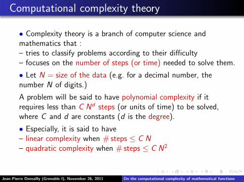
• Complexity theory is a branch of computer science andmathematics that :– tries to classify problems according to their difficulty– focuses on the number of steps (or time) needed to solve them.
• Let N = size of the data (e.g. for a decimal number, thenumber N of digits.)
A problem will be said to have polynomial complexity if itrequires less than C Nd steps (or units of time) to be solved,where C and d are constants (d is the degree).
• Especially, it is said to have– linear complexity when # steps ≤ C N
– quadratic complexity when # steps ≤ C N2
Jean-Pierre Demailly (Grenoble I), November 26, 2011 On the computational complexity of mathematical functions
Computational complexity theory
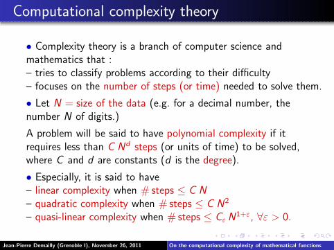
• Complexity theory is a branch of computer science andmathematics that :– tries to classify problems according to their difficulty– focuses on the number of steps (or time) needed to solve them.
• Let N = size of the data (e.g. for a decimal number, thenumber N of digits.)
A problem will be said to have polynomial complexity if itrequires less than C Nd steps (or units of time) to be solved,where C and d are constants (d is the degree).
• Especially, it is said to have– linear complexity when # steps ≤ C N
– quadratic complexity when # steps ≤ C N2
– quasi-linear complexity when # steps ≤ Cε N1+ε, ∀ε > 0.
Jean-Pierre Demailly (Grenoble I), November 26, 2011 On the computational complexity of mathematical functions

First observations about complexity
• Addition has linear complexity:consider decimal numbers of the form 0.a1a2a3 . . . aN ,0.b1b2b3 . . . bN , we have
∑
1≤n≤N
an10−n +
∑
1≤n≤N
bn10−n =
∑
1≤n≤N
(an + bn)10−n,
taking carries into account, this is done in N steps at most.
• What about multiplication ?
Jean-Pierre Demailly (Grenoble I), November 26, 2011 On the computational complexity of mathematical functions

First observations about complexity
• Addition has linear complexity:consider decimal numbers of the form 0.a1a2a3 . . . aN ,0.b1b2b3 . . . bN , we have
∑
1≤n≤N
an10−n +
∑
1≤n≤N
bn10−n =
∑
1≤n≤N
(an + bn)10−n,
taking carries into account, this is done in N steps at most.
• What about multiplication ?∑
1≤k≤N
ak10−k×
∑
1≤ℓ≤N
bℓ10−ℓ =
∑
1≤n≤N
cn10−n, cn =
∑
k+ℓ=n
akbℓ.
Calculation of each cn requires at most N elementarymultiplications and N − 1 additions and corresponding carries,thus the algorithm requires less than N × 3N steps.
Thus multiplication has at most quadratic complexity.Jean-Pierre Demailly (Grenoble I), November 26, 2011 On the computational complexity of mathematical functions

The Karatsuba algorithm
Can one do better than quadratic complexity for multiplication?
Jean-Pierre Demailly (Grenoble I), November 26, 2011 On the computational complexity of mathematical functions

The Karatsuba algorithm
Can one do better than quadratic complexity for multiplication?
Yes !! It was discovered by Karatsuba around 1960 thatmultiplication has complexity less than C N log2 3 ≃ C N1.585
Karatsuba’s idea: for N = 2q even, split x = 0.a1a2 . . . aN as
x = x ′ + 10−qx ′′, x ′ = 0.a1a2 . . . aq, x ′′ = 0.aq+1aq+2 . . . a2q
and similarly y = 0.b1b2 . . . bN = y ′ + 10−qy ′′. To calculatexy , one would normally need x ′y ′, x ′′y ′′ and x ′y ′′ + x ′′y ′ whichtake 4 multiplications and 1 addition of q-digit numbers.However, one can use only 3 multiplications by calculating
x ′y ′, x ′′y ′′, x ′y ′′ + x ′′y ′ = x ′y ′ + x ′′y ′′ − (x ′ − x ′′)(y ′ − y ′′)
(at the expense of 4 additions).
Jean-Pierre Demailly (Grenoble I), November 26, 2011 On the computational complexity of mathematical functions

The Karatsuba algorithm
Can one do better than quadratic complexity for multiplication?
Yes !! It was discovered by Karatsuba around 1960 thatmultiplication has complexity less than C N log2 3 ≃ C N1.585
Karatsuba’s idea: for N = 2q even, split x = 0.a1a2 . . . aN as
x = x ′ + 10−qx ′′, x ′ = 0.a1a2 . . . aq, x ′′ = 0.aq+1aq+2 . . . a2q
and similarly y = 0.b1b2 . . . bN = y ′ + 10−qy ′′. To calculatexy , one would normally need x ′y ′, x ′′y ′′ and x ′y ′′ + x ′′y ′ whichtake 4 multiplications and 1 addition of q-digit numbers.However, one can use only 3 multiplications by calculating
x ′y ′, x ′′y ′′, x ′y ′′ + x ′′y ′ = x ′y ′ + x ′′y ′′ − (x ′ − x ′′)(y ′ − y ′′)
(at the expense of 4 additions). One then proceeds inductivelyto conclude that the time T (N) needed for N = 2s satisfies
T (2s) ≤ 3T (2s−1) + 4 2s−1.
Jean-Pierre Demailly (Grenoble I), November 26, 2011 On the computational complexity of mathematical functions

Optimal complexity of multiplication
It is an easy exercise to conclude by induction thatT (2s) ≤ 6 3s − 4 2s if one assumes T (1) = 1, and so
T (2s) ≤ 6 3s ⇒ T (N) ≤ C N log2 3.
Jean-Pierre Demailly (Grenoble I), November 26, 2011 On the computational complexity of mathematical functions

Optimal complexity of multiplication
It is an easy exercise to conclude by induction thatT (2s) ≤ 6 3s − 4 2s if one assumes T (1) = 1, and so
T (2s) ≤ 6 3s ⇒ T (N) ≤ C N log2 3.
It was in fact shown in 1971 by Schonage and Strassen thatmultiplication has quasi-linear complexity, less than
C N logN log logN.
For this reason, the usual mathematical functions also havequasi-linear complexity at most !
The Schonage-Strassen algorithm is based on the use ofdiscrete Fourier transforms. The theory comes from JosephFourier, the founder of my university in 1810 ...
Jean-Pierre Demailly (Grenoble I), November 26, 2011 On the computational complexity of mathematical functions

Joseph Fourier
Joseph Fourier (1768 – 1830)in his suit of member ofAcademie des Sciences,of which he became“Secretaire Perpetuel”(Head) in 1822.
Jean-Pierre Demailly (Grenoble I), November 26, 2011 On the computational complexity of mathematical functions

Life of Joseph Fourier
Born in 1768 in a poor family, Joseph Fourier quickly revealshimself to be a scientific prodigee.
Jean-Pierre Demailly (Grenoble I), November 26, 2011 On the computational complexity of mathematical functions

Life of Joseph Fourier
Born in 1768 in a poor family, Joseph Fourier quickly revealshimself to be a scientific prodigee.
Orphan from mother at age 8 and from father at age 10, he issent to a religious military school in the city of Auxerre, wherehe has fortunately access to some important scientific books.
Jean-Pierre Demailly (Grenoble I), November 26, 2011 On the computational complexity of mathematical functions
Life of Joseph Fourier
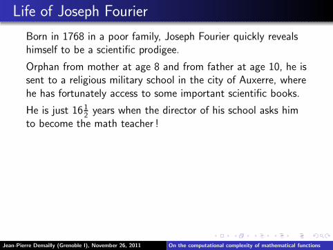
Born in 1768 in a poor family, Joseph Fourier quickly revealshimself to be a scientific prodigee.
Orphan from mother at age 8 and from father at age 10, he issent to a religious military school in the city of Auxerre, wherehe has fortunately access to some important scientific books.
He is just 1612years when the director of his school asks him
to become the math teacher !
Jean-Pierre Demailly (Grenoble I), November 26, 2011 On the computational complexity of mathematical functions

Life of Joseph Fourier
Born in 1768 in a poor family, Joseph Fourier quickly revealshimself to be a scientific prodigee.
Orphan from mother at age 8 and from father at age 10, he issent to a religious military school in the city of Auxerre, wherehe has fortunately access to some important scientific books.
He is just 1612years when the director of his school asks him
to become the math teacher !
At age 26, he becomes a Professor at Ecole Normale Superieureand Ecole Polytechnique. In 1798, he is chosen by Napoleonas his main scientific advisor during the campaign of Egypt.
Back in France in 1802, he becomes the Governor of theGrenoble area and founds the University. During this period,he discovers the heat equation and what is now called Fourieranalysis...
In 1824, he predicts the green house effect !Jean-Pierre Demailly (Grenoble I), November 26, 2011 On the computational complexity of mathematical functions

Heat equation and Fourier series
Let θ(x , y , z , t) be the the temperature of a physical materialat a point (x , y , z) and at time t.
Jean-Pierre Demailly (Grenoble I), November 26, 2011 On the computational complexity of mathematical functions

Heat equation and Fourier series
Let θ(x , y , z , t) be the the temperature of a physical materialat a point (x , y , z) and at time t.
Fourier shows theoretically and experimentally around 1807that θ(x , y , z , t) satisfies the propagation equation
θ′t = D(θ′′xx + θ′′yy + θ′′zz).
where D is a constant characterizing the material.
He then shows that in many cases the solutions can beexpressed in terms of trigonometric series
f (x) =+∞∑
n=0
an cos nωx + bn sin nωx =+∞∑
n=−∞
cneinωx
In fact all periodic phenomena can be described in this way.This is the basis of the modern theory of signal processing andelectromagnetism.
Jean-Pierre Demailly (Grenoble I), November 26, 2011 On the computational complexity of mathematical functions

Discrete Fourier transform
Let (an)0≤n<N be a finite sequence of numbers and let u be aprimitive N-th root of unity, i.e.
uN = 1 but un 6= 1 for 0 < n < N .
Jean-Pierre Demailly (Grenoble I), November 26, 2011 On the computational complexity of mathematical functions
Discrete Fourier transform
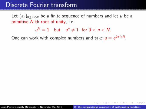
Let (an)0≤n<N be a finite sequence of numbers and let u be aprimitive N-th root of unity, i.e.
uN = 1 but un 6= 1 for 0 < n < N .
One can work with complex numbers and take u = e2πi/N .
Jean-Pierre Demailly (Grenoble I), November 26, 2011 On the computational complexity of mathematical functions

Discrete Fourier transform
Let (an)0≤n<N be a finite sequence of numbers and let u be aprimitive N-th root of unity, i.e.
uN = 1 but un 6= 1 for 0 < n < N .
One can work with complex numbers and take u = e2πi/N .
When working with integers, it is easier to work modulo alarge prime number, e.g. p = 65537 and takeN = p − 1 = 65536. Then u = 3 satisfies uN = 1 mod p andone can check that u = 3 is a primitive N-root of unity.
The discrete Fourier transform of (an) is the sequence
an =N−1∑
k=0
akukn.
It is convenient to consider that the index n is defined mod N
(e.g. a−n means aN−n for 0 < n < N).Jean-Pierre Demailly (Grenoble I), November 26, 2011 On the computational complexity of mathematical functions

Main formulas of Fourier theory
Fourier transform of a convolution:For a = (an) and b = (bn) define c = a ∗ b to be the sequence
cn =∑
p+q=n mod N
apbq “convolution of a and b.”
Then cn = anbn.
Jean-Pierre Demailly (Grenoble I), November 26, 2011 On the computational complexity of mathematical functions

Main formulas of Fourier theory
Fourier transform of a convolution:For a = (an) and b = (bn) define c = a ∗ b to be the sequence
cn =∑
p+q=n mod N
apbq “convolution of a and b.”
Then cn = anbn.
Proof.∑
s
csusn =
∑
s
( ∑
k+ℓ=s
akbℓ
)usn =
∑
k,ℓ
akuknbℓu
ℓn = anbn.
Fourier inversion formula: applying twice the Fouriertransform, one gets
an = N a−n = −a−n mod p (recall N = p − 1).
Proof. an =∑
k
(∑
ℓ
aℓukℓ)ukn =
∑
ℓ
aℓ
(∑
k
uk(n+ℓ))and
∑kuk(n+ℓ) = 0 if ℓ 6= −n and
∑kuk(n+ℓ) = N if ℓ = −n.
Jean-Pierre Demailly (Grenoble I), November 26, 2011 On the computational complexity of mathematical functions

Fast Fourier Transform (FFT)
Consequence: To calculate the convolution c = a ∗ b (which iswhat we need to calculate
∑ak10
−k∑
bℓ10−ℓ), one
calculates the Fourier transforms (an), (bn), then cn = anbn,which gives back (−c−n) and thus (cn) by Fourier inversion.
This looks complicated, but the Fourier transform can becomputed extremely fast !!
FFT algorithm: assume that N = 2s (in our exampleN = 65536 = 216) and define inductively αn,0 = an and
αn,k+1 = αn,k + αn+2ku2kn, 0 ≤ k < s.
By considering the binary decomposition n =∑
nk2k , 0 ≤ k < s,
of any integer n = 0...N − 1, one sees that αn,s = an. Thecalculation requires only s steps, each of which requires Nadditions and 2N mutiplications (using u2k+1n = (u2kn)2), so intotal we consume only 3sN = 3N log2 N operations !
Jean-Pierre Demailly (Grenoble I), November 26, 2011 On the computational complexity of mathematical functions

Other mathematical functions
OK about multiplication, but what for division ? square root ?
Jean-Pierre Demailly (Grenoble I), November 26, 2011 On the computational complexity of mathematical functions

Other mathematical functions
OK about multiplication, but what for division ? square root ?
Approximate division can be obtained solely from multiplication!If x0 is a rough approximation of 1/a, then the sequence
xn+1 = 2xn − ax2n
satisfies 1− axn+1 = (1− axn)2, and so inductively
1− axn = (1− ax0)2n will converge extremely fast to 0. In fact
if |1− ax0| < 1/10 and n ∼ log2 N, we get already N correctdigits. Hence we need iterating only log2 N times thesequence, and so division is also quasi-linear in time.
Similarly, square roots can be approximated by using onlymultiplications and divisions, thanks to the “Babylonianalgorithm”:
xn+1 =1
2
(xn +
a
xn
), x0 > 0
Jean-Pierre Demailly (Grenoble I), November 26, 2011 On the computational complexity of mathematical functions
What about π ?
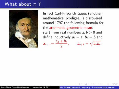
In fact Carl-Friedrich Gauss (anothermathematical prodigee...) discoveredaround 1797 the following formula forthe arithmetic-geometric mean:start from real numbers a, b > 0 anddefine inductively a0 = a, b0 = b and
an+1 =an + bn
2, bn+1 =
√anbn.
Jean-Pierre Demailly (Grenoble I), November 26, 2011 On the computational complexity of mathematical functions
What about π ?
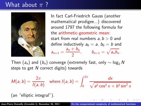
In fact Carl-Friedrich Gauss (anothermathematical prodigee...) discoveredaround 1797 the following formula forthe arithmetic-geometric mean:start from real numbers a, b > 0 anddefine inductively a0 = a, b0 = b and
an+1 =an + bn
2, bn+1 =
√anbn.
Then (an) and (bn) converge (extremely fast, only ∼ log2 Nsteps to get N correct digits) towards
M(a, b) =2π
I (a, b)where I (a, b) =
∫ 2π
0
dx√a2 cos2 x + b2 sin2 x
(an “elliptic integral”).
Jean-Pierre Demailly (Grenoble I), November 26, 2011 On the computational complexity of mathematical functions

The Brent-Salamin formula
Using this and another formula due to Legendre (1752 – 1833),Brent and Salamin found in 1976 a remarkable formula for π.Define
cn =√a2n − b2n
in the arithmetic-geometric sequence. Then
π =4M(1, 1/
√2)2
1−∑+∞
n=1 2n+1c2n
.
Jean-Pierre Demailly (Grenoble I), November 26, 2011 On the computational complexity of mathematical functions
The Brent-Salamin formula
Using this and another formula due to Legendre (1752 – 1833),Brent and Salamin found in 1976 a remarkable formula for π.Define
cn =√a2n − b2n
in the arithmetic-geometric sequence. Then
π =4M(1, 1/
√2)2
1−∑+∞
n=1 2n+1c2n
.
As a consequence, the calculation of N digits of π is also aquasi-linear problem!
Jean-Pierre Demailly (Grenoble I), November 26, 2011 On the computational complexity of mathematical functions

The Brent-Salamin formula
Using this and another formula due to Legendre (1752 – 1833),Brent and Salamin found in 1976 a remarkable formula for π.Define
cn =√a2n − b2n
in the arithmetic-geometric sequence. Then
π =4M(1, 1/
√2)2
1−∑+∞
n=1 2n+1c2n
.
As a consequence, the calculation of N digits of π is also aquasi-linear problem!
This formula has been used several times to break the worldrecord, which seems to be 5 trillions digits since 2010(however, there exist so efficient quadratic complexity formulasthat they are still competitive at that level...)
Jean-Pierre Demailly (Grenoble I), November 26, 2011 On the computational complexity of mathematical functions

Complexity of matrix multiplication
Question. How many steps are necessary to compute theproduct C = AB of two n × n matrices, assuming that eachelementary multiplication or addition takes 1 step?
The standard matrix matrix multiplication algorithm
cik =∑
1≤j≤n
aijbjk , 1 ≤ i , k ≤ n
leads to calculate n2 coefficients, each of which requiresn multiplications and (n − 1) additions, so in totaln2(2n − 1) ∼ 2n3 operations.
However, the size of the data is N = n2, and the generalphilosophy that it should be quasi-linear would suggest analgorithm with complexity less than N1+ε = n2+2ε for every ε.
The fastest known algorithm, due to Coppersmith andWinograd in 1987 has #steps ≤ C n2.38 (quite complicated!)
Jean-Pierre Demailly (Grenoble I), November 26, 2011 On the computational complexity of mathematical functions