8/12/2019 On the Degradation Evolution Equations of Cellulose

http://slidepdf.com/reader/full/on-the-degradation-evolution-equations-of-cellulose 1/20

On the degradation evolution equations of cellulose

H. -Z. Ding Z. D. Wang

Received: 18 January 2007 / Accepted: 9 August 2007 / Published online: 7 October 2007 Springer Science+Business Media B.V. 2007

Abstract Cellulose degradation is usually charac-terized in terms of either the chain scission number orthe scission fraction of cellulose unit as a function of degree of polymerisation (DP) and cellulose degra-dation evolution equation is most commonlydescribed by the well known Ekenstam equations.In this paper we show that cellulose degradation canbe best characterized either in terms of the percentageDP loss or in terms of the percentage tensile strength(TS) loss. We present a new cellulose degradationevolution equation expressed in terms of the percent-age DP loss and apply it for having a quantitativecomparison with six sets of experimental data. Wedevelop a new kinetic equation for the percentage TSloss of cellulose and test it with four sets of experimental data. It turns out that the proposedcellulose degradation evolution equations are able toexplain the real experimental data of differentcellulose materials carried out under a variety of experimental conditions, particularly the prolongedautocatalytic degradation in sealed vessels. We alsodevelop a new method for predicting the degree of degradation of cellulose at ambient conditions bycombining the master equation representing thekinetics of either percentage DP loss or percentage

TS loss at the lowest experimental temperature withArrhenius shift factor function.

Keywords Cellulose Degradation Kinetics Modelling Degree of polymerisation Tensile strength Percentage loss Time–temperature superposition Arrhenius activation energy

Introduction

Cellulose is the main raw material in paper industryand has been widely used as storage paper in booksand documents, and as insulating paper/pressboard inhigh-voltage oil-lled power cables and transformers.In all applications, methods of characterizing cellu-lose degradation and kinetics of cellulose degradationevolution are important, because they not only governthe long-term performance of the paper products butalso ultimately determine the useful life of books,documents, power cables and transformers. Theresearch into the characterization of cellulose degra-dation and the kinetics of cellulose degradationevolution has been a topic for decades and has madeconsiderable progress. Briey, there are three steps inanalysing the kinetics of cellulose degradation. Therst step is to characterize the degradation (i.e., todene the degradation variable) because degradationis not a quantity that can be directly measured. Thesecond step is to describe the evolution equation of

H. -Z. Ding ( & ) Z. D. WangSchool of Electrical and Electronic Engineering, TheUniversity of Manchester, P O Box 88, Sackville Street,Manchester M60 1QD, UK e-mail: hongzhi.ding@manchester.ac.uk

1 3

Cellulose (2008) 15:205–224DOI 10.1007/s10570-007-9166-4

8/12/2019 On the Degradation Evolution Equations of Cellulose

http://slidepdf.com/reader/full/on-the-degradation-evolution-equations-of-cellulose 2/20

degradation variable, which shows how the stressingconditions lead to new degradation in the cellulose.These rst two steps essentially establish the consti-tutive relationship of cellulose with defects. The thirdstep is to use the established constitutive relationshipin the kinetics analysis to predict the degree of

degradation of cellulose at ambient conditions andthe result regarding when the cellulose will fail.

Characterization of cellulose degradation

The characterization of the degradation includeschoosing a proper variable to describe the defectsof the cellulose at the molecular level, and to nd outhow these defects affect the macroscopic behavioursof the cellulose. It is well recognized today that allthermal, hydrolytic, photolytic, photochemical andenzymatic degradation of cellulose are essentiallydue to the scission of polymeric chains (a number of the b-glucosidic bonds being broken). The methodmost commonly used in the literature for character-izing cellulose degradation involves thedetermination of either the Chain Scission Number(CSN) or the Scission Fraction of Cellulose Unit(SFCU) as a function of degree of polymerisation(DP). DP can be determined from the measuredchange of the intrinsic viscosity using the Mark–Houwink equation.

The CSN, which represents the average number of chain scissions per cellulose chain unit during thetime course of degradation, can be calculated usingthe following equation (Hon 1985 ; Moser andDahinden 1987 ; Johansson et al. 2000 ; Bouchardet al. 2006 ; Calvini and Gorassini 2006 )

CSN ¼DP 0

DP 1 ð1Þ

where DP 0 and DP are the degree of polymerisation

before and after the degradation.The SFCU, which represents the ratio of broken

glucose units to the total glucose units of a cellulosechain, can be calculated using the following equation(Hon 1985 ; Chen and Lucia 2003 )

SFCU ¼CSNDP 0

¼ 1DP

1DP 0

ð2Þ

Multiplying the SFCU by a factor of 100 gives thepercentage of the initial bonds that have been broken.

The evolution equations of cellulose degradation

The method most usually used in the literature forfollowing the kinetics of cellulose degradationinvolves the determination of the SFCU as a functionof ageing time ( t ), which assumed a random rst-order

chain scission reaction relationship and showed (Eken-stam 1936 ; Sharples 1971 ; Emsley and Stevens 1994 )

ln 1 1DP 0 ln 1

1DP ¼ kt ð3Þ

If DP 0 and DP are large, then Eq. 3 reduces to

1DP

1DP 0

¼ kt ð4aÞ

This approximation is identical with the expressionobtained by assuming a zero-order reaction. Here k isthe reaction rate constant. Equation 4a is derived fora homogeneous cellulose system. In a heterogeneouscellulose system, the effect of physical structure onhydrolysis degradation has to be taken into account,and the generally approach involves the introductionof the accessible fraction of bonds ( a) in a practicalcellulose system in the determination of the rate of bond scission, then (Sharples 1954 , 1971 )

1DP

1DP 0

¼ akt ð4bÞ

Equations 3 and 4a are named as Ekenstamequations in the literature. The important point inEq. 4a, as was argued by Sharples ( 1971 ), is that arectilinear plot is obtained if the reciprocal of DP isplotted as a function of the time; while the direct plotof DP as a function of time takes the form of arectangular hyperbola which is considered to beobviously misleading. Equation 4a has been widelyused to describe various cellulose degradation such asacidic degradation, light ageing, dry or moist thermalageing in ovens (Krassig and Kitchen 1961 ; Fung1969 ; Shazadeh and Bradbury 1979 ; Zou et al. 1994 ,1996 ; Testa et al. 1994 ). Emsley and Stevens ( 1994 )have shown that Eq. 4a holds for the majority of theaccelerated ageing data available in the literature forthermal degradation of Kraft paper under a variety of experimental conditions (in vacuo, in nitrogen, airand oxygen, and in transformer oil). Zou et al. ( 1996 )have arrived to the same Eq. 4a without anyassumptions about the reaction order, by assuming aconstant bond breaking rate.

206 Cellulose (2008) 15:205–224

1 3

8/12/2019 On the Degradation Evolution Equations of Cellulose

http://slidepdf.com/reader/full/on-the-degradation-evolution-equations-of-cellulose 3/20

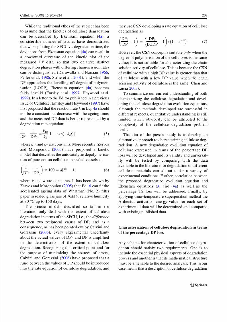
While the traditional ethos of the subject has beento assume that the kinetics of cellulose degradationcan be described by Ekenstam equation ( 4a), aconsiderable number of studies have demonstratedthat when plotting the SFCU vs. degradation time, thedeviations from Ekenstam equation ( 4a) can result in

a downward curvature of the kinetic plot of themeasured DP data, so that two or three distinctdegradation phases with differing chain-scission ratescan be distinguished (Daruwalla and Narsian 1966 ;Feller et al. 1986 ; Strlic et al. 2001 ); and when theDP approaches the levelling-off degree of polymer-isation (LODP), Ekenstam equation ( 4a) becomesfairly invalid (Emsley et al. 1997 ; Heywood et al.1999 ). In a letter to the Editor published in a previousissue of Cellulose, Emsley and Heywood ( 1997 ) haverst proposed that the reaction rate k in Eq. 4a shouldnot be a constant but decrease with the ageing time;and the measured DP data is better represented by adegradation rate equation:

1DP

1DP 0

¼k 10

k 2½1 exp ð k 2 t Þ ð5Þ

where k 10 and k 2 are constants. More recently, Zervosand Moropoulou ( 2005 ) have proposed a kineticmodel that describes the autocatalytic depolymerisa-tion of pure cotton cellulose in sealed vessels as

1DP 1DP 0 100 ¼ a½2kt 1 ð6Þ

where k and a are constants. It has been shown byZervos and Moropoulou ( 2005 ) that Eq. 6 can t theaccelerated ageing data of Whatman (No. 2) lterpaper in sealed glass jars of 76±1% relative humidityat 80 C up to 150 days.

The kinetic models described so far in theliterature, only deal with the extent of cellulosedegradation in terms of the SFCU, i.e., the differencebetween two reciprocal values of DP, and as aconsequence, as has been pointed out by Calvini andGorassini ( 2006 ), every experimental uncertaintyabout the actual values of DP 0 and DP is ampliedin the determination of the extent of cellulosedegradation. Recognizing this critical point and forthe purpose of minimizing the sources of errors,Calvini and Gorassini ( 2006 ) have proposed that aratio between the values of DP should be introducedinto the rate equation of cellulose degradation, and

they use CSN developing a rate equation of cellulosedegradation as

DP 0

DP 1 ¼

DP0

LODP1 1 e kt ð7Þ

However, the CSN concept is suitable only when thedegree of polymerisation of the celluloses is the samevalue; it is not suitable for characterizing the chainscission activity of cellulose. This is because the CSNof cellulose with a high DP value is greater than thatof cellulose with a low DP value when the chainscission activity of cellulose is the same (Chen andLucia 2003 ).

To summarize our current understanding of bothcharacterizing the cellulose degradation and devel-oping the cellulose degradation evolution equations,although the methods developed are successful indifferent respects, quantitative understanding is stilllimited, which obviously can be attributed to thecomplexity of the cellulose degradation problemitself.

The aim of the present study is to develop analternative approach to characterizing cellulose deg-radation. A new degradation evolution equation of cellulose expressed in terms of the percentage DPloss will be developed and its validity and universal-ity will be tested by comparing with the dataavailable in the literature for degradation of differentcellulose materials carried out under a variety of experimental conditions. Further, correlation betweenthe proposed degradation evolution equation andEkenstam equations ( 3) and (4a) as well as thepercentage TS loss will be addressed. Finally, byapplying time–temperature superposition method theArrhenius activation energy value for each set of experimental data will be determined and comparedwith existing published data.

Characterization of cellulose degradation in termsof the percentage DP loss

Any scheme for characterization of cellulose degra-dation should satisfy two requirements. One is toinclude the essential physical aspects of degradationprocess and another is that its mathematical structuremust be amenable to the desired analysis. This in ourcase means that a description of cellulose degradation

Cellulose (2008) 15:205–224 207

1 3

8/12/2019 On the Degradation Evolution Equations of Cellulose

http://slidepdf.com/reader/full/on-the-degradation-evolution-equations-of-cellulose 4/20

that produces consistent relationships between deg-radation and material response and allowsrepresentation of degradation evolution rates isneeded.

The idea to characterize cellulose degradation interms of the percentage DP loss is based on the

essential degradation mechanism in cellulose. Cellu-lose consists of linear, polymeric chains of cyclic, b -D-glucopyranosyl units, and the number of such unitsper chain is called the degree of polymerisation. Thechains of cellulose associate in both crystalline andamorphous regions to form micro-brils, and nallyform bres. Thus, the depolymerisation and theincrease in the number of chain scissions is theessential mechanism of cellulose degradation, and theirreversibility is caused by the energy dissipationassociated with acid-hydrolysis, oxidation and pyro-lysis. A basic unit or entity of cellulose degradationprocess is a chain scission. In view of the fact thatthere is a well-documented connection between thedecrease of DP and the severity of cellulose degra-dation, without loss of generality, we can introduce acontinuous scalar variable d and call it ‘‘percentageretention of DP’’:

d ¼ DPDP 0

ð8Þ

where DP 0 denotes the initial degree of polymerisa-

tion and DP the real degree of polymerisation,decreased as a result of deterioration due to degra-dation of cellulose. The variable d starts from d = 1and decreases to d = 0 (or LODP results in a certainvalue dc ); the last value denotes total failure.

Degradation variable of cellulose can then bedened in terms of the percentage DP loss as

x DP 1 d ¼ 1 DPDP 0

ð9Þ

where x DP is the accumulated DP loss of cellulose.

Using Eq. 9 the extent of cellulose degradation canbe quantied by measuring the DP of the cellulose; itstarts from x DP = 0, which corresponds to virgincellulose and the 100% retention of DP, ending withx DP = 1, which corresponds to total failure of cellulose. It should be noted here that for the failurestate of cellulose, the accumulated degradation maybe not necessary to reach the theoretical maximalvalue of x DP , namely x DP = 1, but a certain smallervalue of x DPcr depending on specic experimental

conditions. It is generally accepted that when the DPhas decreased to an average DP of about 200 thecellulose paper will lose all its mechanical strength; if DP 0 = 1,200, then dc = 0.1667, and the accumulateddegradation critical value x DPcr = 0.8333.

As a method of expressing the rate of cellulose

degradation, the percentage DP loss is calculatedfrom the ratio between the values of DP. With thismethod, the expression of degradation is not onlymathematically convenient but also more accuratethan the usual SFCU or CSN method. Further,according to the present denition of cellulosedegradation by Eq. 9, the physical meaning of thedegradation variable x DP is the extent of progressiontowards a maximum tolerable value, and the nature of ageing in cellulose is that degradation accumulatesgradually in the course of stressing time and failure

occurs when these reaches a critical level.

Degradation evolution equation of celluloseexpressed in terms of the percentage DP loss

Degradation evolution equation of cellulose at amolecular level

We begin our theoretical analysis by discussing chainscission degradation of polymer at a molecular level.Experimental and analytical investigations havedemonstrated that degradation of cellulose is due tothermally activated polymeric chain scissions. Thus,chemical reaction rate theory has been widelyemployed to model cellulose degradation processes.The exact mechanisms that lead to failure of cellulosematerials, however, are not known a priori. As aconsequence, various hypotheses have to be proposedand sophisticated models with unknown parametershave to be developed. Whatever the exact mecha-nisms may be, it appears that degradation evolutionequations based on chemical reaction rate theorydescribe the kinetics of cellulose degradation reason-ably well, although certain modications may benecessary to account for experimental observations.On the other hand, there is now a great deal of experimental evidence in polymers that chain scis-sion occurs during the degradation and failure of polymers and particularly, although the concentrationof chain scissions is a time function of the degrada-tion, the total accumulation of chain scissions at

208 Cellulose (2008) 15:205–224

1 3

8/12/2019 On the Degradation Evolution Equations of Cellulose

http://slidepdf.com/reader/full/on-the-degradation-evolution-equations-of-cellulose 5/20

failure for a given polymer is, to a good approxima-tion, independent of the loading conditions(Kukensko and Tamuzs 1981 ). The chain scissionconcentration N of a polymer thereby represents alogical scalar parameter with which to characterizedegradation within the material.

In order to quantitatively model the kinetic processof cellulose degradation, it is assumed that on themolecular level degradation is the result of chainscission and, there exists, at time equals zero, acertain number of potentially weak bonds denoted by N T , which will be available for the degradation.Therefore, according to chemical reaction rate theory,the rst-order reaction kinetics of degradation can bewritten as

d N

dt

¼ k N T N ð Þ; N ðt ¼ 0Þ ¼ 0 ð10Þ

The above differential equation relates the time rateof change of the accumulated chain scission concen-tration to the number of weak bonds available timesthe chain scission reaction rate. Here k is the chainscission reaction rate constant, and the initial condi-tion implies that the material has undergone noprevious chain scission.

The general solution to Eq. 10 is given by

N ðt Þ ¼

Z

t

0

N Tk ð xÞexp

Z

t

x

k ð yÞd y

d x ð11Þ

But for a constant reaction rate k the exact solutionmay be written in the form

N ¼ N Tð1 e kt Þ ð12Þ

If N N T ; then

N ffi N Tkt ð13Þ

This expression is identical with a zero-order approx-imation solution of Eq. 10. As was noticed by Calvini(2005 ), it is not difcult to verify that Ekenstamequations ( 3) and (4a) can be derived from the aboveEqs. 12 and 13, respectively, if we consider that N = SFCU = (1/DP–1/DP 0 ) and N T = (1–1/DP 0 ).Also, it is easy to verify that Eq. 7 can be derivedfrom Eq. 12, if we consider that N = CSN = (DP 0 / DP–1) and N T = (DP 0 /LODP–1) (Calvini and Goras-sini 2006 ).

Bear in mind that the chain scission concentrationin polymers at failure N F is approximately a constant.

We can therefore introduce a normalized chainscission degradation variable of the form

nðt Þ N ðt Þ N F

ð14Þ

Based on this denition, we can quantify the degree of

degradation at a molecular level as follows: (1) n = 0corresponds to no degradation; (2) n = 1 correspondsto failure; and (3) 0 \ n \ 1 implies that the materialhas undergone some permanent chain scission degra-dation. In terms of the normalized chain scissiondegradation variable, Eq. 10 becomes

dndt

¼ k ðn nÞ; nðt ¼ 0Þ ¼0 ð15Þ

where n* = N T / N F represents the capacity of the chainscission reservoir. For a constant reaction rate k the

time-evolution equation of the normalized chainscission degradation variable n(t ) obeys

n ¼ n ð1 e kt Þ ð16Þ

Equations 15 and 16 stand for the evolution rules of cellulose degradation at a molecular level. We notethat expressions similar to Eqs. 15 and 16 have beenreported in the literature for describing the kinetics of mechanochemical scission of the main chains of polymer molecules (Zhurkov and Korsukov 1974 ;Petrov 1984 ; Hansen and Baker-Jarvis 1990 ).

A new degradation evolution equation forcellulose

In view of the similarity between two denitions of degradation state variable, n at a molecular level andx DP at a macroscopic level, without loss of gener-ality, we can assume that the differential equationgoverning the time dependence of x DP at a macro-scopic level has exactly the same form as that of n ata molecular level. Thus, analogous to Eq. 15, thedegradation evolution equation governing the timedependence of x DP for cellulose assumes the form

dx DP

dt ¼ k DP ðx DP x DP Þ; x DP ðt ¼ 0Þ ¼0 ð17Þ

Equation 17 relates the time rate of change of theaccumulated DP degradation of cellulose, d x DP /dt , tothe residual DP level available for the degradation,

Cellulose (2008) 15:205–224 209

1 3

8/12/2019 On the Degradation Evolution Equations of Cellulose

http://slidepdf.com/reader/full/on-the-degradation-evolution-equations-of-cellulose 6/20

8/12/2019 On the Degradation Evolution Equations of Cellulose

http://slidepdf.com/reader/full/on-the-degradation-evolution-equations-of-cellulose 7/20

Eq. 18. The paper ageing data are originally reportedby Soares et al. ( 2001 ) in the form of DP vs. ageingtime. The paper samples were made by Mukyuo inSweden for transformer grade (774 kg/m 3 , DP 0 =1,183). Ageing experiments were conducted in air

for up to 140 h in the temperature range 70–120 C.The estimated values of the parameters for each curvetting are given in Table 2, with the values of all theregression coefcients R2

[ 0.996.

Ageing data of Kraft paper in transformer mineraloil at high water/oxygen level

Figure 3 shows plots of the degree of degradationchange during thermal ageing of Kraft pulp paper(774 kg/m 3 , DP 0 = 1,183) in mineral transformer oil,together with the corresponding predictions usingEq. 18. The ageing data are originally reported by

Soares et al. ( 2001 ) in the form of DP vs. ageingtime. The transformer oil for ageing experiments wasTexaco grade DNC 3230 standard mineral oil, usedas received. Ageing experiments were conducted intransformer oil for up to 3,500 h in the temperaturerange 65–120 C. Air was not excluded during thevarying period of ageing. The estimated values of theparameters for each curve tting are given in Table 3,with the values of all the regression coefcients R2

[ 0.974.

Ageing data of Kraft paper in transformer mineraloil at low water/oxygen level

Figure 4 shows plots of the degree of degradationchange during thermal ageing of Kraft insulationpaper (DP 0 = 1,250) in mineral transformer oil atlow-water/low oxygen levels, together with thecorresponding predictions using Eq. 18. The DP dataare originally reported by Emsley et al. ( 2000a ).

Before starting the ageing experiments, the Kraftpaper (from Tullis Russell) samples were dried in apot overnight at 115 C under vacuum, and thetransformer oil was degassed at 60 C overnight in avacuum. The water in the paper was measured to beless than 0.1% and the oxygen in the oil less than400 ppm. Ageing experiments were conducted indegassed transformer oil for up to 12,000 h in thetemperature range 120–160 C. The estimated valuesof the parameters for each curve tting are given in

0 20 40 60 80 100 120 1400.0

0.2

0.4

0.6

0.8

1.0 data of 70 oC data of 80 oC data of 90 oC data of105 oC data of120 oC fitting curvesby Eq.(18) fitting curvesby Eq.(21)

, n o i t a

d a r

g e d f o e e r g e

D

ω P D

Ageing time (hours)

Fig. 2 Degree of degradation change during thermal ageing of Kraft paper in air; experimental data of DP are after Soareset al. ( 2001 )

Table 2 Calculated parameters for tting equations ( 18) and(21) to the data in Fig. 2

T ( C) Equation 18 Equation 21

x DP* k DP (1/h) R2 k ( · 10 –6 , 1/h) R2

70 0.1952 0.0227 0.9968 1.9189 0.8613

80 0.2796 0.0199 0.9987 2.8741 0.9212

90 0.4149 0.0248 0.9969 5.7227 0.9260

105 0.4357 0.0294 0.9995 6.7625 0.9084

120 0.5015 0.0351 0.9959 9.5182 0.9131

0 500 1000 1500 2000 2500 3000 35000.0

0.2

0.4

0.6

0.8

1.0

, n o i t a

d a r g e d f o e e r g e

D

ω P D

Ageing time (hours)

data of 65 oC data of 80 oC data of 120 oC fitting curves by Eq.(18) fitting curves by Eq.(21)

Fig. 3 Degree of degradation change during thermal ageing of Kraft paper in transformer mineral oil; experimental data of DPare after Soares et al. ( 2001 )

Cellulose (2008) 15:205–224 211

1 3

8/12/2019 On the Degradation Evolution Equations of Cellulose

http://slidepdf.com/reader/full/on-the-degradation-evolution-equations-of-cellulose 8/20

Table 4, and the minimum value of the regressioncoefcient for the data at 120 C is R2 = 0.9167.

Ageing data of pure cotton cellulose in sealedvessels at 80 C and 75% RH

Figure 5 shows plots of the degree of polymerisationand the degree of degradation change during thermalageing of pure cotton cellulose in sealed vessels,together with the corresponding predictions usingEq. 18. Application of Eq. 6 has also been includedin Fig. 5 for comparison. The experimental data are

originally reported by Zervos and Moropoulou ( 2005 )in the form of viscosity-average DP v vs. ageing time.The pure cotton cellulose samples were Whatman(No. 2) lter papers ( DP v0 ¼ 1 ; 810 ; cut in test-stripsof 15 mm width). Ageing experiments were con-ducted in sealed glass jars of 76±1% relativehumidity at 80 C up to 240 days. The estimatedvalues of the parameters for curve tting are given inTable 5, and the value of the regression coefcient is R2 = 0.9954.

Ageing data of thermally upgraded Kraft paper insealed vessels with mineral transformer oil andnatural ester respectively

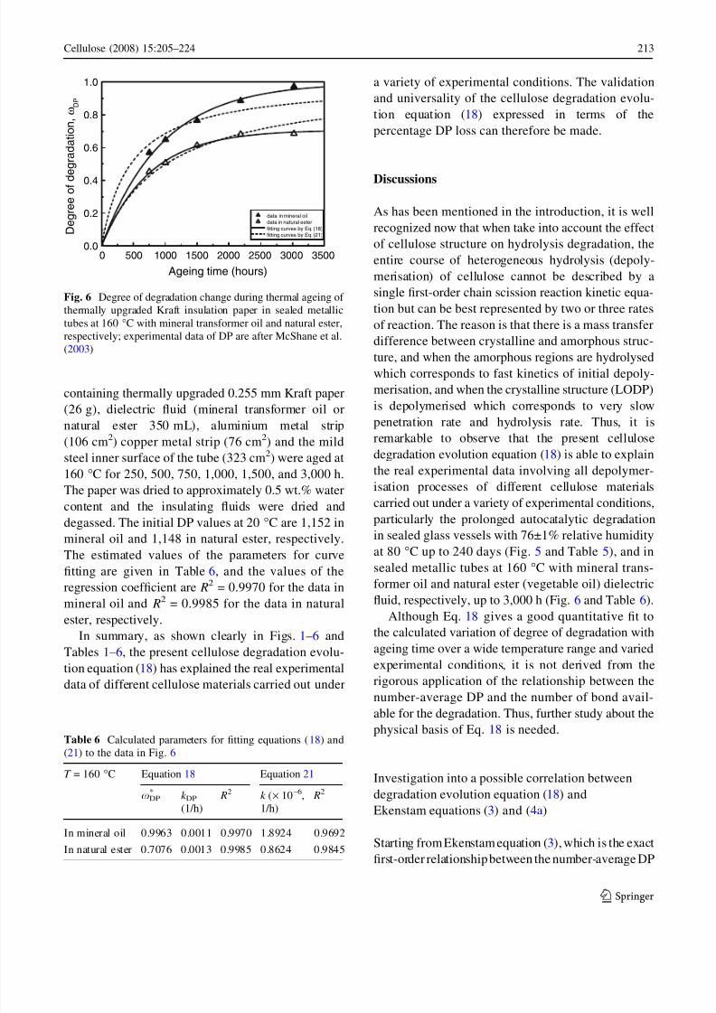
Figure 6 shows plots of the degree of degradationchange during thermal ageing of thermally upgradedKraft insulation paper in sealed metallic tubes at160 C with mineral transformer oil and natural ester(vegetable oil) dielectric uid, respectively, togetherwith the corresponding predictions using Eq. 18. Theexperimental data of DP are originally reported byMcShane et al. ( 2003 ). Sealed steel ageing vesselswith a nitrogen headspace of 17% by volume

Table 3 Calculated parameters for tting equations ( 18) and(21) to the data in Fig. 3

T ( C) Equation 18 Equation 21

x DP* k DP (1/h) R2 k ( · 10 –6 , 1/h) R2

65 0.3032 0.0005 0.9740 0.1014 0.9351

80 0.6983 0.0018 0.9931 1.0059 0.9377120 0.7554 0.0032 0.9971 1.8681 0.8972

0 2000 4000 6000 8000 10000 120000.0

0.2

0.4

0.6

0.8

1.0

g e

D

r

o e e

f

g e

d

t a

d a r

, n o i

ω P D

Ageing time (hours)

data of 120 oC data of 140 oC data of 160 oCfitting curves by Eq. (18)fitting curves by Eq. (21)

Fig. 4 Degree of degradation change during thermal ageing of Kraft paper in transformer mineral oil at low-water/low oxygenlevels; experimental data of DP are after Emsley et al. ( 2000a )

0 40 80 120 160 200 240 2800.0

0.2

0.4

0.6

0.8

1.0ω

DP data at 80 oC fitting curve by Eq. (18) fitting curve by Eq. (21)

, n o i t a

d a r g e

d f o

e e r g e

D

ω P D

Ageing time (days)

0.0

0.2

0.4

0.6

0.8

1.0

DP dataat 80 oC fittingcurve byEq. (6)

P D / 1 - P D / 1 (

0

0 0 1 x )

Fig. 5 Degree of degradation change during thermal ageing of pure cotton cellulose in sealed vessels; experimental data of DPare after Zervos and Moropoulou ( 2005 )

Table 4 Calculated parameters for tting equations ( 18) and(21) to the data in Fig. 4

T ( C) Equation 18 Equation 21

x DP* k DP (1/h) R2 k ( · 10 –6 , 1/h) R2

120 0.6600 0.0008 0.9167 0.3200 0.8199

140 0.9000 0.0018 0.9719 2.0080 0.9865

160 0.9500 0.0063 0.9796 8.0000 0.9673

Table 5 Calculated parameters for tting equations ( 18) and(21) to the data in Fig. 5

T ( C) Equation 18 Equation 21

x DP* k DP

(1/day) R2 k ( · 10 –5 ,

1/day) R2

80 1.0100 0.0137 0.9954 1.5503 0.9458

212 Cellulose (2008) 15:205–224

1 3

8/12/2019 On the Degradation Evolution Equations of Cellulose

http://slidepdf.com/reader/full/on-the-degradation-evolution-equations-of-cellulose 9/20

containing thermally upgraded 0.255 mm Kraft paper(26 g), dielectric uid (mineral transformer oil ornatural ester 350 mL), aluminium metal strip(106 cm 2 ) copper metal strip (76 cm 2 ) and the mildsteel inner surface of the tube (323 cm 2 ) were aged at160 C for 250, 500, 750, 1,000, 1,500, and 3,000 h.The paper was dried to approximately 0.5 wt.% watercontent and the insulating uids were dried anddegassed. The initial DP values at 20 C are 1,152 inmineral oil and 1,148 in natural ester, respectively.The estimated values of the parameters for curvetting are given in Table 6, and the values of theregression coefcient are R2 = 0.9970 for the data inmineral oil and R2 = 0.9985 for the data in naturalester, respectively.

In summary, as shown clearly in Figs. 1–6 andTables 1–6, the present cellulose degradation evolu-tion equation ( 18) has explained the real experimentaldata of different cellulose materials carried out under

a variety of experimental conditions. The validationand universality of the cellulose degradation evolu-tion equation ( 18) expressed in terms of thepercentage DP loss can therefore be made.

Discussions

As has been mentioned in the introduction, it is wellrecognized now that when take into account the effectof cellulose structure on hydrolysis degradation, theentire course of heterogeneous hydrolysis (depoly-merisation) of cellulose cannot be described by asingle rst-order chain scission reaction kinetic equa-tion but can be best represented by two or three ratesof reaction. The reason is that there is a mass transferdifference between crystalline and amorphous struc-ture, and when the amorphous regions are hydrolysedwhich corresponds to fast kinetics of initial depoly-merisation, and when the crystalline structure (LODP)is depolymerised which corresponds to very slowpenetration rate and hydrolysis rate. Thus, it isremarkable to observe that the present cellulosedegradation evolution equation ( 18) is able to explainthe real experimental data involving all depolymer-isation processes of different cellulose materialscarried out under a variety of experimental conditions,particularly the prolonged autocatalytic degradationin sealed glass vessels with 76±1% relative humidityat 80 C up to 240 days (Fig. 5 and Table 5), and insealed metallic tubes at 160 C with mineral trans-former oil and natural ester (vegetable oil) dielectricuid, respectively, up to 3,000 h (Fig. 6 and Table 6).

Although Eq. 18 gives a good quantitative t tothe calculated variation of degree of degradation withageing time over a wide temperature range and variedexperimental conditions, it is not derived from therigorous application of the relationship between thenumber-average DP and the number of bond avail-able for the degradation. Thus, further study about thephysical basis of Eq. 18 is needed.

Investigation into a possible correlation betweendegradation evolution equation ( 18) andEkenstam equations ( 3) and (4a)

Starting fromEkenstam equation ( 3), which is the exactrst-order relationshipbetween the number-average DP

0 500 1000 1500 2000 2500 3000 35000.0

0.2

0.4

0.6

0.8

1.0

, n o i t a

d a r g e

d f o e e r g e

D

ω P D

Ageing time (hours)

data in mineral oildata in natural esterfitting curves by Eq. (18)fitting curves by Eq. (21)

Fig. 6 Degree of degradation change during thermal ageing of thermally upgraded Kraft insulation paper in sealed metallictubes at 160 C with mineral transformer oil and natural ester,respectively; experimental data of DP are after McShane et al.(2003 )

Table 6 Calculated parameters for tting equations ( 18) and(21) to the data in Fig. 6

T = 160 C Equation 18 Equation 21

x DP* k DP

(1/h) R2 k ( · 10 –6 ,

1/h) R2

In mineral oil 0.9963 0.0011 0.9970 1.8924 0.9692

In natural ester 0.7076 0.0013 0.9985 0.8624 0.9845

Cellulose (2008) 15:205–224 213

1 3

8/12/2019 On the Degradation Evolution Equations of Cellulose

http://slidepdf.com/reader/full/on-the-degradation-evolution-equations-of-cellulose 10/20

and the number of bond available for the degradation,simply by making a rearrangement in Eq. 3 it is notdifcult to have the following form

1 DPDP 0

¼ ðDP 0 1Þ

1 þ ð DP 0 1Þð1 e kt Þð1 e kt Þ

ð19ÞWe call Eq. 19 a modied Ekenstam equation, whichis exactly identical to Eq. 3.

It is interesting to observe that the new cellulosedegradation evolution equation ( 18) looks exactly thesame as Eq. 19 if we can assume that k DP is equal to k and

x DP ðDP 0 1Þ

1 þ ð DP 0 1Þð1 e kt Þ ð20Þ

It is important to realize that x DP* in Eq. 18 is

independent of time but according to Eq. 20 is afunction of degradation time. However, this obser-vation has interesting potential for further study.According to Eq. 20, the minima of x DP

* is (1–1/ DP 0 ); i.e., we will always have x DP

*[ 1–1/DP 0 .

Applying this result for six sets of experimental dataplotted in Figs. 1–6 and it is easy to show thatx DP

*[ 1–1/DP 0 means x DP

*[ 0.9990 for all exper-

imental data. However, the preceding analysis of theexperimental data according to Eq. 18 has resultedin the evaluation of x DP

* , as shown in Tables 1–6.Nearly all values of x DP

* in Tables 1–6 are smallerthan (1–1/DP 0 ) except the value x DP

* = 1.01 inTable 5. The larger value of x DP

* = 1.01 in Table 5was attributed obviously to the fact that thedegradation process was a prolonged autocatalyticreaction process, which in our opinion, means apromoted number of effective chains taking part inscission so that the required chain scission numberat failure under such an autocatalytic reactioncondition is less than the available number of

potentially weak bonds.Due to its complex expression, the modiedEkenstam equation ( 19) is mathematically not con-venient to be utilized in explaining real experimentaldata. When both DP 0 and DP are large (i.e., the extentof DP degradation reaction is small), using theapproximation as same as in the Ekenstam’sapproaches in obtaining Eq. 4a, the modied Eken-stam equation ( 19) can be simplied as

1 DPDP 0

¼ DP0kt 1 þ DP 0kt

ð21Þ

This equation is exactly identical to the widely usedEkenstam equation ( 4a). Application of Eq. 21 andcomparison with real experimental results of cellu-lose degradation have been included in Figs. 1–6 andTables 1–6.

To this end, a simple but far-reaching statementcan now be made. In short, some experimental datacan be described equally well with both Eqs. 18 and21. However, this does not mean that all data that canbe described by Eq. 18 can also be described byEq. 21. For example, in Figs. 2, 5, such experimentaldata can hardly be described by Eq. 21. Bear also inmind that the constraint of x DP

*[ 1–1/DP 0 according

to Eq. 20 does not apply for Eq. 18. In these sensesEkenstam equations ( 3) and (4a) or (19) and (21) canbe considered (roughly) as a special case of Eq. 18.

Investigation into a possible correlation betweendegradation evolution equation ( 18) and tensilestrength

No attempt is made, in this paper, to include adetailed study on the possible correlation between thekinetics of cellulose degradation and the changes in a

wide range of macroscopic properties. In whatfollows, we show how the concept of degradationaccumulation in terms of the percentage DP lossdeveloped in the present study can be used to derive akinetic equation for loss of tensile strength of cellulose and paper.

Bear in mind that the main feature of tensilestrength loss of cellulose and paper is the successivechain scission in cellulose bre. Accelerated ageingtest of pure cellulose papers in air (Zou et al. 1994 )and Kraft papers in transformer oil (Emsley et al.

2000b ) have demonstrated that the loss of tensilestrength during the degradation is due to a decrease inbre strength and not bond strength loss; and thedecrease in bre strength is due to depolymerisationof the cellulose caused by acid-catalysed hydrolysis.Hence, similar to the denition of degradation of cellulose in terms of the percentage DP loss by Eq. 9,we can introduce a new degradation variable x TS

which is dened as the percentage TS loss, from an

214 Cellulose (2008) 15:205–224

1 3

8/12/2019 On the Degradation Evolution Equations of Cellulose

http://slidepdf.com/reader/full/on-the-degradation-evolution-equations-of-cellulose 11/20

initial value of the tensile strength TS 0 to the currenttensile strength TS:

x TS 1 TSTS 0

ð22Þ

Using the similar arguments as described in the

previous section in deriving the generalized cellulosedegradation equation ( 18), a new kinetic equation forloss of tensile strength of cellulose, which is analo-gous to Eq. 18, can be obtained as

x TS 1 TSTS 0

¼ x TS ð1 e k TS t Þ ð23Þ

where k TS is the TS degradation rate constant and x TS*

is the capacity of the TS degradation reservoir. Thevalue of x TS

* can be determined by introducing theconstraint condition: x TS (t = t f ) = 1, t f is the time to

failure.Let us now attempt to reconcile the above Eq. 23

with four specic experimental data reported in theliterature. Figure 7 shows the zero-span tensilestrength loss of Whatman lter paper (II) and cottonlinter sheets during thermal ageing at 90 C andrelative humidity 80% and corresponding regressionanalysis t of Eq. 23. The ageing data are originallyreported by Zou et al. ( 1994 ). The values of theparameters for each curve tting are given in Table 7,and the values of the regression coefcient are

R2

= 0.9767 for the data of Whatman lter paperand R2 = 0.9832 for the data of cotton linter sheets,respectively.

Figure 8 shows plots of the tensile strength loss vs.accelerated ageing time for results of thermallyupgraded insulation paper aged in closed, air-tightsystem with mineral transformer oil at 120, 135 and150 C, together with the corresponding predictionsusing Eq. 23. The ageing data of TS are originallyreported by Gasser et al. ( 1999 ). As reported, the oilwas dried and degassed mineral oil Shell Diala D;and copper and iron were loaded on to the frames ascatalysts. The weight ratio of Oil:Paper:Cu:Fe in theageing experiments was 100:2.5:0.45:0.33. The val-ues of the parameters for each curve tting are givenin Table 8, with the minimum value of all theregression coefcients is R2 = 0.9869.

Figure 9 shows plots of the tensile strength loss vs.accelerated ageing time for results of thermallyupgraded Kraft paper sealed tube aged at 160 C inmineral transformer oil and natural ester obtainedfrom McShane et al. ( 2003 ) along with the corre-sponding regression analysis t made with Eq. 23.The values of the parameters for each curve tting are

0 5 10 15 20 250.0

0.2

0.4

0.6

0.8

1.0

, n o i t a

d a r g e

d f

o e e r g e

D

ω S T

Ageing time (days)

Data of Cotton linter sheets Data of Whatman filter paperfitting curves by Eq. (23)fitting curves by Eq. (25)

Fig. 7 Zero-span tensile strength loss of Whatman lter paper(II) and cotton linter sheets during thermal ageing at 90 C andrelative humidity 80%; experimental data of TS are after Zouet al. ( 1994 )

Table 7 Calculated parameters for tting equations ( 23) and(25) to the data in Fig. 7

90 C, 80% RH Equation 23 Equation 25

x TS* k TS

(1/day) R2 C TS

(1/day) R2

Cotton lintersheets

0.3693 0.0851 0.9832 0.0214 0.9205

Whatman lterpaper (II)

0.6983 0.1214 0.9767 0.0644 0.9372

0 50 100 150 200 250 300 350 4000.0

0.2

0.4

0.6

0.8

1.0

, n o i t a

d a r g e d f o e e r g e

D

ω S T

Ageing time (days)

Data of 120 oC Data of 130 oC Data of 150 oC fitting curves byEq. (23) fitting curves byEq. (25)

Fig. 8 Tensile strength loss of thermally upgraded insulationpaper aged in mineral transformer oil; experimental data of TSare after Gasser et al. ( 1999 )

Cellulose (2008) 15:205–224 215

1 3

8/12/2019 On the Degradation Evolution Equations of Cellulose

http://slidepdf.com/reader/full/on-the-degradation-evolution-equations-of-cellulose 12/20

given in Table 9, and the values of the regressioncoefcient are R2 = 0.9786 for the data in mineral oiland R2 = 0.9613 for the data in natural ester,respectively.

Figure 10 shows plots of the tensile strength lossvs. accelerated ageing time for results of Kraftinsulation paper aged in dried and degassed trans-former oil (Shell Diala B) in the temperature range129–166 C under vacuum, together with the corre-sponding predictions using Eq. 23. The TS data are

originally reported by Hill et al. ( 1995 ) in the form of TS vs. ageing time. The values of the parameters foreach curve tting are given in Table 10, with theminimum value of all the regression coefcients is R2 = 0.9827.

In summary, as shown clearly in Figs. 7–10 andTables 7–10, the good agreement between the pre-dictions by Eq. 23 expressed in terms of thepercentage TS loss and experimental data appearsto be justied in principle even with limited data.

It is interesting to note that the good agreementobserved on Figs. 7–10 was obtained according toEq. 23 with two tting parameters, that is much lessthan in Emsley and Heywood model ( 1997 ) whichhave ve tting parameters. Starting from Eq. 5,Emsley and Heywood ( 1997 ) had studied thecorrelation between the kinetics of cellulose degra-dation and the tensile strength loss, and derived arelationship for loss of tensile strength with time asfollows

Table 8 Calculated parameters for tting equations ( 23) and(25) to the data in Fig. 8

T ( C) Equation 23 Equation 25

x TS* k TS (1/day) R2 C TS (1/day) R2

120 0.5869 0.0028 0.9958 0.0014 0.9873

130 0.9430 0.0034 0.9869 0.0031 0.9868150 0.5761 0.0335 0.9978 0.0115 0.9119

0 500 1000 1500 2000 2500 3000 35000.0

0.2

0.4

0.6

0.8

1.0

D

, n o i t a

d a r g e

d f o

e e r g e

ω S T

Ageing time (hours)

TS data in mineral oilTS data in natural esterfitting curves by Eq. (23)fitting curves by Eq. (25)

Fig. 9 Tensile strength loss of thermally upgraded Kraftinsulation paper in sealed metallic tubes at 160 C withmineral transformer oil and natural ester respectively; exper-imental data of TS are after McShane et al. ( 2003 )

Table 9 Calculated parameters for tting equations ( 23) and(25) to the data in Fig. 9

160 C Equation 23 Equation 25

x TS* k TS (1/h) R2 C TS (1/h) R2

In naturalester

0.3990 0.0008 0.9613 0.0002 0.8460

In mineraloil

4.7800 0.0001 0.9786 0.0006 0.9027

0 5 10 15 20 25 300.0

0.2

0.4

0.6

0.8

1.0

D

, n o i t a

d a r g e

d f o e e r g e

ω S T

Ageing time (days)

Data of 129 oC Data of 138 oC Data of 153 oC Data of 166 oCfitting curves by Eq. (23)fitting curves by Eq. (25)

Fig. 10 Tensile strength loss of Kraft insulation paper aged indried and degassed transformer oil; experimental data of TS areafter Hill et al. ( 1995 )

Table 10 Calculated parameters for tting equations ( 23) and(25) to the data in Fig. 10

T ( C) Equation 23 Equation 25

x TS* k TS

(1/day) R2 C TS

(1/day) R2

129 1.0000 0.0153 0.9827 0.0153 0.9827

138 0.6419 0.0396 0.9913 0.0211 0.9856

153 0.9537 0.0526 0.9972 0.0490 0.9971

166 0.8030 0.1987 0.9962 0.1118 0.9434

216 Cellulose (2008) 15:205–224

1 3

8/12/2019 On the Degradation Evolution Equations of Cellulose

http://slidepdf.com/reader/full/on-the-degradation-evolution-equations-of-cellulose 13/20

TS TS 0 ¼ K 1e k 2 t þ K 2ðlnðek 2 t K 3ÞÞ K 4 ð24Þ

where k 2 , K 1 , K 2 , K 3 and K 4 are constants, and TS 0 isthe tensile strength value at the initial. Note thatEq. 24 was initially developed using air-aged resultsof Kraft insulation paper (Emsley et al. 1997 ) andhad been applied equally to mineral transformer oil-aged Kraft paper (Emsley et al. 2000b ). One dif-culty with the Emsley and Heywood model Eq. 24 tomake practical estimates from limited ageing exper-imental data is the relative complexity of tensilestrength loss with time.

It is also noted that one of the earliest kineticmodels for loss of tensile strength of paper in theliterature was formulated empirically by researchersat Weidmann 1 and reported in their Transformer-board II (Moser and Dahinden 1987 ; also Gasseret al. 1999 ) as follows:

TS ¼ TS 0e C TS t ð25a Þ

where TS 0 and TS are the tensile strength valuesbefore and after an ageing time, respectively, C TS isthe coefcient of ageing rate by 1/days and t is theduration of ageing by days. This kinetic expressionhas the advantage of requiring fewer data points, butcan only be applied to long-term ageing of paper. Hillet al. (1995 ) have derived the same Eq. 25a with

assumptions that the chain scission reaction can berepresented by a zero-order kinetic but the relation-ship between the tensile strength and bond scission isrst-order kinetic model. According to Hill et al.(1995 ), the parameter C TS in Eq. 25a is a zero-orderrate constant for chain scission. Simply by making arearrangement in Eq. 25a it is easy to have thefollowing form

1 TSTS 0

¼ 1 e C TS t ð25b Þ

This expression is exactly a special case of Eq. 23when set parameter x TS

* = 1. Application of equation(25b ) and quantitative comparison with four sets of experimental data have been included in Figs. 7–10and Tables 7–10, which show that Eq. 25b can alsot the data approximately, but the values of theregression coefcient R2 are always smaller thanthose of new kinetic equation ( 23).

It is interesting to observe that nearly all valuesof x TS

* in Tables 7–10 are, similar to the values of

x DP* in Tables 1–6, smaller than (1–1/DP 0 ) except the

value x TS* = 4.78 in Table 9 and x TS

* = 1 inTable 10. The larger value of x TS

* = 4.78 for thermalageing of thermally upgraded Kraft insulation paperin sealed metallic tubes in Table 9 was againattributed obviously to the fact that the degradation

process was a prolonged autocatalytic reaction pro-cess particularly with the presence of metalliccatalysts. This is essentially because the requiredchain scission number at failure under such aprolonged autocatalytic reaction condition is wellless than the available number of potentially weak bonds. As a matter of fact, the effect of metals oncellulose degradation is well recognized in theliterature (Williams et al. 1977 ; McCrady 1996 andreferences; Baran ´ ski et al. 2006 ), and it is also wellknown that both hydrolytic and oxidative processesmay occur simultaneously in the ageing of paper(Arney and Noval 1982 ; Margutti et al. 2001 ). Withthese in mind, it is reasonably to believe thatdegradation of thermally upgraded Kraft insulationpaper in sealed metallic tubes in Fig. 9 and Table 9 iscaused by at least two processes—acid-catalysedhydrolysis and metal-catalysed oxidation. From thispoint, it is remarkable that Eq. 23 holds even in themixed hydrolytic and oxidative processes of cellulosedegradation.

We point out that the similarity of mathematicalexpression between Eqs. 23 and 18 does not neces-sary to suggest a linear relationship between thetensile strength and the degree of polymerisation.This is not only because different values of thedegradation rate constants k TS and k DP but alsobecause different values of the parameters x TS

* andx DP

* , even for the same ageing experiment of thesame cellulose sample. This point is shown clearly inFigs. 6, 9 and Tables 6, 9.

Determination of Arrhenius activation energy

Throughout this work we have considered cellulosedegradation is a gradual change of state and propertythat usually leads to a degree of degradation. Theprimal process in all cases is that the cellulose chainare repeatedly broken and reformed in new cong-urations. Cellulose degradation is chemical kinetics.It is now necessary to consider the energies associ-ated with the degradation of the DP and the TS and

Cellulose (2008) 15:205–224 217

1 3

8/12/2019 On the Degradation Evolution Equations of Cellulose

http://slidepdf.com/reader/full/on-the-degradation-evolution-equations-of-cellulose 14/20

how they might affect the evolution kineticsdescribed above.

The traditional use of the Arrhenius equation todescribe the degradation reaction rate is profound.Suppose now both the degradation reaction rate con-stants k DP and k TS have the empirical Arrhenius form

k DP ¼ ADP exp E DPa

RT ð26a Þ

k TS ¼ ATS exp E TSa

RT ð26b Þ

where E DPa and E TSa are the Arrhenius activationenergy (J/mol) that represent the effective activationenergy for the overall chemical kinetic expressiongoverning the degradation of DP and TS, respec-tively; R is the gas constant (8.314 J/mol/K), T is the

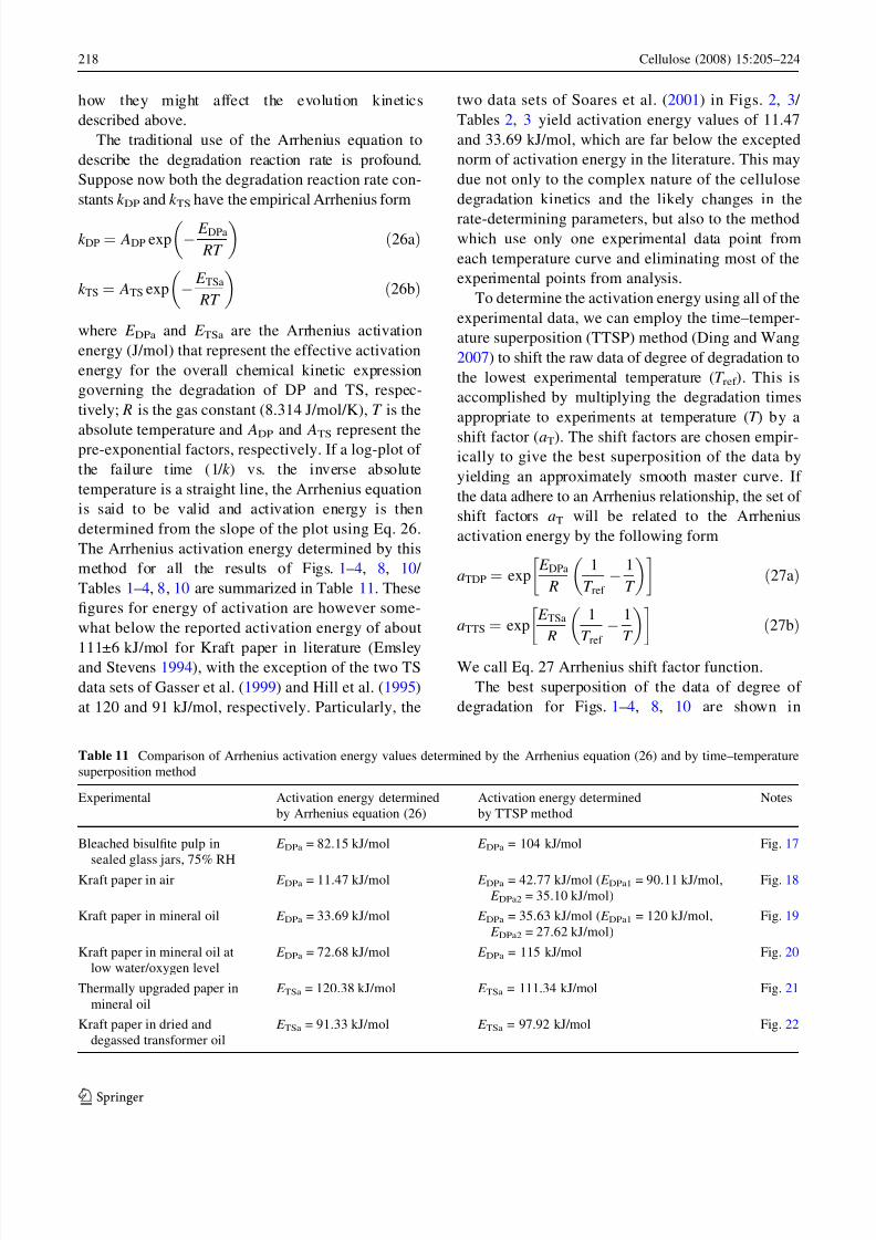
absolute temperature and ADP and ATS represent thepre-exponential factors, respectively. If a log-plot of the failure time (1/ k ) vs. the inverse absolutetemperature is a straight line, the Arrhenius equationis said to be valid and activation energy is thendetermined from the slope of the plot using Eq. 26.The Arrhenius activation energy determined by thismethod for all the results of Figs. 1–4, 8, 10 / Tables 1–4, 8, 10 are summarized in Table 11. Thesegures for energy of activation are however some-what below the reported activation energy of about

111±6 kJ/mol for Kraft paper in literature (Emsleyand Stevens 1994 ), with the exception of the two TSdata sets of Gasser et al. ( 1999 ) and Hill et al. ( 1995 )at 120 and 91 kJ/mol, respectively. Particularly, the

two data sets of Soares et al. ( 2001 ) in Figs. 2, 3 / Tables 2, 3 yield activation energy values of 11.47and 33.69 kJ/mol, which are far below the exceptednorm of activation energy in the literature. This maydue not only to the complex nature of the cellulosedegradation kinetics and the likely changes in the

rate-determining parameters, but also to the methodwhich use only one experimental data point fromeach temperature curve and eliminating most of theexperimental points from analysis.

To determine the activation energy using all of theexperimental data, we can employ the time–temper-ature superposition (TTSP) method (Ding and Wang2007 ) to shift the raw data of degree of degradation tothe lowest experimental temperature ( T ref ). This isaccomplished by multiplying the degradation timesappropriate to experiments at temperature ( T ) by a

shift factor ( a T ). The shift factors are chosen empir-ically to give the best superposition of the data byyielding an approximately smooth master curve. If the data adhere to an Arrhenius relationship, the set of shift factors aT will be related to the Arrheniusactivation energy by the following form

a TDP ¼ exp E DPa

R1

T ref

1T ð27a Þ

a TTS ¼ exp E TSa

R1

T ref

1T ð27b Þ

We call Eq. 27 Arrhenius shift factor function.The best superposition of the data of degree of

degradation for Figs. 1–4, 8, 10 are shown in

Table 11 Comparison of Arrhenius activation energy values determined by the Arrhenius equation (26) and by time–temperaturesuperposition method

Experimental Activation energy determinedby Arrhenius equation (26)

Activation energy determinedby TTSP method

Notes

Bleached bisulte pulp insealed glass jars, 75% RH

E DPa = 82.15 kJ/mol E DPa = 104 kJ/mol Fig. 17

Kraft paper in air E DPa = 11.47 kJ/mol E DPa = 42.77 kJ/mol ( E DPa1 = 90.11 kJ/mol,E DPa2 = 35.10 kJ/mol)

Fig. 18

Kraft paper in mineral oil E DPa = 33.69 kJ/mol E DPa = 35.63 kJ/mol ( E DPa1 = 120 kJ/mol,E DPa2 = 27.62 kJ/mol)

Fig. 19

Kraft paper in mineral oil atlow water/oxygen level

E DPa = 72.68 kJ/mol E DPa = 115 kJ/mol Fig. 20

Thermally upgraded paper inmineral oil

E TSa = 120.38 kJ/mol E TSa = 111.34 kJ/mol Fig. 21

Kraft paper in dried anddegassed transformer oil

E TSa = 91.33 kJ/mol E TSa = 97.92 kJ/mol Fig. 22

218 Cellulose (2008) 15:205–224

1 3

8/12/2019 On the Degradation Evolution Equations of Cellulose

http://slidepdf.com/reader/full/on-the-degradation-evolution-equations-of-cellulose 15/20

Figs. 11–16; and the corresponding Arrhenius plotsof the associated empirical shift factor values areshown in Figs. 17–22, respectively. Because of thelarge differences in experimental temperature condi-tions, the data for each condition are plottedseparately for the sake of visual clarity. The Arrhe-

nius activation energy determined by the TTSPmethod for all the results of Figs. 11–16 are alsosummarized in Table 11. Obviously, all these guresfor energy of activation are now in good agreementwith the reported activation energy of 111±6 kJ/molfor Kraft paper in literature (Emsley and Stevens1994 ), excepting for the two data sets of Soares et al.(2001 ) at 42.77 and 35.63 kJ/mol, respectively,which are still well below the excepted norm of activation energy in the literature.

Further studies in Figs. 18 and 19 have foundthat for the experimental data obtained in air, attemperatures of 90 C and below the activationenergy value is equal to approximately 90 kJ/mol,and the data above 90 C seems to imply acurvature to a smaller activation energy value of 35.10 kJ/mol; and for the experimental dataobtained in mineral oil, at temperatures of 80 Cand below the activation energy value is equal toapproximately 120 kJ/mol, and the data above80 C seems to imply a curvature to a smalleractivation energy value of 27.62 kJ/mol. The‘‘downward’’ curvature in the Arrhenius plotsobserved for both the experimental data obtainedin air (Fig. 18) and the experimental data obtainedin mineral oil (Fig. 19) indicates that a change inthe mix of DP degradation reactions is occurringwith degradation temperature for the Kraft paperstudied. Generally speaking, such curvature impliesthat certain higher activation energy processes arebecoming less important at higher degradationtemperatures. This is the evidence of non-Arrheniusbehaviour, and similar phenomena have beenreported in the literature for some polymers (Gillenet al. 2005a , b).

Towards a new method for the prediction of cellulose degradation at ambient conditions

All master curves in Figs. 11–14 can be further ttedby Eq. 18 to yield corresponding master equation

representing the kinetics of percentage DP loss asfollows.

(1) For the DP data of BBSP handsheets aged inseal vessels and 75% RH in Fig. 11:

1 DP

DP 0¼ 0 : 780 1 e 0: 0043 a TDP t T

ð28a Þ

a TDP ¼ exp 12 ; 509 1

273 þ 60 1

273 þ T ð28b Þ

where t T is the degradation time by days at thetemperature T in Celsius.(2) For the DP data of Kraft paper aged in air

Fig. 12:

1 DP

DP 0

¼ 0 : 480 1 e 0: 0032 a TDP t T

ð29a Þ

a TDP ¼ exp 10 ; 838 1

273 þ 70 1

273 þ T ð29b Þ

where t T is the degradation time by hours at thetemperature T in Celsius.(3) For the DP data of Kraft paper aged in mineral

oil at high water/oxygen level in Fig. 13:

1 DPDP 0

¼ 0 : 750 1 e 0: 0002 a TDP t T

ð30a Þ

0 100 200 300 400 500 600 700 8000.0

0.2

0.4

0.6

0.8

1.0

TTSP master curve R 2 = 0.9872

, n o i t a

d a r g e

d f o e e r g e

D

ω P D

Shift time (=a T* ageing time) at 60 oC, days

Temperature a T

60 oC 170 oC 3.3

80 oC 8.4 90 oC 26 100 oC 54

Fig. 11 Time–temperature superposition of the degree of degradation data from Fig. 1 at 60 C using the shift factorsas shown in the gure

Cellulose (2008) 15:205–224 219

1 3

8/12/2019 On the Degradation Evolution Equations of Cellulose

http://slidepdf.com/reader/full/on-the-degradation-evolution-equations-of-cellulose 16/20

a TDP ¼ exp 14433 : 49 1

273 þ 65 1

273 þ T ð30b Þ

where t T is the degradation time by hours at thetemperature T in Celsius.(4) For the DP data of Kraft paper aged in mineral

oil at low water/oxygen level in Fig. 14:

1 DPDP 0

¼ 0 : 900 1 e 0: 0003 a TDP t T ð31a Þ

a TDP ¼ exp 13 ; 832 1273 þ 120

1273 þ T

ð31b Þ

where t T is the degradation time by hours at thetemperature T in Celsius.

Similarly, master curves in Figs. 15, 16 can befurther tted by Eq. 23 to produce correspondingmaster equation representing the kinetics of percent-age TS loss as follows.

(5) For the TS data of thermally upgraded insula-tion paper aged in closed system with mineraloil in Fig. 15:

0 500 1000 1500 20000.0

0.2

0.4

0.6

0.8

1.0

TTSP master curve R 2=0.9524

Temperature aT

70 oC 1 80 oC 2.4 90 oC 5.6 105 oC 8 120 oC 13

D e

, n o i t a

d a r g e d f o e e r g

ω P D

Shift time (= a T* ageing time) at 70 oC, hours

Fig. 12 Time–temperature superposition of the degree of degradation data from Fig. 2 at 70 C using the shift factorsas shown in the gure

0 20000 40000 600000.0

0.2

0.4

0.6

0.8

1.0

TTSP master curve R 2 = 0.9648

, n o i t a

d a r g e

d f o e e r g e

D

ω P D

Shift time (=aT* ageing time) at 65 oC, hours

Tempe ra tu re a T

65 oC 1 80 oC 6.4 120 oC 16

Fig. 13 Time–temperature superposition of the degree of degradation data from Fig. 3 at 65 C using the shift factorsas shown in the gure

0 20000 40000 60000 80000 1000000.0

0.2

0.4

0.6

0.8

1.0

TTSP master curve R 2=0.9616 ,

n o i t a

d a r g e

d f o e e r g e

D

ω P D

Shift time (=aT* ageing time) at 120 oC, hours

Tem pe ra tu re a T

120 oC 1140 oC 5.50

160 oC 2 5.8 3

Fig. 14 Time–temperature superposition of the degree of degradation data from Fig. 4 at 120 C using the shift factorsas shown in the gure

0 200 400 600 800 1000 12000.0

0.2

0.4

0.6

0.8

1.0

TTSP master curveR2=0.9874

, n o i t a

d a r g e

d f o e e r g e

D

ω S T

Shift time (=a T* ageing time) at 120 oC, days

Temperature a T

120 oC 1 130 oC 2.3 150 oC 11.1

Fig. 15 Time–temperature superposition of the degree of degradation data from Fig. 8 at 120 C using the shift factorsas shown in the gure

220 Cellulose (2008) 15:205–224

1 3

8/12/2019 On the Degradation Evolution Equations of Cellulose

http://slidepdf.com/reader/full/on-the-degradation-evolution-equations-of-cellulose 17/20

1 TSTS 0

¼ 0 : 594 1 e 0 : 0028 a TTS t T ð32a Þ

a TTS ¼ exp 13391 : 87 1

273 þ 120 1

273 þ T ð32b Þ

where t T is the degradation time by days at thetemperature T in Celsius.(6) For the TS data of Kraft insulation paper aged in

dried and degassed transformer oil in Fig. 16:

1 TSTS 0

¼ 0 : 810 1 e 0 : 0153 a TTS t T ð33a Þ

a TTS ¼ exp 11777 : 72 1

273 þ 129 1

273 þ T ð33b Þ

where t T is the degradation time by days at thetemperature T in Celsius.

According to master equations (28)–(33), itbecomes possible to quantitatively predict the degreeof degradation of cellulose at ambient operatingconditions. Let us look at two examples. According toEq. 28, the extrapolated shift factor aTDP will bea TDP = 0.0091 at 23 C, which implies that withsame relative humidity of 75%, the time required toreach a given level of degree of degradation at 23 C

will be 110 times that required at the referencetemperature of 60 C; and the degree of degradationof BBSP paper in terms of the percentage DP loss

0 50 100 150 200 250 3000.0

0.2

0.4

0.6

0.8

1.0

TTSP master curve

R2=0.9703 ,

n o i t a

d a r g e

d f o e e r g e

D

ω S T

Shift time (=a T* ageing time), days

Temperature a T

129 oC 1 138 oC 1.9 153 oC 5.2 166 oC 11.8

Fig. 16 Time–temperature superposition of the degree of degradation data from Fig. 10 at 129 C using the shift factorsas shown in the gure

2.6 2.8 3.0 3.210 -1

10 0

10 1

10 2

E D P a = 8 2.

1 5 k J /

m o l, R 2 = 0. 9 9

4 0

Empirical shift factor a T

/ 1 ( n l

k P D

)

E D P a = 1 0 4 k J / m o l , R 2

= 0 .9 9 0 7

p m

E

i

h s l

a c i r

i

a , r o t c a f t f

T

1000/T, K -1

1

2

3

4

5

6

7 DP degradation rate k

DP

Fig. 17 Arrhenius plots for the DP degradation rate k DP datain Table 1 and for the empirical values of the shift factors aT

used to superpose degree of degradation data from Fig. 11

2.40 2.55 2.70 2.85 3.0010 -1

10 0

10 1

10 2

E D P a 2 = .5 3 1 k J / m o l , R 2

= .0 9 5 0 9

Empirical shift factor a T

E D P a = 11. 4 7 k / J m o l, R

2 = 0. 91 4 9

/ 1 ( n l

k P D

)E D P a = 4 2 .7 7 k J / m o l , R 2

= 0 .9 7 1 9

E D P a 1 = 9 0 .1 1 k J / m o l , R 2

= 1

i h s l a c i r i p m

E

a , r o t c a f t f

T

1000/T, K -1

3

4

5

6 DP degradation rate k

DP

Fig. 18 Arrhenius plots for the DP degradation rate k DP datain Table 2 and for the empirical values of the shift factors aT

used to superpose degree of degradation data from Fig. 12

2.40 2.55 2.70 2.85 3.0010 -1

10 0

10 1

10 2Empirical shift factor a

T

E D P a = 3 3. 6 9 k J / m o l, R

2 = 0. 9 0 5 2

E D P a = 3 5 .6 3 k J / m o l , R 2

= 0 .9 5 5 8

E D a P 2 = 2 7 .6 2 k J / m o l , R 2

= 1

E P D a 1 =

2 1 0 k J m /

, l o R 2

1 =

m E

r i p

i l a c

a f t f i h s

a , r o t c

T

1000/T, K -1

6

8

10

12

14DP degradation rate k

DP

/ 1 ( n l

k P D

)

Fig. 19 Arrhenius plots for the DP degradation rate k DP datain Table 3 and for the empirical values of the shift factors aT

used to superpose degree of degradation data from Fig. 13

Cellulose (2008) 15:205–224 221

1 3

8/12/2019 On the Degradation Evolution Equations of Cellulose

http://slidepdf.com/reader/full/on-the-degradation-evolution-equations-of-cellulose 18/20

will reach 39.8% after 10 years, 59.3% after100 years and 77.9% after 500 years. According toEq. 32, the extrapolated shift factor aTTS will bea TTS = 0.0070 at 70 C (normal transformer opera-tion temperature), which implies that with sameexperimental conditions, the degree of degradation of

thermally upgraded insulation paper in terms of percentage TS loss will reach 4.1% after 10 years,17.86% after 50 years and 30.35% after 100 years.Admittedly, these are approximate values. However,the results described above illustrate a new methodfor prediction of cellulose degradation at ambientconditions.

Conclusions

The present study investigates the degradation evo-lution equation of cellulose. From the results obtainedin the present study the following conclusions aredrawn.

(1) Cellulose degradation can be best characterizedin terms of the percentage DP loss. Thedegradation variable x DP can be calculatedthrough the measured degree of polymerisationof a cellulose, DP 0 , and the effective degree of polymerisation after degradation occurred, DP,

in terms of the denition x DP:

1–DP/DP 0 .Different values of the degradation variablecorrespond to different states of the cellulose as(a) x DP = 0 corresponds to the undegradedstate; (b) x DP = 1 corresponds to the fully-degraded state (i.e., failure); and (c) 0 \ x DP \

1 corresponds to the degraded state.(2) A new cellulose degradation evolution equation

expressed in terms of the percentage DP loss hasbeen presented and applied to have a quantita-tive comparison with six sets of experimental

results. The results show that the new cellulosedegradation evolution equation ( 18) is able toexplain the real experimental data of differentcellulose materials under a variety of experi-mental conditions, particularly the prolongedautocatalytic degradation in sealed vessels.

(3) Cellulose degradation can be best characterizedalso in terms of the percentage TS loss. Thedegradation variable x TS can be calculatedthrough the measured tensile strength of a

2.2 2.3 2.4 2.5 2.6

10 0

10 1

10 2

/ 1 (

n l

k P D

)

, r o t c a f t f i

h s l

a c i r i p m

E

a T

E D P a = 7 2.

6 8 k J /

m o l, R 2 = 0. 9 8 8 6

Empirical shift factor a T

E D P a = 1 1 5 k J / m o l , R 2 = 1

1000/T, K -1

4

5

6

7

8 DP degradation rate k

DP

Fig. 20 Arrhenius plots for the DP degradation rate k DP datain Table 4 and for the empirical values of the shift factors aT

used to superpose degree of degradation data from Fig. 14

2.3 2.4 2.5 2.6

10 0

10 1

10 2

/ 1 ( n l

k S T

)

E T S a = 1 2 0

. 3 8 k J /

m o l, R

2 = 0. 9 6 0 6

Empirical shift factora

T

E T S a = 1 1 1 3 . 4 k J m / o l , R 2

= 1

p m

E

i

h s l a c i r

i

a , r o t c a f t f

T

1000/T, K -1

3

4

5

6

7TS degradation rate k

TS

Fig. 21 Arrhenius plots for the TS degradation rate k TS data inTable 8 and for the empirical values of the shift factors aT usedto superpose degree of degradation data from Fig. 15

2.2 2.3 2.4 2.5 2.610 -1

10 0

10 1

10 2

E T S a = 9 1

3. 3 k J m / o l R,

2 = 0 9. 6 0 4

Empirical shift factor a T

/ 1 ( n l

k S T

)

E T S a = 9 7 .9 2 k J / m o l , R 2

= 1

p m

E

i

h s l a

c i r

i

a , r o t c a f t f

T

1000/T, K -1

1

2

3

4

5

6TS degradation rate k

TS

Fig. 22 Arrhenius plots for the TS degradation rate k TS data inTable 10 and for the empirical values of the shift factors aT

used to superpose degree of degradation data from Fig. 16

222 Cellulose (2008) 15:205–224

1 3

8/12/2019 On the Degradation Evolution Equations of Cellulose

http://slidepdf.com/reader/full/on-the-degradation-evolution-equations-of-cellulose 19/20

cellulose, TS 0 , and the effective tensile strengthafter degradation occurred, TS, in terms of thedenition x TS : 1–TS/TS 0 . A new kineticequation ( 23) for loss of tensile strength of cellulose, which is analogous to the new cellu-lose degradation evolution equation ( 18), has

been presented and applied to explain four setsof experimental data of tensile strength. Theresults show that the good agreement betweenthe predictions and experimental data appears tobe justied in principle.

(4) A new method for prediction of cellulosedegradation at ambient conditions has beendeveloped by combining the master equationrepresenting the kinetics of either percentageDP loss or percentage TS loss at the lowestexperimental temperature with Arrhenius shift

factor function.(5) It is critical to model the cellulose degradation

evolution kinetics accurately for degradationprediction. The proposed degradation evolutionequations expressed in terms of either thepercentage DP loss or the percentage TS lossappear to accomplish this with good accuracyfor the experimental data considered. However,additional theoretical and experimental studiesare suggested to conrm the proposed cellulosedegradation evolution equations ( 18) and (23).

Acknowledgements We would like to thank all anonymousreviewers for some very valuable suggestions. We would alsolike to thank Professor Wolfgang Glasser (Editor in Chief) forencouragement. The research was partly supported by theEPSRC-SUPERGEN V-AMPerES (Asset Management andPerformance of Energy Systems).

References

Arney JS, Noval CL (1982) Accelerated aging of paper. Theinuence of acidity on the relative contribution of oxygen-independent and oxygen-dependent processes. Tappi J65:113–115

Baran ski A, Łagan JM, Łojewski T (2006) The concept of mixed-control mechanisms and its applicability to paperdegradation studies. e-PS 3:1–4

Bouchard J, Me´thot M, Jordan B (2006) The effects of ionizingradiation on the cellulose of woodfree paper. Cellulose13:601–610

Calvini P (2005) The inuence of levelling-off degree of polymerisation on the kinetics of cellulose degradation.Cellulose 12:445–447

Calvini P, Gorassini A (2006) On the rate of paper degradation:lessons from the past. Restaurator 27(4):275–290

Chen SL, Lucia LA (2003) Improved method for evaluation of cellulose degradation. J Wood Sci 49:285–288

Daruwalla EH, Narsian MG (1966) Detection and identicationof acid-sensitive linkages in cellulose ber substances.Tappi J 49(3):106–111

Ding H-Z, Wang ZD (2007) Time–temperature superpositionmethod for predicting the permanence of paper byextrapolating accelerated ageing data to ambient condi-tions. Cellulose 14:171–181

Ekenstam A (1936) The behaviour of cellulose in mineral acidsolutions: kinetic study of the decomposition of cellulosein acid solutions. BER 69:540–553

Emsley AM, Stevens GC (1994) Kinetics and mechanisms of the low temperature degradation of cellulose. Cellulose1:26–56

Emsley AM, Heywood RJ, Ali M, Eley CM (1997) On thekinetics of degradation of cellulose. Cellulose 4:1–5

Emsley AM, Xiao X, Heywood RJ, Ali M (2000a) Degradationof cellulosic insulation in power transformers. Part 3:

effects of oxygen and water on ageing in oil. IEE Proc SciMeas Technol 147(3):115–119

Emsley AM, Heywood RJ, Ali M, Xiao X (2000b) Degradationof cellulosic insulation in power transformers. Part 4:effects of ageing on the tensile strength of paper. IEE ProcSci Meas Technol 147(6):285–290

Feller RL, Lee SB, Bogaard J (1986) The kinetics of cellulosedeterioration. In: Needles HL, Zeronian SH (eds) Historictextile and paper materials: conservation and character-ization. Advances in chemistry series 212. AmericanChemical Society, Philadelphia, USA, pp 329–346

Fung DPC (1969) Kinetics and mechanism of the thermaldegradation of cellulose. Tappi J 52:319–321

Gasser HP, Huser J, Krause C, Dahinden V, Emsley AM(1999) Determining the ageing parameters of cellulosicinsulation in a transformer. In: Eleventh internationalsymposium on high voltage engineering (IEE Conf. Publ.No. 467), London, 23–27 August 1999, pp 4.143–4.147

Gillen KT, Bernstein R, Derzon DK (2005a) Evidence of non-Arrhenius behaviour from laboratory aging and 24-yearseld aging of polychloroprene rubber materials. Poly DegStab 87:57–67

Gillen KT, Bernstein R, Celina M (2005b) Non-Arrheniusbehavior for oxidative degradation of chlorosulfonatedpolyethylene materials. Poly Deg Stab 87:335–346

Hansen AC, Baker-Jarvis J (1990) A rate-dependent kinetictheory of fracture for polymers. Inter J Fracture 44:221–231

Heywood RJ, Stevens GC, Ferguson C, Emsley AM (1999)Life assessment of cable paper using slow thermal rampmethod. Thermochim Acta 332:189–195

Hill DJT, Le TT, Darveniza M, Saha T (1995) A study of degradation of cellulosic insulation materials in a powertransformer. Part 2: tensile strength of cellulose insulationpaper. Polym Deg Stab 49:429–435

Hon DNS (1985) Mechanochemistry of cellulosic materials. In:Kennedy JF, Phillips GO, Wedlock DJ, Williams PA (eds)Cellulose and its derivatives: chemistry, biochemistry andapplications, chapter 6. Ellis Horwood Limited, Chiches-ter, UK, pp 71–86

Cellulose (2008) 15:205–224 223

1 3

8/12/2019 On the Degradation Evolution Equations of Cellulose

http://slidepdf.com/reader/full/on-the-degradation-evolution-equations-of-cellulose 20/20

Johansson EE, Lind J, Ljunggren S (2000) Aspects of thechemistry of cellulose degradation and the effect of eth-ylene glycol during ozone delignication of Kraft pulps. JPulp Pap Sci 26:239–244

Krassig H, Kitchen W (1961) Factors inuencing tensileproperties of cellulose bers. J Polym Sci 51:123–172

Kukensko VS, Tamuzs VP (1981) Fracture micromechanics of polymer materials.Martinus Nijhoff Publishers,Boston, MA

Margutti S, Conio G, Calvini P, Pedemonte E (2001) Hydrolyticand oxidative degradation of paper. Restaurator 22:67–83

McCrady E (1996) Effect of metals on paper: a literaturereview. Alkaline Paper Advocate, vol 9(1), May

McShane CP, Corkran JL, Rapp KJ, Luksich J (2003) Aging of paper insulation retrolled with natural ester dielectricuid. IEEE 2003 annualreport conf. on electrical insulationand dielectric phenomena. Albuquerque, USA,pp 124–127

Moser HP, Dahinden V (1987) Transformerboard II. H. We-idmann AG, CH-8640 Rapperswil

Petrov VA (1984) Lifetime-under-load of solid subjected tostresses below the breaking value. Sov Phys Solid State26:1283–1284

Shazadeh F, Bradbury AGW (1979) Thermal degradation of cellulose in air and nitrogen at low temperatures. J ApplPolym Sci 23:1431–1442

Sharples A (1954) The hydrolysis of cellulose. Part 1. The nestructure of Egyptian cotton. J Polym Sci 13:393–401

Sharples A (1971) Degradation of cellulose and its derivatives.A. Acid hydrolysis and alcoholysis. In: Bikales NM, Segal

L (eds) Cellulose and cellulose derivatives, vol V, Pt V.Wiley-Interscience, New York, pp 991–1006

Soares S, Ricardo N, Heatley F, Rodrigues E (2001) Lowtemperature thermal degradation of cellulosic insulatingpaper in air and transformer oil. Polym Int 50:303–308

Strlic M, Kolar J, Pihlar B, Rychly ´ J, Matisova -Rychla L(2001) Initial degradation process of cellulose at elevatedtemperatures revisited-chemiluminescence evidence.Polym Deg Stab 72:157–162

Testa G, Sardella A, Rossi E, Bozzi C, Seves A (1994) Thekinetics of cellulose ber degradation and correlation withsome tensile properties. Acta Polymer 45:47–49

Williams JC, Fowler CS, Lyon MS, Merrill TL (1977) Metalliccatalysts in the oxidative degradation of paper. Advancesin chemistry series, ACS 164, pp 37–61

Zervos S, Moropoulou A (2005) Cotton cellulose ageing insealed vessels. Kinetic model of autocatalytic depoly-merization. Cellulose 12:485–496

Zhurkov SN, Korsukov VE (1974) Atomic mechanism of fracture of solid polymers. J Polym Sci: Polym Phys12:385–398

Zou X, Gurnagul N, Uesaka T, Bouchard J (1994) Acceleratedageing of papers of pure cellulose: mechanism of cellu-lose degradation and paper embrittlement. Polym DegStab 43:393–402

Zou X, Uesaka T, Gurnagul N (1996) Prediction of paperpermanence by accelerated ageing: Part 1 kinetic analysisof the aging process. Cellulose 3:243–267

224 Cellulose (2008) 15:205–224

1 3