on the design and testing of ocean wave energy convertor.pdf
TRANSCRIPT

AN ABSTRACT OF THE DISSERTATION OF
Bret Bosma for the degree of Doctor of Philosophy in Electrical and Computer
Engineering presented on July 16, 2013.
Title: On the Design, Modeling, and Testing of Ocean Wave Energy Converters.
Abstract approved: ______________________________________________________
Ted K.A. Brekken
Ocean wave energy converter technology continues to advance and new developers
continue to emerge, leading to the need for a general design, modeling, and testing
methodology. This work presents a development of the process of taking a wave energy
converter from a concept to the prototype stage. A two body heaving point absorber
representing a generic popular design was chosen and a general procedure is presented
showing the process to model a wave energy converter in the frequency and time
domains. A scaled prototype of an autonomous small scale wave energy converter was
designed, built, and tested and provided data for model validation. The result is a guide
that new developers can adapt to their particular design and wave conditions, which will
provide a path toward a cost of energy estimate. This will serve the industry by
providing sound methodology to accelerate the continued development of wave energy
converters.

©Copyright by Bret Bosma
July 16, 2013
All Rights Reserved

On the Design, Modeling, and Testing of Ocean Wave Energy Converters
by
Bret Bosma
A DISSERTATION
submitted to
Oregon State University
in partial fulfillment of
the requirements for the
degree of
Doctor of Philosophy
Presented July 16, 2013
Commencement June 2014

Doctor of Philosophy dissertation of Bret Bosma presented on July 16, 2013
APPROVED:
_____________________________________________________________________
Major Professor, representing Electrical and Computer Engineering
_____________________________________________________________________
Director of the School of Electrical Engineering and Computer Science
_____________________________________________________________________
Dean of the Graduate School
I understand that my dissertation will become part of the permanent collection of
Oregon State University libraries. My signature below authorizes release of my
dissertation to any reader upon request.
_____________________________________________________________________
Bret Bosma, Author

ACKNOWLEDGEMENTS
I would like to give special thanks to my advisor Dr. Ted Brekken for his guidance,
support, and enthusiasm toward renewable energy research. Also, thanks goes to my
committee members Dr. Annette von Jouanne, Dr. Ean Amon, Dr. Solomon Yim, and
Dr. Joe Zaworski who all contributed significantly to my time here at Oregon State.
Thanks also goes to the whole Energy Systems Research group for being such a
fun, strong, and focused team to work with. I would like to give special thanks to Doug
Halamay and Chris Haller for their camaraderie in the lab. Thanks to Tim Lewis for a
great collaboration on the AWEC project. Thanks to Stephen Zhang for all of the
modeling help and wave energy discussions. Thanks to Kelley Ruehl for a great
collaboration early on. In addition, I would like to thank the Northwest National Marine
Renewable Energy Center, and specifically Belinda Batten and Meleah Ashford for their
support during my time here. Thanks also to Manfred Dittrich for being patient with
me and building an awesome prototype.
Finally, and most importantly, I want to thank my fiancé Emily, my Mom, and my
Dad. Without your love and encouragement this would not have been possible. Thank
you.

TABLE OF CONTENTS
Page
1 Introduction .............................................................................................................. 1
2 Frequency Domain Analysis .................................................................................... 7
2.1 Introduction ......................................................................................................7
2.1.1 Linear Wave Theory ..............................................................................9
2.1.2 Forces on Structures ............................................................................10
2.1.3 RAOs ............................................................................................. 12
2.1.4 Workflow .............................................................................................14
2.2 Device Geometry ...........................................................................................15
2.2.1 Solid Model .........................................................................................17
2.2.2 Mass Properties ...................................................................................18
2.3 Wave Resource Data ......................................................................................19
2.3.1 Range and Number of Frequencies .....................................................20
2.3.2 Wave Directions ..................................................................................20
2.3.3 Water Depth ........................................................................................20
2.4 Hydrodynamic Software Packages ................................................................21
2.4.1 3-D Diffraction and Radiation Analysis ..............................................22

TABLE OF CONTENTS (Continued)
Page
2.4.2 Equilibrium and Stability Analysis .....................................................24
2.4.3 Frequency Domain Analysis ...............................................................24
2.4.4 Mooring Model (Linearized) ...............................................................24
2.4.5 Power Take Off Model (Linearized) ...................................................25
2.4.6 Response Amplitude Operators (RAOs) .............................................25
2.5 Output Power Comparisons ...........................................................................26
2.6 Conclusions ....................................................................................................27
3 Time Domain Analysis .......................................................................................... 29
3.1 Introduction ....................................................................................................29
3.1.1 Background .........................................................................................29
3.1.2 Equations of Motion ............................................................................31
3.2 Model to be Analyzed ....................................................................................33
3.3 Input Waves ...................................................................................................35
3.3.1 Regular Waves ....................................................................................35
3.3.2 Irregular Waves ...................................................................................36
3.4 Time Domain Differential Equation Solver Approach ..................................36
3.5 Simulation Results .........................................................................................40
TABLE OF CONTENTS (Continued)
Page
3.6 Conclusions ....................................................................................................43
4 Wave Tank Testing and Model Validation ............................................................ 44
4.1 Introduction ....................................................................................................44
4.2 Device Geometry, Scaling, Power Take Off, and Mooring ...........................45
4.2.1 Geometry .............................................................................................46
4.2.2 Scaling ............................................................................................. 47
4.2.3 Power Take Off ...................................................................................49
4.2.4 Mooring ............................................................................................. 50
4.3 Linear Test Bed Testing .................................................................................50
4.3.1 Power Delivered to the Load ...............................................................52
4.3.2 Efficiency Test ....................................................................................52
4.3.3 Estimated Damping Values Due to Losses .........................................54
4.4 Wave Tank Testing Facilities ........................................................................55
4.4.1 Large Wave Flume ..............................................................................55
4.4.2 Optical Motion Capture System ..........................................................57
4.4.3 Mooring ............................................................................................. 58

TABLE OF CONTENTS (Continued)
Page
4.4.4 Device Performance Data ....................................................................58
4.5 Wave Tank Testing Procedure .......................................................................60
4.5.1 Experimental Methodology and Procedure .........................................60
4.5.2 Types of Trials Conducted ..................................................................61
4.6 Wave Tank Testing Results ...........................................................................61
4.6.1 Commanded vs. Measured Wave Tank Results ..................................62
4.6.2 Max Damping Value ...........................................................................63
4.6.3 Response Amplitude Operators (RAOs) .............................................64
4.6.4 Power Characteristics ..........................................................................66
4.7 Conclusions ....................................................................................................68
5 Conclusion ............................................................................................................. 70
5.1 Recommendation for Future Work ................................................................71
6 Bibliography ........................................................................................................... 72

LIST OF FIGURES
Figure Page
Fig. 1.1. WEC Design Flow Chart ................................................................................ 5
Fig. 2.1. High Level block diagram of inputs and outputs of frequency domain model.
........................................................................................................................................ 9
Fig. 2.2. Equation of motion terms of fluid forces on a structure. .............................. 14
Fig. 2.3. Example workflow for frequency domain analysis. ..................................... 15
Fig. 2.4. Generic WEC example. A massless, stiff connection between the spar and
damper is present, but not shown. All dimensions in meters. ..................................... 16
Fig. 2.5. Example 3-D Diffraction and Radiation Analysis results. ........................... 23
Fig. 2.6. RAO amplitude and phase for each body. .................................................... 26
Fig. 2.7. Power vs. Frequency plot for multiple damping values, including envelope
(thick black line) showing max power output for each frequency which could be
achieved using active damping. ................................................................................... 27
Fig. 3.1. Time domain formulation and analysis block diagram. ............................... 30
Fig. 3.2. Generic WEC example. All Dimensions in meters. .................................... 34
Fig. 3.3. MATLAB/Simulink implementation of equations of motion for two body
WEC. ............................................................................................................................ 37
Fig. 3.4. Excitation Force convolution. ....................................................................... 39
Fig. 3.5. Linear damping regular wave input. ............................................................. 41
Fig. 3.6. Linear damping regular wave input. The PTO force is clipped at 200kN to
represent realistic limitations of physical equipment. Because of this nonlinearity this
analysis must be done in the time domain. .................................................................. 41
Fig. 3.7. Linear damping irregular wave input............................................................ 42
Fig. 3.8. Linear damping irregular wave input. The PTO force is clipped at 100kN to
represent realistic limitations of physical equipment. Because of this nonlinearity this
analysis must be done in the time domain. .................................................................. 42
Fig. 4.1. Scaled wave tank testing block diagram. Scaled model wave tank testing for
use in model validation. ............................................................................................... 45
LIST OF FIGURES (Continued)
Figure Page
Fig. 4.2. Autonomous Wave Energy Converter: (a) Full Scale and (b) ¼ scale. All
dimensions in meters. ................................................................................................... 47
Table 1: Froude Scaling for the AWEC ...................................................................... 48
Fig. 4.3. Testing in the Linear Test Bed (LTB) ........................................................... 51
Fig. 4.4. Power Delivered to the Load in Watts. Power generally increases as velocity
increases. A load resistance near the generator internal resistance (7.41 ohms) provides
max power. ................................................................................................................... 52
Fig. 4.5. Total PTO efficiency in % for different velocities and loads. As speed
increases, so does efficiency. The efficiency peaks for the generator load at
approximately twice the generator internal resistance (7.41 ohms). ............................ 53
Fig. 4.6. Estimated Loss Damping Values for a Sweep of Velocity and Load Values.
Higher speeds produced lower estimated damping values. ......................................... 55
Fig. 4.7. Large Wave Flume Configuration ................................................................ 57
Fig. 4.8. Optical Motion Tracking: (a) Setup in HWRL and (b) screen capture of
tracking markers. .......................................................................................................... 58
Fig. 4.9. Power Take Off circuit. ................................................................................ 59
Fig. 4.10. AWEC testing in the Hinsdale Wave Research Laboratory at Oregon State
University. .................................................................................................................... 60
Fig. 4.11. Average Power vs. Damping for two monochromatic wave inputs. .......... 64
Fig. 4.12. RAOs for HWRL, AQWA, and MATLAB. ............................................... 66
Fig. 4.13. Power Matrix for Irregular wave input: (a) HWRL wave tank testing, (b)
AQWA model, and (c) MATLAB model. ................................................................... 67
Fig. 4.14. Percent error between measured tank testing data and AQWA model data.
AQWA over-predicts for lower significant wave heights and dominant periods.
AQWA under-predicts for higher significant wave heights and dominant periods. .... 68

On The Design, Modeling, and Testing of Wave Energy Converters
1 Introduction
The worlds growing energy demand coupled with climate change concerns have
led to a resurgence of interest in renewable energy technologies [1]. It has become clear
that we will need a host of solutions both renewable and non-renewable in order to keep
up with world electricity demand. Solar and wind technologies have gradually matured
with wind power becoming cost competitive in many energy markets. Ocean wave
energy presents a vast, largely untapped, energy resource with the potential to add to
the renewable energy mix.
Harnessing energy from ocean waves is not a new concept. The first patent of
techniques for extracting energy from ocean waves dates back to 1799 [2]. The
development of devices since has seen ups and downs including a resurgence in the
1970’s with the research of Stephen Salter and the development of Salter’s Duck [3].
Since then, there has been varying activity in the field with popularity and significant
research increasing recently. Of note, Michael McCormick and Johannes Falnes have
done pioneering research in the field.
The ocean provides the potential for an enormous untapped resource. In 2011 the
Electric Power Research Institute (EPRI) did a study mapping and assessing the United
States ocean wave energy resource [4]. They found that in total, electricity generation
from waves could amount to more than 1170 TWh/year. That is near one third of the
total annual consumption in the United States.
2
Ocean wave energy has many advantages. It is a renewable resource, generated
ultimately from the sun. The sun causes uneven heating of the earth’s surface which
creates wind. Wind blown over the ocean surface creates waves. It is relatively
predictable and consistent when compared to wind or solar. Although the resource can
vary quite a bit seasonally, day to day the resource is relatively constant. It is also
predictable in that sensors can be put out to sea and the resource at a location can be
predicted as much as 48 hours in advance. Wave energy devices also typically have a
low view shed. That is to say that typically most or all of the device is located under
the water surface.
Ocean wave energy extraction can also pose many challenges. The ocean is a harsh
environment and survivability is a key concern with extreme sea states and a caustic
environment. There are also potential environmental effects including harm to wildlife
and impact on sediment transport. Probably the biggest challenge to wave energy,
however, is the high cost associated with the technology. The device cost itself is high
and the deployment of the device is expensive. Operation and maintenance costs are
high. Transporting the energy from the generation site to where it can be used is costly.
For the wave energy industry to be successful these challenges will need to be
addressed.
There are many ideas of how to extract the energy from the ocean waves with new
concepts still being developed. Unlike the wind industry, where a horizontal two or
three blade turbine has become the clear choice, there is a wide variety of wave energy
technologies. These arise from the various ways that the energy can be absorbed from

3
the waves. Wave Energy Converters (WECs) can be classified in many ways including
size, proximity to shore, and working principal [5].
In general there are three dominant types of devices, namely the oscillating water
column, oscillating bodies, and overtopping type devices. Oscillating water columns
can be split into near-shore fixed structures such as the Limpet, and off-shore floating
structures such as the Oceanlinx. Oscillating bodies can be broken into floating types
such as the PowerBuoy and submerged types such as the Oyster. Overtopping devices
can be split into fixed structure types such as the TAPCHAN and floating structures
such as the Wave Dragon.
One of the promising technologies which has attracted many developers is the
heaving point absorber. A point absorber is defined as a device that has a horizontal
extent much smaller than the incoming wave length. A relatively simple device, a
heaving point absorber is an oscillating body which extracts the heave, or vertical
motion from a wave. Point absorbers can be single-body or multi-body devices with
hybrid type devices also possible.
Although the focus of this document is on the design, modeling, and testing of a
heaving point absorber, many of the principals can be applied to other types of devices.
For example, most systems will need hydrodynamic modeling as part of the design
process. The concepts behind the frequency domain, time domain, and scaled wave
tank testing will generally apply to other types of wave energy converters. Fig. 1.1
shows a block diagram of each major step in the process outlined in this document. The
4
tools used or developed are at the core of the diagrams and the necessary inputs and
outputs are also shown.
The Oregon Wave Energy Trust has published an adaptation of the U.S.
Department of Energy Guide that details Technology Readiness Levels (TRLs) for
ocean wave energy devices [6]. These TRLs are from 1-9 and describe each phase in
the process of commercialization of a wave energy converter. TRL 1 is basic
technology research in which basic principles are observed and reported and TRL 9 is
system operations at which the actual system is operated over its full range of expected
conditions. Aspects of TRLs 1-5 are detailed in this document.
Chapter 2 describes frequency domain analysis and is the first step in the
hydrodynamic modeling process. For this step everything is assumed to be linear, which
has the benefit of speed and ease of implementation. Assuming linearity allows for
rapid simulation times and is especially useful in shape optimization routines.
Furthermore, frequency domain analysis can be the basis for a time domain analysis
where nonlinearities can be introduced. This work falls into TRLs 1-2.
Chapter 3 outlines the time domain analysis which takes the frequency domain
results and transfers them to the time domain. Among the advantages to this approach
are the application of any input waveform that is desired and the introduction of
nonlinearities to the system. This provides a higher level of detail of the operation of
the system where performance results are closer to actual real world results. This work
falls into TRLs 1-2.


6
time and frequency domain models and allows for calibration of these models. This
work falls into TRLs 3-5.
This document is meant to serve as a guide, leading the reader from a concept
through the prototype stage of development. Two modeling techniques which build in
complexity are validated over certain operating conditions using scaled hardware wave
tank testing. Although each device and details of implementation will undoubtedly be
different, the general approach and underlying principals should apply.
7
2 Frequency Domain Analysis
2.1 Introduction
Wave Energy Converter (WEC) design is still in its infancy with significant research
going into the design of new devices. Unlike the wind industry where a clear proven
topology has been established, the wave energy industry is still looking for its first grid
tied industrial scale wave generation site. As developers attempt to prove the merit of
new designs a standard methodology is needed for the initial modeling of said devices.
Assuming that a rough physical WEC design has been chosen, frequency domain
analysis is the first step in the validation of the merits of the design under operational
sea conditions. In order to start a design, the detail of the end product does not need to
be known, however the general shape and design philosophy is needed. The idea at this
stage of the design process would be to create as simple a model as possible and start
getting rough numbers for power output and performance characteristics. Several texts
describing the theory behind ocean waves and structure interaction exist, which include
[7],[8],[9]. Also, many papers on the subject exist, including [10],[11]. Development
of a scaled wave energy converter is described in [12]. In addition, a numerical
benchmark study of different wave energy converters is presented in [13].
Frequency domain analysis provides a good first step in the design process. Goals
of frequency domain modeling include defining the parameters of the WEC, defining a
mooring configuration and power take off system, and getting a first impression of how
the device will perform. Because frequency domain analysis is intrinsically linear,

8
many real nonlinear effects which become prominent under high and extreme sea
conditions are not taken into account and results should be viewed with this in mind [5].
More detailed analysis will no doubt follow, but frequency domain analysis provides an
insightful look at a preliminary design and WEC performance for normal energy
conversion operation. Basic shape optimization, identification of resonant frequencies
of the device, structure loading due to wave pressures, general frequency response
characteristics, and power output characteristics are to be gained by this analysis.
During the process of developing a WEC model, many results are relevant. In
particular Response Amplitude Operators (RAOs), Froude Krylov forces, diffraction
forces, added mass, and radiation damping forces in the frequency domain are useful.
Hydrostatic results can also provide insight into the design. An iterative approach to
changing shape design and characterizing the system can help improve the design,
providing greater power output. This would be a first step in the process to estimate a
cost of energy for the device.
For this project a generic two-body point absorber was used as an example of the
design process. This is a popular design which several companies have pursued or are
pursuing. Two general-purpose representative software products, ANSYS AQWA [14]
and SolidWorks [15] were used in this modeling process, however several other
modeling and hydrodynamics packages exist. Although these programs solve for
motions (and forces) in six degrees of freedom, for convenience of exposition, focus in
this presentation will be on the heave motion of a point absorber. Thus, only motion in


10
where ω is the frequency in radians/sec and 𝑘 is the wave number and 𝜂(𝑡) is the water
surface elevation. The modeling at this stage utilizes these sinusoidal (also called
harmonic) linear waves.
2.1.2 Forces on Structures
In order to ultimately define the potential power output from a wave energy device
one must start with defining the forces acting on a structure. The governing equation of
motion in the time domain is
𝑀�̈�(𝑡) = 𝐹(𝑡) (2.2)
where 𝑀 is the mass, 𝑧 is the vertical displacement, and 𝐹(𝑡) are the total forces on the
body. The types of wave forces on a body include viscous and non-viscous forces. The
viscous forces include form drag and friction drag. Form drag is a function of the shape
of the object. A body with a large apparent cross-section will have a larger drag than a
body with a smaller cross-section, therefore presenting higher form drag. Friction drag
is caused by the viscous drag present in the boundary layer around the body. The
viscous forces including friction drag are usually relatively small in magnitude and
neglected, or represented by a Morrison force term, and will not be discussed in this
study.
Hydrodynamic forces exerted on the body, under the linear formulation, can be
interpreted to include the Froude-Krylov force, diffraction force on a “fixed” body, and
superposition of the radiation force due to the motion of the body. These forces arise
from potential flow wave theory and linearization (which allows superposition of the
linearized forces). The total (non-viscous) forces acting on a fixed floating body in
11
regular waves consist of the sum of the diffraction forces and the Froude-Krylov forces
and are denoted as the excitation force as shown in equation (2.3). The Froude-Krylov
force is a wave induced force on the “fixed” body, and its specification does not account
for the effects of the presence of the body. It is the incident wave force resulting from
the pressure on the virtual fixed body in the undisturbed waves. The diffraction force
is due to scattering which is a combination of wave reflection and diffraction.
𝐹𝑒(𝜔) = 𝐹𝐹𝐾(𝜔) + 𝐹𝑑(𝜔) (2.3)
where 𝐹𝑒 is the excitation force, 𝐹𝐹𝐾 is the Froude-Krylov force and 𝐹𝑑 is the diffraction
force. In this theory, an assumption is made that the dimensions of the body are
sufficiently large in comparison to the wavelength of the incoming wave such that the
incoming waves acting on the body are diffracted by the presentation of the body. The
interpretation of the Froude-Krylov force is that the pressure field of the wave is not
affected by the presence of the body is purely for convenience and is an artifact of
linearization. The important physics that is enforced is that there is no flow through the
(fixed) rigid body.
The radiation force due to structure motion can be decomposed into an added mass
and a radiation damping term as shown in equation (2.4). This hydrodynamic force is
induced by the structure’s oscillation, which in turn generates waves. The “added mass”
force component is in phase with body acceleration and the “radiation damping” term
is in phase with body velocity. The added mass can be thought of as an added inertia
on the body undergoing harmonic oscillation due to the presence of the surrounding
fluid. The “radiation damping” is caused by the motion of the body in a fluid, generating
12
out-going waves carrying energy to infinity and in phase with the body velocity thus
acting as a velocity proportional “damping force”.
Fr(ω) = −(−ω2Ma(ω) + jωC(ω))Z(ω) (2.4)
where 𝑀𝑎(𝜔) is the added mass, 𝐶(𝜔) is the radiation damping, and 𝑍(𝜔) is the heave
motion and 𝑗 is the imaginary unit.
The hydrostatic restoring or buoyancy force is exactly that, a force trying to return
the structure to hydrostatic equilibrium. This force originates from the static pressure
term because the wet surface of the body is exposed to varying hydrostatic pressures as
a result of its oscillations. The hydrostatic stiffness is as follows
𝐾 = 𝜌𝑔𝐴′ (2.5)
where 𝜌 is the density of the water, 𝑔 is the acceleration of gravity, and 𝐴′ is the cross-
sectional area of the wetted surface. This leads to the definition of the hydrostatic force
defined as
𝐹ℎ𝑠(𝜔) = −𝐾𝑍(𝜔) (2.6)
where 𝑍(𝜔) is the frequency domain representation of the wave surface elevation at the
device.
2.1.3 RAOs
Response Amplitude Operators (RAOs) are transfer functions which determine
the effect a sea state will have on a structure in the water. This can be useful in
determining the frequencies at which maximum amount of power can theoretically be
13
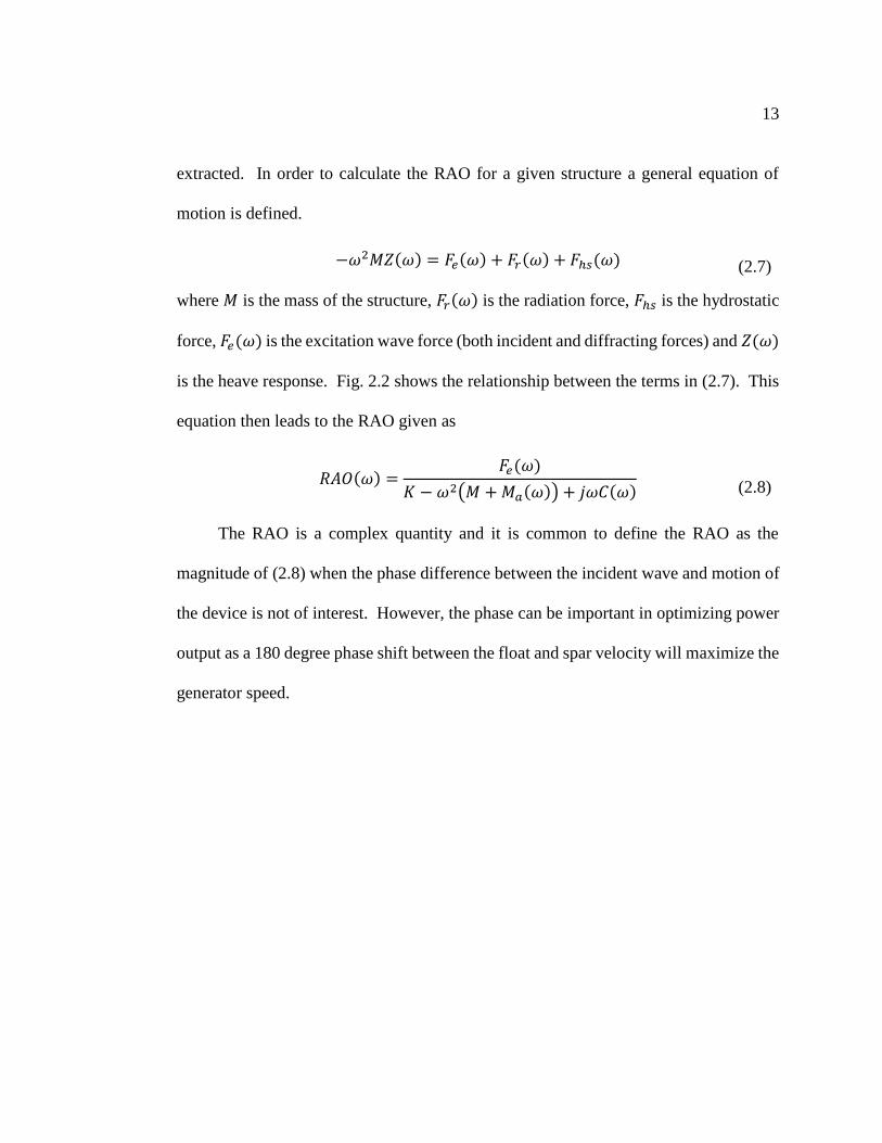
extracted. In order to calculate the RAO for a given structure a general equation of
motion is defined.
−𝜔2𝑀𝑍(𝜔) = 𝐹𝑒(𝜔) + 𝐹𝑟(𝜔) + 𝐹ℎ𝑠(𝜔) (2.7)
where 𝑀 is the mass of the structure, 𝐹𝑟(𝜔) is the radiation force, 𝐹ℎ𝑠 is the hydrostatic
force, 𝐹𝑒(𝜔) is the excitation wave force (both incident and diffracting forces) and 𝑍(𝜔)
is the heave response. Fig. 2.2 shows the relationship between the terms in (2.7). This
equation then leads to the RAO given as
𝑅𝐴𝑂(𝜔) =𝐹𝑒(𝜔)
𝐾 − 𝜔2(𝑀 + 𝑀𝑎(𝜔)) + 𝑗𝜔𝐶(𝜔)
(2.8)
The RAO is a complex quantity and it is common to define the RAO as the
magnitude of (2.8) when the phase difference between the incident wave and motion of
the device is not of interest. However, the phase can be important in optimizing power
output as a 180 degree phase shift between the float and spar velocity will maximize the
generator speed.
14
Fig. 2.2. Equation of motion terms of fluid forces on a structure.
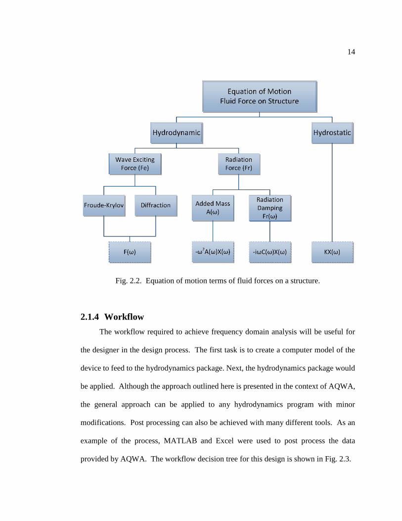
2.1.4 Workflow
The workflow required to achieve frequency domain analysis will be useful for
the designer in the design process. The first task is to create a computer model of the
device to feed to the hydrodynamics package. Next, the hydrodynamics package would
be applied. Although the approach outlined here is presented in the context of AQWA,
the general approach can be applied to any hydrodynamics program with minor
modifications. Post processing can also be achieved with many different tools. As an
example of the process, MATLAB and Excel were used to post process the data
provided by AQWA. The workflow decision tree for this design is shown in Fig. 2.3.
15
Fig. 2.3. Example workflow for frequency domain analysis.
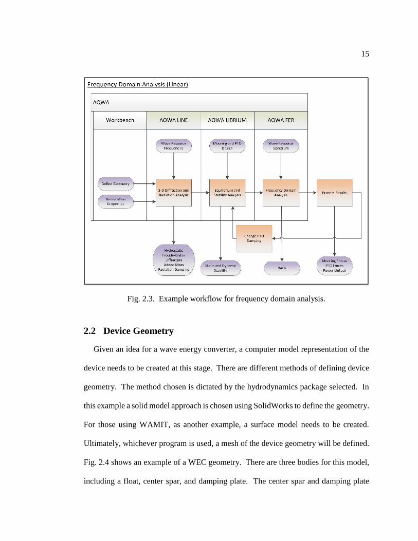
2.2 Device Geometry
Given an idea for a wave energy converter, a computer model representation of the
device needs to be created at this stage. There are different methods of defining device
geometry. The method chosen is dictated by the hydrodynamics package selected. In
this example a solid model approach is chosen using SolidWorks to define the geometry.
For those using WAMIT, as another example, a surface model needs to be created.
Ultimately, whichever program is used, a mesh of the device geometry will be defined.
Fig. 2.4 shows an example of a WEC geometry. There are three bodies for this model,
including a float, center spar, and damping plate. The center spar and damping plate

16
are locked together for the simulation. In a final design there would be a truss structure
between the spar and damper but for initial simulation this is ignored.
Fig. 2.4. Generic WEC example. A massless, stiff connection between the spar and
damper is present, but not shown. All dimensions in meters.

17
2.2.1 Solid Model
Once a concept for a design is developed, the first step in analysis is creating a
representation of the geometry of the device. This may take the form of a solid model,
surface model, etc. In this example a solid model was used. There are several modeling
packages available with which to develop a solid model. It is important to research the
geometric formats required by the hydrodynamic tool that shall be used.
Beyond providing a convenient user interface for developing a model, packages
such as SolidWorks can provide valuable information for model simulation such as the
center of gravity of bodies, inertia values associated with bodies, and mass properties.
As an alternative, many of the hydrodynamic software packages including ANSYS
AQWA provide a simple modeling platform sufficient for creating basic shapes and
devices.
Most WEC designs will be multi-bodied devices and in this case will be combined
as an assembly of parts. In the generic point absorber example a separate body was
created for the float, spar, and damper plate. The spar and damper are fixed together in
the hydrodynamics package and the only relative motion is between the float and
spar/damper. The reason for this has to do with the way that the hydrodynamic package
deals with the interface between two bodies. If the proximity of two bodies is small
enough, which is common in most WEC designs, the package requires time steps so
small that it is not practical to run the simulation. Therefore, for this model, there will
be three separate bodies, the float and damper plate will interact but there will be no
interaction between the spar and the float.

18
Once the solid bodies have been modeled, characteristics such as inertia values
and center of gravity can be gathered from the modeling program to be fed into the
hydrodynamics program. When the geometry is imported into the solid modeling
program the static water level needs to be defined and the body properties detailed. A
point mass is defined for each body with the inertia values specified.
A big part of the modeling process includes generating a mesh with which the
hydrodynamics program calculates the pressures and forces on each mesh element. This
is where a tradeoff between model accuracy and simulation time and storage space
needs to be made. Although a small mesh size would be preferred, a rougher mesh
provides significantly shorter simulation times and smaller output files. Depending on
the complexity of the bodies, and the patience for the simulation, a mesh size can be
determined. The larger mesh size that is chosen, the faster results are obtained, however
the smaller the mesh size, the more accurate the results will be. Take note that a single
mesh size does not have to be used. A finer mesh can and was used near the interface
between two bodies. This practice will lead to greater accuracy of results.
2.2.2 Mass Properties
Moments of inertia provide a measure of a bodies resistance to change in its state
of rotation. For example, in a hydrodynamic package such as AQWA, mass and inertia
values can be specified using a point mass approach. Inertia values can either be
specified directly or via knowledge of the radius of gyration. This is calculated as the
root mean square distance of the bodies parts from its center of gravity. SolidWorks
calculates inertia values for the bodies that can then be transferred to AQWA. By
19
default the mass definition is program controlled so there is no need to input mass
values. Alternatively, manually specifying the mass is an option.
The center of mass is the weighted average location of the mass of the body. For
example, the center of mass is communicated as an XYZ coordinate into AQWA for
each body. SolidWorks can be used to determine this center of mass using the mass
properties dialog. This allows for simplified calculations by the hydrodynamics
package by treating quantities as being referenced to the center of mass or treating a
body as if its entire mass is concentrated at the center of mass.
Significant thought should be given to where the center of mass is located in the
final design. For the device to be stable it needs to have a positive metacentric height.
The metacenter is calculated as the ratio of the inertia resistance of the device divided
by the volume of the device. At this stage however, device construction materials and
all components are most likely not known. Therefore caution should be used to ensure
that the center of mass is not in an unreasonable position.
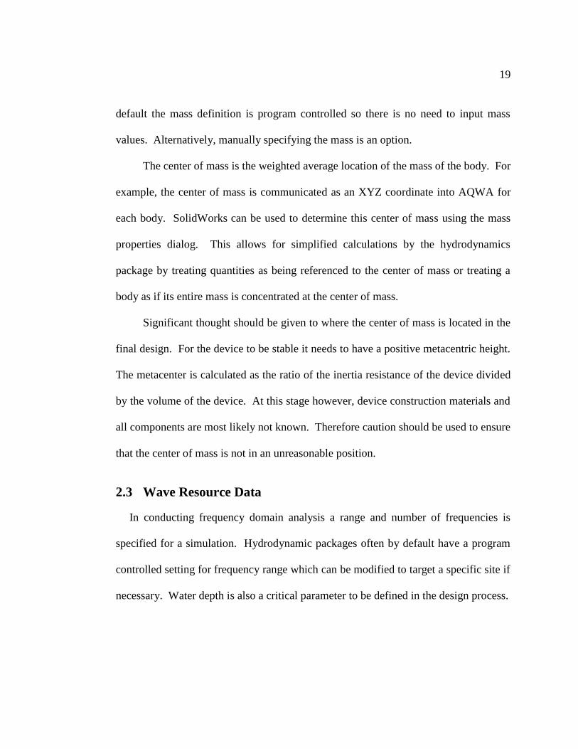
2.3 Wave Resource Data
In conducting frequency domain analysis a range and number of frequencies is
specified for a simulation. Hydrodynamic packages often by default have a program
controlled setting for frequency range which can be modified to target a specific site if
necessary. Water depth is also a critical parameter to be defined in the design process.

20
2.3.1 Range and Number of Frequencies
By default the range of frequencies may be program controlled by the
hydrodynamics package. This will provide a range that will include most if not all
conditions that the device might encounter. A total number of frequencies should also
be chosen where more frequencies provide more detailed results.
If one wishes to target a specific site with a targeted range of frequencies this is
possible. For example, the National Data Buoy Center (NDBC) [16] provides historical
data for many locations around the world. For example, if a site near the NDBC
Stonewall Banks buoy was chosen, historical data shows that a range of frequencies of
0.125 Hz to 0.3 Hz would capture the wave frequencies found at that site.
2.3.2 Wave Directions
Technically, if the device is symmetrical about the z-axis, there is no need to
calculate multiple incident wave angles. In practice, however more accurate results will
be obtained by choosing a number of incident wave angles. Increasing the number of
angles has a relatively small impact on simulation time. A wave range, interval, and
number of intermediate directions can be specified, all in degrees. For an asymmetrical
device this can be a critical degree of freedom which further complicates the analysis
results.
2.3.3 Water Depth
Water depth is a very important parameter in influencing power extraction of a
WEC device. Power output in shallow water can be different from that found in deep
water. From an analysis perspective, in general, a deep water assumption will make for
21
an easier process. However, if there is a desired location to target, or for specific scaled
testing conditions it is important to use the depth in which the device will operate. For
this example a deep water application was used with a depth of 1000 m.
2.4 Hydrodynamic Software Packages
There are several industry standard hydrodynamic codes available for analysis of
WECs. These include WAMIT [17], ANSYS AQWA, and Orcaflex to name a few.
There are also codes based on WAMIT such as WaveDyn and HydroD.
Both WAMIT and ANSYS AQWA solve the linear water wave boundary value
problem. They use the Boundary Element Method (BEM), also known as the panel
method and the integral method, to find diffraction and radiation velocity potentials. In
general, BEM apply source or dipole functions on the surfaces of submerged bodies,
and solve for their strength so that all boundary conditions are met [18]. Once the
diffraction and radiation velocity potential fields have been solved, excitation forces,
added mass and damping matrices, as well as wave field pressure, velocity, and surface
elevation can be found. Both WAMIT and AQWA can also find hydrostatic forces and
moments.
The primary difference between the two software packages is the data pre-
processing, post processing, software interface, and supplementary calculations.
WAMIT does not have a graphical user interface. Its inputs and outputs are text files
that require pre-processing and post-processing by another program. AQWA does have
a limited graphical interface that aids in part of the setup and analysis of a problem but

22
also uses text files for a significant portion of the modeling process. WAMIT users have
high level of control over setup and access to a wide range of data outputs. AQWA has
more post-processing computational tools including frequency domain analysis, time
domain analysis, and stability calculations.
In the end, at this stage, the excitation force, added mass matrix, damping matrix,
and hydrostatic coefficients need to be computed. Both WAMIT and AQWA compute
these values with the same technique. It is left to the user to decide which software
package is most comfortable, and whether additional data or analysis that is provided
by a specific tool is needed.
The current codes intended for WECs have been adapted from the ship industry
where ship dynamics have been studied. In general these vessels are much larger, single
bodied structures. Although improving, sometimes the application of these codes to
smaller, multiple bodies interacting, can lead to issues in convergence and accuracy.
This can be partially attributed to the nonlinear effects which have a greater influence
on the performance of the system at a smaller scale.
Hydrostatic results are also included in this stage. Center of gravity, volumetric
displacement, center of buoyancy, and metacentric heights are some of the parameters
available. These will help with keeping the proper stability of the device.
2.4.1 3-D Diffraction and Radiation Analysis
Once the solid model has been created and imported in the hydrodynamics
package, the first step in analysis is a 3-D diffraction and radiation analysis. This will

23
determine wave force and structure response calculations as well as hydrostatic analysis.
Outputs include the Froude-Krylov forces, diffraction forces, added mass, and damping
forces in the frequency domain as shown in Fig. 2.5.
Fig. 2.5. Example 3-D Diffraction and Radiation Analysis results.
Note, at this stage, there is no mooring or PTO defined and the structures are not
connected. This is acceptable for the device specific characteristics, namely the
hydrostatics, Froude-Krylov, added mass, and radiation parameters. However if we
would like to get information regarding the response amplitude operators, power
generation, or mooring characteristics we will have to run further analysis.
24
2.4.2 Equilibrium and Stability Analysis
Equilibrium and stability is the next step in the process. Static equilibrium and
stability of a system under the influence of the following steady forces: gravity,
buoyancy, wave drift force, steady wind force, current, thrusters, and mooring are
considered.
This is the stage where the mooring and power take off model gets introduced into
the system. Equilibrium and stability analysis is necessary to move on to both frequency
and time domain modeling.
2.4.3 Frequency Domain Analysis
Frequency domain response allows insight into the RAOs and relative velocity
measurements which lead to power output calculations based on power take off
implementation and mooring application. The hydrodynamic package calculates the
significant response of amplitudes in irregular waves. It utilizes a linearized stiffness
matrix and damping to obtain the transfer function and response spectrum. The major
benefit of this type of analysis is the ability to make a systematic parameter study while
getting power predictions for the device. At this stage, a mooring model and power take
off need to be defined to simulate a more complete system. The following sections
describe the models used.
2.4.4 Mooring Model (Linearized)
The mooring configuration used in this example is a three point system. The
lines are assumed to be a conventional linear elastic cable. The lines are assumed to
25
have no mass and geometrically are represented as a straight line. The stiffness and the
unstretched length are the two parameters that need to be specified.
Another option is a single point catenary mooring system. This can be modeled
as a composite elastic catenary with weight. Mass per unit length and equivalent cross
sectional area are properties that need to be defined for this type of mooring model.
There are many more possibilities for mooring a wave energy converter. The
importance of mooring design and modeling should not be overlooked. Reference [19]
shows many different mooring configurations with detailed analysis.
2.4.5 Power Take Off Model (Linearized)
One way to model a power take off (PTO) system is with an articulation allowing
rotational motion. For this articulation a rotational damping term can be specified.
Therefore, one must convert the rotational damping specified to an equivalent linear
damping value to calculate the PTO force. Once that conversion has been made,
calculating 𝐹𝑝𝑡𝑜becomes
𝐹𝑝𝑡𝑜(𝜔) = 𝑢𝑟𝑒𝑙(𝜔)𝐵𝑙 (2.9)
where 𝑢𝑟𝑒𝑙 is the relative velocity between bodies and 𝐵𝑙 is the linear damping value.
2.4.6 Response Amplitude Operators (RAOs)
The hydrodynamic package will provide a Response Amplitude Operator for each
body. A sample output RAO magnitude and phase plot is shown in Fig. 2.6. As the
plot shows the response drops off for waves with a period lower than around five
seconds.

26
For example, if a monochromatic wave with an amplitude of 1 m and a frequency
of 0.3 Hz is considered, the resulting heave motion of the float will have a magnitude
of approximately 0.65 m and a phase shift of approximately 8 deg.
Fig. 2.6. RAO amplitude and phase for each body.
2.5 Output Power Comparisons
Once the PTO forces are known the next natural step is to calculate the power output
of the device as a function of frequency for different damping values. The power for
each frequency was computed using the following equation
𝑃𝑃𝑇𝑂(𝜔) = 𝑢𝑟𝑒𝑙(𝜔) 𝐹𝑃𝑇𝑂(𝜔) (2.10)
27
where 𝑢𝑟𝑒𝑙 is the relative velocity between the float and the damper and 𝐹𝑃𝑇𝑂 is the force
applied to the power take off.
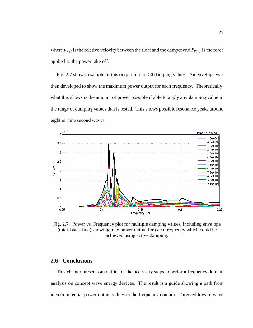
Fig. 2.7 shows a sample of this output run for 50 damping values. An envelope was
then developed to show the maximum power output for each frequency. Theoretically,
what this shows is the amount of power possible if able to apply any damping value in
the range of damping values that is tested. This shows possible resonance peaks around
eight or nine second waves.
Fig. 2.7. Power vs. Frequency plot for multiple damping values, including envelope
(thick black line) showing max power output for each frequency which could be
achieved using active damping.
2.6 Conclusions
This chapter presents an outline of the necessary steps to perform frequency domain
analysis on concept wave energy devices. The result is a guide showing a path from
idea to potential power output values in the frequency domain. Targeted toward wave

28
energy converter device developers, it provides a clear methodology from concept to
the first power predictions of a device.

29
3 Time Domain Analysis
3.1 Introduction
As the need for alternative energy sources increases, industries such as ocean wave
energy, promising utility scale power generation from a renewable source, continues to
grow. Wave Energy Converter (WEC) design is still in its infancy with significant
research being applied to new designs. Thus far, no topology has provided a clear
benefit over others in efficiency, cost of manufacture, maintenance requirements and
production, thus new devices continue to be developed [5]. This is unlike the wind
industry which has established a two or three blade horizontal axis wind turbine to be
the most cost effective and efficient.
A good overview of the Ocean Wave Energy field is given in [9]. Many papers on
the topic of time domain WEC modeling exist, including [20],[11],[10], but lack a clear
design methodology. An attempt at benchmarking devices exists in [13]. The work
presented in this document provides a clear time domain modeling approach of a
heaving point absorber which can be adapted to other types of devices. A block diagram
of the inputs and outputs of this stage is shown in Fig. 3.1.
3.1.1 Background
This document assumes that a rough physical WEC design has been chosen, and
frequency domain analysis has already been performed as outlined in [21]. This can be
achieved using any of the industry standard hydrodynamic software packages capable
of doing frequency domain analysis. The next step in the validation of the merits of the


31
3.1.2 Equations of Motion
The equations of motion can be obtained by summing the forces present on each
body. The total forces which act on the heave motion of the structures can be broken
down to many components. The excitation wave force, 𝐹𝑒(𝑡) is the summation of the
Froude-Krylov force and the diffraction force and is the force imparted on the device
by the incoming wave. The total radiation force, 𝐹𝑟(𝑡) is the force on the bodies due to
structure motion and can be decomposed into an added mass term and a radiation
damping term. The mooring force, 𝐹𝑚(𝑡) can be linearized or nonlinear, and can take
on many different configurations. The hydrostatic force, 𝐹ℎ𝑠(𝑡) is the force trying to
restore the structure to hydrostatic equilibrium. The PTO force, 𝐹𝑝𝑡𝑜 is the force
absorbed by the device to be converted to usable energy, and can be either linearized or
nonlinear. The general equation is as follows
𝑀�̈�(𝑡) = 𝐹𝑒(𝑡) + 𝐹𝑟(𝑡) + 𝐹ℎ𝑠(𝑡) + 𝐹𝑣(𝑡) + 𝐹𝑚(𝑡)
+ 𝐹𝑃𝑇𝑂(𝑡) (3.1)
as first introduced in [22] where 𝑀 is the mass of the body.
The excitation force, 𝐹𝑒(𝑡) can be computed as a convolution of the water surface
elevation and impulse response function from the frequency domain results obtained in
previous simulations
𝐹𝑒(𝑡) = ∫ 𝜂(𝜏)𝐹𝑡(𝑡 − 𝜏)𝑑𝜏∞
−∞
(3.2)
where 𝜂(𝑡) is the wave surface elevation at the WEC and

32
𝐹𝑡(𝑡) =1
2𝜋 ∫ 𝐹(𝜔)𝑒𝑗𝜔𝑡𝑑𝜔
∞
−∞
(3.3)
is the non-causal impulse response function of the heave mode, where 𝐹(𝜔) is the
frequency domain summation of the Froude-Krylov force and diffraction forces. This
presents a challenge because the excitation force at the current time is dependent on
future input values. This is partially due to the wave impacting a part of the device prior
to the wave impacting the point of analysis of the device as described in [23].
The radiation force, 𝐹𝑟(𝑡) can be computed as a convolution of the body velocity
and the radiation impulse response function combined with the contributing force of the
added mass at infinity of the body.
𝐹𝑟(𝑡) = − ∫ 𝑘(𝑡 − 𝜏)�̇�(𝜏)𝑑𝜏𝑡
−∞
− 𝑚(∞)�̈�(𝑡) (3.4)
where
𝑘(𝑡) =1
2𝜋 ∫ 𝐾(𝜔)𝑒𝑗𝜔𝑡𝑑𝜔
∞
−∞
(3.5)
as shown in [23]. The integral in (3.5) is guaranteed convergence by subtracting off the
added mass at infinity as shown in (3.6)
𝐾(𝜔) = 𝑅(𝜔) + 𝑖𝜔[𝑚(𝜔) − 𝑚(∞)] (3.6)
where 𝑅(𝜔) is the frequency domain radiation damping coefficients and 𝑚(𝜔) is the
added mass of the body. Reformulation of (3.1) by moving the 𝑚(∞)�̈�(𝑡) term to the
other side and defining 𝐹𝑟′ as
𝐹𝑟′(𝑡) = − ∫ 𝑘(𝑡 − 𝜏)�̇�(𝜏)𝑑𝜏𝑡
−∞
(3.7)
33
becomes
(𝑀 + 𝑚(∞))�̈�(𝑡)
= 𝐹𝑒(𝑡) + 𝐹𝑟′(𝑡) + 𝐹ℎ𝑠(𝑡) + 𝐹𝑣(𝑡) + 𝐹𝑚(𝑡)
+ 𝐹𝑃𝑇𝑂(𝑡)
(3.8)
𝐹ℎ𝑠 can be computed as the restoring force on the body attempting to bring it back
to equilibrium as follows
𝐹ℎ𝑠(𝑡) = 𝜌𝑔𝐴 𝑧(𝑡) (3.9)
where 𝜌 is the fluid density, 𝑔, is the acceleration of gravity, and 𝐴 is the water plane
surface area.
𝐹𝑣 is the viscous friction forces on the body. Typically these are considered to be
proportional to the velocity of the body and are determined experimentally.
𝐹𝑚 is the mooring force and can take many forms. Mooring configurations can be
very complicated and highly nonlinear. For this paper a simple catenary mooring is
considered in the form of a spring
𝐹𝑚(𝑡) = −𝐾𝑚𝑧(𝑡) (3.10)
where 𝐾𝑚 is the spring constant of the mooring.
3.2 Model to be Analyzed
For this research a generic two body point absorber was chosen as shown in Fig. 3.2.
It is assumed that a frequency domain analysis has already been performed as outlined
in [21]. Therefore the geometry has already been chosen and results from the frequency
domain analysis have already been obtained.

34
Fig. 3.2. Generic WEC example. All Dimensions in meters.
35
The pertinent frequency domain parameters needed for the time domain simulation
include the following.
The Froude Krylov plus diffraction frequency domain coefficients describing
the resulting forces on a body imparted by an incoming wave.
The radiation damping coefficients describing the motion of the body in a fluid,
generating outgoing waves in phase with the body velocity thus acting as a
velocity proportional damping force.
The added mass coefficients defined as the added inertia on a body undergoing
harmonic oscillation due to the presence of the surrounding fluid.
3.3 Input Waves
It is possible and insightful to simulate both regular (monochromatic) and irregular
(spectrum) waves in the time domain simulation. Regular waves give a controlled input
that is repeatable and the response for the given input easily identified. Irregular waves
provide a more realistic representation of what the WEC would face in real seas.
3.3.1 Regular Waves
For regular wave input, a sinusoidal (also called harmonic) linear wave can be
defined as shown in the following linear wave input.
𝜂(𝑡) = 𝐴𝑐𝑜𝑠(𝜔𝑡) (3.11)
where 𝜔 is the frequency in radians/sec, and 𝜂(𝑡) is the water surface elevation at the
WEC in meters.

36
3.3.2 Irregular Waves
For irregular wave input, typical wave spectra include Jonswap, Pierson-
Moskowitz, Bretschneider, and Gaussian, distribution [24]. These wave inputs are all
uni-directional. A typical treatment of the spectrum is as follows. The spectrum is split
into N sections of equal area. N wavelets with frequency at the centroid of the section
are defined with N having a maximum of 200. The wavelets are then added together
with random phase angles taking on the following form
𝜂(𝑡) = ∑ 𝑎𝑖 cos(𝜔𝑖𝑡 + 𝜙𝑖)
𝑁
𝑖=1
(3.12)
For an example of a Pierson-Moskowitz input the following need to be specified.
The wave direction, the range of frequencies to be included, the significant wave height,
zero crossing period, and a seed used to define the random seed for a wave spectrum
must be included. For simulation purposes the resulting time series can be input into
the simulation.
3.4 Time Domain Differential Equation Solver Approach
One method for modeling a two body wave energy converter is by using a solver to
solve the equations of motion and then calculate outputs from that simulation. These
equations of motion describe the motion of the individual bodies due to many forces as
shown in the introduction to this paper. The dominant forces which are present in an
actual wave energy converter model and will be outlined here. We are considering a
device with two bodies and therefore will have two equations of motion, one for each

37
body. Subscript 1 will refer to the float and subscript 2 will refer to the spar as shown
in Fig. 3.3.
Fig. 3.3. MATLAB/Simulink implementation of equations of motion for two body
WEC.
Additional forces include a viscous damping force, a power take off force, and
mooring forces. With the addition of these forces, the equations of motion in the heave
direction for each body take the form
38
𝐹𝑒1(𝑡) − 𝐹𝑟11′(𝑡) − 𝐹𝑟21′(𝑡) − 𝐹ℎ𝑠1(𝑡) − 𝐹𝑝𝑡𝑜(𝑡)
− 𝐹𝑣1(𝑡) = (𝑀1 + 𝑚1(∞))�̈�(𝑡) (3.13)
𝐹𝑒2(𝑡) − 𝐹𝑟22′(𝑡) − 𝐹𝑟12′(𝑡) − 𝐹ℎ𝑠2(𝑡) + 𝐹𝑝𝑡𝑜(𝑡)
− 𝐹𝑣2(𝑡) − 𝐹𝑚(𝑡) = (𝑀2 + 𝑚2(∞))�̈�(𝑡) (3.14)
where 𝐹𝑒1(𝑡) is the force imparted by the incoming wave on body 1, 𝐹𝑟11(𝑡) is the
radiation force imparted on body 1 as a result of the waves created by body 1, 𝐹𝑟21(𝑡)
is the radiation force imparted on body 1 as a result of the wave created by body 2,
𝐹ℎ𝑠1(𝑡) is the hydrostatic stiffness force on body 1, 𝐹𝑝𝑡𝑜(t) is the electromechanical force
on body 1 from the generator acting as the power take off, and 𝐹𝑣1(𝑡) is the force from
viscous friction on the body. The second equation takes the same form as the first with
the exception of the sign on the PTO force and the addition of the mooring force attached
to body 2.
These equations were then input into MATLAB/Simulink as shown in Fig. 3.3. Note
that there are two similar structures of computation, one for each body. The excitation
forces, radiation forces, and hydrostatic forces are calculated in subsystems which will
be detailed below.
The excitation force calculation 𝐹𝑒, as shown in equation (3.2), is shown in Fig. 3.4.
First the impulse response function is calculated by solving the integral as shown in
equation (3.3) using the parameters obtained by a software package such as ANSYS
AQWA[14] or WAMIT[17]. The resulting non-causal impulse response function is

39
then split into its causal part and non-causal part and convoluted with the wave surface
elevation 𝜂 as shown in equation (3.2). In Simulink, the convolution is implemented
using the finite impulse response filter block with the impulse response function parts
fed as coefficients.
Fig. 3.4. Excitation Force convolution.
Notice that the input waveform was broken into a causal and a non-causal part which
are convoluted separately and the results added together. Also notice that a rate limiter
was used to ease the excitation force into the simulation. This is necessary because of
the non-causal nature of the excitation force. The radiation force has a similar structure,
however as the impulse response function is causal in nature, it requires just one
convolution.
The most common and straight forward initial model for the power take off is as a
linear damping. Its implementation in the model becomes a constant damping gain that
is multiplied by the relative velocities between the two bodies which provides the power
take off force calculation. Although this is convenient and a relatively accurate and

40
effective control scheme for some regions of operation, introduction of nonlinear
damping parameters can both provide a more realistic model of the system and could
potentially improve the power output from the device.
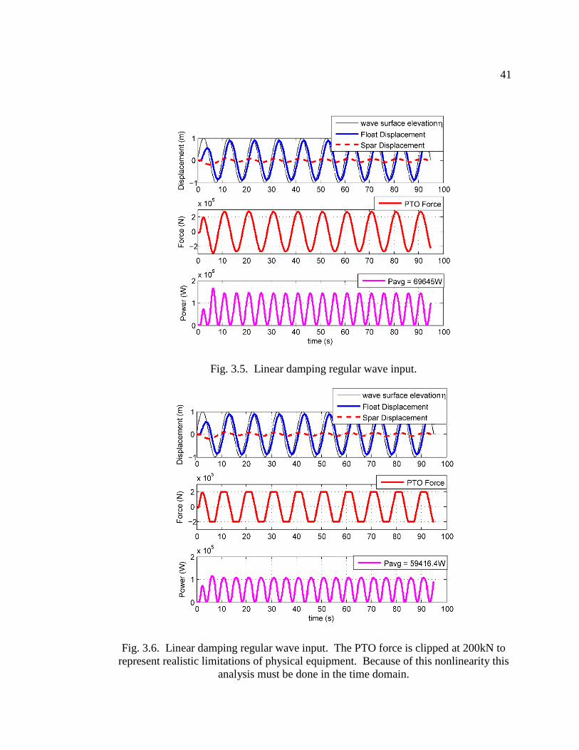
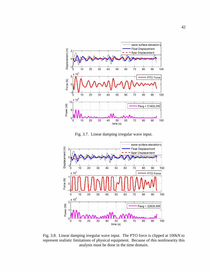
3.5 Simulation Results
Simulation of a two-body WEC was performed with both regular and irregular wave
inputs. Two different power take off damping schemes were employed for regular
waves. The first, linear damping produced a sinusoidal output in displacement, force,
and power, as expected and shown in Fig. 3.5. The second, saturated linear damping,
implemented limits on the damping applied and effectively clipped the force applied to
the power take off and thus the power produced as shown in Fig. 3.6. Due to this non-
linearity, this analysis cannot be done in the frequency domain.
The same set of damping conditions were then applied to an input of irregular sea
data as shown in Fig. 3.7 for linear damping and Fig. 3.8 for saturated linear damping
where the nonlinear clipping of the signal is clearly shown.
41
Fig. 3.5. Linear damping regular wave input.
Fig. 3.6. Linear damping regular wave input. The PTO force is clipped at 200kN to
represent realistic limitations of physical equipment. Because of this nonlinearity this
analysis must be done in the time domain.
42
Fig. 3.7. Linear damping irregular wave input.
Fig. 3.8. Linear damping irregular wave input. The PTO force is clipped at 100kN to
represent realistic limitations of physical equipment. Because of this nonlinearity this
analysis must be done in the time domain.

43
3.6 Conclusions
In this research, a methodology for modeling a two body point absorber wave energy
converter was outlined. The procedure included defining equations of motion and
implementing them in a differential equation solver such as MATLAB/Simulink. A
benefit of time domain simulation, namely the implementation of a nonlinear damping
power take off model, was analyzed and results shown. This demonstrates that time-
domain analysis, accommodating non-linearities in plant behavior or control, can be
conducted starting from frequency domain analysis.
44
4 Wave Tank Testing and Model Validation
4.1 Introduction
In order to fully realize a robust, efficient, and cost effective ocean wave energy
converter, considerable modeling and testing of devices will be required. Due to the
size and complexity of the full scale devices, the most cost effective way to make
advances is through the use of numerical modeling and scaled prototype testing. This
paper takes previous numerical modeling work and attempts to validate these models
with a scaled prototype tested in a large wave flume.
Wave tank testing of wave energy converters is a complicated endeavor with many
challenges. There is much to be learned from previous attempts at characterizing
devices and validating models. The European Marine Energy Centre (EMEC) provides
a tank testing standard in [24] and the University of Edinburgh has provided tank testing
guidance in [25]. The book edited by Joao Cruz [9], has a chapter dedicated to
numerical and experimental modeling of WECs which is quite insightful.
The main thrust of this research is to outline the process of taking an idea of a Wave
Energy Converter (WEC) and bringing it through the prototype stage of development.
This includes a significant amount of numerical modeling as well as physical modeling.
The outcomes of this chapter show the results of tank testing, namely the Response
Amplitude Operators (RAOs) and power performance results compared with two
different time domain model approaches. This model validation helps to identify the
regions of operation that can be reasonably modeled, allows for the adjustment of the

46
include a relatively simple geometry, many previous studies and built devices based on
this principal, and the robust nature of such a device.
4.2.1 Geometry
Full scale geometry design of the AWEC was outlined in [27], where coastal
United States locations were chosen to help inform the design. A target of 200 W
continuous power was chosen to meet the general electrical load of autonomous buoys.
A focus on a simple shape was pursued for reasons of cost and ease of manufacture as
well as ease of modeling.
A two body approach was chosen where the relative motion between the bodies
actuates the power take off. Because of limitations related to the scaled testing facility,
the need for additional stability within the system, and the shallow water depth of some
prospective sites, a damping plate was added. To add further stability, additional weight
was added to the bottom of the device and buoyancy was added as high up as possible.
This served to lower the center of gravity, while raising the center of buoyancy and thus
creating a more stable device. The final full scale equivalent, and actual fabricated
geometry is shown in Fig. 4.2.

47
(a) (b)
Fig. 4.2. Autonomous Wave Energy Converter: (a) Full Scale and (b) ¼ scale. All
dimensions in meters.
4.2.2 Scaling
To create the most realistic model of the full scale device, the largest scale factor
for the prototype was chosen. This was limited by what would reasonably fit in the
testing facilities. A near shore location with water depth of about 14 m -- a National
Oceanic and Atmospheric Administration (NOAA) buoy location off the coast of
Galveston, TX -- was used as a target location. The maximum water level in the
proposed test facility divided by the water depth at the proposed site led to a scaling
factor of four. That is to say that in terms of size, the target full scale device would be
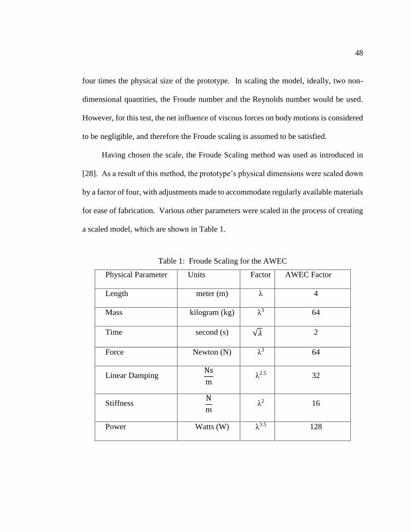
48
four times the physical size of the prototype. In scaling the model, ideally, two non-
dimensional quantities, the Froude number and the Reynolds number would be used.
However, for this test, the net influence of viscous forces on body motions is considered
to be negligible, and therefore the Froude scaling is assumed to be satisfied.
Having chosen the scale, the Froude Scaling method was used as introduced in
[28]. As a result of this method, the prototype’s physical dimensions were scaled down
by a factor of four, with adjustments made to accommodate regularly available materials
for ease of fabrication. Various other parameters were scaled in the process of creating
a scaled model, which are shown in Table 1.
Table 1: Froude Scaling for the AWEC
Physical Parameter Units Factor AWEC Factor
Length meter (m) λ 4
Mass kilogram (kg) λ3 64
Time second (s) √𝜆 2
Force Newton (N) λ3 64
Linear Damping Ns
m λ2.5 32
Stiffness N
m λ2 16
Power Watts (W) λ3.5 128

49
Of particular note is the scaling of power. The units of power are watts, also
written as
[𝑊] =[𝑘𝑔][𝑚]2
[𝑠]3
(4.1)
from the scaling table we see that the power scaling then becomes
𝜆3𝜆2
(√𝜆)3 = 𝜆3.5
(4.2)
so, from the target of 200 W continuous power and a scale factor of four the scaled
output power is 1.5625 W. Because of this large power scaling factor, extra care is
required to implement the scaled power take off system.
4.2.3 Power Take Off
The Power Take Off (PTO) system is responsible for converting the force created
by the motion of a WEC to some useful power. As is the case for a heaving point
absorber, this often requires the translation of linear motion to rotary motion. There are
many ways that this can occur including direct drive solutions as well as intermediate
energy translation solutions such as hydraulic systems. A study of direct drive solutions
is performed in [29]. A linear generator system is detailed in [30] and [31]. For the
project documented in this chapter, a ball screw spindle drive was chosen coupled to a
high efficiency brushed DC motor. At the scale of the built device this provided the
highest efficiency, lowest cost, and easiest implementation of readily available products.
For example, one beneficial aspect of this PTO device was the readily available drive

50
electronics consisting of a four quadrant servo-controller. This provided an easily
adaptable platform for the implementation of various control schemes.
4.2.4 Mooring
The mooring of wave energy conversion devices is very important and should not
be taken lightly. Mooring can significantly affect the power production, survivability,
environmental impact, and cost. An overview of a design approach is given in [32].
Mooring details for the scaled device is shown in section 4.4.3.
4.3 Linear Test Bed Testing
Due to the complex nature of a wave energy converter, there is a lot of useful
information that can be gleaned from testing before the device ever enters the water.
For this particular project the benefits of dry testing served two purposes. First, it
allowed for the testing of most system components in a situation similar to those it sees
in the water. Second, it allowed for the characterization of system losses, which are a
significant contributing factor affecting the performance of a device. These losses can
take many forms, but mostly can be attributed to friction, gearbox, and generator
inefficiencies. In an attempt to characterize the system losses, as well as do a complete
system validation, a Linear Test Bed (LTB) located in the Wallace Energy Systems and
Renewables Facility was used as shown in Fig. 4.3. An overview of the Linear Test
Bed is given in [33].
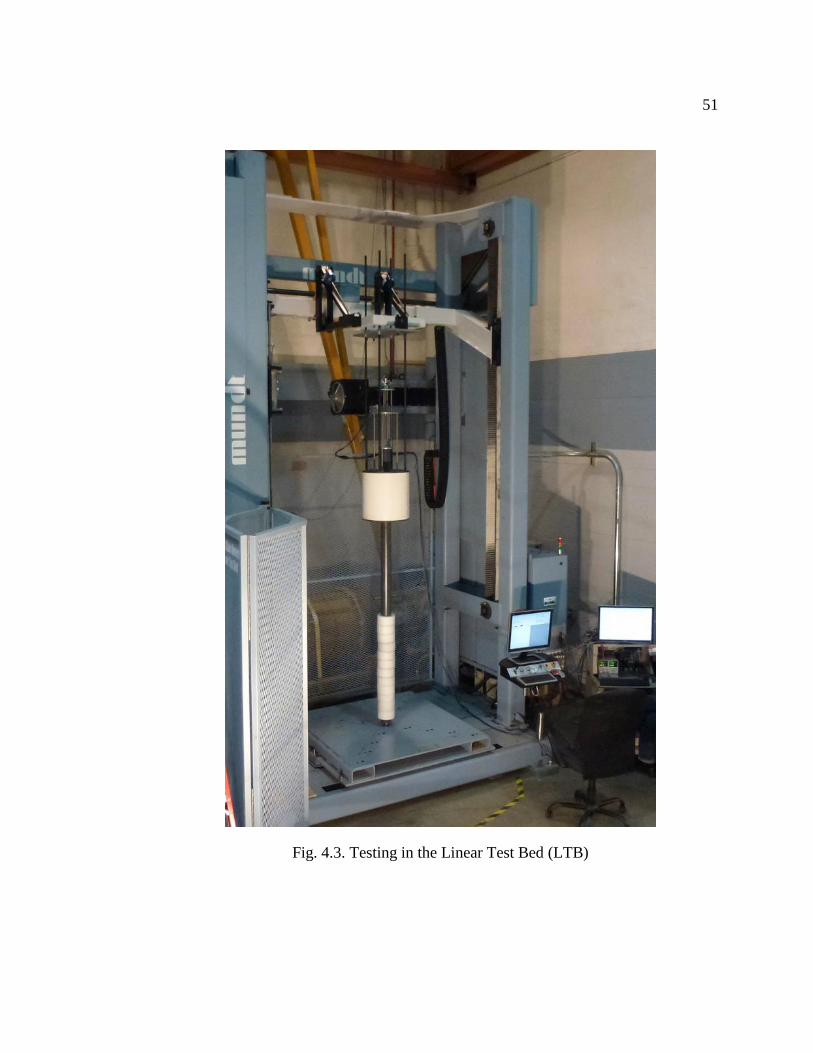
51
Fig. 4.3. Testing in the Linear Test Bed (LTB)
52
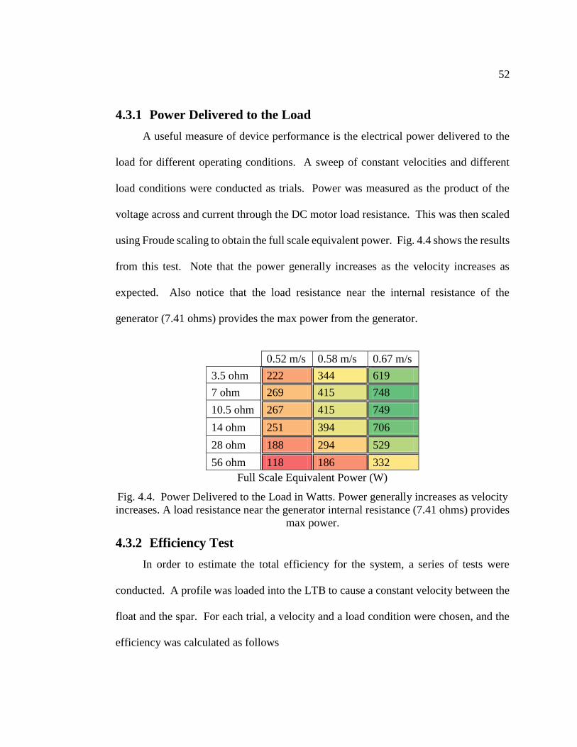
4.3.1 Power Delivered to the Load
A useful measure of device performance is the electrical power delivered to the
load for different operating conditions. A sweep of constant velocities and different
load conditions were conducted as trials. Power was measured as the product of the
voltage across and current through the DC motor load resistance. This was then scaled
using Froude scaling to obtain the full scale equivalent power. Fig. 4.4 shows the results
from this test. Note that the power generally increases as the velocity increases as
expected. Also notice that the load resistance near the internal resistance of the
generator (7.41 ohms) provides the max power from the generator.
0.52 m/s 0.58 m/s 0.67 m/s
3.5 ohm 222 344 619
7 ohm 269 415 748
10.5 ohm 267 415 749
14 ohm 251 394 706
28 ohm 188 294 529
56 ohm 118 186 332
Full Scale Equivalent Power (W)
Fig. 4.4. Power Delivered to the Load in Watts. Power generally increases as velocity
increases. A load resistance near the generator internal resistance (7.41 ohms) provides
max power.
4.3.2 Efficiency Test
In order to estimate the total efficiency for the system, a series of tests were
conducted. A profile was loaded into the LTB to cause a constant velocity between the
float and the spar. For each trial, a velocity and a load condition were chosen, and the
efficiency was calculated as follows

53
𝑃𝑖𝑛 = 𝑃𝑘 + 𝑃𝑟 + 𝑃𝑙𝑜𝑠𝑠 + 𝑃𝑒𝑙𝑒𝑐 (4.3)
𝑃𝑒𝑙𝑒𝑐 = 𝑉𝑔𝑒𝑛𝐼𝑔𝑒𝑛 (4.4)
where 𝑃𝑖𝑛 is the power input to the system by the LTB, 𝑃𝑘 is the rate of change of the
linear kinetic energy present in the system which is zero for a constant velocity, 𝑃𝑟 is
the rate of change of the rotational kinetic energy in the system which is zero for a
constant velocity, 𝑃𝑙𝑜𝑠𝑠 is the power losses in the system, and 𝑃𝑒𝑙𝑒𝑐 is the power
measured out of the generator.
𝑃𝑙𝑜𝑠𝑠 = 𝑃𝑖𝑛 − 𝑃𝑒𝑙𝑒𝑐 (4.5)
𝜂 =𝑃𝑒𝑙𝑒𝑐
𝑃𝑒𝑙𝑒𝑐 − 𝑃𝑙𝑜𝑠𝑠
(4.6)
where 𝜂 is the overall system efficiency.
Fig. 4.5 shows the results of these trials. Generally, as the speed increased, so did
the efficiency. Also, the efficiency peaks for the generator load at approximately double
the generator internal resistance (7.41 ohms).
0.52
m/s
0.58
m/s
0.67
m/s
3.5 ohm 15 16 22
7 ohm 21 23 32
10.5
ohm 23 25 41
14 ohm 26 27 39
28 ohm 22 22 47
56 ohm 13 14 29
Efficiency %
Fig. 4.5. Total PTO efficiency in % for different velocities and loads. As speed
increases, so does efficiency. The efficiency peaks for the generator load at
approximately twice the generator internal resistance (7.41 ohms).

54
4.3.3 Estimated Damping Values Due to Losses
In order to include the losses in any model of the overall system, an estimate of
those losses should be included. Although these losses are nonlinear, a linear damping
term is the easiest way to implement the estimated losses and is a good first pass
approximation. This term can be estimated as follows
𝐹𝑙𝑜𝑠𝑠 = 𝐵𝑙𝑜𝑠𝑠𝑣 (4.7)
𝑃𝑙𝑜𝑠𝑠 = 𝐹𝑙𝑜𝑠𝑠𝑣 = 𝐵𝑙𝑜𝑠𝑠𝑣2 (4.8)
𝐵𝑙𝑜𝑠𝑠 =𝑃𝑙𝑜𝑠𝑠
𝑣2
(4.9)
where 𝐹𝑙𝑜𝑠𝑠 is the equivalent loss force in the system; 𝐵𝑙𝑜𝑠𝑠 is the loss damping and
captures friction and other high order loss mechanisms; 𝑣 is the linear velocity; and 𝑃𝑙𝑜𝑠𝑠
is the power lost due to the inefficiencies of the system. Again, the velocity and load
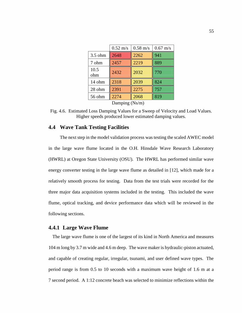
conditions were swept with the resulting estimates for 𝐵𝑙𝑜𝑠𝑠 shown in Fig. 4.6. As
expected, the higher speeds produced a lower estimated damping value. A mean value
of 2000 𝑁𝑠
𝑚 was used in both AQWA and MATLAB/Simulink full scale models.
55
0.52 m/s 0.58 m/s 0.67 m/s
3.5 ohm 2648 2262 941
7 ohm 2457 2219 889
10.5
ohm 2432 2032 770
14 ohm 2318 2039 824
28 ohm 2391 2275 757
56 ohm 2274 2068 819
Damping (Ns/m)
Fig. 4.6. Estimated Loss Damping Values for a Sweep of Velocity and Load Values.
Higher speeds produced lower estimated damping values.
4.4 Wave Tank Testing Facilities
The next step in the model validation process was testing the scaled AWEC model
in the large wave flume located in the O.H. Hinsdale Wave Research Laboratory
(HWRL) at Oregon State University (OSU). The HWRL has performed similar wave
energy converter testing in the large wave flume as detailed in [12], which made for a
relatively smooth process for testing. Data from the test trials were recorded for the
three major data acquisition systems included in the testing. This included the wave
flume, optical tracking, and device performance data which will be reviewed in the
following sections.
4.4.1 Large Wave Flume
The large wave flume is one of the largest of its kind in North America and measures
104 m long by 3.7 m wide and 4.6 m deep. The wave maker is hydraulic-piston actuated,
and capable of creating regular, irregular, tsunami, and user defined wave types. The
period range is from 0.5 to 10 seconds with a maximum wave height of 1.6 m at a
7 second period. A 1:12 concrete beach was selected to minimize reflections within the
56
tank. A water depth of 3.353 m was chosen as this was the maximum reasonable depth
for testing in the flume.
For the AWEC testing setup, several data acquisition measurements related to the
wave tank were included. A wave maker start signal, wave maker displacement, a wave
gauge located at the wave maker, and a pressure sensor level signal were all recorded.
Additionally, three resistance type self-calibrating wave gauges located near the tank
wall near the device under test were recorded. All signals were logged with a data
acquisition system with a sampling rate of 50 Hz. In the logging of data the goal is
typically to get the most accurate measure of the quantity desired with the smallest
amount of noise recorded. Because most of the frequencies of interest in the AWEC
model are much lower than most electrical noise, a low-pass filter is generally effective
in eliminating most of the noise from the acquired signal. Fig. 4.7 shows the basic
geometry and layout of the large wave flume, with the location of the wave gauges,
device under test (model AWEC), and optical tracking system (PhaseSpace).

57
Fig. 4.7. Large Wave Flume Configuration
4.4.2 Optical Motion Capture System
In attempting to validate numerical models of the AWEC system, it was very
important to have confidence in the motion tracking data of the bodies under test. A
PhaseSpace optical motion capture system was used for this purpose. This system,
designed for the entertainment industry, allows high resolution tracking of rigid bodies.
Twenty-seven uniquely identified active LED markers viewed by eight cameras
surrounding the device describe the PhaseSpace setup. Motion data is recorded at a 480
Hz sampling rate. Previous tests found a 6-sigma accuracy of 0.9 mm for all targets
within a 1.2 m radius, and 1.3 mm accuracy up to a 2.5 m radius [34]. Each body of the
AWEC was uniquely identified for six degrees of freedom in relation to the reference
coordinate definition square. Fig. 4.8 shows the PhaseSpace setup on the left and a
computer image showing the cameras and markers for each LED on the right.
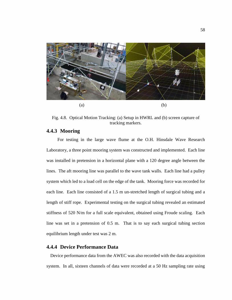
58
(a) (b)
Fig. 4.8. Optical Motion Tracking: (a) Setup in HWRL and (b) screen capture of
tracking markers.
4.4.3 Mooring
For testing in the large wave flume at the O.H. Hinsdale Wave Research
Laboratory, a three point mooring system was constructed and implemented. Each line
was installed in pretension in a horizontal plane with a 120 degree angle between the
lines. The aft mooring line was parallel to the wave tank walls. Each line had a pulley
system which led to a load cell on the edge of the tank. Mooring force was recorded for
each line. Each line consisted of a 1.5 m un-stretched length of surgical tubing and a
length of stiff rope. Experimental testing on the surgical tubing revealed an estimated
stiffness of 520 N/m for a full scale equivalent, obtained using Froude scaling. Each
line was set in a pretension of 0.5 m. That is to say each surgical tubing section
equilibrium length under test was 2 m.
4.4.4 Device Performance Data
Device performance data from the AWEC was also recorded with the data acquisition
system. In all, sixteen channels of data were recorded at a 50 Hz sampling rate using

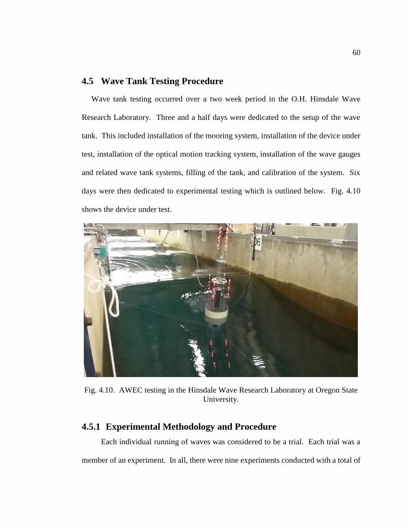
60
4.5 Wave Tank Testing Procedure
Wave tank testing occurred over a two week period in the O.H. Hinsdale Wave
Research Laboratory. Three and a half days were dedicated to the setup of the wave
tank. This included installation of the mooring system, installation of the device under
test, installation of the optical motion tracking system, installation of the wave gauges
and related wave tank systems, filling of the tank, and calibration of the system. Six
days were then dedicated to experimental testing which is outlined below. Fig. 4.10
shows the device under test.
Fig. 4.10. AWEC testing in the Hinsdale Wave Research Laboratory at Oregon State
University.
4.5.1 Experimental Methodology and Procedure
Each individual running of waves was considered to be a trial. Each trial was a
member of an experiment. In all, there were nine experiments conducted with a total of
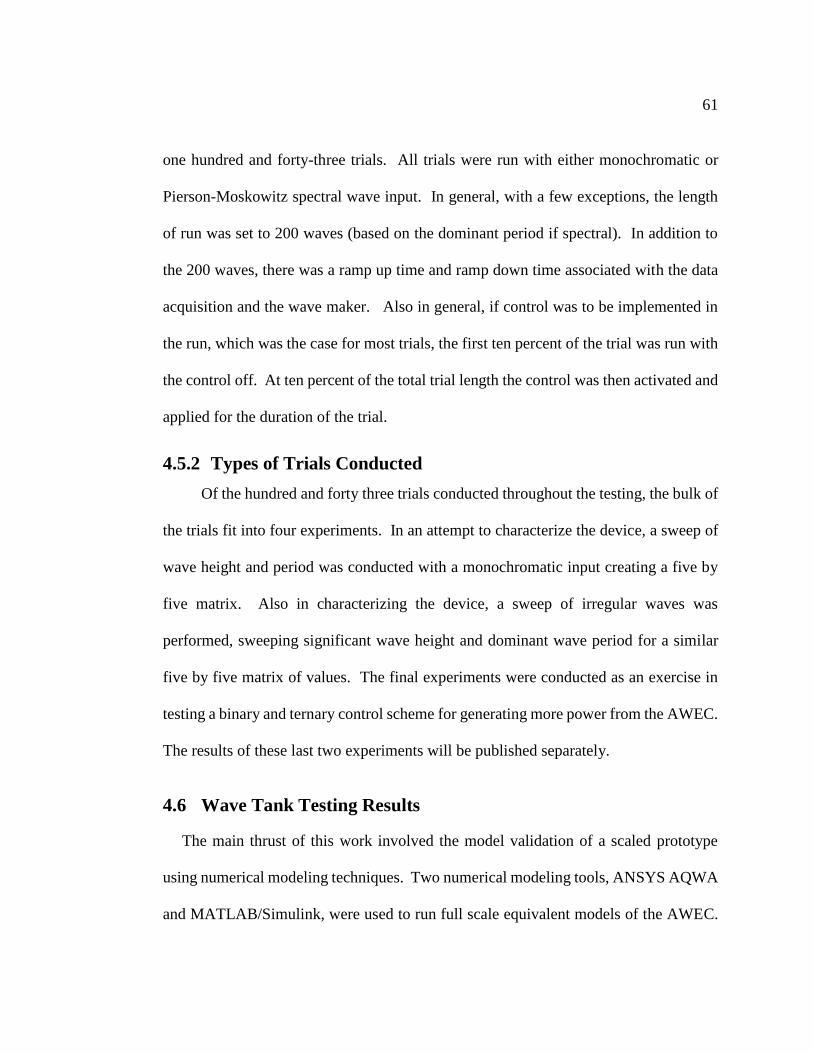
61
one hundred and forty-three trials. All trials were run with either monochromatic or
Pierson-Moskowitz spectral wave input. In general, with a few exceptions, the length
of run was set to 200 waves (based on the dominant period if spectral). In addition to
the 200 waves, there was a ramp up time and ramp down time associated with the data
acquisition and the wave maker. Also in general, if control was to be implemented in
the run, which was the case for most trials, the first ten percent of the trial was run with
the control off. At ten percent of the total trial length the control was then activated and
applied for the duration of the trial.
4.5.2 Types of Trials Conducted
Of the hundred and forty three trials conducted throughout the testing, the bulk of
the trials fit into four experiments. In an attempt to characterize the device, a sweep of
wave height and period was conducted with a monochromatic input creating a five by
five matrix. Also in characterizing the device, a sweep of irregular waves was
performed, sweeping significant wave height and dominant wave period for a similar
five by five matrix of values. The final experiments were conducted as an exercise in
testing a binary and ternary control scheme for generating more power from the AWEC.
The results of these last two experiments will be published separately.
4.6 Wave Tank Testing Results
The main thrust of this work involved the model validation of a scaled prototype
using numerical modeling techniques. Two numerical modeling tools, ANSYS AQWA
and MATLAB/Simulink, were used to run full scale equivalent models of the AWEC.

62
Results from the tank testing were scaled up for comparison with the numerical results
using Froude scaling. Because of the discrepancies between the commanded and
measured wave heights and periods, input to the numerical models were made to match
full scale equivalent measured wave tank wave heights and periods.
4.6.1 Commanded vs. Measured Wave Tank Results
For regular wave inputs wave gauge readings were taken on the wave maker side
of the AWEC. A desired period and wave height was given to the wave maker operator
for each trial. The resulting wave surface elevation was recorded at the location of the
wave gauge closest to the AWEC. All wave gauge data was filtered using a band-pass
Butterworth filter. The resulting measurement of the wave period closely matched the
expected period, however, the measured wave height deviated from the expected by as
much as 29%. Furthermore, for different periods given the same expected wave height,
the measured average wave height varied. Because of these results, all time domain
simulations done in both AQWA and MATLAB/Simulink received the scaled measured
input wave height in order to compare the theoretical results to measured results.
For irregular wave input, a similar process was followed. Because of restrictions
on the operation of the wave maker, two of the trials in the matrix were unable to be
completed. Results showed that there is significant error in both peak period and
significant wave height with a max error of 27% and 35% respectively. In order to
compare the hardware results with the numerical modeling, a scaled time series of
measured wave heights was used as the input to the AQWA and MATLAB/Simulink
numerical modeler.

63
4.6.2 Max Damping Value
For purposes of model validation and characterization of the system a fixed
damping value was needed in order to conduct the tests. In order to achieve a fixed
damping value the 4-quadrant drive was set in a current control (i.e., torque control)
operating mode. A velocity proportional damping term 𝐵 (𝑁𝑠
𝑚) was then used to set the
desired torque command to the motor. Early tests were run using a monochromatic
wave input to the system. As the trial progressed, after approximately every ten waves
the damping values were stepped up. Fig. 4.11 shows the results from a damping sweep
for two different monochromatic input waves, one with a full scale wave height of 1 m
and period of 4 s, and one with a full scale wave height of 2 m and period of 6 s. As the
plot shows the maximum full scale damping value for either case was near 𝐵 =
1600𝑁𝑠
𝑚, which was then chosen as the base damping value to be used for all sweeps of
wave height and period, both monochromatic and spectral.
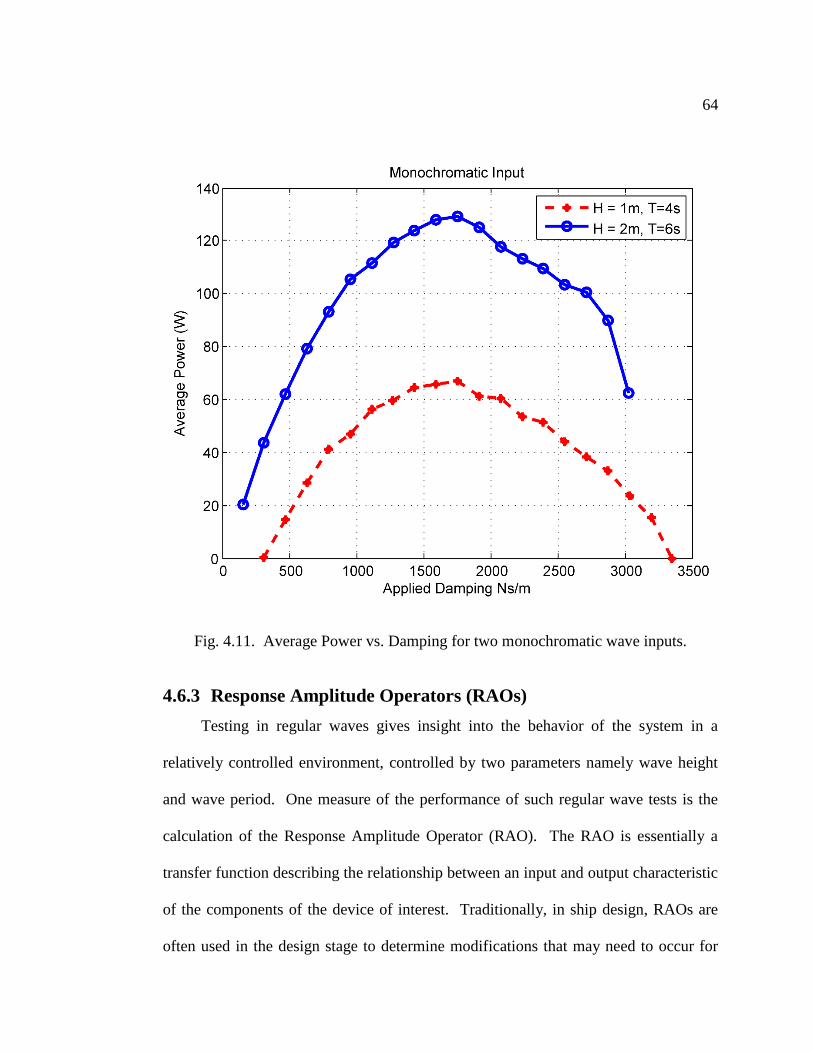
64
Fig. 4.11. Average Power vs. Damping for two monochromatic wave inputs.
4.6.3 Response Amplitude Operators (RAOs)
Testing in regular waves gives insight into the behavior of the system in a
relatively controlled environment, controlled by two parameters namely wave height
and wave period. One measure of the performance of such regular wave tests is the
calculation of the Response Amplitude Operator (RAO). The RAO is essentially a
transfer function describing the relationship between an input and output characteristic
of the components of the device of interest. Traditionally, in ship design, RAOs are
often used in the design stage to determine modifications that may need to occur for

65
safety reasons. In ocean wave energy conversion RAOs can be useful in design for
maximum power extraction. For this study, because of the nature of the point absorber,
the heave motion was identified as the pertinent motion for energy capture and thus the
RAO was calculated for each body, namely the float heave and spar heave as follows
𝑅𝐴𝑂 =𝜁
𝜂 [
𝑚
𝑚]
(4.10)
where 𝜁 is the body heave amplitude and 𝜂 is the incoming wave amplitude. For each
body the time series response was analyzed to find the positive zero crossings. Then
for each period the amplitude of the waveform was calculated. The average of these
values was then determined to be the body average heave amplitude. A similar process
was used to obtain the average incoming wave amplitude.
As part of the model validation process, three sets of RAOs were calculated and
compared for each rigid body. First, the tank test results of wave surface elevation as
measured by the resistance wave gauges was used with the optical motion tracking
information from PhaseSpace for the heave amplitude of each body. Second, time
domain simulations from ANSYS AQWA-NAUT were used to calculate the RAO.
Third, a MATLAB/Simulink time domain simulator based on the ANSYS AQWA
LINE hydrodynamic frequency domain parameters was conducted. The methodology
and a review of this modeling process is outlined in [21]. The RAOs for the three data
sets are shown in Fig. 4.12.
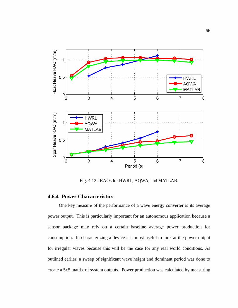
66
Fig. 4.12. RAOs for HWRL, AQWA, and MATLAB.
4.6.4 Power Characteristics
One key measure of the performance of a wave energy converter is its average
power output. This is particularly important for an autonomous application because a
sensor package may rely on a certain baseline average power production for
consumption. In characterizing a device it is most useful to look at the power output
for irregular waves because this will be the case for any real world conditions. As
outlined earlier, a sweep of significant wave height and dominant period was done to
create a 5x5 matrix of system outputs. Power production was calculated by measuring

67
the bus voltage and the currents in the circuit and then calculating the power generated
by the PTO. The result is the total power produced including all losses. Time domain
simulations were then performed using ANSYS AQWA-NAUT and a time domain
simulation tool in MATLAB/Simulink developed by the author described in [35] in an
attempt to simulate the testing environment. As described earlier, the losses
implemented in the numerical models were estimated as additional damping in the
system. The result is a power matrix plot showing the average power output for different
combinations of significant wave height and dominant period irregular wave inputs for
one hardware test and two hydrodynamic modeling exercises as shown in Fig. 4.13.
(a) (b) (c)
Fig. 4.13. Power Matrix for Irregular wave input: (a) HWRL wave tank testing, (b)
AQWA model, and (c) MATLAB model.
In order to quantify the differences between the model and the measured data, the
percent error was calculated between the different methods. Fig. 4.14 shows the % error
between the measured data and AQWA simulated data. As shown, the match is quite
good at the nominal case. As lower significant wave heights and peak periods are
analyzed the error generally gets larger, with the AQWA model over-predicting the
power output of the system. As significant wave heights increase and peak periods
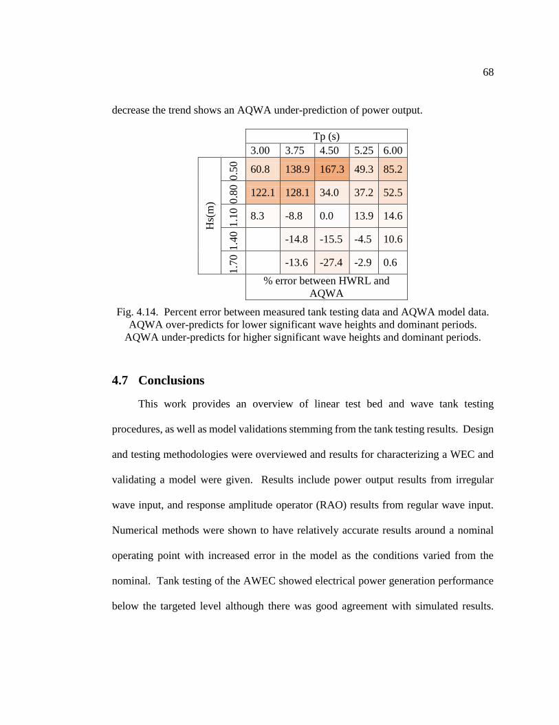
68
decrease the trend shows an AQWA under-prediction of power output.
Tp (s)
3.00 3.75 4.50 5.25 6.00
Hs(
m)
0.5
0
60.8 138.9 167.3 49.3 85.2
0.8
0
122.1 128.1 34.0 37.2 52.5
1.1
0
8.3 -8.8 0.0 13.9 14.6
1.4
0
-14.8 -15.5 -4.5 10.6 1.7
0
-13.6 -27.4 -2.9 0.6
% error between HWRL and
AQWA
Fig. 4.14. Percent error between measured tank testing data and AQWA model data.
AQWA over-predicts for lower significant wave heights and dominant periods.
AQWA under-predicts for higher significant wave heights and dominant periods.
4.7 Conclusions
This work provides an overview of linear test bed and wave tank testing
procedures, as well as model validations stemming from the tank testing results. Design
and testing methodologies were overviewed and results for characterizing a WEC and
validating a model were given. Results include power output results from irregular
wave input, and response amplitude operator (RAO) results from regular wave input.
Numerical methods were shown to have relatively accurate results around a nominal
operating point with increased error in the model as the conditions varied from the
nominal. Tank testing of the AWEC showed electrical power generation performance
below the targeted level although there was good agreement with simulated results.

69
Future work includes refinements to the hydrodynamic design and the PTO system to
improve power generation.
70
5 Conclusion
A design and testing methodology for the development of ocean wave energy
converters has been developed and implemented. Initial modeling was conducted on a
full scale utility sized WEC. Wave tank testing was conducted on a one quarter scale
autonomous device and model validation was performed.
The first step in the process was the frequency domain analysis, where a general
sense of the system performance was gathered. ANSYS AQWA was used to obtain the
results. Results of RAOs and power as a function of frequency were presented as well
as the hydrodynamic properties of the device. This would allow for relatively fast shape
optimization.
Next, a time domain model was developed using MALTAB/Simulink. This model
is based on the results from the frequency domain. Non-linearities were introduced into
the model of the power take off, which were not possible in the frequency domain. This
provided a more realistic look at the system outputs.
Finally, a scaled prototype of an Autonomous Wave Energy Converter (AWEC)
was designed, built, and tested. Both frequency domain and time domain numerical
simulations were used to model the AWEC. Testing of the physical prototype was
conducted both in the Wallace Energy Systems and Renewables Facility (WESRF) and
the O.H. Hinsdale Wave Research Laboratory (HWRL), both located at Oregon State
University. Results showed reasonable agreement between the time domain modeling
and wave tank testing results near a nominal operating point.

71
5.1 Recommendation for Future Work
There are many directions that future work could go from this project. A very rich
data set was gathered during the hardware testing and much more analysis could be
performed on this data. One example is the mooring load cell data, which could be used
to modify and enhance the numerical mooring model. Other further improvements to
the numerical model could be implemented to strengthen the match with hardware. A
more complex model of losses in the system including the power take off system could
be beneficial. Introduction of nonlinear elements in the mooring time domain model
would also be an improvement. The physical prototype could then be put back onto the
linear test bed and conditions could be run to match the wave tank testing to further
validate the numerical model.
Another opportunity for future work could be additional tests run with the same or
modified hardware. The physical hardware from the test is in good condition and would
be ready for future testing. Small improvements, for example in the mechanical
bushings, could result in higher efficiencies for future tests. These bushings could be
replaced with some sort of bearing to help reduce losses. Also, the surface between the
spar and float could be investigated for a more appropriate system to reduce losses.
More complex control algorithms could also be explored using the existing hardware.
Improvements in the hydrodynamic design and PTO design could also significantly
improve power generation.

72
6 Bibliography
[1] “IEA - Publication:- Key World Energy Statistics 2012.” [Online]. Available:
http://iea.org/publications/freepublications/publication/name,31287,en.html.
[Accessed: 21-Jun-2013].
[2] A. Clément, P. McCullen, A. Falcão, A. Fiorentino, F. Gardner, K. Hammarlund,
G. Lemonis, T. Lewis, K. Nielsen, S. Petroncini, M.-T. Pontes, P. Schild, B.-O.
Sjöström, H. C. Sørensen, and T. Thorpe, “Wave energy in Europe: current status
and perspectives,” Renewable and Sustainable Energy Reviews, vol. 6, no. 5, pp.
405–431, Oct. 2002.
[3] S. H. Salter, “Wave power,” Nature, vol. 249, no. 5459, pp. 720–724, Jun. 1974.
[4] Paul T. Jacobson, George Hagerman, and George Scott, “Mapping and
Assessment of the United States Ocean Wave Energy Resource,”
DOE/GO/18173-1, 1060943, Dec. 2011.
[5] A. F. de O. Falcão, “Wave energy utilization: A review of the technologies,”
Renewable and Sustainable Energy Reviews, vol. 14, no. 3, pp. 899–918, Apr.
2010.
[6] “Commercialization Program | Oregon Wave Energy Trust.” [Online]. Available:
http://www.oregonwave.org/commercialization-program/. [Accessed: 22-Jun-
2013].
[7] J. Falnes, Ocean waves and oscillating systems : linear interactions including
wave-energy extraction. Cambridge: Cambridge University Press, 2005.
[8] M. McCormick, Ocean engineering mechanics : with applications.
Cambridge ;;New York: Cambridge University Press, 2010.
[9] J. Cruz, Ocean Wave Energy: Current Status and Future Prespectives, 1st ed.
Springer, 2008.
[10] K. Ruehl, T. K. A. Brekken, B. Bosma, and R. Paasch, “Large-scale ocean wave
energy plant modeling,” in Innovative Technologies for an Efficient and Reliable
Electricity Supply (CITRES), 2010 IEEE Conference on, 2010, pp. 379–386.
[11] Eidsmoen, “Simulation of a slack-moored heaving-buoy wave-energy converter
with phase control,” Division of Physics, Norwegian University of Science and
Technology, 1996.
[12] K. Rhinefrank, A. Schacher, J. Prudell, E. Hammagren, Z. Zhang, C. Stillinger,
T. Brekken, A. von Jouanne, and S. Yim, “Development of a Novel 1:7 Scale
73
Wave Energy Converter,” ASME Conf. Proc., vol. 2011, no. 44373, pp. 935–944,
Jan. 2011.
[13] A. Babarit, J. Hals, M. J. Muliawan, A. Kurniawan, T. Moan, and J. Krokstad,
“Numerical benchmarking study of a selection of wave energy converters,”
Renewable Energy, vol. 41, pp. 44–63, May 2012.
[14] “ANSYS Aqwa.” [Online]. Available:
http://www.ansys.com/Products/Other+Products/ANSYS+Aqwa. [Accessed: 01-
Jun-2012].
[15] “3D CAD Design Software SolidWorks.” [Online]. Available:
http://www.solidworks.com/. [Accessed: 13-Jun-2012].
[16] N. O. and A. A. US Department of Commerce, “National Data Buoy Center.”
[Online]. Available: http://www.ndbc.noaa.gov/. [Accessed: 25-Jun-2012].
[17] “Wamit, Inc. - The State of the Art in Wave Interaction Analysis.” [Online].
Available: http://www.wamit.com/. [Accessed: 01-Jun-2012].
[18] C. C. Mei, “Numerical Methods in Water-Wave Diffraction and Radiation,”
Annual Review of Fluid Mechanics, vol. 10, no. 1, pp. 393–416, 1978.
[19] J. Fitzgerald and L. Bergdahl, “Including moorings in the assessment of a generic
offshore wave energy converter: A frequency domain approach,” Marine
Structures, vol. 21, no. 1, pp. 23–46, Jan. 2008.
[20] V. Gomez, R. Guanche, C. Vidal, and I. Eguinoa, “Numerical simulation of a
submerged wave energy converter under irregular wave conditions,” in
OCEANS, 2011 IEEE - Spain, 2011, pp. 1 –10.
[21] B. Bosma, Z. Zhang, T. K. A. Brekken, H. T. Ozkan-Haller, C. McNatt, and S.
C. Yim, “Wave energy converter modeling in the frequency domain: A design
guide,” in 2012 IEEE Energy Conversion Congress and Exposition (ECCE),
2012, pp. 2099 –2106.
[22] W. Cummins, “The impulse response function and ship motions,” Schiffstechnik,
vol. 9, pp. 101–109, 1962.
[23] J. Falnes, Ocean waves and oscillating systems: linear interactions including
wave-energy extraction. Cambridge University Press, 2002.
[24] “Tank Testing of Wave Energy Conversion Systems : EMEC: European Marine
Energy Centre.” [Online]. Available: http://www.emec.org.uk/tank-testing-of-
wave-energy-conversion-systems/. [Accessed: 03-Dec-2012].
74
[25] G. Payne and D. Ingram, “Best practice guidelines for tank testing of wave
energy converters,” The Journal of Ocean Technology, vol. 4/4, pp. 38–70, 2009.
[26] P. Hart, “ONT – June 2012 : Autonomous Powerbuoys: Wave Energy Converters
As Power Sources For The Next Generation Of Ocean Observatories.” [Online].
Available: http://virtual.ocean-
news.com/article/Autonomous_Powerbuoys%3A_Wave_Energy_Converters_As
_Power_Sources_For_The_Next_Generation_Of_Ocean_Observatories/1081385
/114319/article.html. [Accessed: 09-May-2013].
[27] T. M. Lewis, A. von Jouanne, and T. K. A. Brekken, “Modeling and control of a
slack-moored two-body wave energy converter with finite element analysis,” in
2012 IEEE Energy Conversion Congress and Exposition (ECCE), 2012, pp. 938–
945.
[28] J. Newman, Marine hydrodynamics. MIT Press, 1977.
[29] K. Rhinefrank, A. Schacher, J. Prudell, T. K. A. Brekken, C. Stillinger, J. Z. Yen,
S. G. Ernst, A. von Jouanne, E. Amon, R. Paasch, A. Brown, and A. Yokochi,
“Comparison of Direct-Drive Power Takeoff Systems for Ocean Wave Energy
Applications,” IEEE Journal of Oceanic Engineering, vol. 37, no. 1, pp. 35 –44,
Jan. 2012.
[30] C. Bostrom, R. Waters, E. Lejerskog, O. Svensson, M. Stalberg, E. Stromstedt,
and M. Leijon, “Study of a Wave Energy Converter Connected to a Nonlinear
Load,” IEEE Journal of Oceanic Engineering, vol. 34, no. 2, pp. 123–127, 2009.
[31] C. Bostrom, B. Ekergard, R. Waters, M. Eriksson, and M. Leijon, “Linear
Generator Connected to a Resonance-Rectifier Circuit,” IEEE Journal of
Oceanic Engineering, vol. 38, no. 2, pp. 255–262, 2013.
[32] L. Johanning, G. H. Smith, and J. Wolfram, “Mooring design approach for wave
energy converters,” Proceedings of the Institution of Mechanical Engineers, Part
M: Journal of Engineering for the Maritime Environment, vol. 220, no. 4, pp.
159–174, Dec. 2006.
[33] P. M. (Peter M. Hogan, “A linear test bed for characterizing the performance of
ocean wave energy converters,” Thesis, 2007.
[34] K. Rhinefrank, A. Schacher, J. Prudell, E. Hammagren, C. Stillinger, D. Naviaux,
T. Brekken, and A. von Jouanne, “Scaled wave energy device performance
evaluation through high resolution wave tank testing,” in OCEANS 2010, 2010,
pp. 1–6.

75
[35] B. Bosma, T. Brekken, H. T. Ozkan-Haller, and S. C. Yim, “Wave Energy
Converter Modeling in the Time Domain: A Design Guide,” in IEEE Conference
on Technologies for Sustainability, Portland, OR, 2013.