On The Design of Fault Tolerant VLSI and WSINon-Homogenous Multipipelines

A Thesis Presented

by

Hussain Said Al-Asaad

to

The Department of Electrical and Computer Engineering

in partial fulfillment of the requirements

for the degree of

Master of Science

in the field of

Electrical and Computer Engineering

Northeastern University

Boston, Massachusetts

September 24, 1993

NORTHEASTERN UNIVERSITY

Graduate School of Engineering

Thesis Title: On The Design of Fault Tolerant VLSI and WSI Non-

Homogenous Multipipelines.

Author : Hussain Said Al-Asaad

Department : Electrical and Computer Engineering

Approved for Thesis Requirement of the Master of Science Degree

_______________________________ ____________Prof. James Feldman DateThesis Advisor

________________________________ ____________Prof. Mankuan Vai DateThesis Co-advisor

_______________________________ ____________Prof. Edward Czeck DateThesis Reader

________________________________ ____________Prof. John Proakis DateChairman of Department

Graduate School Notified of Acceptance:

_______________________________ ____________Dean Yaman Yener DateDirector, Graduate School

Contents

1 Introduction 1

1.1 Problem Statement 2

1.2 Thesis Overview 3

2 Background 5

2.1 Description of Multipipelines 5

2.2 Multipipeline Applications 7

2.2.1 Computers 7

2.2.2 Signal Processing 8

2.2.2.1 Bit serial Digital Signal Processing (DSP) arrays 8

2.2.2.2 DSP Transforms 9

2.2.3 Iterative cellular arithmetic arrays 10

2.3 Previous Work 10

2.3.1 Architecture 10

2.3.1.1 Switching elements 11

2.3.1.2 Switch Programming Logic 14

2.3.1.3 Testing circuitry 15

2.3.2 Diagnosis 16

i

2.3.3 Reconfiguration 18

2.3.4 Examples 21

2.4 Summary 22

3 New Design 24

3.1 Architecture 24

3.2 Implementation 25

3.3 Diagnosis 28

3.3.1 Distributed Diagnosis 28

3.3.2 Host Driven Diagnosis 29

3.3.2.1 Fault-Free Interconnections 29

3.3.2.2 Faulty Interconnections 30

3.4 Reconfiguration 32

3.4.1 Control 32

3.4.2 Algorithm 34

3.5 Examples 37

4 Simulation and Comparison 39

4.1 Simplicity 40

4.2 Efficiency 40

4.3 Area 41

4.4 Locality 42

4.5 Reliability Evaluation 42

ii

4.5.1 Markovian Modeling 43

4.5.2 Results 49

4.6 Effect of M and N 51

4.7 Summary 54

5 Concluding Remarks 55

5.1 Accomplishments 55

5.2 Future Research 56

Appendix A - The Turbo Pascal Code 58

A.1 Units Used 58

A.1.1 The Nodes Unit 58

A.1.2 The Plot Unit 62

A.2 The Transitional Fractions Programs 64

A.2.1 MAX's and MIN's transitional fractions 64

A.2.2 GUPTA's transitional fractions 67

A.2.3 HJM's transitional fractions 70

A.3 Reliability and MTTF Calculations 73

A.4 Yield and reconfiguration examples 75

A.4.1 GUPTA's Design 75

A.4.2 HJM's Design 80

Appendix B - Transitional Probabilities 88

iii

List of Figures

2.1 A general model of multipipelines. 6

2.2 A straight-through multipipeline. 6

2.3 A typical functional block diagram of a multipipelined vector supercomputer. 8

2.4 A multipipeline for serial DFT. 9

2.5 A popular architecture for multipipelines. 11

2.6 A multipipeline with a randomly distributed fault pattern. 11

2.7 A reconfigured multipipeline under the fault pattern of Figure 2.6. 11

2.8 The four modes (states) of the switch. 12

2.9 A CMOS circuit realizing the switching element using two control bits [2]. 13

2.10 A CMOS circuit realizing the switching element using three

control bits [5,8-9]. 13

2.11 The I/O to the Switch Programming Logic. 14

2.12 An example where a fictitious fault is created. 15

2.13 A simple boundary scan cell design. 16

2.14 The truth table of a SPL. 20

2.15 A reconfiguration example. 21

2.16 Length of interconnect depends on fault distribution. 22

3.1 The new architecture for the multipipeline. 24

3.2 The physical architecture for the multipipeline. 25

iv

3.3 The physical implementation of the multipipeline for the case of N is even. 27

3.4 Simple module structure. 28

3.5 The module structure under host driven diagnosis with fault-free

interconnections. 30

3.6 The module structure under host driven diagnosis with faulty

interconnections. 31

3.7 Reconfiguration signals between modules. 33

3.8 A reconfiguration example using Algorithm 3.1. 37

3.9 A reconfiguration example using Algorithm 3.2. 38

4.1 The expected number of survived pipelines normalized to the supplied

number of pipelines versus the fraction of faulty PEs. 41

4.2 The Markovian model for a 4×3 multipipeline. 43

4.3 General Markovian model for each state. 46

4.4 The transitional fractions in the Markovian model for a 3×3 multipipeline. 48

4.5 The reliability of an 8×8 HJM multipipeline with a stage failure rate of 0.1

failures per unit time. 49

4.6 The reliability of an 8×8 multipipeline with a PE failure rate of 0.1 failures

per unit time and with Sm = 2. 50

4.7 The reliability of an 8×8 multipipeline with a PE failure rate of 0.1 failures

per unit time and with Sm = 4. 50

4.8 The Mean Time to Failure in units of time of an 8×8 multipipeline with

a PE failure rateof 0.1 failures per unit time. 51

4.9 The fraction of survived pipelines for HJM design. 52

4.10 Expected yield (percentage of surviving pipelines) of an N×8 multipipeline. 53

v

B.1 The 3×3 multipipeline. 88

B.2 Reconfiguration in the three different cases of the faults locations. 90

vi

List of Tables

3.1 Values of FU and FD for different faults. 31

4.1 Comparison between the transitional fractions determined by simulation 48

and their corresponding exact values.

vii

Abstract

Multipipelines are currently used in many areas such as signal processing and

image processing architectures as well as in general purpose vector computers.

These pipelines are formed of several stages with different functionalities. The

main objective of the multipipelines design is to reduce the effects of faults by

having fault-tolerant design. In this thesis we present a new design for

multipipelines -- a new architecture, diagnosis, and reconfiguration algorithm.

The design is characterized by the unity length interconnect between the stages of

pipelines independent of the fault distribution, a low hardware overhead

compared to other designs, and a number of survived pipelines comparable to

other approaches.

viii

Chapter 1

Introduction

Multipipelines are often used to perform parallel pipelined operations with efficient

performance. They are currently spanning many areas from general purpose vector

supercomputers to application specific digital signal processing arrays.

Very large scale integration (VLSI) and wafer scale integration (WSI) technologies are

most advantageous when used to implement regularly structured systems such as large

arrays of identical processing elements. As integration level increases and the sizes of

arrays grow larger, the possibility of a single fault or multiple faults occurring in a VLSI or

WSI array increases. These faults can occur during the operational life time of an array, as

well as during its manufacturing process. If an array is not fault tolerant, the failure of a

single element can cause the entire array to fail completely. On the other hand, the array

might be able to operate in a fault-tolerant reconfigurable structure, where the array is

designed to tolerate some of the faults. This can be done by restructuring the array at

fabrication time to enhance the yield or by reconfiguring the array at run time to improve

reliability.

The reconfiguration problem of pipelines out of the structure in the presence of faults

has received much attention in the last years [1-9]. A distributed algorithm for this

purpose was described by [2]. The disadvantage of that algorithm is it can lead to

relatively long links between stages of the pipelines. This can decrease the performance

benefits of putting the pipelines on a single VLSI or WSI chip, since multipipelines are a

1

synchronous design where we must set the clock to accommodate the longest delay of

interconnections among stages. Furthermore, since we don't know a priori the length of

interconnections between the stages of the pipelines, we must implement all

interconnections with powerful buffers capable of driving the worst case path between

stages of the pipelines. This can impose very significant area, power, and delay penalties

on the design. Another disadvantage of the above algorithm is that it is not simple enough

to be implemented with little hardware and to be executed in a very short time.

On the other hand, it is possible to ensure at design time that the reconfigured

interconnections are probabilistically bounded [2,6]. The new approach presented in this

thesis is characterized by a constant interconnection length between stages independent of

the fault distribution. It is also characterized by its simplicity -- little hardware and time

overhead.

1.1 Problem Statement

The objective of designing a fault-tolerant multipipeline is to recover, in the presence

of faults, k pipelines out of N supplied ones. For example, if a vector processor uses at

least four pipelines and we supply eight of them, then a fatal failure is reached when five

out of the eight pipelines are faulty. The following issues arise in designing the fault-

tolerant multipipelines:

1- Architecture: The interconnection network between the columns of the

processing array should support fault-tolerant capabilities. It should be simple

enough so it does not add penalties on the array performance. Also, the

interconnection length between stages should be minimized.

2

2- Diagnosis: This corresponds to detecting defects/faults in both the network and

the processing elements. The diagnosis algorithm should be simple so the

testing hardware is kept at a minimal.

3- Reconfiguration: The reconfiguration algorithm should give a good harvest rate

and should have a minimal execution time. A simple algorithm is easy to

implement and it reconfigures the array in a short time.

The previous design of the multipipeline is characterized by a variable interconnection

length between stages dependent on the fault distribution, complex switching element that

forbids the assumption of fault-free switches, and a multi-phase sequential reconfiguration

algorithm. On the other hand, the new design presented in this thesis guarantees a constant

length of interconnect between stages independent of the fault distribution. The design

replaces the switching element by a simple two-input multiplexer, and has a parallel

distributed reconfiguration algorithm.

1.2 Thesis Overview

The thesis is organized as follows. In Chapter 2, the previous work in the area of fault-

tolerant multipipelines is discussed and their drawbacks are identified. The existing

reconfiguration algorithms and diagnosis are discussed in detail and a set of examples are

introduced to demonstrate their weaknesses. In Chapter 3, the new proposed architecture

as well as its implementation is described. The fault model assumed, the error diagnosis on

the new architecture, and the reconfiguration algorithms are also described in this chapter.

In Chapter 4, simulation is described in addition to comparison to previous approaches.

The comparison is performed from different points of view including simplicity, efficiency,

3

area, locality, and reliability. In Chapter 5, the main accomplishments are described and

the directions of future research are identified.

4

Chapter 2

Background

This chapter starts by describing multipipelines and their applications. Then, the

chapter describes the previous work in designing fault-tolerant multipipelines. This

chapter:

(1) Identifies the architectures used in multipipelines;

(2) Describes diagnosis methods on multipipelines;

(3) Describes reconfiguration algorithms found in the literature, and

(4) Identifies the weaknesses of the above.

2.1 Description of Multipipelines

A multipipeline is a set of identical pipelines each of which consists of several stages.

While an individual pipeline is obviously a linear array, the entire architecture can be seen

as a rectangular array with a simplified interconnection structure. Multipipelines can be

classified into two categories:

1- Homogeneous: All stages of the pipelines perform the same function, hence the

processing elements are perfectly identical, and a complete homogeneity of the

rectangular array exists. Although this case rarely happens, homogeneity can

exist at the expense of extra hardware.

2- Non-homogeneous: In this case the different stages of a single pipeline perform

different operations and the processing elements are therefore different. Thus

5

the multipipeline is not completely homogeneous, but homogeneity is found

column-wise.

Hereinafter, the term 'multipipeline' refers to non-homogeneous multipipelines. A

multipipeline is modeled as an array of processing elements (PEs) and is called an N×M

multipipeline. An N×M multipipeline is a set of N identical pipelines each consisting of M

stages. The stages are separated from each other by an interconnection network. A general

model of multipipelines is shown in Figure 2.1.

NETWORK

NETWORK

NETWORK

Figure 2.1 A general model of multipipelines.

The simplest form of the multipipeline is one which does not consider the fault

tolerance problem. An example of such a 3×4 multipipeline is shown in Figure 2.2.

Figure 2.2 A straight-through multipipeline.

As the connectivity of the interconnection network increases, the hardware required to

implement the network increases. This implies an increase in the probability of failure.

6

Hence, a tradeoff should be seeked between the simplest straight-through pipeline and one

with a fully connected interconnection network.

2.2 Multipipeline Applications

Multipipelines have a wide variety of applications which can be grouped into the

following areas: Computers, Signal processing, and Iterative cellular arithmetic arrays.

Each of these areas will be described in the next sections.

2.2.1 Computers

In supercomputers, multipipelines are often used to perform vector operations to

achieve efficient performance. The functional block diagram of a modern multiple-pipeline

vector computer [1] is shown in Figure 2.3. The instruction processing unit (IPU) fetches

and decodes scalar and vector instructions. Scalar instructions are forwarded to the scalar

processor for execution. The scalar processor itself contains multiple scalar pipelines.

After recognizing vector instructions by the IPU, the vector instruction controller takes

over in supervising its execution such as scheduling different instructions to different

multipipelines.

Although multipipelines are more popular in vector supercomputers, multipipelines are

also recently introduced in personal computers [20]. The new processor, PENTIUM, from

Intel has two independent integer pipelines which approximately double the performance

of the 80486 processor.

7

High

Speed

Main

Memory

InstructionProcessingUnit

ScalarRegisters

Vector

ControllerAccess

Vector

ControllerInstruction

VectorRegisters

Pipe 1

Pipe 2

Pipe n

Pipe 1

Pipe 2

Pipe m

ProcessorScalar

ProcessorVector

Figure 2.3 A typical functional block diagram of a multipipelined vector supercomputer.

2.2.2 Signal Processing

There are many applications of multipipelines to signal processing. These applications

include Bit serial digital signal processing (DSP) arrays and DSP transforms.

2.2.2.1 Bit serial Digital Signal Processing arrays

A typical interconnection structure found in DSP is the so called multi-row arrays as

shown in Figure 2.4. In some instances, all the pipelines are identical while individual

stages of a pipeline may be different. In other instances, the pipeline stages are identical. A

8

typical example of a circuit having exactly identical PEs is the convolver which performs

the function defined by:

Y k x j k w jj

N( ) ( , ). ( )= ∑

=

−

0

1

where x(j,k) is the jth input of the kth set, Y(k) is the output of the kth set, and w(j) are

fixed weights. Every pipeline j contains the corresponding fixed multiplicand w(j) and it

multiplies its input terms x(j,k) by this weight. The individual PEr of pipeline j contains the

fixed r-th bit of weight w(j), i.e., w(j,r). The cell r simply computes the partial product

x(j,k)×w(j,r) and adds it to the partial products generated by the other PEs of the pipeline.

The entire pipeline constitutes a serial multiplier implemented in a systolic way.

t1 t2

t2

t3

t3

t3

t4

t4

t4

t4

t5

t5

t5

t5

t6

t6

t6

w(0,0)

w(1,0)

w(2,0)

w(3,0)

w(0,1) w(0,2) w(0,3)Systolic Array of Multipliers

SystolicAdder

Y(0),Y(1), ...,Y(k)

w(1,1) w(1,2) w(1,3)

w(2,1) w(2,2) w(2,3)

w(3,1) w(3,2) w(3,3)

x(0,0)x(0,1)

x(1,0)

x(0,2)

x(1,1)

x(2,0)

x(0,3)

x(1,2)

x(2,1)

x(3,0)

x(2,k)

x(3,k-1)x(3,k)

x(0,k)

x(1,k-1)

x(2,k-2)

x(3,k-3)

x(1,k)

x(2,k-1)

x(3,k-2)

Input set number k

Direction of data flow

Figure 2.4 A multipipeline for serial DFT.

2.2.2.2 DSP Transforms

The flow graphs of DSP transforms can be mapped into multipipeline arrays to

increase throughput. Delays are inserted between stages to have the flow graph pipelined.

Some of these transforms are Fast Fourier Transform (FFT) and Fast Walsh-Hadamard

Transform (FWHT) [6].

9

2.2.3 Iterative cellular arithmetic arrays

These arrays use very small combinational cells to build highly parallel arithmetic

devices such as expandable multipliers and dividers. Since the cells are simple, the

overhead due to the interconnections added for fault-tolerant designs is not negligible.

Hence, an extremely simple design of the interconnections is favorable.

2.3 Previous Work

The previous work on fault tolerant multipipelines can be categorized into

architecture, diagnosis, and reconfiguration. Each of the following sections describe a

category of previous work on multipipelines.

2.3.1 Architecture

The popular designs for fault-tolerant multipipelines are described in [2,3,5,8,9]. A

multipipeline consists of several stages organized in rows and columns. The pipeline stages

are interleaved with switches for bypassing the faulty stages. This is shown for a 4×4

multipipeline in Figure 2.5. The switches are programmed according to the fault pattern to

increase the number of fault-free pipelines. A fault pattern of the 4×4 multipipeline is

shown in Figure 2.6. When this fault pattern happens in a non-fault tolerant design, all the

pipelines are faulty. While, by introducing the switches into the array, three out of the four

pipelines are recovered as shown in Figure 2.7.

The implementation of this architecture will require the understanding of the following

circuits: switching elements (SE), switch programming logic (SPL), and testing circuitry

(T). These components are described in the following sections.

10

Figure 2.5 A popular architecture for multipipelines.

Faulty Stage Healthy Stage

Figure 2.6 A multipipeline with a distributed fault pattern.

Figure 2.7 A reconfigured multipipeline under the fault pattern of Figure 2.6.

2.3.1.1 Switching elements

The function of a switching element is to connect its terminals according to a

predefined set of modes (states). The needed switching element has four states as shown

11

in Figure 2.8. Since the switch has four distinct states, two control bits (a and b) with

decoding are needed to choose a state. These two control bits are supplied by the switch

programming logic. A CMOS circuit that realizes a switch with these states is shown in

Figure 2.9 [2]. The circuit uses 10 transmission gates to connect its four terminals L, R, T,

and B.

00 01

10 11

00-mode

10-mode

01-mode

11-mode

T

B

L R

T

B

L R

T

B

L R

T

B

L R

Figure 2.8 The four modes (states) of the switch.

An alternative design uses three control bits (C1, C2, and C3) to eliminate the

decoding circuit. This design decreases the number of transmission gates used (6

transmission gates) at the expense of increased routing. As a result, the switch testing can

be done with less effort. The design of the switch using three control bits is shown in

Figure 2.10 [5,8-9].

12

L R

T

B

~a

a

a

a

aa

b

b

b

b

b

~b

~b

~b

~b

~b

~a

~a

~a

~a

Figure 2.9 A CMOS circuit realizing the switching element using two control bits [2].

L R

T

B

~C1

C1

C3~C3

~C2

C2

C1

~C1

C2

~C2

C3

~C3

Figure 2.10 A CMOS circuit realizing the switching element using threecontrol bits [5,8-9].

13

2.3.1.2 Switch Programming Logic

The switch programming logic (SPL) is responsible for programming the switches

according to the reconfiguration algorithm. A typical relationship between the SPL and

other array elements is shown in Figure 2.11. Its details will be described in the following

description.

SE(i,j)

SPL(i,j)

a b

LAR RAR

PE(i,j) PE(i,j+1)

T TLFF RFF

LF RF

Figure 2.11 The I/O to the Switch Programming Logic.

The SPL will be provided with:

- The status of left and right PEs whether they are faulty or healthy via

signals LF (left faulty) and RF (right faulty).

- Two signals from the SPL in the row above it indicating whether the SPL

in an earlier row wants a left or right PE. These signals are left adoption

request signal (LAR) and right adoption request signal (RAR).

On the basis of these signals and the reconfiguration algorithm, the SPL computes the

following six control signals:

(1) the control bits a and b for the switching element SE(i,j);

(2) the adoption requests for the SPL in the row below it;

14

(3) the fictitious fault signals left fictitious fault (LFF) and right fictitious fault

(RFF) for the left and right PEs respectively.

These fictitious signals are used for creating fictitious faults in the PEs. These PEs,

though healthy, cannot be utilized in building the fault free pipelines. Figure 2.12 shows an

example of a fictitious fault. In this case, either the PE "FF" or the one above it can be

used to form the upper pipeline. Once the upper one is selected, the PE "FF" is sacrificed

because we have a single track switch. Sacrificing the PE can be done by disabling the

testing circuit or the PE itself.

FF

FFFaulty PE Healthy PE Fictitious Fault

Figure 2.12 An example where a fictitious fault is created.

2.3.1.3 Testing circuit

The testing circuit (T) is responsible for providing the SPL with the status of the left

and right PEs. If the PEs are self-testing, then the circuit T may not be required. Another

alternative is to have an external tester which is responsible for providing the SPLs with

the test results. A fault in a PE results in that PE not included in any pipeline.

15

2.3.2 Diagnosis

Fault diagnosis is a perquisite for successful reconfiguration. Faults in the PEs are to

be located so they are not used in building the fault-free pipelines. On the other hand,

faults in switching elements need to be located down to the interconnection link or

transistor level to optimally utilize fault-free PEs. Fault diagnosis on a reconfigurable

multipipeline normally uses the boundary scan concept [8]. Boundary scan testing is a

technique that allows one to access all the primary inputs and outputs by connecting them

into a shift register. A simple boundary scan cell is shown in Figure 2.13. The flip flops of

all cells are connected together to form a large shift register with a single scan in port and

a single scan out port. This technique provides the internal test of each single PE as well

as an external test covering the interconnect between I/O pads on the board or a wafer. In

an internal test, i.e., a PE test, cells at the input pins of the PE apply the test patterns, and

those at the output pins of the PE capture the output responses. In an external test, i.e., an

interconnect test, cells at the output pins of the PEs in stage i are used to apply test

patterns, and those at the input pins of the PEs at stage i+1 capture the test responses.

MUX01

MUX01

Scan in

Scan out

Signal in Signal out

Mode control

ShiftClock

Flip flop

Figure 2.13 A simple boundary scan cell design.

16

Boundary scan is used in a way that the input and output registers in a PE can be

connected in a scan chain. All scan chains in the PEs of the same column can also be

connected into a longer scan chain. If each PE has distinct input and output registers, the

length of the chain is reduced by half by connecting them separately. In this case we have

two scan lines per column of PEs. On the other hand, all control registers in a column of

switch elements are connected into a shift register. Thus the switch setting information can

be shifted in through the chain.

Using the above scan design, it is evident that the PEs and switching elements can be

tested separately. A fault in the PE leads to avoiding the use of that PE in any pipeline and

hence it is no longer usable. A fatal fault in a switching element causes the number of

recoverable pipelines to decrease considerably. Thus in a switching element, the fault

needs to be located down to the level of a connection link or a transistor to optimally

utilize faulty switching elements.

This scan design supports the following modes of operation: normal, scan, and test

modes. In the normal mode of operation, the array performs its normal function. The scan

mode allows data to be shifted in or responses to be shifted out. The test mode can be

divided into two submodes: external and internal. Internal test provides a means of testing

the internal logic of the PEs. Test patterns are applied from the input register to the

internal logic in the PE. The corresponding responses are latched in the output register.

The results can be shifted out and verified. Internal test may include defective PE test and

the entire column test. Once a fault is detected in a column test, the individual PEs in the

column are tested to locate the faulty one. Various techniques can be developed for an

internal test depending on how test patterns are generated and how the responses are

verified.

The external test is to test the switching elements of the reconfigurable multipipelines.

The function of the switching element in the jth column of switches is tested by loading

17

test patterns into the output registers of the PEs in the jth column, applying them to the

switching elements, and capturing the test responses in the input registers in the (j+1) th

column. The responses can be shifted out and verified. The three bits of the switch control

registers should be set before applying the test patterns to the switching elements under

test. This information is shifted into the control bit registers since these registers are

connected in a chain. A fault in the switch control registers can be detected through the

path. Faults in switch control registers can be tolerated by providing redundancy in switch

control registers. In this way we need multiplexers to select between switch control

registers.

If there is no fault in the switching element, the switching element is reconfigurable to

any of the four switch states. If there is a fault in the switch, the switch might be able to

reconfigure to some of the states of the fault-free element. Thus in external testing, we

locate faults down to a connection link or a transistor to utilize a faulty element.

2.3.3 Reconfiguration

After locating the faults in the array, a reconfiguration of the array is performed. If the

diagnosis is distributed, then the PEs will have their status flip-flops continuously

reflecting their states. On the other hand, if the diagnosis is host driven, then the host will

perform the testing in the simplest form of a periodic basis in a semi-concurrent way.

An optimal algorithm -- an algorithm which finds the maximum number of pipelines --

is always favorable to the utilization of the hardware, but this should not be on the

expense of adding too much hardware or wasting too much time in executing the

algorithm.

An algorithm for programming the switches which does not take into account the

faults in the switches or interconnections is described in [2]. The algorithm works in

18

phases. At the beginning of each phase, each SPL tests the PEs surrounding it and samples

the left adoption request (LAR) and the right adoption request (RAR) signals sent by the

SPL above it. Based on this information, the SPL sets the switching element into the

appropriate state, generate the adoption signals to the SPL below it, and creates fictitious

faults if necessary.

The switches are programmed according to Figure 2.14. A "•" in the lower left (lower

right) corner indicates an adoption request for a left (right) PE. A "•" in the left (right)

side of the box indicates a fictitious fault created by the SPL to the left (right).

Each phase in the switch programming consists of setting rows of switches

sequentially, according to the table in Figure 2.14. N phases are required to extract as

many non-faulty pipelines as possible. In each phase, the top row of switches is first

programmed, which is then followed by the programming of the second row of switches,

and followed by the third row, and so on. This programming is done on the basis of the

permanent faults and the fictitious faults created in the previous phase. The

reconfiguration algorithm can be written as follows:

Algorithm 2.1

begindo N times {

for i=1 to N sequentially do∀j reset LAR (0,j) /* No adoption request */∀j reset RAR(0,j) /* for the first row */for j=1 to (M-1) in parallel do{

program the switch(i,j) according to Figure 2.14.}

}end

On the other hand, reconfiguring the array by taking care of faults in switches and

interconnects is currently under investigation by many researchers. The algorithm19

presented by [9] is characterized by its complexity, unoptimality, and the difficulty to be

implemented in a distributed way. Another algorithm based on finding the maximum flow

in a flow network is presented in [3] which is characterized by its optimality, complexity

(O(M×N)5/3), and the difficulty to be implemented in a distributed way. An optimal simple

distributed algorithm is a goal which has not been reached yet.

Switch ProgrammingAdoption Requests PE status SPL and PEs

LAR RAR Left Right After Programming

No No Good Good 00

No No Good Faulty 01 X

No No Faulty Good 10X

No No Faulty Faulty 00X X

No Yes Good Good 01

No Yes Good Faulty 00 X

No Yes Faulty Good 01X

No Yes Faulty Faulty 00X X

Yes No Good Good 10

Yes No Good Faulty 10 X

Yes No Faulty Good 00X

Yes No Faulty Faulty 00X XYes Yes Not Possible

Figure 2.14 The truth table of a SPL.

20

2.3.4 Examples

An example for reconfiguring multipipelines using Algorithm 2.1 is shown below in

Figure 2.15.

00 0100 X

01

X

00 01

X

X

01

01

10

10

10

00

Figure 2.15 A reconfiguration example.

Another example which shows that the length of the interconnection could become

many times longer than the fault-free case after a reconfiguration is shown in Figure 2.16.

In this figure, the switch in the first row is programmed to set the right adoption request to

the switch in the second row. The switch in the second (third) row is programmed to set

the right adoption request to the switch in the third (fourth) row and to create a fictitious

fault in the PE to the left of the switch. The switch in the fourth row is programmed in a

similar way to the switch in the first row. After programming the switches, the length of

the interconnect between the first stage in the first row and the second stage in the fourth

row is approximately four times the length of the fault-free case.

21

X

00

X

X

01

00

01

Figure 2.16 Length of interconnect depends on fault distribution.

2.4 Summary

The weaknesses of the multipipeline designs described in this chapter can be

summarized as follows:

1- The additional hardware to support reconfiguration is not small enough for

faults in that part of the hardware to be negligible.

2- The interconnections of the reconfigured multipipeline have lengths dependent

on the fault distribution. This leads to the slowing of the clock to

accommodate the worst case delay. So, the array performance is degraded.

3- No simple optimal distributed algorithm is known to us for reconfiguring the

array in the presence of faults in the PEs and switching elements.

4- The design presented in this chapter improves the yield in the manufacturing

phase as well as the reliability in the on-time phase. Thus, the design is general

22

to the point that it is not optimized for certain domain or application, which

leads to wasted resources.

23

Chapter 3

New Design

In this chapter a new design of fault tolerant multipipelines will be presented. A

detailed description will be given for this new architecture with issues in its

implementation, error diagnosis under different fault models, and reconfiguration

algorithms.

3.1 Architecture

A new architecture for a fault tolerant multipipelines is described in this thesis. The

emphasis is on its simplicity and a constant interconnection length between stages. Hence

the architecture shown in Figure 3.1 for 3×4 multipipeline is developed.

MUX

MUX

MUX

MUX

MUX

MUX

MUX

MUX

MUX

0,0

1,0

2,0

0,1

1,1

2,1

1,2

0,2

2,2

0,3

1,3

2,3

Figure 3.1 The new architecture for the multipipeline.

24

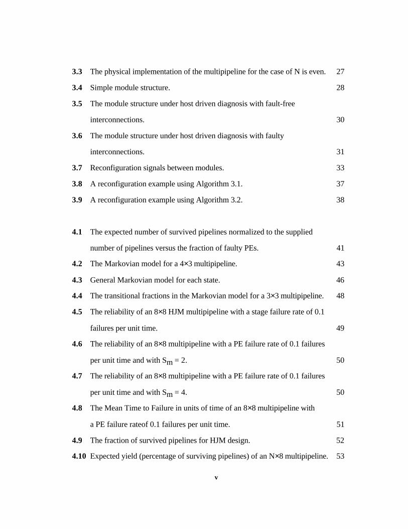
As shown in Figure 3.1, multiplexers are placed between stages to take inputs from

two previous stages and delivers one of them to the next stage. It is clear from Figure 3.1

that all the interconnects are of equal length except for the wraparound ones. By

reordering the PEs, we can make all the interconnections into equal lengths as we will see

in the next section.

3.2 Implementation

The goal of implementing the multipipeline is to get rid of the long wraparound wires

by making them equal to the other interconnects. Let ƒ be a function mapping each logical

PE in the logical architecture to its corresponding physical implementation and let (a,b) be

the indices of a PE in the logical architecture and (x,y) be the indices in the physical

implementation. The coordinates a and x are the vertical indices running from 0 to N-1.

On the other hand, b and y are the horizontal indices running from 0 to M-1. Hence, we

have ( , ) ( , )a bf

x y → . The logical architecture of Figure 3.1 is mapped to the physical

implementation shown in Figure 3.2. It is easy to verify that all the transformed

interconnects are of equal length. The mapping function and its proof are described below.

MUX

MUX

MUX

MUX

MUX

MUX

MUX

MUX

MUX

0,0

1,0

2,0 0,1

1,1

2,1

1,2

0,2

2,2 0,3

1,3

2,3

Figure 3.2 The physical architecture for the multipipeline.

25

Theorem 3.1:

The transformation defined below guarantees a constant length of interconnect.

2a If b is even, N is even, a ≤ (N-2)/2, 2a If b is even, N is odd, a ≤ (N-1)/2, 2N-1-2a If b is even, N is even, a > (N-2)/2, 2N-1-2a If b is even, N is odd, a > (N-1)/2,

x = 2a+1 If b is odd, N is even, a ≤ (N-2)/2, 2a+1 If b is odd, N is odd, a ≤ (N-3)/2, 2N-1-(2a+1) If b is odd, N is even, a > (N-2)/2, 2N-1-(2a+1) If b is odd, N is odd, a > (N-3)/2.

y = b.

Proof:

We prove the first case and all the others can be proved in a similar way. Consider the

case when b is even, N is even, and a ≤ (N-2)/2. The PE X(a,b) in the logical architecture

receives input from PEs A(a,b-1) and B[(a-1) mod N,b-1]. On the other hand, it sends

output to PEs C(a,b+1) and D[(a-1) mod N,b+1]. Using the above transformation, X will

be mapped to X'(2a,b). b is even ⇔ b-1 and b+1 are odd ⇒A(a,b-1) will be transformed

to A'(2a+1,b-1) and C(a,b+1) will be transformed to C'(2a+1,b+1). Two cases are going

to be considered:

case 1: a ≠ 0.

0<a < N ⇒ a mod N = a. (3.1)

0<a-1 < a < N⇒ (a-1) mod N = a-1. (3.2)

a-1 < a and a ≤ (N-2)/2 ⇒ (a-1) < (N-2)/2. (3.3)

26

Using (3.3) in the transformation above, B[(a-1) mod N,b-1]=B(a-1,b-1) is mapped to

B'[2(a-1)+1,b-1]=B'(2a-1,b-1) and D[(a-1) mod N,b+1]=D(a-1,b+1) is mapped to D'[2(a-

1)+1,b+1]=D'(2a-1,b+1).

In Figure 3.3 below, we see the physical implementation of a 4×4 multipipeline. Each

PE has a physical index in the upper side and a logical index in the lower side. It is clear

from this Figure that X' gets inputs from A' and B' and send outputs to C' and D' (take

X'(2,2) as an example).

MUX

MUX

MUX

MUX

MUX

MUX

MUX

MUX

MUX

0,0

1,0

3,0 0,1

2,1

3,1

1,2

0,2

3,2 0,3

2,3

3,3

MUX

MUX

MUX2,0

1,12,2 1,3

0,0

0,1

0,2

0,3

1,0 1,1 1,2 1,3

2,0 2,1 2,2 2,3

3,0 3,1 3,2 3,3

Figure 3.3 The physical implementation of the multipipeline for the case of N is even.

case 2: a = 0.

a=0 ⇒ (a-1) mod N = N-1. (3.4)

2N > N ⇒ 2N-2 > N-2 ⇒ 2(N-1) > N-2 ⇒ N-1 > (N-2)/2. (3.5)

Using (3.5) in the transformation, B[(a-1) mod N,b-1]=B[N-1,b-1] will be mapped to

B'[2N-1-(2(N-1)+1),b-1]=B'(0,b-1) and D[(a-1) mod N,b+1]=D[N-1,b+1] will be mapped

to D'[2N-1-(2(N-1)+1),b+1]=D'(0,b+1). It is also clear from Figure 3.3 that X' gets inputs

from A' and B' and sends outputs to C' and D' (take X'(0,2) as an example).

Q.E.D.

27

3.3 Diagnosis

Fault diagnosis is the detection and location of faulty elements so reconfiguration can

be performed over the array. The diagnosis algorithm should end by knowing the status --

faulty or healthy -- of all PEs in the multipipelines. Diagnosis in multipipelines depends on

the fault model assumed. In all the fault models, the reconfiguration control is assumed

fault-free due to its simplicity. Diagnosis in multipipelines could be distributed or host

driven. Each of these will be described in the next sections.

3.3.1 Distributed Diagnosis

To perform a distributed diagnosis, the status of the PE must be determined by a self

testing circuit. The modified structure of a module, which includes the PE of a non-fault-

tolerant multipipeline, is shown in Figure 3.4. The multiplexer, self testing circuit, status

flip flop F, and interconnections are assumed to be fault free. With this fault model, a

distributed runtime auto-reconfiguration can be implemented easily. The reconfiguration

algorithm is implemented with hardware in the control circuitry.

MUX

FSelfTestingCircuit

PE

Control

Figure 3.4 Simple module structure.

28

The control circuit obtains the status of the neighboring PEs by using some control

signals (to be described later in section 3.4.1) and the status of its PE. Based on this

information and the reconfiguration algorithm, the control circuit decides what is its input

and sets the multiplexer to get the required input and informs the four neighbors with its

decision. The reconfiguration algorithm is described later in section 3.4.

3.3.2 Host Driven Diagnosis

In most of the cases the multipipeline is driven by a host, hence error diagnosis can be

assigned to the host. With the help of the host, faults in interconnections can be detected.

So, diagnosis can be performed according to whether or not the assumption of fault-free

interconnections is retained.

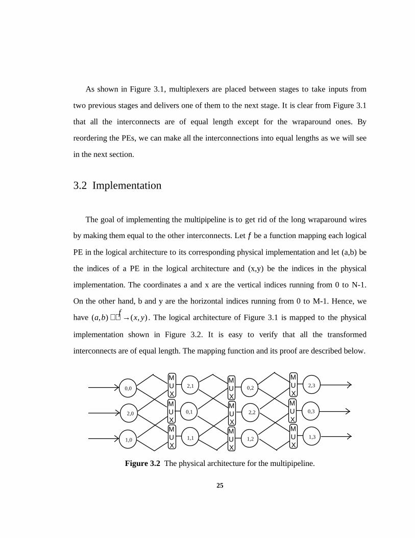
3.3.2.1 Fault-Free Interconnections

With the interconnections being fault free, the module structure of Figure 3.4 is

modified to handle the host control of the status flip-flops. This can be done by connecting

all the status flip flops of a column of PEs in a scan path format. The modified structure is

shown in Figure 3.5.

The host will perform the following sequence of operations: apply test vectors to the

multipipeline, read the multipipeline response, decide on the status of the PEs, set the

status flip flops of the PEs according to the diagnosis results, and finally activate the

execution of the reconfiguration algorithm.

29

MUX

F

PE

Control

Figure 3.5 The module structure under host driven diagnosis with fault-free

interconnections.

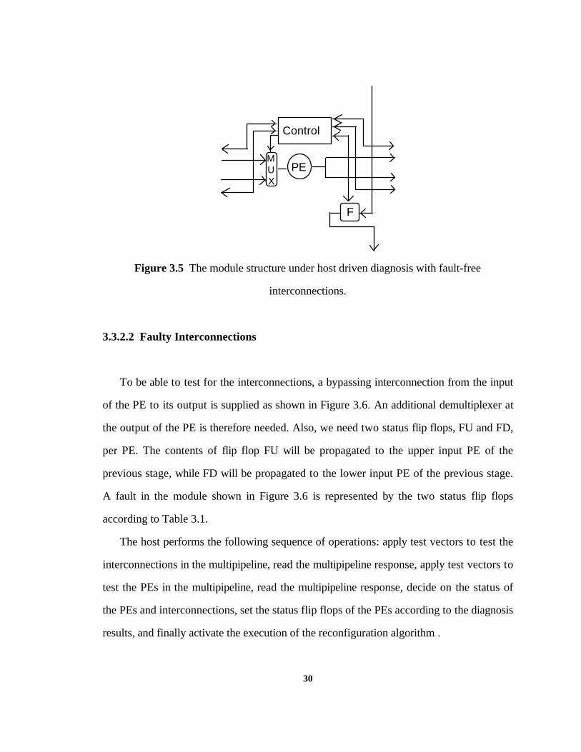
3.3.2.2 Faulty Interconnections

To be able to test for the interconnections, a bypassing interconnection from the input

of the PE to its output is supplied as shown in Figure 3.6. An additional demultiplexer at

the output of the PE is therefore needed. Also, we need two status flip flops, FU and FD,

per PE. The contents of flip flop FU will be propagated to the upper input PE of the

previous stage, while FD will be propagated to the lower input PE of the previous stage.

A fault in the module shown in Figure 3.6 is represented by the two status flip flops

according to Table 3.1.

The host performs the following sequence of operations: apply test vectors to test the

interconnections in the multipipeline, read the multipipeline response, apply test vectors to

test the PEs in the multipipeline, read the multipipeline response, decide on the status of

the PEs and interconnections, set the status flip flops of the PEs according to the diagnosis

results, and finally activate the execution of the reconfiguration algorithm .

30

MUX

FD

PE

Control

FU

MUX

DE

a

b

c d

e

fg

Figure 3.6 The module structure under host driven diagnosis with faulty interconnections.

Table 3.1 Values of FU and FD for different faults.

Type of Fault Status of FU Status of FD

No fault Good Good

PE is faulty Bad Bad

MUX is faulty Bad Bad

DEMUX is faulty Bad Bad

Line a is faulty Bad Good

Line b is faulty Good Bad

Line c is faulty Bad Bad

Line d is faulty Bad Bad

Line e is faulty Good Good

Line f is faulty Bad Bad

Line g is faulty Bad Bad

31

The diagnosis of the multipipeline ends by setting the status flip flops according to the

testing results. After that, a reconfiguration of the multipipeline is performed. The

reconfiguration of the multipipeline is discussed in the next section.

3.4 Reconfiguration

After locating the faults in the array, a reconfiguration of the array is performed. If the

error diagnosis is distributed, the self-testing circuits concurrently test the PEs and set the

status flip-flops according to the test results. If a fault is detected, an auto-reconfiguration

is initiated. On the other hand, if the error diagnosis is host driven, then the host performs

the testing in the simplest form of a periodic basis in a semi-concurrent way. If a fault is

detected, the host initiates the reconfiguration. The reconfiguration algorithm is

implemented with hardware in the control part of a module. The reconfiguration control of

a module communicates with the four neighboring PEs by using some control signals

which are described in the next section.

3.4.1 Control

Each module of the multipipeline communicates with its nearest two neighbors from

the previous stage and its nearest two neighbors of the following stage. The

communication between any two modules is done by using two control signals. The

control signals between the modules are shown in Figure 3.7.

The module X receives two input request signals from modules A and B. It can

acknowledge one of these requests only since a module can only be in one pipeline at a

time. On the other hand, module X receives the status of modules C and D by using

32

acknowledge signals. Based on the reconfiguration algorithm and the its status, module X

will request from either C or D to be the next stage of the pipeline passing through X by

using the request signals. The I/O control signals to the module are:

I_REQ_U

I_REQ_D

I_ACK_U

I_ACK_D

O_REQ_U

O_REQ_D

O_ACK_U

O_ACK_D

X

A

B

C

D

Stage iStage i-1 Stage i+1

Figure 3.7 Reconfiguration signals between modules.

I_REQ_U (I_REQ_D) : This signal is the input request signal to the module

from the upper (down) module in the previous stage. If this signal is asserted,

then the module is requested to be engaged in a pipeline passing through the

upper (down) module in the previous stage.

O_REQ_U (O_REQ_D) : This signal is the output request signal from the

module to the upper (down) module in the next stage. If this signal is asserted,

then the PE requests from the upper (down) module in the next stage to be

engaged in a pipeline passing through the module.

I_ACK_U (I_ACK_D) : This signal is the input acknowledgement request

signal to the module from the upper (down) module in the next stage. If this

signal is negated, then the upper (down) module in the next stage accepts the

request from the module, else it is rejected.

33

O_ACK_U(O_ACK_D) : This signal is the output acknowledgement signal

from the module to the upper (down) module in the previous stage. If this

signal is negated, then the module accepts the request from the upper (down)

module in the previous stage, else the request is rejected.

Each stage i in pipeline r will determine what is the previous stage i-1 in the pipeline

and what is the next stage i+1 in the pipeline by using the reconfiguration algorithm. The

reconfiguration algorithm will be discussed in the next section.

3.4.2 Algorithm

The reconfiguration algorithm is executed by all modules in parallel. For the case of

distributed diagnosis with one status flip flop, the algorithm can be summarized as follows.

If the module X in stage i is faulty then the module does not acknowledge any

of the requests from modules A and B in stage i-1. Similarly if both

acknowledgement signals from the two nearest modules C and D of the next stage

i+1 are high, there will be no acknowledgment. On the other hand if the module X

in stage i is healthy and at least one of the acknowledgement signals from modules

C and D in stage i+1 is low, a pipeline passing through the module X in stage i can

be formed. The module acknowledges one request, if it exists, to module A or B in

stage i-1 with a higher priority assigned to the upper module A. The module also

request from one of the two modules C and D in stage i+1 to be engaged in the

pipeline with priority to the upper module C.

The algorithm can be described in a simple Pascal code as follows:

34

ALGORITHM 3.1

IF (F=1) OR ( (I_ACK_U=1) AND (I_ACK_D=1)) THEN

BEGIN

O_ACK_U:=1;O_ACK_D:=1;

END

ELSEBEGIN

IF I_REQ_U=1 THEN

BEGIN

O_ACK_D:=1;O_ACK_U:=0;

END;IF I_REQ_U=0 THEN

O_ACK_D:=0;IF (I_REQ_U=1) OR (I_REQ_D=1) THEN

BEGIN

IF I_ACK_U=0 THEN

BEGIN

O_REQ_U:=1;O_REQ_D:=0;

END

ELSE IF I_ACK_D=0 THEN

BEGIN

O_REQ_U:=0;O_REQ_D:=1;

END;END;

END;

On the other hand if we have two status flip flops representing the state, the

reconfiguration algorithm is modified slightly. If the flip flop FU is set, then module X in

stage i cannot acknowledge the request from the upper module A in stage i-1. If the flip

flop FD is set, then module X cannot acknowledge the request from the lower module B

in stage i-1. The algorithm can be described in a simple Pascal code as follows:

35

ALGORITHM 3.2

IF (FU=1) THEN

O_ACK_U:=1IF (FD=1) THEN

O_ACK_D:=1IF ((FU=1) AND (FD=1)) OR ((I_ACK_U=1) AND (I_ACK_D=1)) THEN

BEGIN

O_ACK_U:=1O_ACK_D:=1

END

ELSEBEGIN

IF (I_REQ_U=1) AND (FU=0) THEN

BEGIN

O_ACK_D:=1;O_ACK_U:=0;

END;IF (I_REQ_U=0) AND (FD=0) THEN

O_ACK_D:=0;IF ((I_REQ_U=1) AND (FU=0)) OR

((I_REQ_D=1) AND (FD=0))THEN

BEGIN

IF I_ACK_U=0 THEN

BEGIN

O_REQ_U:=1;O_REQ_D:=0;

END

ELSE IF I_ACK_D=0 THEN

BEGIN

O_REQ_U:=0;O_REQ_D:=1;

END;END;

END;

We conjecture that the reconfiguration algorithms are optimal in the sense of finding

the maximum number of recovered pipelines in the presence of faults for the new

36

architecture presented in this chapter. This conjecture is based on running the algorithms

and examining their outputs many times. The algorithms are very simple to be

implemented in simple combinational logic circuits.

3.5 Examples

An example on using Algorithm 3.1 to reconfigure multipipelines with the assumption

that faults are only in the PEs is shown in Figure 3.8. The PEs marked X are faulty. The

bold lines are the active ones after the reconfiguration. It is clear that Algorithm 3.1 finds

the best solution.

MUX

MUX

MUX

MUX

MUX

MUX

MUX

MUX

MUX

0,0

1,0

0,1

1,1

1,2

0,2

0,3

1,3

X

X

X

Figure 3.8 A reconfiguration example using Algorithm 3.1.

A similar result using Algorithm 3.2 with faults occurring in both the interconnects and

the PEs is shown in Figure 3.9. The PE marked with X is faulty and the dotted

interconnections are also faulty. It is clear that Algorithm 3.2 finds the best solution.

37

MUX

MUX

MUX

MUX

MUX

MUX

MUX

MUX

MUX

0,0

1,0

0,1

1,1

1,2

0,2

0,3

1,3

X

Figure 3.9 A reconfiguration example using Algorithm 3.2.

After describing the new design, an evaluation of this design is needed. The

comparison between the new design and the design presented in Chapter 2 is the topic of

the next chapter.

38

Chapter 4

Simulation and Comparison

The following figures of merit [10] are suggested for evaluating a reconfiguration

scheme: Simplicity, efficiency, area, and locality. Simplicity refers to the execution time

of the reconfiguration algorithm. A simple algorithm requires a short execution time.

Efficiency refers to spare use. An efficient scheme wastes none or very few spare cells

and, thus, achieves a very high array survivability and harvest. Area refers to the overhead

of the added interconnect and reconfiguration circuitry. Low-overhead schemes are

desirable because a large silicon area increases the probability of having more defective

elements. Locality means that physical interconnections between logically adjacent cells in

a reconfigured array should have minimal lengths. It determines the maximum delay in

signal propagation, therefore limiting the clock rate at which the array can operate.

These figures of merit as well as reliability are used in this chapter to compare the new

design to the design presented in Chapter 2. The following labels are used:

1- HJM: The design presented in this thesis.

2- GUPTA: The design presented in [2] and reviewed in Section 2.3.

3- MIN: The straight-through pipeline design which is a non fault-tolerant

design. MIN represents the lower bound of simplicity, area, efficiency,

and reliability.

4- MAX: The design where the interconnection network between stages is

complete, i.e., every PE in stage i is connected to every PE in stage

39

i+1 . This design represents the upper bound of area and efficiency. It

represents also the upper bound of reliability if the interconnections

are assumed fault free.

4.1 Simplicity

Both algorithms presented (HJM and GUPTA) have fast execution times because they

are implemented in hardware, but the HJM algorithm is simpler. This is based on the fact

that HJM's algorithm is a parallel distributed algorithm where each PE performs the

reconfiguration in parallel without any sequence of reconfiguration. While GUPTA's

algorithm needs a sequence of reconfiguration phases as shown in Chapter 2: The top row

of PEs is first reconfigured, followed by the reconfiguration of the second row of PEs,

which is in turn followed by the third row, and so on. According to Chapter 3, the

execution of HJM's algorithm is done in parallel. So, HJM's algorithm does not need

sequencing control logic -- circuits to activate reconfiguration phases -- while GUPTA's

algorithm needs such logic.

4.2 Efficiency

To compare the efficiency of HJM's design to GUPTA's design, a simulation is

conducted on an 8x8 multipipeline. Faults are assumed to be randomly distributed within

the multipipeline with the interconnections assumed to be fault-free. The expected number

of recovered pipelines, normalized to the total number of pipelines supplied, is plotted as a

function of F (fraction of faulty PEs) as shown in Figure 4.1. From this figure, we can

conclude that GUPTA's design has a better performance than that of HJM's design if F is

40

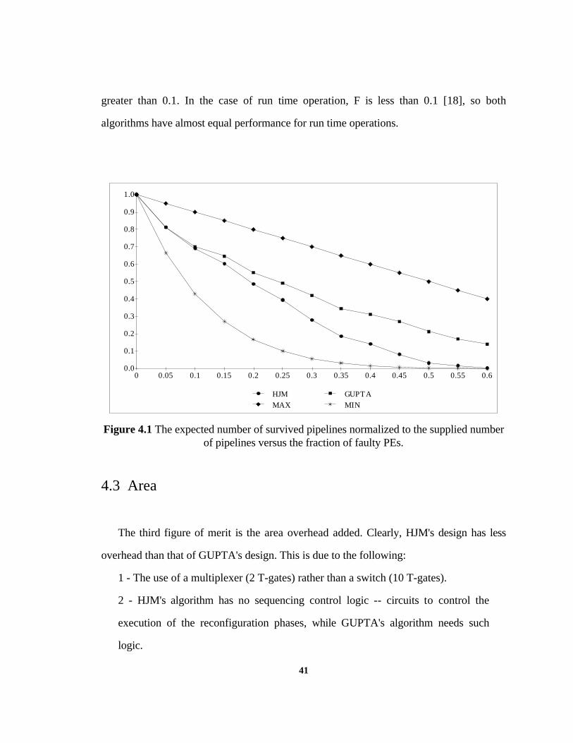
greater than 0.1. In the case of run time operation, F is less than 0.1 [18], so both

algorithms have almost equal performance for run time operations.

0.0

0.1

0.2

0.3

0.4

0.5

0.6

0.7

0.8

0.9

1.0

0 0.05 0.1 0.15 0.2 0.25 0.3 0.35 0.4 0.45 0.5 0.55 0.6

HJM GUPTA

MAX MIN

Figure 4.1 The expected number of survived pipelines normalized to the supplied numberof pipelines versus the fraction of faulty PEs.

4.3 Area

The third figure of merit is the area overhead added. Clearly, HJM's design has less

overhead than that of GUPTA's design. This is due to the following:

1 - The use of a multiplexer (2 T-gates) rather than a switch (10 T-gates).

2 - HJM's algorithm has no sequencing control logic -- circuits to control the

execution of the reconfiguration phases, while GUPTA's algorithm needs such

logic.

41

4.4 Locality

The largest advantage of HJM's design over GUPTA's design is in the locality

characteristic. In HJM the distance between any consecutive stages is always constant; in

GUPTA's design the length is dependent on fault distribution. This locality characteristic is

forced by the physical architecture, independent of the reconfiguration algorithm.

4.5 Reliability Evaluation

In this section, the reliability of HJM design is compared to that of GUPTA's design.

The reliability is calculated using Markov models for an 8×8 multipipeline. The PEs are

assumed to fail independently with a constant failure rate λ measured in failures per PE

per unit time. A system failure has occurred when the number of working pipelines

becomes less than a certain number Sm. Thus the reliability is defined as follows:

R(t) = Prob { S(t) ≥ Sm },

where S(t) is the number of survived pipelines at time t, and Sm is the minimum number of

survived pipelines that is needed for the multipipeline to be considered in a non-fatal

failure condition.

Before calculating the reliability of the multipipelines, the Markov model of the

multipipelines needs to be described.

42

4.5.1 Markovian Modeling

The Markov model for reliability prediction requires two assumptions [6,18] : PEs fail

independently in different moments, and the transition rate between two different error

states of a system of PEs (multipipeline) is constant.

To develop the model of the multipipeline, consider first the simple case of a 4×3

multipipeline. The Markov model for the multipipeline with Sm=2 is shown in Figure 4.2.

Each circle in that figure represents an ensemble of states. Each ensemble is represented

by (α,β), where α represents the number of survived pipelines and β represents the

number of faulty PEs. Initially, the multipipeline is in ensemble (4,0) and finally, the

multipipeline is in an ensemble (1,γ)≡(F), where γ is any number such that γ >2. There are

many states of the multipipeline that have 3 survived pipelines with 1 faulty PE. In fact,

the ensemble (3,1) has M×N states. On the other hand the ensemble (4,0) has only one

state.

4,0

3,1 3,33,2

2,2 2,3 2,4 2,5 2,6

F F F F F

Survived Pipelines = 4

Survived Pipelines = 3

Survived Pipelines = 2

Survived Pipelines < 2

Figure 4.2 The Markovian model for a 4×3 multipipeline.

43

The first fault in the multipipeline leads to losing one pipeline as shown in Figure 4.2.

The second fault in the multipipeline could lead to losing another pipeline if the first and

second faults occurred in PEs of the same column. Otherwise, the second fault will not

lead to losing a pipeline. In general, after the first fault, a fault may or may not lead to

losing a pipeline.

Consider the most general case of M×N multipipeline where a fatal failure is reached

when the number of survived pipelines is less than Sm. By inspection, the ensembles in the

Markov model are as follows:

one fault-free ensemble which has a single state.

1*(M-1)+1 ensembles each has N-1 fault-free pipelines.

2*(M-1)+1 ensembles each has N-2 fault-free pipelines.

...

k*(M-1)+1 ensembles each has N-k fault-free pipelines.

....

(N-Sm)*(M-1)+1 ensembles each has Sm fault-free pipelines.

(N-Sm)*(M-1)+1 fatal failure ensembles.

Hence, the total number of ensembles of the Markovian model is :

ST = 1 + 1*(M-1) + 1 + 2*(M-1) + 1 + 3*(M-1) + 1+. . .+ k*(M-1) + 1 +. . .+ (N-

Sm)*(M-1) + 1+ (N-Sm)*(M-1) +1

= (M-1)*{1+2+...+(N-Sm)}+(N-Sm)+1+(N-Sm)*(M-1)+1

= (M-1)*(N-Sm)*(N-Sm+1)/2 + (N-Sm)+(N-Sm)*(M-1)+2

= (N-Sm)*{(M-1)*(N-S m+1)/2 + M} + 2

44

If M=N, then ST will be O(N3). This shows the rapid growth of complexity of the

Markovian modeling. Initially in the Makov model, the multipipeline is in ensemble (N,0)

and finally, the multipipeline is in an ensemble (Sm-1,γ)≡(F), where γ is any number such

that γ >(N-Sm). In general, each ensemble of the Markov model can be represented as

shown in Figure 4.3.

From each ensemble (p,f) of the Markov model, there exists q transitions (PE failures)

to other ensembles of which r lead to a loss of a pipeline. Since the probabilities of failure

of the PEs are constant, equal, and independent, then the rate of pipeline failures from

ensemble (p,f) is the number of live PEs (N×M-f) times the PE failure rate (λ) times the

transitional fraction r/q (Fv). The transitional fractions Fv', Fh', Fv, and Fh are important

parameters that become increasingly burdensome to obtain analytically as N increases. For

small number of PEs, enumerating the states and grouping them into ensembles leads to

finding the actual values of the transitional fractions. For medium and large number of

PEs, the enumeration technique is not practical. Hence, for medium and large numbers of

PEs, simulation is used to determine the transitional fractions. The transitional fraction Fv'

is the fraction of PE failures which lead to loss of a pipeline while the multipipeline is in

the ensemble (p+1,f-1). Similarly, Fv is the fraction of PE failures which lead to loss of a

pipeline while the multipipeline is in the ensemble (p,f). On the other hand, Fh' is the

fraction of PE failures which do not lead to loss of a pipeline while the multipipeline is in

the ensemble (p,f-1). Similarly, Fh is the fraction of PE failures which do not lead to loss

of a pipeline while the multipipeline is in the ensemble (p,f). Let P(a,b)(t) be the probability

of being in ensemble (a,b). Then the following equation relates the ensembles in Figure

4.3.

dP (t)

dt(p,f)

= -λ (NxM-f) P (t)(p,f) + λ (NxM-f+1)[Fv' P (t)(p+1,f-1) (p,f-1)+ Fh' P (t)]

45

Ensemble (p,f) should be provided by Fh' and Fv' in order to determine the probability

of being in ensemble (p,f) at time t+∆t. Note that this probability is independent of Fv and

Fh because Fv+Fh=1.

p+1 , f-1

p , f-1

p-1 , f-1

p , f p , f+1

(NxM-f)Fvλ

(NxM-f)Fhλ

(NxM-f+1)Fv'λ

(NxM-f+1)Fh'λ

Figure 4.3 General Markovian model for each ensemble.

To get the transitional fractions Fv' and Fh' for each state, a simulation is performed.

For each ensemble, two variables Nv and Nh are defined. In ensemble (p,f), Nv(p,f) is the

number of times the ensemble is visited from ensemble (p+1,f-1) and Nh(p,f) is the number

of times the ensemble is visited from ensemble (p,f-1). Each time the ensemble is visited

either Nv(p,f) or Nh(p,f) is incremented. The procedure of getting Fh' and Fv' is then

written as follows:

Repeat 1000 times

Initialize the multipipeline to fault-free state.

repeat

Generate a fault

Move to the corresponding ensemble.

46

Increment either Nv or Nh

Until fatal-failure

Until done

for all ensembles do

Fv' = Nv(p,f) / [(Nv(p+1,f-1)+Nh(p+1,f-1)]

Fh' = Nh(p,f) / [(Nv(p,f-1)+Nh(p,f-1)]

endfor

The code written for getting the parameters Fv' and Fh' is listed in Appendix A.

To verify that the values of Fv' and Fh' determined using the above procedure

converge to their respective exact values, the transitional fractions are derived

theoretically for the case of 3×3 multipipeline with Sm=1. The Markov model for the

multipipeline is shown in Figure 4.4. Since the sum of the transitional fractions going out

from an ensemble sums to 1, comparing the vertical transitional fractions calculated to that

determined by simulation is sufficient. Table 4.1 shows the exact values of the transitional

fractions, values determined by simulation, and percentage error by using values

determined by simulation instead of the exact values. The simulation is done using 1000

and 5000 iterations. It is clear that as the number of iterations increase, the simulation

values tend to their corresponding exact values.

From Table 4.1, we can see that the maximum percentage error is 1.06% with 5000

itaerations. Hence, using simulation to get the transitional fractions is sufficient for

determining the reliability of the multipipelines.

The derivation of the exact values of the transitional fractions for the 3×3 multipipeline

is given in Appendix B.

47

Table 4.1 Comparison between the transitional fractions determined by simulation andtheir corresponding exact values.Simulation Simulation Percentage error Percentage error

Transitional Exact values values by using values by using valuesFractions values using 1000 using 5000 determined from determined from

iterations iterations 1000 iterations 5000 iterations

FV1 1 1.0000 1.0000 0.0000 0.0000FV2 1/4 0.2492 0.2506 0.3200 -0.2240FV3 1/7 0.1388 0.1435 2.8400 -0.4780FV4 4/7 0.5692 0.5721 0.3900 -0.1140FV5 13/54 0.2323 0.2382 3.5062 1.0595FV6 1 1.0000 1.0000 0.0000 0.0000FV7 91/205 0.4383 0.4404 1.2621 0.8003FV8 13/19 0.6783 0.6784 0.8638 0.8492FV9 1 1.0000 1.0000 0.0000 0.0000

3,0

2,1 2,32,2

1,2 1,3 1,4 1,5 1,6

F F F F F

FV1

FV2

FV3

FV4

FV5

PV6

FV7 FV8 FV9

FH2 FH4

FH3 FH5 FH7 FH8

Figure 4.4 The transitional fractions in the Markovian model for a 3×3 multipipeline.

Based on the Markov model developed, the reliability of the multipipelines is

computed. The results are discussed in the next section.

48

4.5.2 Results

To access the reliability of HJM's design and that of GUPTA's, a simulation is

performed over an 8×8 multipipeline. The reliability is defined to be the probability of

being in a non-fatal failure state at time t. The results of this simulation are shown in

Figure 4.5, Figure 4.6 and Figure 4.7 respectively. In Figure 4.5, the reliability of the HJM

multipipeline is plotted for different values of Sm. It is clear (trivial) that as Sm decreases,

the reliability increases. From Figure 4.6 and 4.7, we can see that HJM design has a good

reliability compared to GUPTA's design especially when Sm is large (i.e., when we have

small amount of hardware redundancy). Also, we can see that both HJM and GUPTA are

far better than the straight-through multipipeline.

T ime

0

0.1

0.2

0.3

0.4

0.5

0.6

0.7

0.8

0.9

1

0 1 2 3 4 5 6 7 8 9 10 11 12

Sm=8

Sm=7

Sm=6

Sm=5

Sm=4

Sm=3

Sm=2

Sm=1

Figure 4.5 The reliability of an 8×8 HJM multipipeline with a PE failure rate of 0.1failures per unit time.

49

0.0

0.1

0.2

0.3

0.4

0.5

0.6

0.7

0.8

0.9

1.0

0 0.15 0.3 0.45 0.6 0.75 0.9 1.05 1.2 1.35 1.5 1.65 1.8 1.95 2.1 2.25 2.4 2.55 2.7 2.85 3

Reliability

Time

GUPTA HJM

MAX MIN

Figure 4.6 The reliability of an 8×8 multipipeline with a PE failure rate of 0.1 failures perunit time and with Sm = 6.

0.0

0.1

0.2

0.3

0.4

0.5

0.6

0.7

0.8

0.9

1.0

0 0.4 0.8 1.2 1.6 2 2.4 2.8 3.2 3.6 4 4.4 4.8 5.2 5.6 6 6.4 6.8

Reliability

Time

GUPTA HJM

MAX MIN

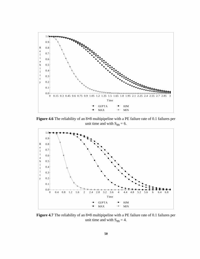
Figure 4.7 The reliability of an 8×8 multipipeline with a PE failure rate of 0.1 failures perunit time and with Sm = 4.

50

Another way for comparing the reliability is by comparing the mean time to failure

(MTTF). The results of simulation on the 8×8 multipipeline are shown in Figure 4.8.

According to that Figure, the MTTF of HJM's design approaches that of GUPTA's design

for large values of Sm. In fact, when Sm=7 we have MTTFHJM=MTTFGUPTA=MTTFMAX .

The code written for obtaining the reliability and the MTTF is listed in Appendix A.

0

2

4

6

8

10

12

14

8 7 6 5 4 3 2 1

MTTF

Sm as defined in section 4.5

GUPTA HJM

MAX MIN

Figure 4.8 The Mean Time to Failure in units of time of an 8×8 multipipeline with a PEfailure rate of 0.1 failures per unit time.

4.6 Effect of M and N

One of the questions that need to be addressed is what is the effect of increasing N or

M on the expected number of survived pipelines normalized to the total number of

pipelines? To get an answer for this question, simulations are carried by varying M, N, and

51

P - probability of failure of a PE. The results of the simulation are shown in Figure 4.9.

From this figure we can get the following conclusions:

1- as the probability of failure of a PE (P) increases for fixed N and M, the

number of survived pipelines decreases.

2- as M increases for fixed values of N and P, the number of survived pipelines

decreases.

3- as N increases for fixed values of M and P, the fraction of survived pipelines

tends to a constant limit after N becomes twice M.

The number of pipelines N

0

0.1

0.2

0.3

0.4

0.5

0.6

0.7

0.8

0.9

1 2 3 4 5 6 7 8 9 10 11 12 13 14 15 16 17 18 19 20

M=3 P=0.1 M=4 P=0.1 M=5 P=0.1

M=3 P=0.2 M=4 P=0.2 M=5 P=0.2

M=3 P=0.3 M=4 P=0.3 M=5 P=0.3

Figure 4.9 The fraction of survived pipelines for HJM design.

To emphasize on the fact that the yield - number of survived pipelines normalized to

the total number of pipelines - is relatively constant, the yield is plotted for M=8 and

different values of N and P as shown in Figure 4.10. According to that figure, we can

determine the number of pipelines needed for certain requirements. Assume that a

52

supercomputer (S) uses an 8×8 multipipeline. (S) will reach to a fatal failure if less than 8

pipelines are fault-free. Assume also that the probability of failure of a PE is 0.15. Thus we

need to find how many pipelines we should supply to have at least 8 of them working.

From Figure 4.10, we can see that for P=0.15, the yield is 60%. Hence, we need to supply

at least (8/0.6)≈13 pipelines to have 8 of them working. So, Figure 4.10 can be used as a

design aid for the fault-tolerant multipipelines.

T he probability of failure of a PE

0

10

20

30

40

50

60

70

80

90

100

0 0.05 0.1 0.15 0.2 0.25 0.3 0.35 0.4 0.45 0.5 0.55 0.6 0.65 0.7 0.75 0.8 0.85

N=4

N=6

N=8

N=10

N=12

N=14

N=16

N=18

N=20

Figure 4.10 Expected yield (percentage of surviving pipelines) of an N×8 multipipeline.

The code written to obtain Figure 4.9 and 4.10 is listed in Appendix A.

53

4.7 Summary

In this chapter, the multipipeline design presented in Chapter 3 is compared to the

design presented by [2]. Many figures of merit are used as the basis of comparison:

Simplicity, Efficiency, Area, Locality, and Reliability. In the reliability evaluation, Markov

models were developed and simulation is performed to get the results. The effect of M and

N is studied also in this chapter.

54

Chapter 5

Concluding Remarks

The thesis started with an introduction to multipipelines and their application. Then the

problem of fault-tolerant multipipelines is identified. In Chapter 2, the previous work on

fault-tolerant multipipelines is presented with emphasis on architecture, diagnosis, and

reconfiguration. In Chapter 3, the HJM design, which is the focus of this thesis, is

described with emphasis on implementation, diagnosis, and reconfiguration. In Chapter 4,

the new design is compared, using many figures of merit, to a well-known design

presented by [2]. In this last chapter, the accomplishments done in this thesis will be

summarized, and directions for future research will be given.

5.1 Accomplishments

A new design for fault-tolerant multipipelines has been given. The design is simpler

than other designs presented in the literature. It is characterized by its unity-length

interconnect that is independent of the fault distribution, less area overhead compared to

other designs, comparable efficiency for runtime operation, and good reliability and MTTF

especially when the hardware redundancy is small.

The accomplishments within this design, can be summarized as follows: A new

architecture for a multipipeline; a mapping algorithm from logical architecture to physical

implementation to get rid of the wraparound connects, forcing all interconnects to have a

55

unit-length; a diagnosis paradigm which gives the architecture of the PE depending on the

fault model assumed; a new reconfiguration algorithm for the fault-tolerant multipipeline

design when the interconnections are assumed fault-free, and another one when the

interconnections could be faulty; a Markov model for the general fault-tolerant

multipipeline problem; and finally a simulation procedure to get transitional fractions used

in the Markov model of multipipelines.

5.2 Future Research

The following are suggested as directions for further research.

Testing: As described in Chapter 3, self-testing of the PEs can lead to distributed

reconfiguration of multipipelines. A study is needed for finding the most suitable self-test

technique for multipipelines.

Architecture: Another interesting extension of the work in this thesis is have PEs

perform more than one function (for example, a PE can be reconfigured to be placed in

stage 2 or stage 5 in a pipeline). The questions that arise are:

a-How we should arrange the PEs in the physical structure.

b-How the PEs are interconnected.

c-What is the reconfiguration algorithm.

Failure Probability: A complete study of the probability of failure of PEs,

interconnections, and switches is needed. This will help in further evaluating the reliability

under faulty PEs, interconnections, and switches at the same time.

Mathematical Modeling: In Chapter 4, the effect of M and N on the survived number

of pipelines is studied. We can conclude that the curves in Figure 4.10, represents a single

curve. This could be an indication of the presence of an equation of that curve. In other

56

words, we can say that the number of survived pipelines is directly proportional to N. This

can also be verified from 4.9. An analytical study is needed to support the simulation

results.

Optimality: In Chapter 3, the conjecture that the reconfiguration algorithm is optimal

is given. A mathematical proof or disproof is needed for that conjecture.

57

Appendix A

The Turbo Pascal Code

In this appendix, the programs used in Chapter 4 are listed. The programs are written

in Turbo Pascal version 6.0 by BORLAND International. The programs require an IBM

PC or compatible to run. The programs that show examples need also a VGA display to

be executed.

A.1 Units Used

In this section, the units used by other programs are listed.

A.1.1 The Nodes Unit

UNIT NODES;

{THIS UNIT IS USED BY HJM DESIGN}

INTERFACE

{FAULTY=1 NONFAULTY=0} {REQUEST=1 NOREQUEST=0}

TYPE NODE=OBJECT { PE DESCRIPTION } X,Y:INTEGER; { POSITION OF PE } STATE:INTEGER; { STATE OF PE } PASS:BOOLEAN;

{ CONTROL SIGNALS } LREQ_U,LREQ_D:INTEGER; RREQ_U,RREQ_D:INTEGER; LACK_U,LACK_D:INTEGER; RACK_U,RACK_D:INTEGER;

{ METHODS OF OBJECT } PROCEDURE INIT; FUNCTION GET_LREQ_U:INTEGER; FUNCTION GET_LREQ_D:INTEGER; FUNCTION GET_RREQ_U:INTEGER; FUNCTION GET_RREQ_D:INTEGER; FUNCTION GET_LACK_U:INTEGER;

58

FUNCTION GET_LACK_D:INTEGER; FUNCTION GET_RACK_U:INTEGER; FUNCTION GET_RACK_D:INTEGER; PROCEDURE SET_LREQ_U(A:INTEGER); PROCEDURE SET_LREQ_D(A:INTEGER); PROCEDURE SET_RREQ_U(A:INTEGER); PROCEDURE SET_RREQ_D(A:INTEGER); PROCEDURE SET_LACK_U(A:INTEGER); PROCEDURE SET_LACK_D(A:INTEGER); PROCEDURE SET_RACK_U(A:INTEGER); PROCEDURE SET_RACK_D(A:INTEGER); PROCEDURE SETXY(A,B:INTEGER); PROCEDURE SETSTATE(S:INTEGER); FUNCTION GETSTATE:INTEGER; PROCEDURE UPDATE; FUNCTION GETCODE:INTEGER; FUNCTION NOCHANGE:BOOLEAN; END;

IMPLEMENTATION

PROCEDURE NODE.INIT; { INITIALIZE THE PE }BEGIN X:=0; Y:=0; STATE:=0; PASS:=FALSE; LREQ_U:=0; LREQ_D:=0; RREQ_U:=0; RREQ_D:=0; LACK_U:=0; LACK_D:=0; RACK_U:=0; RACK_D:=0;END;

{ GET FUNCTIONS }

FUNCTION NODE.GET_LREQ_U:INTEGER;BEGIN GET_LREQ_U:=LREQ_U;END;

FUNCTION NODE.GET_LREQ_D:INTEGER;BEGIN GET_LREQ_D:=LREQ_D;END;

FUNCTION NODE.GET_RREQ_U:INTEGER;BEGIN GET_RREQ_U:=RREQ_U;END;

FUNCTION NODE.GET_RREQ_D:INTEGER;BEGIN GET_RREQ_D:=RREQ_D;END;

FUNCTION NODE.GET_LACK_U:INTEGER;BEGIN GET_LACK_U:=LACK_U;END;

FUNCTION NODE.GET_LACK_D:INTEGER;BEGIN GET_LACK_D:=LACK_D;END;

59

FUNCTION NODE.GET_RACK_U:INTEGER;BEGIN GET_RACK_U:=RACK_U;END;

FUNCTION NODE.GET_RACK_D:INTEGER;BEGIN GET_RACK_D:=RACK_D;END;

{ SET PROCEDURES }

PROCEDURE NODE.SET_LREQ_U(A:INTEGER);BEGIN LREQ_U:=A;END;

PROCEDURE NODE.SET_LREQ_D(A:INTEGER);BEGIN LREQ_D:=A;END;

PROCEDURE NODE.SET_RREQ_U(A:INTEGER);BEGIN RREQ_U:=A;END;

PROCEDURE NODE.SET_RREQ_D(A:INTEGER);BEGIN RREQ_D:=A;END;

PROCEDURE NODE.SET_LACK_U(A:INTEGER);BEGIN LACK_U:=A;END;

PROCEDURE NODE.SET_LACK_D(A:INTEGER);BEGIN LACK_D:=A;END;

PROCEDURE NODE.SET_RACK_U(A:INTEGER);BEGIN RACK_U:=A;END;

PROCEDURE NODE.SET_RACK_D(A:INTEGER);BEGIN RACK_D:=A;END;

PROCEDURE NODE.SETXY(A,B:INTEGER);BEGIN X:=A; Y:=B;END;

{ UPDATE THE STATE OF THE PE }

PROCEDURE NODE.UPDATE;VAR P_LREQ_U,P_LREQ_D,P_LACK_U,P_LACK_D, P_RREQ_U,P_RREQ_D,P_RACK_U,P_RACK_D, P_STATE:INTEGER;BEGIN P_LREQ_U:=LREQ_U; P_LREQ_D:=LREQ_D; P_LACK_U:=LACK_U; P_LACK_D:=LACK_D; P_RREQ_U:=RREQ_U;

60

P_RREQ_D:=RREQ_D; P_RACK_U:=RACK_U; P_RACK_D:=RACK_D; P_STATE:=STATE;

IF (RACK_U=1) AND (RACK_D=1) THEN STATE:=1;

IF STATE=1 THEN BEGIN LACK_U:=1; LACK_D:=1; END ELSE BEGIN IF LREQ_U=1 THEN BEGIN LACK_D:=1; LACK_U:=0; END;

IF LREQ_U=0 THEN LACK_D:=0;

IF (LREQ_U=1) OR (LREQ_D=1) THEN BEGIN IF RACK_U=0 THEN BEGIN RREQ_U:=1; RREQ_D:=0; END ELSE IF RACK_D=0 THEN BEGIN RREQ_U:=0; RREQ_D:=1; END; END; END; IF (P_LREQ_U=LREQ_U) AND (P_LREQ_D=LREQ_D) AND (P_LACK_U=LACK_U) AND (P_LACK_D=LACK_D) AND (P_RREQ_U=RREQ_U) AND (P_RREQ_D=RREQ_D) AND (P_RACK_U=RACK_U) AND (P_RACK_D=RACK_D) AND (P_STATE=STATE) THEN PASS:=TRUE ELSE PASS:=FALSE;END;

{ RETURN THE CODE }{ CODE = 1 CONNECTED TO UPPER PE }{ CODE = 2 CONNECTED TO DOWN PE }{ CODE = 3 NOT CONNECTED }

FUNCTION NODE.GETCODE:INTEGER;BEGIN IF (RREQ_U=1) AND (RACK_U=0) THEN GETCODE:=0 ELSE IF (RREQ_D=1) AND (RACK_D=0) THEN GETCODE:=1 ELSE GETCODE:=2;END;

{ RETURN IF PE DOESNOT CHANGE STATE }

FUNCTION NODE.NOCHANGE;BEGIN NOCHANGE:=PASS;END;

61

{ SET STATE PROCEDURE }

PROCEDURE NODE.SETSTATE(S:INTEGER);BEGIN STATE:=S;END;

{ GET STATE FUNCTION }

FUNCTION NODE.GETSTATE:INTEGER;BEGIN GETSTATE:=STATE;END;END.

A.1.2 The Plot Unit

UNIT PLOT;{ THIS UNIT IS USED BY THE RELIABILITY PROGRAM }

INTERFACE

USES GRAPH,CRT;

CONST NMAX=10; MMAX=10;

TYPE MATRIX=ARRAY[0..NMAX*(MMAX-1)+1,0..NMAX+1] OF INTEGER; VECTOR=ARRAY[0..NMAX*(MMAX-1)+1,0..NMAX+1] OF REAL;

VAR DATAM:FILE OF MATRIX; DATAF:TEXT; CODE,RATESH,RATESV:MATRIX; RELIAB,NRELIAB:VECTOR; MTTF:ARRAY[1..NMAX] OF REAL; COLOR:ARRAY[1..NMAX] OF INTEGER; FACT:INTEGER; FREQUENCY:INTEGER;

PROCEDURE SETFACT(X:INTEGER); PROCEDURE INIT(M,N:INTEGER); PROCEDURE ITERATE(M,N:INTEGER;LEMBDA,DELTA,MAXTIME:REAL); PROCEDURE LOAD(FILNAME:STRING); PROCEDURE PRINT(N,X,Y:INTEGER);

IMPLEMENTATION

{ SET THE SCALE FACTOR }

PROCEDURE SETFACT(X:INTEGER);BEGIN FACT:=X;END;

{ INITIALIZE THE RELIABILITY }

PROCEDURE INIT(M,N:INTEGER);VAR I,J:INTEGER;BEGIN FOR I:=0 TO N*(M-1) DO FOR J:=0 TO N+1 DO BEGIN RELIAB[I,J]:=0; RATESH[I,J]:=0; RATESV[I,J]:=0; CODE[I,J]:=0; END;

62

RELIAB[1,1]:=1; NRELIAB:=RELIAB; FOR J:=1 TO N+1 DO FOR I:=1 TO 1+(M-1)*(J-1) DO CODE[I,J]:=1; CODE[N*(M-1),N+1]:=0;END;

{ PERFORM THE ITERATIONS TO GET THE RELIABILITY }

PROCEDURE ITERATE(M,N:INTEGER;LEMBDA,DELTA,MAXTIME:REAL);VAR TIME,TEMP,SUMP,SUMC:REAL; I,J,K:INTEGER; SCALE:REAL;BEGIN ASSIGN(DATAF,'C:\PROGRAM\TP\THESIS\PIPE8X8.DAT'); RESET(DATAF); APPEND(DATAF); SCALE:=FACT/DELTA; SETCOLOR(WHITE); LINE(5,450,5,50); LINE(5,450,635,450); TIME:=0; FOR I:=1 TO N DO MTTF[I]:=0; REPEAT

IF (ROUND(TIME/DELTA) MOD FREQUENCY)=0 THEN WRITE(DATAF,TIME:9:5,CHR(9)); FOR K:=1 TO N DO BEGIN SUMP:=0; SUMC:=0; FOR I:=1 TO N*(M-1)-1 DO FOR J:=1 TO K DO IF CODE[I,J]=1 THEN BEGIN SUMP:=SUMP+RELIAB[I,J]; SUMC:=SUMC+NRELIAB[I,J]; END; MTTF[K]:=MTTF[K]+SUMC*DELTA; SETCOLOR(COLOR[K]); IF (ROUND(TIME/DELTA) MOD FREQUENCY)=0 THEN WRITE(DATAF,SUMC:9:5,CHR(9)); LINE(5+ROUND((TIME-DELTA)*SCALE),450-ROUND(SUMP*350),5+ROUND(TIME*SCALE),450-ROUND(SUMC*350)); END; IF (ROUND(TIME/DELTA) MOD FREQUENCY)=0 THEN WRITELN(DATAF);

RELIAB:=NRELIAB;

FOR I:=1 TO N*(M-1)-1 DO FOR J:=1 TO N DO BEGIN TEMP:=-LEMBDA*(N*M-I-J+2)*RELIAB[I,J]; IF (CODE[I,J-1]=1) AND ((RATESH[I,J-1]+RATESV[I,J-1]) <>0) THEN TEMP:=LEMBDA*(N*M-I-J+2+1)*(RATESV[I,J]/(RATESV[I,J-1]+RATESH[I,J-1]))*RELIAB[I,J-1]+TEMP; IF (CODE[I-1,J]=1) AND ((RATESH[I-1,J]+RATESV[I-1,J]) <>0) THEN TEMP:=LEMBDA*(N*M-I-J+2+1)*(RATESH[I,J]/(RATESV[I-1,J]+RATESH[I-1,J]))*RELIAB[I-1,J]+TEMP; TEMP:=TEMP*DELTA; NRELIAB[I,J]:=TEMP+RELIAB[I,J]; END; J:=N+1; FOR I:=1 TO N*(M-1)-1 DO BEGIN IF (RATESH[I,J-1]+RATESV[I,J-1]) <> 0 THEN

63

TEMP:=LEMBDA*(N*M-I-J+2+1)*(RATESV[I,J]/(RATESV[I,J-1]+RATESH[I,J-1]))*RELIAB[I,J-1] ELSE TEMP:=0; TEMP:=TEMP*DELTA; NRELIAB[I,J]:=TEMP+RELIAB[I,J]; END;

TIME:=TIME+DELTA; UNTIL (TIME > MAXTIME); WRITELN(DATAF); FOR I:=1 TO N DO WRITELN(DATAF,I,CHR(9),MTTF[I]:9:5); WRITELN(DATAF); WRITELN(DATAF); CLOSE(DATAF);END;

{ LOAD THE TRANSITIONAL FRACTIONS }

PROCEDURE LOAD(FILNAME:STRING);BEGIN ASSIGN(DATAM,FILNAME); RESET(DATAM); READ(DATAM,RATESH,RATESV); CLOSE(DATAM);END;

{ PRINT A MESSAGE }

PROCEDURE PRINT(N,X,Y:INTEGER);VAR S1,S2:STRING; I:INTEGER;BEGIN S2:=''; FOR I:=1 TO N DO BEGIN STR(MTTF[I]:9:5,S1); S2:=S2+S1; END; OUTTEXTXY(X,Y,S2);END;

END.

A.2 The Transitional Fractions Programs

These programs determines the transitional fractions for the MAX, MIN, GUPTA, and

HJM Designs.

A.2.1 MAX's and MIN's transitional fractions

PROGRAM MAXMIN;{ THIS PROGRAM DERIVES THE TRANSITIONAL FRACTIONS FOR GUPTA DESIGN }{ FOR THE CASE OF 8X8 MULTIPIPELINE }

USES GRAPH,CRT;

CONST MMAX=10; NMAX=10;

TYPE NODE=RECORD

64

S:INTEGER; X,Y:INTEGER; END; MATRIX=ARRAY[0..NMAX*(MMAX-1)+1,0..NMAX+1] OF INTEGER; VECTOR=ARRAY[0..NMAX*(MMAX-1)+1,0..NMAX+1] OF REAL;

VAR M,N:INTEGER; XPA,PA:ARRAY[1..MMAX,1..NMAX] OF NODE; I,J:INTEGER; SP,COUNT,PROB:INTEGER; SURVIVE:INTEGER; DATAM:FILE OF MATRIX; CODE,RATESH,RATESV:MATRIX; RELIAB,NRELIAB:VECTOR; INDEXI,INDEXJ,SPLAST:INTEGER;

{ INITIALIZE THE TRANSITIONAL FRACTIONS }

PROCEDURE INIT;VAR I,J:INTEGER;BEGIN FOR I:=0 TO N*(M-1) DO FOR J:=0 TO N+1 DO BEGIN RELIAB[I,J]:=0; RATESH[I,J]:=0; RATESV[I,J]:=0; CODE[I,J]:=0; END; RELIAB[1,1]:=1; NRELIAB:=RELIAB; FOR J:=1 TO N+1 DO FOR I:=1 TO 1+(M-1)*(J-1) DO CODE[I,J]:=1; CODE[N*(M-1),N+1]:=0;END;

{ INJECT ONE FAULTY PE }

PROCEDURE INJECTONE;BEGIN PA:=XPA; REPEAT I:=RANDOM(M)+1; J:=RANDOM(N)+1; UNTIL (PA[I,J].S <> 1); PA[I,J].S:=1; XPA:=PA;END;

{ INITIALIZE THE MULTIPIPELINE }

PROCEDURE INITIALIZE;BEGIN FOR I:=1 TO M DO FOR J:=1 TO N DO BEGIN PA[I,J].S:=0; PA[I,J].X:=0; PA[I,J].Y:=0; END; XPA:=PA;END;

{ RUN THE SIMULATION ALGORITHM ON MAX DESIGN }

PROCEDURE RUNMAX;VAR I,J,K,L,Z:INTEGER; ENDIT:BOOLEAN;BEGIN

65

K:=0; FOR I:=1 TO M DO BEGIN Z:=0; FOR J:=1 TO N DO IF PA[I,J].S=1 THEN Z:=Z+1; IF Z > K THEN K:=Z; END; SURVIVE:=N-K;END;

{ RUN THE SIMULATION ALGORITHM ON MIN DESIGN }

PROCEDURE RUNMIN;VAR I,J,K,L,Z:INTEGER; ENDIT:BOOLEAN;BEGIN K:=N; FOR J:=1 TO N DO BEGIN Z:=0; FOR I:=1 TO M DO IF PA[I,J].S=1 THEN Z:=1; IF Z =1 THEN K:=K-1; END; SURVIVE:=K;END;

{ STORE THE TRANSITIONAL FRACTIONS }

PROCEDURE STORE(FILNAME:STRING);BEGIN ASSIGN(DATAM,FILNAME); REWRITE(DATAM); WRITE(DATAM,RATESH,RATESV); CLOSE(DATAM);END;

{ DERIVE THE TRANSITIONAL FRACTIONS FOR MAX DESIGN }

PROCEDURE DERIVE_MAX(STAT:INTEGER);BEGIN CLRSCR; FOR COUNT:=1 TO STAT DO BEGIN GOTOXY(10,10); WRITELN(COUNT); INITIALIZE; INDEXI:=0; INDEXJ:=1; SPLAST:=N; REPEAT RUNMAX; SP:=SURVIVE; IF SP = SPLAST THEN BEGIN INC(INDEXI); INC(RATESH[INDEXI,INDEXJ]); END; IF SP < SPLAST THEN BEGIN INC(INDEXJ); INC(RATESV[INDEXI,INDEXJ]); END; INJECTONE; SPLAST:=SP;

66

UNTIL SP=0; END;END;

{ DERIVE THE TRANSITIONAL FRACTIONS FOR THE MIN DESIGN }

PROCEDURE DERIVE_MIN(STAT:INTEGER);BEGIN CLRSCR; FOR COUNT:=1 TO STAT DO BEGIN GOTOXY(10,10); WRITELN(COUNT); INITIALIZE; INDEXI:=0; INDEXJ:=1; SPLAST:=N; REPEAT RUNMIN; SP:=SURVIVE; IF SP = SPLAST THEN BEGIN INC(INDEXI); INC(RATESH[INDEXI,INDEXJ]); END; IF SP < SPLAST THEN BEGIN INC(INDEXJ); INC(RATESV[INDEXI,INDEXJ]); END; INJECTONE; SPLAST:=SP; UNTIL SP=0; END;END;

BEGIN {--MAIN--} M:=8; N:=8; INIT; DERIVE_MAX(1000); STORE('C:\WINWORD\THESIS\PRGS\MAALG.RAT'); INIT; DERIVE_MIN(1000); STORE('C:\WINWORD\THESIS\PRGS\MIALG.RAT'); READLN;END.

A.2.2 GUPTA's transitional fractions

PROGRAM GUPTAPIPELINES;{ THIS PROGRAM DERIVES THE TRANSITIONAL FRACTIONS FOR GUPTA DESIGN }{ FOR THE CASE OF 8X8 MULTIPIPELINE }

USES GRAPH,CRT;

CONST MMAX=10; NMAX=10;

TYPE NODE=RECORD { PE DESCRIPTION } S:INTEGER; X,Y:INTEGER; END; MATRIX=ARRAY[0..NMAX*(MMAX-1)+1,0..NMAX+1] OF INTEGER; VECTOR=ARRAY[0..NMAX*(MMAX-1)+1,0..NMAX+1] OF REAL;

VAR M,N:INTEGER;

67

XPA,PA:ARRAY[1..MMAX,1..NMAX] OF NODE; I,J:INTEGER; SP,COUNT,PROB:INTEGER; SURVIVE:INTEGER; DATAF:TEXT; SUM:INTEGER; DATAM:FILE OF MATRIX; CODE,RATESH,RATESV:MATRIX; INDEXI,INDEXJ,SPLAST:INTEGER;

{ INITILAIZE TRANSITIONAL FRACTIONS }

PROCEDURE INIT;VAR I,J:INTEGER;BEGIN FOR I:=0 TO N*(M-1) DO FOR J:=0 TO N+1 DO BEGIN RATESH[I,J]:=0; RATESV[I,J]:=0; CODE[I,J]:=0; END; FOR J:=1 TO N+1 DO FOR I:=1 TO 1+(M-1)*(J-1) DO CODE[I,J]:=1; CODE[N*(M-1),N+1]:=0;END;

{ INJECT ONE FAULTY PE }

PROCEDURE INJECTONE;BEGIN PA:=XPA; REPEAT I:=RANDOM(M)+1; J:=RANDOM(N)+1; UNTIL (PA[I,J].S <> 1); PA[I,J].S:=1; XPA:=PA;END;

{ CONNECT THE PE'S }

PROCEDURE CONNECT;VAR XN,YN,XPN:INTEGER;BEGIN SURVIVE:=0; FOR J:=1 TO N DO BEGIN I:=1; XN:=PA[I,J].X; YN:=PA[I,J].Y; WHILE (XN>0) AND (YN>0) AND (XN<M) AND (YN <=N) DO BEGIN XPN:=XN; XN:=PA[XN,YN].X; YN:=PA[XPN,YN].Y; END; IF XN =M THEN BEGIN INC(SURVIVE); I:=1; XN:=PA[I,J].X; YN:=PA[I,J].Y;

WHILE (XN<M) DO BEGIN XPN:=XN; XN:=PA[XN,YN].X; YN:=PA[XPN,YN].Y;

68

END; END; END;END;

{ INITIALIZE THE MULTIPIPELINE }

PROCEDURE INITIALIZE;BEGIN FOR I:=1 TO M DO FOR J:=1 TO N DO BEGIN PA[I,J].S:=0; PA[I,J].X:=0; PA[I,J].Y:=0; END; XPA:=PA;END;

{ RUN THE SIMULATION ALGORITHM }

PROCEDURE RUN;VAR I,J,K,L,Z:INTEGER; ENDIT:BOOLEAN;BEGIN FOR J:=1 TO N DO BEGIN IF PA[1,J].S=0 THEN BEGIN PA[1,J].S:=2; K:=J; ENDIT:=FALSE; FOR I:=1 TO M-1 DO BEGIN IF NOT ENDIT THEN BEGIN L:=1; WHILE (PA[I+1,L].S <> 0) AND (L<N) DO INC(L); IF PA[I+1,L].S = 0 THEN BEGIN PA[I,K].X:=I+1; PA[I,K].Y:=L; PA[I+1,L].S:=2;

IF L>K THEN BEGIN FOR Z:=K+1 TO L-1 DO PA[I,Z].S:=3; END; IF L<K THEN BEGIN FOR Z:=L+1 TO K-1 DO PA[I+1,Z].S:=3; END; K:=L; END ELSE ENDIT:=TRUE; END END; END; END;END;

{ STORE THE TRANSITIONAL FRACTIONS }

PROCEDURE STORE(FILNAME:STRING);BEGIN ASSIGN(DATAM,FILNAME); REWRITE(DATAM);

69

WRITE(DATAM,RATESH,RATESV); CLOSE(DATAM);END;

{ DERIVE THE TRANSITIONAL FRACTIONS }

PROCEDURE DERIVE(STAT:INTEGER);BEGIN CLRSCR; FOR COUNT:=1 TO STAT DO BEGIN GOTOXY(10,10); WRITELN(COUNT); INITIALIZE; INDEXI:=0; INDEXJ:=1; SPLAST:=N; REPEAT RUN; CONNECT; SP:=SURVIVE; IF SP = SPLAST THEN BEGIN INC(INDEXI); INC(RATESH[INDEXI,INDEXJ]); END; IF SP < SPLAST THEN BEGIN INC(INDEXJ); INC(RATESV[INDEXI,INDEXJ]); END; INJECTONE; SPLAST:=SP; UNTIL SP=0; END;END;

BEGIN {--MAIN--} M:=8; N:=8; INIT; DERIVE(1000); STORE('C:\WINWORD\THESIS\PRGS\GUALG.RAT'); READLN;END.

A.2.3 HJM's transitional fractions

PROGRAM HJM_PIPELINES;{ THIS PROGRAM DERIVES THE TRANSITIONAL FRACTIONS FOR HJM DESIGN }{ FOR THE CASE OF 8X8 MULTIPIPELINE }

USES NODES,GRAPH,CRT;

CONST MMAX=10; NMAX=10;

TYPE MATRIX=ARRAY[0..NMAX*(MMAX-1)+1,0..NMAX+1] OF INTEGER; VECTOR=ARRAY[0..NMAX*(MMAX-1)+1,0..NMAX+1] OF REAL;

VAR M,N:INTEGER; XPA,PA:ARRAY[1..MMAX,1..NMAX] OF NODE; I,J:INTEGER; SP,COUNT,PROB:INTEGER; DATAM:FILE OF MATRIX; CODE,RATESH,RATESV:MATRIX; INDEXI,INDEXJ,SPLAST:INTEGER;

70

{ INITIALIZE THE TRANSITIONAL FRACTIONS }PROCEDURE INIT;VAR I,J:INTEGER;BEGIN FOR I:=0 TO N*(M-1) DO FOR J:=0 TO N+1 DO BEGIN RATESH[I,J]:=0; RATESV[I,J]:=0; CODE[I,J]:=0; END; FOR J:=1 TO N+1 DO FOR I:=1 TO 1+(M-1)*(J-1) DO CODE[I,J]:=1; CODE[N*(M-1),N+1]:=0;END;

{ INJECT ONE FAULTY PE IN THE MULTIPIPELINE }

PROCEDURE INJECTONE;BEGIN PA:=XPA; REPEAT I:=RANDOM(M)+1; J:=RANDOM(N)+1; UNTIL (PA[I,J].GETSTATE <> 1); PA[I,J].SETSTATE(1); XPA[I,J].SETSTATE(1);END;

{ INITIALIZE THE MULTIPIPELINE }

PROCEDURE INITIALIZE;BEGIN FOR I:=1 TO M DO FOR J:=1 TO N DO BEGIN PA[I,J].INIT; PA[I,J].SETXY(I,J); END; XPA:=PA;END;

{ GET CONTROL SIGNALS STATUS }

PROCEDURE GETVARS(I,J:INTEGER;VAR I1,I2,I3,I4:INTEGER);VAR K:INTEGER; TEMP:INTEGER;BEGIN IF I=1 THEN BEGIN I1:=1; I2:=0; I3:=PA[I+1,J].GET_LACK_D; I4:=PA[I+1,(J MOD N)+1].GET_LACK_U; END ELSE IF I=M THEN BEGIN IF ODD(I) THEN K:=1 ELSE K:=0; TEMP:=(J-1+K-1) MOD N; IF TEMP < 0 THEN TEMP:=TEMP+N; I1:=PA[I-1,TEMP+1].GET_RREQ_D; I2:=PA[I-1,((J+K-1)MOD N)+1].GET_RREQ_U; I3:=0; I4:=0; END ELSE BEGIN IF ODD(I) THEN K:=1 ELSE K:=0;

71

TEMP:=(J-1+K-1) MOD N; IF TEMP < 0 THEN TEMP:=TEMP +N; I1:=PA[I-1,TEMP+1].GET_RREQ_D; I2:=PA[I-1,((J+K-1) MOD N)+1].GET_RREQ_U; I3:=PA[I+1,TEMP+1].GET_LACK_D; I4:=PA[I+1,((J+K-1) MOD N)+1].GET_LACK_U; END;END;

{ SET CONTROL SIGNALS STATUS }

PROCEDURE SETVARS(I,J:INTEGER;O1,O2,O3,O4:INTEGER);VAR K:INTEGER; TEMP:INTEGER;BEGIN IF I=1 THEN BEGIN PA[I+1,J].SET_LREQ_D(O3); PA[I+1,(J MOD N)+1].SET_LREQ_U(O4); END ELSE IF I=M THEN BEGIN IF ODD(I) THEN K:=1 ELSE K:=0; TEMP:=(J-1+K-1) MOD N; IF TEMP<0 THEN TEMP:=TEMP+N; PA[I-1,TEMP+1].SET_RACK_D(O1); PA[I-1,((J+K-1)MOD N)+1].SET_RACK_U(O2); END ELSE BEGIN IF ODD(I) THEN K:=1 ELSE K:=0; TEMP:=(J-1+K-1) MOD N; IF TEMP<0 THEN TEMP:=TEMP+N; PA[I-1,TEMP+1].SET_RACK_D(O1); PA[I-1,((J+K-1) MOD N)+1].SET_RACK_U(O2); PA[I+1,TEMP+1].SET_LREQ_D(O3); PA[I+1,((J+K-1) MOD N)+1].SET_LREQ_U(O4); END;END;

{ RUN THE SIMULATION ALGORITHM }

PROCEDURE RUN;VAR EXIT:BOOLEAN; I1,I2,I3,I4:INTEGER; O1,O2,O3,O4:INTEGER;BEGIN REPEAT EXIT:=TRUE; FOR I:=1 TO M DO FOR J:=1 TO N DO BEGIN GETVARS(I,J,I1,I2,I3,I4); PA[I,J].SET_LREQ_U(I1); PA[I,J].SET_LREQ_D(I2); PA[I,J].SET_RACK_U(I3); PA[I,J].SET_RACK_D(I4); PA[I,J].UPDATE; O1:=PA[I,J].GET_LACK_U; O2:=PA[I,J].GET_LACK_D; O3:=PA[I,J].GET_RREQ_U; O4:=PA[I,J].GET_RREQ_D; SETVARS(I,J,O1,O2,O3,O4); EXIT:=EXIT AND PA[I,J].NOCHANGE; END; UNTIL EXIT;END;

{ DETERMINE THE NUMBER OF SURVIVED PIPELINES }

72

FUNCTION SURVIVE:INTEGER;VAR SUM:INTEGER;BEGIN I:=1; SUM:=0; FOR J:=1 TO N DO SUM:=SUM+(1-PA[I,J].GET_LACK_U); SURVIVE:=SUM;END;

{ STORE THE TRANSITIONAL FRACTIONS }

PROCEDURE STORE(FILNAME:STRING);BEGIN ASSIGN(DATAM,FILNAME); REWRITE(DATAM); WRITE(DATAM,RATESH,RATESV); CLOSE(DATAM);END;

{ DERIVE THE TRANSITIONAL FRACTIONS }

PROCEDURE DERIVE(STAT:INTEGER);BEGIN CLRSCR; FOR COUNT:=1 TO STAT DO BEGIN GOTOXY(10,10); WRITELN(COUNT); INITIALIZE; INDEXI:=0; INDEXJ:=1; SPLAST:=N; REPEAT RUN; SP:=SURVIVE; IF SP = SPLAST THEN BEGIN INC(INDEXI); INC(RATESH[INDEXI,INDEXJ]); END; IF SP < SPLAST THEN BEGIN INC(INDEXJ); INC(RATESV[INDEXI,INDEXJ]); END; INJECTONE; SPLAST:=SP; UNTIL SP=0; END;END;

BEGIN { -- MAIN -- } M:=8; N:=8; INIT; DERIVE(1000); STORE('C:\WINWORD\THESIS\PRGS\MYALG.RAT'); READLN;END.

A.3 Reliability and MTTF Calculations

This program calculates the reliabilities of the four designs and plot them on one graph.

73

PROGRAM RELIABILITY_PLOT;{ THIS PROGRAM PLOTS THE RELIABILITIES OF THE FOUR DESIGNS: }{ MAX , MIN , GUPTA , AND HJM }

USES GRAPH,CRT,PLOT;

CONST DELTA = 0.1 ; MAXTIME = 25 ; LEMBDA = 0.1 ;

VAR M,N:INTEGER; I,J:INTEGER; DATAM:FILE OF MATRIX;

{ INITIALIZE THE GRAPH UNIT }

PROCEDURE GRINIT;VAR GD,GM:INTEGER;BEGIN GD:=DETECT; INITGRAPH(GD,GM,'');END;

BEGIN GRINIT; M:=8; N:=8; SETFACT(2); FREQUENCY:=5;

{ RELIABILITY OF MAX DESIGN }

INIT(M,N); FOR I:=1 TO N DO COLOR[I]:=CYAN; LOAD('C:\PROGRAM\TP\THESIS\MAALG.RAT'); ITERATE(M,N,LEMBDA,DELTA,MAXTIME); PRINT(N,10,17);

{ RELIABILITY OF MIN DESIGN }

INIT(M,N); FOR I:=1 TO N DO COLOR[I]:=MAGENTA; LOAD('C:\PROGRAM\TP\THESIS\MIALG.RAT'); ITERATE(M,N,LEMBDA,DELTA,MAXTIME); PRINT(N,10,24);

{ RELIABILITY OF GUPTA DESIGN }

INIT(M,N); FOR I:=1 TO N DO COLOR[I]:=RED; LOAD('C:\PROGRAM\TP\THESIS\GUALG.RAT'); ITERATE(M,N,LEMBDA,DELTA,MAXTIME); PRINT(N,10,1);

{ RELIABILITY OF HJM DESIGN }

INIT(M,N); FOR I:=1 TO N DO COLOR[I]:=YELLOW; LOAD('C:\PROGRAM\TP\THESIS\MYALG.RAT'); ITERATE(M,N,LEMBDA,DELTA,MAXTIME); PRINT(N,10,9);

READLN;END.

74

A.4 Yield and reconfiguration examples

These programs calculates the yield and also display reconfiguration examples for GUPTAand HJM designs.

A.4.1 GUPTA's Design

PROGRAM GUPTAPIPELINES;{ THIS PROGRAM SHOWS EXAMPLES OF RECONFIGURATIONS AS WELL AS PERFORMING SIMULATIONS TO GET THE YIELD - EXPECTED NUMBER OF SURVIVED PIPELINES NORMALIZED TO THE TOTAL NUMBER OF PIPELINES }

USES GRAPH,CRT;

CONST MMAX=9; NMAX=20;

TYPE NODE=RECORD S:INTEGER; X,Y:INTEGER; END;

VAR M,N:INTEGER; PA:ARRAY[1..MMAX,1..NMAX] OF NODE; I,J,H:INTEGER; PSTR,XSTR:STRING; SP,COUNT,PROB:INTEGER; SURVIVE:INTEGER; DATAF:TEXT; SUM:INTEGER; MAVG:REAL; CHOICE:INTEGER;

{ DRAW A PE }

PROCEDURE BOX(A,B:INTEGER;COLOR:INTEGER);BEGIN SETFILLSTYLE(1,COLOR); BAR(40*A+10,40*B+10,40*A+25,40*B+25); SETCOLOR(RED); RECTANGLE(40*A+10,40*B+10,40*A+25,40*B+25);END;

[ DRAW ARROW }

PROCEDURE ARROW(X,Y:INTEGER);BEGIN LINE(X,Y,X-20,Y); LINE(X,Y,X-4,Y-4); LINE(X,Y,X-4,Y+4);END;

{ INITIALIZE THE GRAPH UNIT }

PROCEDURE GRINIT;VAR GD,GM:INTEGER;BEGIN GD:=DETECT; INITGRAPH(GD,GM,'');END;

{ DRAW THE MULTIPIPELINE }

75

PROCEDURE DRAW;VAR I,J:INTEGER;BEGIN SETCOLOR(MAGENTA); RECTANGLE(0,0,639,479); FOR I:=1 TO M DO FOR J:=1 TO N DO IF PA[I,J].S=0 THEN BOX(I,J,YELLOW) ELSE BOX(I,J,BLUE);END;

{ REDRAW THE MULTIPIPELINE AFTER CHANGES }

PROCEDURE REDRAW;VAR I,J:INTEGER;BEGIN SETCOLOR(MAGENTA); RECTANGLE(0,0,639,479); FOR I:=1 TO M DO FOR J:=1 TO N DO IF PA[I,J].S=0 THEN BOX(I,J,YELLOW) ELSE IF PA[I,J].S=1 THEN BOX(I,J,BLUE) ELSE IF PA[I,J].S=2 THEN BOX(I,J,YELLOW) ELSE IF PA[I,J].S=3 THEN BOX(I,J,RED);END;

{ DRAW AN INPUT LINE }

PROCEDURE INPUT(A:INTEGER);CONST ONCOLOR=RED;BEGIN SETCOLOR(ONCOLOR); LINE(40*1+10+7,40*A+10+7,40*1+10+7-30,40*A+10+7);END;

{ DRAW AN OUTPUT LINE }

PROCEDURE OUTPUT(A:INTEGER);CONST ONCOLOR=RED;BEGIN SETCOLOR(ONCOLOR); LINE(40*M+10+7,40*A+10+7,40*M+10+7+30,40*A+10+7);END;

{ CONNECT TWO PE'S }

PROCEDURE CON2(A,B,C,D:INTEGER);CONST ONCOLOR=RED;BEGIN SETCOLOR(ONCOLOR); LINE(40*A+10+7,40*B+10+7,40*A+10+7+15,40*B+10+7); LINE(40*C+10+7-15,40*D+10+7,40*C+10+7,40*D+10+7); LINE(40*A+10+7+15,40*B+10+7,40*C+10+7-15,40*D+10+7);

END;

{ CONNECT FOR SIMULATION PURPOSES ONLY }

PROCEDURE CONNECT_SIM;CONST ONCOLOR=RED;VAR XN,YN,XPN:INTEGER;BEGIN SURVIVE:=0; FOR J:=1 TO N DO

76

BEGIN I:=1; XN:=PA[I,J].X; YN:=PA[I,J].Y; WHILE (XN>0) AND (YN>0) AND (XN<M) AND (YN <=N) DO BEGIN XPN:=XN; XN:=PA[XN,YN].X; YN:=PA[XPN,YN].Y; END; IF XN =M THEN BEGIN INC(SURVIVE); I:=1; XN:=PA[I,J].X; YN:=PA[I,J].Y;

WHILE (XN<M) DO BEGIN XPN:=XN; XN:=PA[XN,YN].X; YN:=PA[XPN,YN].Y; END; END; END;END;

{ CONNECT FOR SHOWING EXAMPLES ONLY }

PROCEDURE CONNECT_SHOW;CONST ONCOLOR=RED;VAR XN,YN,XPN:INTEGER;BEGIN SURVIVE:=0; REDRAW; SETCOLOR(ONCOLOR); FOR J:=1 TO N DO BEGIN I:=1; XN:=PA[I,J].X; YN:=PA[I,J].Y; WHILE (XN>0) AND (YN>0) AND (XN<M) AND (YN <=N) DO BEGIN XPN:=XN; XN:=PA[XN,YN].X; YN:=PA[XPN,YN].Y; END; IF XN =M THEN BEGIN INC(SURVIVE); INPUT(J); I:=1; XN:=PA[I,J].X; YN:=PA[I,J].Y; CON2(I,J,XN,YN);

WHILE (XN<M) DO BEGIN CON2(XN,YN,PA[XN,YN].X,PA[XN,YN].Y); XPN:=XN; XN:=PA[XN,YN].X; YN:=PA[XPN,YN].Y; END; OUTPUT(YN); END; END;END;

{ INITIALIZE THE MULTIPIPELINE }

77

PROCEDURE INITIALIZE;BEGIN FOR I:=1 TO M DO FOR J:=1 TO N DO BEGIN PA[I,J].S:=0; PA[I,J].X:=0; PA[I,J].Y:=0; END;END;

{ INJECT THE FAULTS IN THE MULTIPIPELINE }

PROCEDURE INJECT(P:REAL);VAR T,X:INTEGER;BEGIN T:=ROUND(M*N*P); FOR X:=1 TO T DO BEGIN REPEAT I:=RANDOM(M)+1; J:=RANDOM(N)+1; UNTIL PA[I,J].S <> 1; PA[I,J].S:=1; END;END;

{ RUN THE RECONFIGURATION }

PROCEDURE RUN;VAR I,J,K,L,Z:INTEGER; ENDIT:BOOLEAN;BEGIN FOR J:=1 TO N DO BEGIN IF PA[1,J].S=0 THEN BEGIN PA[1,J].S:=2; K:=J; ENDIT:=FALSE; FOR I:=1 TO M-1 DO BEGIN IF NOT ENDIT THEN BEGIN L:=1; WHILE (PA[I+1,L].S <> 0) AND (L<N) DO INC(L); IF PA[I+1,L].S = 0 THEN BEGIN PA[I,K].X:=I+1; PA[I,K].Y:=L; PA[I+1,L].S:=2;

IF L>K THEN BEGIN FOR Z:=K+1 TO L-1 DO PA[I,Z].S:=3; END; IF L<K THEN BEGIN FOR Z:=L+1 TO K-1 DO PA[I+1,Z].S:=3; END; K:=L; END ELSE ENDIT:=TRUE; END END; END; END;

78

END;

{ PERFORM THE SIMULATION }

PROCEDURE SIMULATE;BEGIN M:=8; CLRSCR; GOTOXY(1,1); WRITELN('PERFORMING SIMULATIONS FOR GUPTA''S DESIGN'); WRITELN('PROBABILITY OF FAILURE OF A PE (PF) VARIES FROM 0 TO 1'); WRITELN('N VARIES FROM 4 TO 20, M=8 '); ASSIGN(DATAF,'C:\WINWORD\THESIS\PRGS\YIELD-G.DAT'); REWRITE(DATAF); APPEND(DATAF); WRITELN(DATAF);

FOR H:=0 TO 20 DO BEGIN

WRITE(DATAF,H/20:7:5,CHR(9)); GOTOXY(1,5); WRITELN('PF=',H/20:5:2); FOR N:=4 TO 20 DO BEGIN GOTOXY(16,5); WRITE(' '); GOTOXY(16,5); WRITE('N=',N); MAVG:=0; FOR COUNT:=0 TO 99 DO BEGIN INITIALIZE; INJECT(H/20); RUN; CONNECT_SIM; SP:=SURVIVE; MAVG:=(MAVG*COUNT+SP)/(COUNT+1); END; WRITE(DATAF,MAVG:7:4,CHR(9)); END; WRITELN(DATAF); END; CLOSE(DATAF);END;

{ SHOW EXAMPLES OF THE RECONFIGURATION }

PROCEDURE SHOW;VAR CH:CHAR; PF:REAL;BEGIN WRITE('ENTER PROBABILITY OF FAILURE OF A PE: '); READLN(PF); GRINIT; M:=8; N:=8; REPEAT CLEARDEVICE; INITIALIZE; INJECT(PF); DRAW; RUN; CONNECT_SHOW; REDRAW; SP:=SURVIVE; OUTTEXTXY(40,435,'<ESC>-EXIT <ENTER>-CONTINUE'); CH:=READKEY; UNTIL ORD(CH)=27;END;

79

BEGIN {--MAIN--} WRITELN; WRITELN('1-PERFORM SIMULATIONS.'); WRITELN('2-SHOW RECONFIGURATION EXAMPLES.'); WRITELN; WRITE('SELECT ONE OF THE FOLLOWING:'); READLN(CHOICE); IF CHOICE=1 THEN SIMULATE ELSE SHOW;END.

A.4.2 HJM's Design

PROGRAM HJM_PIPELINES;{ THIS PROGRAM SHOWS EXAMPLES OF RECONFIGURATIONS AS WELL AS PERFORMING SIMULATIONS TO GET THE YIELD - EXPECTED NUMBER OF SURVIVED PIPELINES NORMALIZED TO THE TOTAL NUMBER OF PIPELINES, AND STUDIES THE EFFECT OF M AND N ON THE YIELD }

USES NODES,GRAPH,CRT;

CONST MMAX=9; NMAX=20;

VAR M,N,H:INTEGER; PA:ARRAY[1..MMAX,1..NMAX] OF NODE; I,J:INTEGER; XSTR:STRING; SP,COUNT,PROB:INTEGER; MAVG:REAL; DATAF:TEXT; TSUM:REAL; CHOICE:INTEGER;

{ DRAW A PE }

PROCEDURE BOX(A,B:INTEGER;COLOR:INTEGER);VAR K:INTEGER;BEGIN SETFILLSTYLE(1,COLOR); IF ODD(A) THEN K:=1 ELSE K:=0; BAR(40*A+10,40*B+10+20*K,40*A+25,40*B+25+20*K); SETCOLOR(RED); RECTANGLE(40*A+10,40*B+10+20*K,40*A+25,40*B+25+20*K);END;

{ DRAW AN ARROW }

PROCEDURE ARROW(X,Y:INTEGER);BEGIN LINE(X,Y,X-20,Y); LINE(X,Y,X-4,Y-4); LINE(X,Y,X-4,Y+4);END;

{ DRAW AN INPUT LINE }

PROCEDURE INPUT(B:INTEGER;COLOR:INTEGER);VAR K,A:INTEGER;BEGIN SETCOLOR(COLOR); A:=1; IF ODD(A) THEN K:=1 ELSE K:=0; ARROW(40*A+10,40*B+20*K+17);END;

{ DRAW AN OUTPUT LINE }

80

PROCEDURE OUTPUT(B:INTEGER;COLOR:INTEGER);VAR K,A:INTEGER;BEGIN SETCOLOR(COLOR); A:=M; IF ODD(A) THEN K:=1 ELSE K:=0; ARROW(40*A+10+15+20,40*B+20*K+17);END;

{ DRAW THE NET TO UP }

PROCEDURE NET_U(A,B:INTEGER;COLOR:INTEGER);VAR K:INTEGER;BEGIN SETCOLOR(COLOR); IF ODD(A) THEN K:=1 ELSE K:=0; LINE(40*A+10+7,40*B+10+20*K+7,40*A+10+7+40-7,40*B+10+20*K+7-20+7);END;

{ DRAW THE NET TO DOWN }

PROCEDURE NET_D(A,B:INTEGER;COLOR:INTEGER);VAR K:INTEGER;BEGIN SETCOLOR(COLOR); IF ODD(A) THEN K:=1 ELSE K:=0; LINE(40*A+10+7,40*B+10+20*K+7,40*A+10+7+40-7,40*B+10+20*K+7+20-7);END;

{ DRAW THE NET UP WITH A SPECIAL CARE }

PROCEDURE NET_US(A,B:INTEGER;COLOR:INTEGER);VAR K:INTEGER; AP,BP,KP:INTEGER;BEGIN SETCOLOR(COLOR); IF ODD(A) THEN K:=1 ELSE K:=0; LINE(40*A+10+7,40*B+10+20*K+7,40*A+10+7+20-7,40*B+10+20*K+7-3+7); AP:=A+1; BP:=1; IF ODD(AP) THEN KP:=1 ELSE KP:=0; LINE(40*AP+10+7,40*BP+10+20*KP+7,40*AP+10+7-20+7,40*BP+10+20*KP+7+3-7); LINE(40*A+10+7+20-7,40*B+10+20*K+7-3+7, 40*AP+10+7-20+7,40*BP+10+20*KP+7+3-7);END;

{ DRAW THE NET DOWN WITH A SPECIAL CARE }

PROCEDURE NET_DS(A,B:INTEGER;COLOR:INTEGER);VAR K:INTEGER; AP,BP,KP:INTEGER;BEGIN SETCOLOR(COLOR); IF ODD(A) THEN K:=1 ELSE K:=0; LINE(40*A+10+7,40*B+10+20*K+7,40*A+10+7+20-7,40*B+10+20*K+7+3-7); AP:=A+1; BP:=N; IF ODD(AP) THEN KP:=1 ELSE KP:=0; LINE(40*AP+10+7,40*BP+10+20*KP+7,40*AP+10+7-20+7,40*BP+10+20*KP+7-3+7); LINE(40*A+10+7+20-7,40*B+10+20*K+7+3-7, 40*AP+10+7-20+7,40*BP+10+20*KP+7-3+7);END;

{ INITIALIZE THE GRAPH UNIT }

PROCEDURE GRINIT;VAR GD,GM:INTEGER;BEGIN GD:=DETECT;

81

INITGRAPH(GD,GM,'');END;

{ DRAW THE MULTIPIPELINE }

PROCEDURE DRAW;VAR I,J:INTEGER;BEGIN SETCOLOR(MAGENTA); RECTANGLE(0,0,639,479); FOR I:=1 TO M DO FOR J:=1 TO N DO BEGIN IF PA[I,J].GETSTATE=0 THEN BOX(I,J,YELLOW) ELSE BOX(I,J,BLUE); END; FOR I:=1 TO M-1 DO FOR J:=1 TO N DO BEGIN IF NOT(NOT(ODD(I)) AND (J=1)) THEN NET_U(I,J,WHITE); IF NOT(ODD(I) AND (J=N)) THEN NET_D(I,J,WHITE); IF ODD(I) AND (J=N) THEN NET_US(I,J,GREEN); IF NOT(ODD(I)) AND (J=1) THEN NET_DS(I,J,GREEN); END; FOR J:=1 TO N DO BEGIN INPUT(J,CYAN); OUTPUT(J,CYAN); END;END;

{ CONNECT THE PE'S }

PROCEDURE CONNECT(I,J:INTEGER;CODE:INTEGER);CONST ONCOLOR=RED; OFFCOLOR=BLACK;BEGIN IF I<>M THEN BEGIN IF CODE=0 THEN BEGIN IF NOT(NOT(ODD(I)) AND (J=1)) THEN NET_U(I,J,ONCOLOR); IF ODD(I) AND (J=N) THEN NET_US(I,J,OFFCOLOR); IF NOT(ODD(I) AND (J=N)) THEN NET_D(I,J,OFFCOLOR); IF NOT(ODD(I)) AND (J=1) THEN NET_DS(I,J,ONCOLOR); END; IF CODE=1 THEN BEGIN IF NOT(NOT(ODD(I)) AND (J=1)) THEN NET_U(I,J,OFFCOLOR); IF ODD(I) AND (J=N) THEN NET_US(I,J,ONCOLOR); IF NOT(ODD(I) AND (J=N)) THEN NET_D(I,J,ONCOLOR); IF NOT(ODD(I)) AND (J=1) THEN NET_DS(I,J,OFFCOLOR); END; IF CODE=2 THEN BEGIN IF NOT(NOT(ODD(I)) AND (J=1)) THEN

82

NET_U(I,J,OFFCOLOR); IF ODD(I) AND (J=N) THEN NET_US(I,J,OFFCOLOR); IF NOT(ODD(I) AND (J=N)) THEN NET_D(I,J,OFFCOLOR); IF NOT(ODD(I)) AND (J=1) THEN NET_DS(I,J,OFFCOLOR); END; END; IF CODE <> 2 THEN BEGIN IF I=1 THEN INPUT(J,ONCOLOR); IF I=M THEN OUTPUT(J,ONCOLOR); END ELSE BEGIN IF I=1 THEN INPUT(J,OFFCOLOR); IF I=M THEN OUTPUT(J,OFFCOLOR); END;END;

{ INITIALIZE THE MULTIPIPELINE }

PROCEDURE INITIALIZE;BEGIN

FOR I:=1 TO M DO FOR J:=1 TO N DO BEGIN PA[I,J].INIT; PA[I,J].SETXY(I,J); END;END;

{ GET CONTROL SIGNALS STATUS }

PROCEDURE GETVARS(I,J:INTEGER;VAR I1,I2,I3,I4:INTEGER);VAR K:INTEGER; TEMP:INTEGER;BEGIN IF I=1 THEN BEGIN I1:=1; I2:=0; I3:=PA[I+1,J].GET_LACK_D; I4:=PA[I+1,(J MOD N)+1].GET_LACK_U; END ELSE IF I=M THEN BEGIN IF ODD(I) THEN K:=1 ELSE K:=0; TEMP:=(J-1+K-1) MOD N; IF TEMP < 0 THEN TEMP:=TEMP+N; I1:=PA[I-1,TEMP+1].GET_RREQ_D; I2:=PA[I-1,((J+K-1)MOD N)+1].GET_RREQ_U; I3:=0; I4:=0; END ELSE BEGIN IF ODD(I) THEN K:=1 ELSE K:=0; TEMP:=(J-1+K-1) MOD N; IF TEMP < 0 THEN TEMP:=TEMP +N; I1:=PA[I-1,TEMP+1].GET_RREQ_D; I2:=PA[I-1,((J+K-1) MOD N)+1].GET_RREQ_U; I3:=PA[I+1,TEMP+1].GET_LACK_D; I4:=PA[I+1,((J+K-1) MOD N)+1].GET_LACK_U;

83

END;END;

{ SET CONTROL SIGNALS STATUS }

PROCEDURE SETVARS(I,J:INTEGER;O1,O2,O3,O4:INTEGER);VAR K:INTEGER; TEMP:INTEGER;BEGIN IF I=1 THEN BEGIN PA[I+1,J].SET_LREQ_D(O3); PA[I+1,(J MOD N)+1].SET_LREQ_U(O4); END ELSE IF I=M THEN BEGIN IF ODD(I) THEN K:=1 ELSE K:=0; TEMP:=(J-1+K-1) MOD N; IF TEMP<0 THEN TEMP:=TEMP+N; PA[I-1,TEMP+1].SET_RACK_D(O1); PA[I-1,((J+K-1)MOD N)+1].SET_RACK_U(O2); END ELSE BEGIN IF ODD(I) THEN K:=1 ELSE K:=0; TEMP:=(J-1+K-1) MOD N; IF TEMP<0 THEN TEMP:=TEMP+N; PA[I-1,TEMP+1].SET_RACK_D(O1); PA[I-1,((J+K-1) MOD N)+1].SET_RACK_U(O2); PA[I+1,TEMP+1].SET_LREQ_D(O3); PA[I+1,((J+K-1) MOD N)+1].SET_LREQ_U(O4); END;END;

{ REDRAW THE MULTIPIPELINE AFTER CHANGES }

PROCEDURE REDRAW;BEGIN FOR I:=1 TO M DO FOR J:=1 TO N DO CONNECT(I,J,PA[I,J].GETCODE);END;

{ INJECT FAULTS IN THE MULTIPIPELINE }

PROCEDURE INJECT(P:REAL);VAR T,X:INTEGER;

BEGIN TSUM:=TSUM+M*N*P; T:=TRUNC(TSUM); TSUM:=TSUM-T; FOR X:=1 TO T DO BEGIN REPEAT I:=RANDOM(M)+1; J:=RANDOM(N)+1; UNTIL PA[I,J].GETSTATE=0; PA[I,J].SETSTATE(1); END;END;

{ RUN THE RECONFIGURAT FOR SIMULATION PURPOSES ONLY }

PROCEDURE RUN_SIM;VAR EXIT:BOOLEAN; I1,I2,I3,I4:INTEGER; O1,O2,O3,O4:INTEGER;BEGIN REPEAT

84

EXIT:=TRUE; FOR I:=1 TO M DO FOR J:=1 TO N DO BEGIN GETVARS(I,J,I1,I2,I3,I4); PA[I,J].SET_LREQ_U(I1); PA[I,J].SET_LREQ_D(I2); PA[I,J].SET_RACK_U(I3); PA[I,J].SET_RACK_D(I4); PA[I,J].UPDATE; O1:=PA[I,J].GET_LACK_U; O2:=PA[I,J].GET_LACK_D; O3:=PA[I,J].GET_RREQ_U; O4:=PA[I,J].GET_RREQ_D; SETVARS(I,J,O1,O2,O3,O4); EXIT:=EXIT AND PA[I,J].NOCHANGE; END; UNTIL EXIT;END;

{ RUN THE RECONFIGURATION FOR SHOWING EXAMPLES ONLY }

PROCEDURE RUN_SHOW;VAR EXIT:BOOLEAN; I1,I2,I3,I4:INTEGER; O1,O2,O3,O4:INTEGER;BEGIN REPEAT EXIT:=TRUE; FOR I:=1 TO M DO FOR J:=1 TO N DO BEGIN GETVARS(I,J,I1,I2,I3,I4); PA[I,J].SET_LREQ_U(I1); PA[I,J].SET_LREQ_D(I2); PA[I,J].SET_RACK_U(I3); PA[I,J].SET_RACK_D(I4); PA[I,J].UPDATE; O1:=PA[I,J].GET_LACK_U; O2:=PA[I,J].GET_LACK_D; O3:=PA[I,J].GET_RREQ_U; O4:=PA[I,J].GET_RREQ_D; SETVARS(I,J,O1,O2,O3,O4); EXIT:=EXIT AND PA[I,J].NOCHANGE; END; REDRAW; UNTIL EXIT;END;

{ DETERMINE THE NUMBER OF SURVIVED PIPELINES }

FUNCTION SURVIVE:INTEGER;VAR SUM:INTEGER;BEGIN I:=1; SUM:=0; FOR J:=1 TO N DO SUM:=SUM+(1-PA[I,J].GET_LACK_U); SURVIVE:=SUM;END;

{ PERFORM THE SIMULATIONS - YIELD }

PROCEDURE SIMULATE;BEGIN M:=8; CLRSCR; GOTOXY(1,1); WRITELN('PERFORMING SIMULATIONS FOR HJM''S DESIGN - YIELD'); WRITELN('PROBABILITY OF FAILURE OF A PE (PF) VARIES FROM 0 TO 1');

85

WRITELN('N VARIES FROM 4 TO 20, M=8 '); ASSIGN(DATAF,'C:\WINWORD\THESIS\PRGS\YIELD-H.DAT'); REWRITE(DATAF); APPEND(DATAF); WRITELN(DATAF);

FOR H:=0 TO 20 DO BEGIN

WRITE(DATAF,H/20:7:5,CHR(9)); GOTOXY(1,5); WRITELN('PF=',H/20:5:2); FOR N:=4 TO 20 DO BEGIN GOTOXY(16,5); WRITE(' '); GOTOXY(16,5); WRITE('N=',N); MAVG:=0; FOR COUNT:=0 TO 99 DO BEGIN INITIALIZE; INJECT(H/20); RUN_SIM; SP:=SURVIVE; MAVG:=(MAVG*COUNT+SP)/(COUNT+1); END; WRITE(DATAF,MAVG:7:4,CHR(9)); END; WRITELN(DATAF); END; CLOSE(DATAF);END;

{ PERFORM THE SIMULATIONS - N VERSES M }

PROCEDURE N_VS_M;BEGIN CLRSCR; GOTOXY(1,1); WRITELN('PERFORMING SIMULATIONS FOR HJM''S DESIGN - N VERSES M'); WRITELN('PROBABILITY OF FAILURE OF A PE (PF) IS VARIES FROM 0.1 TO 0.3'); WRITELN('N VARIES FROM 1 TO 20, M VARIES FROM 3 TO 5'); ASSIGN(DATAF,'C:\WINWORD\THESIS\PRGS\N-VS-M.DAT'); REWRITE(DATAF); APPEND(DATAF); WRITELN(DATAF); FOR H:=1 TO 3 DO BEGIN GOTOXY(1,5); WRITELN('PF=',H/10:5:2);

FOR M:=3 TO 5 DO BEGIN GOTOXY(16,5); WRITE(' '); GOTOXY(16,5); WRITE('M=',M);

FOR N:=1 TO 20 DO BEGIN GOTOXY(32,5); WRITE(' '); GOTOXY(32,5); WRITE('N=',N); TSUM:=0; MAVG:=0; FOR COUNT:=0 TO 499 DO BEGIN INITIALIZE;

86

INJECT(H/10); RUN_SIM; SP:=SURVIVE; STR(SP,XSTR); MAVG:=(MAVG*COUNT+SP)/(COUNT+1); END; WRITELN(DATAF,MAVG/N:7:4,CHR(9)); END; WRITELN(DATAF); END; END; CLOSE(DATAF);END;

{ SHOW EXAMPLES }

PROCEDURE SHOW;VAR CH:CHAR; PF:REAL;BEGIN WRITE('ENTER PROBABILITY OF FAILURE OF A PE: '); READLN(PF); GRINIT; M:=8; N:=8; REPEAT CLEARDEVICE; INITIALIZE; INJECT(PF); DRAW; RUN_SHOW; REDRAW; SP:=SURVIVE; OUTTEXTXY(40,435,'<ESC>-EXIT <ENTER>-CONTINUE'); CH:=READKEY; UNTIL ORD(CH)=27;END;

BEGIN {--MAIN--} WRITELN; WRITELN('1-PERFORM SIMULATIONS - YIELD'); WRITELN('2-PERFORM SIMULATIONS - N VERSES M'); WRITELN('3-SHOW RECONFIGURATION EXAMPLES.'); WRITELN; WRITE('SELECT ONE OF THE FOLLOWING:'); READLN(CHOICE); IF CHOICE=1 THEN SIMULATE ELSE IF CHOICE=2 THEN N_VS_M ELSE SHOW;END.

87

Appendix B

Transitional Fractions

In this appendix, the transitional fractions for the 3×3 multipipeline will be derived.

The 3×3 multipipeline is shown below in Figure B.1. The Markov model for the

multipipeline is shown in Figure 4.4. The aim in this appendix is to determine the

transitional fractions FV1 ... FV9.

MUX

MUX

MUX

MUX

MUX

MUX

a

b

c

d

e

f

g

h

i

Figure B.1 The 3×3 multipipeline.

The following theorem below is useful:

88

Theorem B.1

In an N×M multipipeline that has one fault per column, the number of survived

pipelines is N-1.

Proof:

Consider two consecutive stages i and j of the multipipeline. Each PE in stage i sends

output to two PEs in stage j and each PE in stage j receives input from two PEs in stage i.

If a PE in stage i is faulty, then there exist two PEs in stage j with the condition that each

has input from one healthy PE in stage i. Similarly if a PE in stage j is faulty, then there

exist two PEs in stage i with the condition that each sends output to one healthy PE in

stage j. Assume the faulty PEs in stages i and j are PE(x,i) and PE(y,j) respectively. The

reconfiguration below for each of the cases gives N-1 paths from stage i to stage j:

case 1: x = y .

PE(r,i) connected to PE(r,j) for all r different from x.

case 2: x > y.

PE(r,i) is connected to PE(r+1,j) for all y ≤ r < x.

PE(r,i) is connected to PE(r,j) for all 0 ≤ r < y and x < r ≤ N-1.

case 3: x < y .

PE(r,i) is connected to PE(r,j) for all x < r < y.

PE(r,i) is connected to PE(r+1,j) for all 0 ≤ r < x and y ≤ r < N-1.

PE(N-1,i) is connected to PE(0,j).

The above three cases are shown in Figure B.2. In this Figure, the solid lines are the

active lines after the reconfiguration. It is clear that in each case, there exists a

reconfiguration solution to have N-1 paths from stage i to stage j. Similarly, there exists

89

N-1 paths from stage i-1 to stage i and from stage j to stage j+1 . Therefore, there exists

N-1 paths from stage 0 to stage M-1. In conclusion, we have N-1 pipelines.

CASE 1 CASE 2 CASE 3

Figure B.2 Reconfiguration in the three different cases of fault locations.

Determining FV1:

FV1 represents the fraction of PE failures which lead to loss of a pipeline after the

occurrence of the first fault. Obviously, in this case, all PE failures lead to loss of a

pipeline. Hence, FV1=1.

Determining FV2:

FV2 is the fraction of PE failures which lead to loss of a pipeline while the

multipipeline is in the ensemble (2,1). Assume the existing fault in this ensemble is in

column i of the multipipeline. The occurrence of the second fault in column i will lead to

loss of a pipeline. On the other hand, the occurrence of the second fault in a column

90

different from i will not lead to loss of a pipeline. Assume, without loss of generality, that

the faulty PE is a and the second faulty PE is x.

If x ∈ {b,c}, a pipeline will be lost.

If x ∈ {d,e,f,g,h,i}, no pipeline will be lost.

Therefore, FV2 = (2/8) = 1/4.

Determining FV3:

FV3 is the the fraction of PE failures which lead to loss of a pipeline while the

multipipeline is in the ensemble (1,2). Since we have lost two pipelines with only two

faults, the two faults must be in the same column of the multipipeline. Assume the existing

faults in this state are in column i of the multipipeline. The occurrence of the third fault in

column i will lead to loss of a pipeline. On the other hand, the occurrence of the third fault

in a column different from i will not lead to loss of a pipeline. Assume, without loss of

generality, that the faulty PEs are a and b. Assume also the third faulty PE be x.

If x ∈ {c}, a pipeline will be lost.

If x ∈ {d,e,f,g,h,i}, no pipeline will be lost.

Hence, FV3 = 1/7

Determining FV4:

FV4 is the fraction of PE failures which lead to loss of a pipeline while the

multipipeline is in the ensemble (2,2). Since we have lost one pipeline with two faults, then

the two faults are in different columns of the multipipeline. Assume the existing faults in

this ensemble are in columns i and j of the multipipeline. The occurrence of the third fault

91

in column i or j will lead to loss of a pipeline. On the other hand, according to Theorem

B.1, the occurrence of the third fault in the fault-free column will not lead to loss of a

pipeline . Assume, without loss of generality, that the faulty PEs are a and d. Assume also

the third faulty PE is x.

If x ∈ {b,c,e,f}, a pipeline will be lost.

If x ∈ {g,h,i}, no pipeline will be lost..

Hence, FV4 = 4/7.

Determining FV5:

FV5 is the fraction of PE failures which lead to loss of a pipeline while the

multipipeline is in the ensemble (1,3). Since we have lost two pipelines with three faults

and using Theorem B.1, there exists two faults in one column of the multipipeline.

Consider the following cases:

case 1: The two failed PEs lie in the first column. Due to the regularity of the

structure of the multipipeline, any two PEs of the first column can be

considered as the faulty PEs without loss of generality. Assume the faulty PEs

are a and b. Then we have:

If the third faulty PE is d, 1 out of 6 transitions lead to loss of a pipeline.

If the third faulty PE is e, 2 out of 6 transitions lead to loss of a pipeline.

If the third faulty PE is f, 2 out of 6 transitions lead to loss of a pipeline.

If the third faulty PE is g, 1 out of 6 transitions lead to loss of a pipeline.

If the third faulty PE is h, 1 out of 6 transitions lead to loss of a pipeline.

If the third faulty PE is i, 1 out of 6 transitions lead to loss of a pipeline.

Therefore, in the first case, 8 out of 36 transitions lead to loss of a pipeline.

92

case 2 The two failed PEs lie in the second column. Due to the regularity of

the structure of the multipipeline, any two PEs of the second column can be

considered as the faulty PEs without loss of generality. Assume the faulty PEs

are d and e. Then we have:

If the third faulty PE is b, 1 out of 6 transitions lead to loss of a pipeline.

If the third faulty PE is h, 1 out of 6 transitions lead to loss of a pipeline.

If the third faulty PE is a, 2 out of 6 transitions lead to loss of a pipeline.

If the third faulty PE is c, 2 out of 6 transitions lead to loss of a pipeline.

If the third faulty PE is g, 2 out of 6 transitions lead to loss of a pipeline.

If the third faulty PE is i, 2 out of 6 transitions lead to loss of a pipeline.

Therefore, in the second case, 10 out of 36 transitions lead to loss of a

pipeline.

case 3: The two failed PEs lie in the third column. This case is similar to case 1.

Hence, 8 out of 36 transitions lead to loss of a pipeline.

From the above three cases, 26 out of 108 transitions lead to loss of a pipeline.

Hence, FV5 = 26/108 = 13/54.

Determining FV6:

FV6 is the fraction of PE failures which lead to loss of a pipeline while the

multipipeline is in the ensemble (2,3). Since the multipipeline have 3 faults in the ensemble

(2,3), the occurrence of the fourth fault implies that there exists two faults in one of the

columns of the multipipeline. This implies that the maximum number of survived pipelines

is less than 2. Hence, the all the transitions from the ensemble (2,3) lead to loss of a

pipeline. Therefore, FV6=1.

93

Determining FV7:

FV7 is the fraction of PE failures which lead to loss of a pipeline while the

multipipeline is in the ensemble (1,4). Since we have lost two pipelines with four faults,

there exists two faults in one column of the multipipeline. Consider the following cases:

case 1: The two failed PEs lie in the first column. Due to the regularity of the

structure of the multipipeline, any two PEs of the first column can be

considered as the faulty PEs without loss of generality. Assume the faulty PEs

are a and b. Then we have:

If the third and fourth faulty PEs are any of the following pairs {[e,g], [e,i],

[f,h], [f,i], [g,i], [h,i]}, then 3 out of 5 transitions lead to loss of a pipeline.

If the third and fourth faulty PEs are any of the following pairs {[d,e], [d,f],

[e,h], [f,g], [g,h]}, then 2 out of 5 transitions lead to loss of a pipeline.

If the third and fourth faulty PEs are any of the following pairs {[d,g], [d,h],

[d,i]}, then 1 out of 5 transitions lead to loss of a pipeline.

Therefore, in the first case, 31 (3×6+2×5+1×3) out of 70 (5×6+5×5+5×3)

transitions lead to loss of a pipeline.

case 2 The two failed PEs lie in the second column. Due to the regularity of

the structure of the multipipeline, any two PEs of the second column can be

considered as the faulty PEs without loss of generality. Assume the faulty PEs

are d and e. Then we have:

If the third and fourth faulty PEs are any of the following pairs {[a,i], [a,g],

[c,i], [c,g]}, then 3 out of 5 transitions lead to loss of a pipeline.

94

If the third and fourth faulty PEs are any of the following pairs {[a,b], [b,c],

[g,h], [h,i], [a,h], [c,h], [g,b], [i,b]}, then 2 out of 5 transitions lead to loss of a

pipeline.

If the third and fourth faulty PEs are b and h, then 1 out of 5 transitions lead to

loss of a pipeline.

Therefore, in the second case, 29 (3×4+2×8+1×1) out of 65 (5×4+5×8+5×1)

transitions lead to loss of a pipeline.

case 3: The two failed PEs lie in the third column. This case is similar to case

1. Hence, 31 out of 70 transitions lead to loss of a pipeline.

From the above three cases, 91 out of 205 transitions lead to loss of a pipeline.

Hence, FV7 = 91/205.

Determining FV8:

FV8 is the fraction of PE failures which lead to loss of a pipeline while the

multipipeline is in the ensemble (1,5). Since we have lost two pipelines with five faults,

there exists two columns each with two faults in the multipipeline. Consider the following

cases:

case 1: Each of the first two columns of the multipipeline contains two failed

PEs. Due to the regularity of the structure of the multipipeline, any two PEs of

the first column can be considered as the faulty PEs without loss of generality.

Assume the faulty PEs in the first column are a and b. Then we have the

following fault patterns:

If the third, fourth, and fifth faulty PEs are any of the following sets {[d,e,g],

[d,e,i], [d,f,h], [d,f,i]}, then 3 out of 4 transitions lead to loss of a pipeline.

95

If the third, fourth, and fifth faulty PEs are any of the following sets {[d,e,h],

[d,f,g]}, then 2 out of 4 transitions lead to loss of a pipeline.

Therefore, in the first case, 16 (3×4+2×2) out of 24 (4×4+4×2) transitions lead

to loss of a pipeline.

case 2: Each of the last two columns of the multipipeline contains two failed

PEs. This case is similar to case 1. Therefore 16 out of 24 transitions lead to

loss of a pipeline.

case 3: Each of the first and third columns of the multipipeline contains two

failed PEs. Due to the regularity of the structure of the multipipeline, any two

PEs of the first column can be considered as the faulty PEs without loss of

generality. Assume the faulty PEs in the first column are a and b. Then we

have the following fault patterns:

If the third, fourth, and fifth faulty PEs are any of the following sets {[g,h,e],

[g,h,f], [g,i,d], [g,i,f], [h,i,d], [h,i,e]}, then 3 out of 4 transitions lead to loss of

a pipeline.

If the third, fourth, and fifth faulty PEs are g, h, and d respectively, then 2 out

of 4 transitions lead to loss of a pipeline.

Therefore, in the third case, 20 (3×6+2×1) out of 28 (4×6+4×1) transitions

lead to loss of a pipeline.

From the above three cases, 52 out of 76 transitions lead to loss of a pipeline.

Hence, FV8 = 52/76 = 13/19.

96

Determining FV9:

FV9 is the fraction of PE failures which lead to loss of a pipeline while the

multipipeline is in the ensemble (1,6). Since the multipipeline have 6 faults in the ensemble

(1,6), the occurrence of the seventh fault implies that there exists three faults in one of the

columns of the multipipeline. This implies that the number of survived pipelines is zero.

Hence, all transitions from ensemble (1,6) leads to loss of a pipeline. Therefore, FV9=1.

97

References

[1] K., Hwang, F., Briggs, Computer Architecture and Parallel Processing, New York,

McGraw-Hill, 1984.

[2] R., Gupta, A., Zorat, I., Ramakrishnan, "Reconfigurable Multipipelines for Vector

Supercomputers", IEEE Transactions on Computers, Vol. 38, No. 9, September

1989, pp. 1297-1307.

[3] H., Lin, F., Lombardi, M., Lu,"On the Optimal Reconfiguration of Multipipeline

Arrays in the Presence of Faulty Processing and Switching Elements", IEEE

Transactions on Very Large Scale Integration (VLSI) Systems, Vol. 1, No. 1, March

1993, pp. 76-79.

[4] P., Koo, F., Lombardi, Y., Shen, "Approach for the Reconfiguration of Multipipeline

Arrays" , IEE Proceedings-E, Vol. 138,No. 3, May 1991, pp. 131-137.

[5] Y., Choi, "Reconfigurable VLSI/WSI Multipipelines", Parallel Computing 17

(1991) North-Holland, pp. 941-952.

[6] R., Negrini, M., Sami, R., Stefanelli, Fault Tolerance Through Reconfiguration in

VLSI and WSI Arrays, The MIT press, 1989.

[7] P., Kogge, The Architecture of Pipelined Computers, New York, McGraw-Hill

1981.

[8] Y., Choi, "Fault Diagnosis of Reconfigurable Multipipelines Using Boundary Scans",

Computers Electrical Engineering, Vol. 18, No. 2, pp. 119-130, 1992.

98

[9] Y., Choi, "Reconfigurable Multipipelines", International Conference on Parallel

Processing, 1991, pp. 556-570.

[10] M., Chean, J., Fortes, "A Taxonomy of Reconfiguration Techniques for Fault-

Tolerant Processor Arrays", IEEE computer, January 1990, pp 55-69.

[11] H., Al-Asaad, M.,Vai, "A Real Time Reconfiguration Algorithm for VLSI and WSI

Arrays", IEEE Int'l Workshop on Defect and Fault Tolerance in VLSI Systems,

1992, 52-60.

[12] H., Al-Asaad, E., Czeck,"Concurrent Error Correction in Iterative Circuits by

Recomputing With Partitioning and Voting", 11th IEEE VLSI Test

Symposium,1993, pp 174-177.

[13] H., Al-Asaad, E.S., Manolakos,"A Two-Phase Reconfiguration Algorithm for VLSI

and WSI Linear Arrays Out of Two-Dimensional Architectures", To appear in IEEE

Int'l Workshop on Defect and Fault Tolerance in VLSI Systems, 1993, Italy.

[14] H., Jagadish, R., Mathews, T., Kailath, J., Newkirk, "A Study of Pipelining in

Computing Arrays", IEEE Transactions on Computers, Vol. C-35, No. 5, May

1986, pp. 431-439.

[15] H., Jordan, "Experience with Pipelined Multiple Instruction Streams", Proceedings

of the IEEE, Vol. 72, No. 1, January 1984, pp. 113-123.

[16] F., Saheban, M., Breuer, "Self-Diagnosis of Regular Arrays of Processors",

Computers Electrical Engineering, Vol. 18, No. 2, pp. 159-171, 1992.

[17] G., Sohi, M., Franklin, K., Saluja, "A study of Time-Redundant Fault Tolerance

Techniques for High-Performance Pipelined Computers", Fault Tolerant Computing

Symposium, 1989, pp. 436-443.

99

[18] B., Johnson, Design and Analysis of Fault Tolerant Digital Systems, Addison-

Welsley Publishing Company, 1989.

[19] M., Tchuente, Parallel Computation on Regular Arrays, Manchester University

Press, 1991.

[20] B., Ryan, "Inside the Pentium", BYTE, May 1993, pp 102-104.

100