On the effectiveness of application-awareself-management for scientific discovery in

volunteer computing systemsSC 2012

Trilce Estrada and Michela Taufer

University of Delaware

November 15, 2012

— Introduction — Motivation — Method — Evaluation — Discussion —..

Trilce Estrada and Michela Taufer University of Delaware 1

Introduction

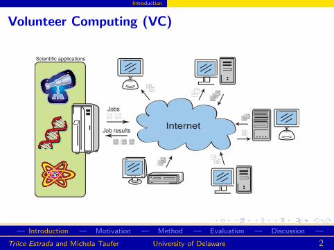
Volunteer Computing (VC)

Jobs

Job resultsInternet

Scientific applications

— Introduction — Motivation — Method — Evaluation — Discussion —..

Trilce Estrada and Michela Taufer University of Delaware 2

Introduction

Self-management in VC and in other distributed

systems

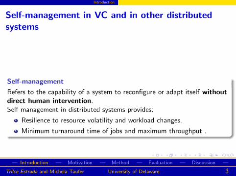
Self-management

Refers to the capability of a system to reconfigure or adapt itself withoutdirect human intervention.Self management in distributed systems provides:

Resilience to resource volatility and workload changes.

Minimum turnaround time of jobs and maximum throughput .

— Introduction — Motivation — Method — Evaluation — Discussion —..

Trilce Estrada and Michela Taufer University of Delaware 3

Introduction

Diversity of goals in VC scientific applications

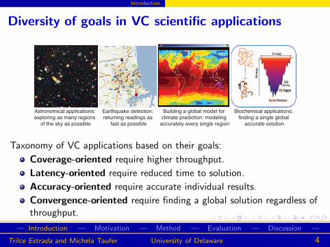
Biochemical applications:

finding a single global

accurate solution

Astronomical applications:

exploring as many regions

of the sky as possible

Earthquake detection:

returning readings as

fast as possible

Building a global model for

climate prediction: modeling

accurately every single region

Taxonomy of VC applications based on their goals:

Coverage-oriented require higher throughput.

Latency-oriented require reduced time to solution.

Accuracy-oriented require accurate individual results.

Convergence-oriented require finding a global solution regardless ofthroughput.

— Introduction — Motivation — Method — Evaluation — Discussion —..

Trilce Estrada and Michela Taufer University of Delaware 4

Introduction

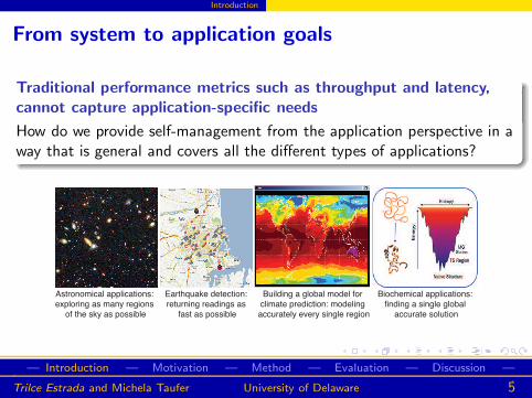
From system to application goals

Traditional performance metrics such as throughput and latency,cannot capture application-specific needs

How do we provide self-management from the application perspective in away that is general and covers all the different types of applications?

Biochemical applications:

finding a single global

accurate solution

Astronomical applications:

exploring as many regions

of the sky as possible

Earthquake detection:

returning readings as

fast as possible

Building a global model for

climate prediction: modeling

accurately every single region

— Introduction — Motivation — Method — Evaluation — Discussion —..

Trilce Estrada and Michela Taufer University of Delaware 5

Introduction

Outline

1 Introduction

2 MotivationChallenges of parametric scientific applicationsNeed for application-aware self-managed systems

3 MethodTowards a general application-aware self-managed VC systemUsing KOtrees for parameter prediction and explorationIntegrated modular framework

4 EvaluationDescriptionResults

5 DiscussionRelated workConclusion

— Introduction — Motivation — Method — Evaluation — Discussion —..

Trilce Estrada and Michela Taufer University of Delaware 6

Motivation

1 Introduction

2 MotivationChallenges of parametric scientific applicationsNeed for application-aware self-managed systems

3 MethodTowards a general application-aware self-managed VC systemUsing KOtrees for parameter prediction and explorationIntegrated modular framework

4 EvaluationDescriptionResults

5 DiscussionRelated workConclusion

— Introduction — Motivation — Method — Evaluation — Discussion —..

Trilce Estrada and Michela Taufer University of Delaware 7

Motivation Challenges of parametric scientific applications

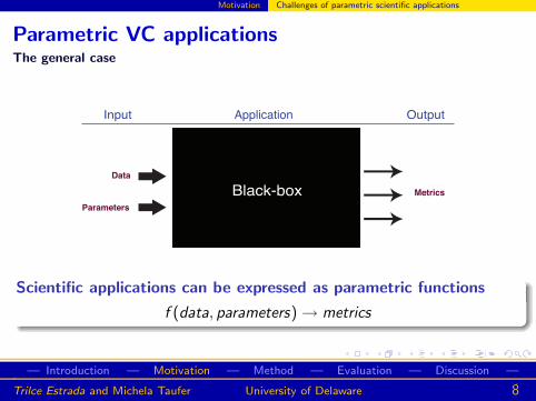
Parametric VC applicationsThe general case

Input Output

Data

Parameters

Metrics

Application

Black-box

Scientific applications can be expressed as parametric functions

f (data, parameters) → metrics

— Introduction — Motivation — Method — Evaluation — Discussion —..

Trilce Estrada and Michela Taufer University of Delaware 8

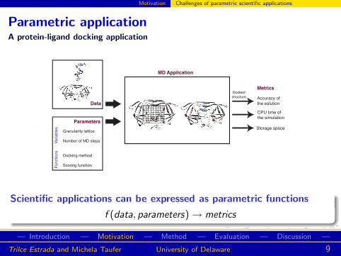
Motivation Challenges of parametric scientific applications

Parametric applicationA protein-ligand docking application

Data

Parameters

Granularity lattice

Number of MD steps

Docking method

Scoring function

Va

ria

ble

sF

un

ctio

ns

Docked

structure

Storage space

Accuracy of

the solution

CPU time of

the simulation

Metrics

MD Application

Scientific applications can be expressed as parametric functions

f (data, parameters) → metrics

— Introduction — Motivation — Method — Evaluation — Discussion —..

Trilce Estrada and Michela Taufer University of Delaware 9

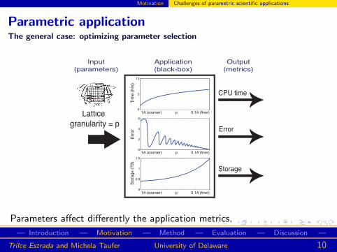
Motivation Challenges of parametric scientific applications

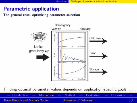
Parametric applicationThe general case: optimizing parameter selection

Lattice

granularity = p

CPU time

Error

Storage

0

0.5

1

1.5

Sto

rag

e (

TB

)

0

5

10

Tim

e (

hrs

)

0

2

4

6

Err

or

1A (coarser) p 0.1A (finer)

1A (coarser) p 0.1A (finer)

1A (coarser) p 0.1A (finer)

Input

(parameters)

Application

(black-box)

Output

(metrics)

Parameters affect differently the application metrics.

— Introduction — Motivation — Method — Evaluation — Discussion —..

Trilce Estrada and Michela Taufer University of Delaware 10

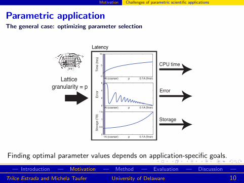
Motivation Challenges of parametric scientific applications

Parametric applicationThe general case: optimizing parameter selection

Lattice

granularity = p

CPU time

Error

Storage

Latency

0

0.5

1

1.5

Sto

rag

e (

TB

)

0

5

10

Tim

e (

hrs

)

0

2

4

6

Err

or

1A (coarser) p 0.1A (finer)

1A (coarser) p 0.1A (finer)

1A (coarser) p 0.1A (finer)

1A (coarser) p 0.1A (finer)

1A (coarser) p 0.1A (finer)

Finding optimal parameter values depends on application-specific goals.

— Introduction — Motivation — Method — Evaluation — Discussion —..

Trilce Estrada and Michela Taufer University of Delaware 10

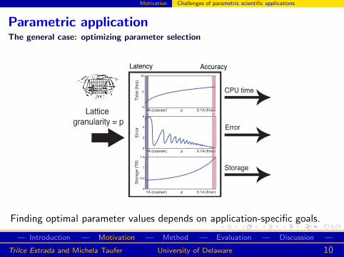
Motivation Challenges of parametric scientific applications

Parametric applicationThe general case: optimizing parameter selection

Lattice

granularity = p

CPU time

Error

Storage

Latency Accuracy

0

0.5

1

1.5

Sto

rag

e (

TB

)

0

5

10

Tim

e (

hrs

)

0

2

4

6

Err

or

1A (coarser) p 0.1A (finer)

1A (coarser) p 0.1A (finer)

1A (coarser) p 0.1A (finer)

1A (coarser) p 0.1A (finer)

1A (coarser) p 0.1A (finer)

1A (coarser) p 0.1A (finer)

1A (coarser) p 0.1A (finer)

Finding optimal parameter values depends on application-specific goals.

— Introduction — Motivation — Method — Evaluation — Discussion —..

Trilce Estrada and Michela Taufer University of Delaware 10

Motivation Challenges of parametric scientific applications

Parametric applicationThe general case: optimizing parameter selection

Lattice

granularity = p

CPU time

Error

Storage

Latency Accuracy

Convergency

0

0.5

1

1.5

Sto

rag

e (

TB

)

0

5

10

Tim

e (

hrs

)

0

2

4

6

Err

or

1A (coarser) p 0.1A (finer)

1A (coarser) p 0.1A (finer)

1A (coarser) p 0.1A (finer)

1A (coarser) p 0.1A (finer)

1A (coarser) p 0.1A (finer)

1A (coarser) p 0.1A (finer)

1A (coarser) p 0.1A (finer)

1A (coarser) p 0.1A (finer)

1A (coarser) p 0.1A (finer)

Finding optimal parameter values depends on application-specific goals.

— Introduction — Motivation — Method — Evaluation — Discussion —..

Trilce Estrada and Michela Taufer University of Delaware 10

Motivation Need for application-aware self-managed systems

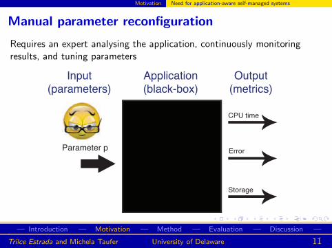
Manual parameter reconfiguration

Requires an expert analysing the application, continuously monitoringresults, and tuning parameters

Input

(parameters)

Application

(black-box)

Output

(metrics)

Parameter p

CPU time

Error

Storage

— Introduction — Motivation — Method — Evaluation — Discussion —..

Trilce Estrada and Michela Taufer University of Delaware 11

Motivation Need for application-aware self-managed systems

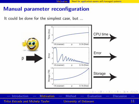
Manual parameter reconfiguration

It could be done for the simplest case, but ...

p

CPU time

Error

Storage

0

0.5

1

1.5

Sto

rag

e (

TB

)

0

5

10

Tim

e (

hrs

)

0

2

4

6E

rro

r

1A (coarser) p 0.1A (finer)

1A (coarser) p 0.1A (finer)

1A (coarser) p 0.1A (finer)

— Introduction — Motivation — Method — Evaluation — Discussion —..

Trilce Estrada and Michela Taufer University of Delaware 11

Motivation Need for application-aware self-managed systems

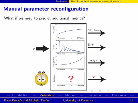
Manual parameter reconfiguration

What if we need to predict additional metrics?

p

CPU time

Error

Storage

0

0.5

1

1.5

Sto

rag

e (

TB

)

0

5

10

Tim

e (

hrs

)0

2

4

6

Err

or

1A (coarser) p 0.1A (finer)

1A (coarser) p 0.1A (finer)

1A (coarser) p 0.1A (finer)

Ba

nd

wid

th

1A (coarser) p 0.1A (finer)

? ?

— Introduction — Motivation — Method — Evaluation — Discussion —..

Trilce Estrada and Michela Taufer University of Delaware 11

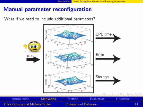
Motivation Need for application-aware self-managed systems

Manual parameter reconfiguration

What if we need to include additional parameters?

p, q

CPU time

Error

Storage

010

2030

010

2030

1

5

10

Tim

e (

hrs

)

010

2030

010

2030

0.5

1

1.5

Sto

rage

(T

B)

Err

or

010

2030

010

2030

−10

0

10

p

p

p

q

q

q

— Introduction — Motivation — Method — Evaluation — Discussion —..

Trilce Estrada and Michela Taufer University of Delaware 11

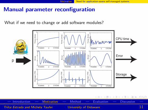
Motivation Need for application-aware self-managed systems

Manual parameter reconfiguration

What if we need to change or add software modules?

p

CPU time

Error

Storage

0

0.5

1

1.5

Sto

ra

ge

(T

B)

0

5

10

Tim

e (

hrs)

0

2

4

6

Erro

r

1A (coarser) p 0.1A (finer)

1A (coarser) p 0.1A (finer)

1A (coarser) p 0.1A (finer)

1

2

3

Tim

e (

hrs)

1A (coarser) p 0.1A (finer)

0.5

1

1.5

Erro

r

1A (coarser) p 0.1A (finer)

2

4

6

Sto

ra

ge

(T

B)

1A (coarser) p 0.1A (finer)

1

2

3

0

0.5

1

1.5

0

0.5

1

1.5

Tim

e (

hrs)

Erro

r1A (coarser) p 0.1A (finer)

Sto

ra

ge

(T

B)

1A (coarser) p 0.1A (finer)

1A (coarser) p 0.1A (finer)

— Introduction — Motivation — Method — Evaluation — Discussion —..

Trilce Estrada and Michela Taufer University of Delaware 11

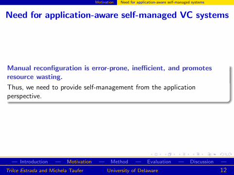
Motivation Need for application-aware self-managed systems

Need for application-aware self-managed VC systems

Manual reconfiguration is error-prone, inefficient, and promotesresource wasting.

Thus, we need to provide self-management from the applicationperspective.

— Introduction — Motivation — Method — Evaluation — Discussion —..

Trilce Estrada and Michela Taufer University of Delaware 12

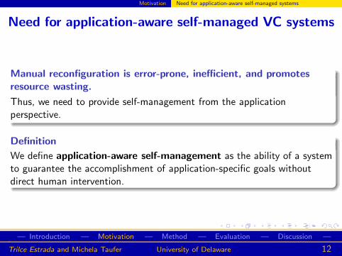
Motivation Need for application-aware self-managed systems

Need for application-aware self-managed VC systems

Manual reconfiguration is error-prone, inefficient, and promotesresource wasting.

Thus, we need to provide self-management from the applicationperspective.

Definition

We define application-aware self-management as the ability of a systemto guarantee the accomplishment of application-specific goals withoutdirect human intervention.

— Introduction — Motivation — Method — Evaluation — Discussion —..

Trilce Estrada and Michela Taufer University of Delaware 12

Method

1 Introduction

2 MotivationChallenges of parametric scientific applicationsNeed for application-aware self-managed systems

3 MethodTowards a general application-aware self-managed VC systemUsing KOtrees for parameter prediction and explorationIntegrated modular framework

4 EvaluationDescriptionResults

5 DiscussionRelated workConclusion

— Introduction — Motivation — Method — Evaluation — Discussion —..

Trilce Estrada and Michela Taufer University of Delaware 13

Method Towards a general application-aware self-managed VC system

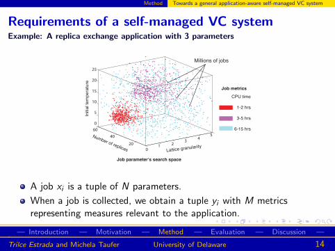
Requirements of a self-managed VC systemExample: A replica exchange application with 3 parameters

Number of replicas Lattice granularity

Initia

l te

mp

era

ture

01 2

34

5

Millions of jobs

25

20

15

10

5

0

60

40

20

CPU time

1-2 hrs

3-5 hrs

6-15 hrs

Job parameter’s search space

Job metrics

A job xi is a tuple of N parameters.

When a job is collected, we obtain a tuple yi with M metricsrepresenting measures relevant to the application.

— Introduction — Motivation — Method — Evaluation — Discussion —..

Trilce Estrada and Michela Taufer University of Delaware 14

Method Towards a general application-aware self-managed VC system

Requirements of a self-managed VC system

Number of replicas Lattice granularity

Initia

l te

mp

era

ture

01 2

34

5

25

20

15

10

5

0

60

40

20

Model

Use model

Build/update

model

Generate jobs

Collect jobs

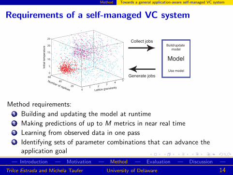
Method requirements:1 Building and updating the model at runtime2 Making predictions of up to M metrics in near real time3 Learning from observed data in one pass4 Identifying sets of parameter combinations that can advance the

application goal

— Introduction — Motivation — Method — Evaluation — Discussion —..

Trilce Estrada and Michela Taufer University of Delaware 14

Method Towards a general application-aware self-managed VC system

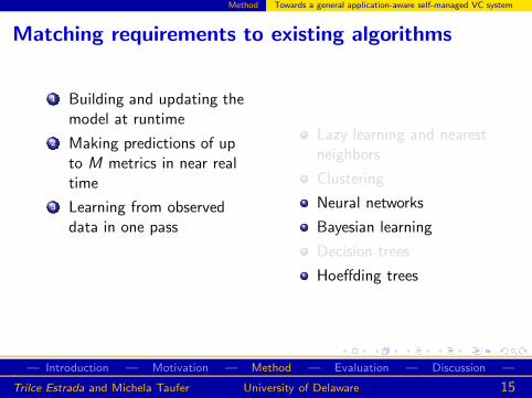
Matching requirements to existing algorithms

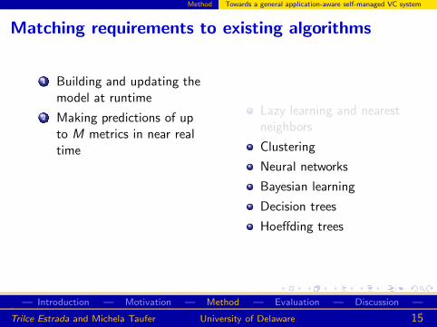
1 Building and updating themodel at runtime

Lazy learning and nearestneighbors

Clustering

Neural networks

Bayesian learning

Decision trees

Hoeffding trees

— Introduction — Motivation — Method — Evaluation — Discussion —..

Trilce Estrada and Michela Taufer University of Delaware 15

Method Towards a general application-aware self-managed VC system

Matching requirements to existing algorithms

1 Building and updating themodel at runtime

2 Making predictions of upto M metrics in near realtime

Lazy learning and nearestneighbors

Clustering

Neural networks

Bayesian learning

Decision trees

Hoeffding trees

— Introduction — Motivation — Method — Evaluation — Discussion —..

Trilce Estrada and Michela Taufer University of Delaware 15

Method Towards a general application-aware self-managed VC system

Matching requirements to existing algorithms

1 Building and updating themodel at runtime

2 Making predictions of upto M metrics in near realtime

3 Learning from observeddata in one pass

Lazy learning and nearestneighbors

Clustering

Neural networks

Bayesian learning

Decision trees

Hoeffding trees

— Introduction — Motivation — Method — Evaluation — Discussion —..

Trilce Estrada and Michela Taufer University of Delaware 15

Method Towards a general application-aware self-managed VC system

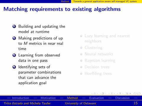
Matching requirements to existing algorithms

1 Building and updating themodel at runtime

2 Making predictions of upto M metrics in near realtime

3 Learning from observeddata in one pass

4 Identifying sets ofparameter combinationsthat can advance theapplication goal

Lazy learning and nearestneighbors

Clustering

Neural networks

Bayesian learning

Decision trees

Hoeffding trees

— Introduction — Motivation — Method — Evaluation — Discussion —..

Trilce Estrada and Michela Taufer University of Delaware 15

Method Using KOtrees for parameter prediction and exploration

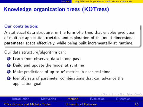
Knowledge organization trees (KOTrees)

Our contribution:

A statistical data structure, in the form of a tree, that enables predictionof multiple application metrics and exploration of the multi-dimensionalparameter space effectively, while being built incrementally at runtime.

Our data structure/algorithm can:

1 Learn from observed data in one pass

2 Build and update the model at runtime

3 Make predictions of up to M metrics in near real time

4 Identify sets of parameter combinations that can advance theapplication goal

— Introduction — Motivation — Method — Evaluation — Discussion —..

Trilce Estrada and Michela Taufer University of Delaware 16

Method Using KOtrees for parameter prediction and exploration

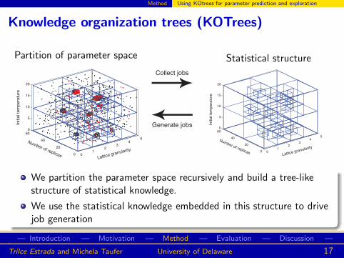
Knowledge organization trees (KOTrees)

Partition of parameter space

01

23

45

0

20

40

600

5

10

15

20

Number of replicasLattice granularity

Initia

l te

mp

era

ture

Generate jobs

Collect jobs

Statistical structure

01

23

45

0

20

40

600

5

10

15

20

Number of replicasLattice granularity

Initia

l te

mp

era

ture

We partition the parameter space recursively and build a tree-likestructure of statistical knowledge.

We use the statistical knowledge embedded in this structure to drivejob generation

— Introduction — Motivation — Method — Evaluation — Discussion —..

Trilce Estrada and Michela Taufer University of Delaware 17

Method Using KOtrees for parameter prediction and exploration

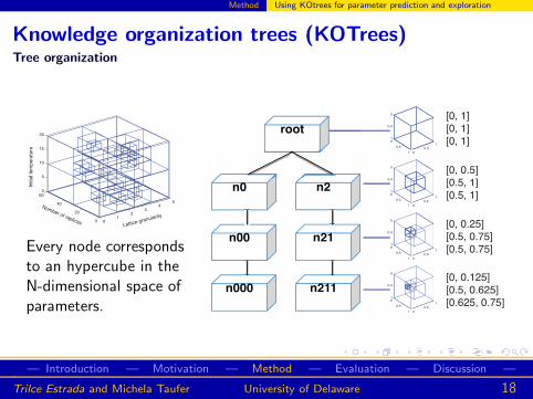
Knowledge organization trees (KOTrees)Tree organization

01

23

45

0

20

40

600

5

10

15

20

Number of replicasLattice granularity

Initia

l te

mp

era

ture

Every node correspondsto an hypercube in theN-dimensional space ofparameters.

0

0.5

1

1

0.5

01

0.5

0

0

0.5

1

1

0.5

01

0.5

0

0

0.5

1

1

0.5

01

0.5

0

0

0.5

1

1

0.5

01

0.5

0

[0, 1]

[0, 1]

[0, 1]

[0, 0.5]

[0.5, 1]

[0.5, 1]

[0, 0.25]

[0.5, 0.75]

[0.5, 0.75]

[0, 0.125]

[0.5, 0.625]

[0.625, 0.75]

root

n0

n00

n000

n2

n21

n211

— Introduction — Motivation — Method — Evaluation — Discussion —..

Trilce Estrada and Michela Taufer University of Delaware 18

Method Using KOtrees for parameter prediction and exploration

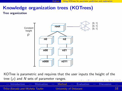
Knowledge organization trees (KOTrees)Tree organization

0

0.5

1

1

0.5

01

0.5

0 [0, 1]

[0, 1]

[0, 1]

ρ

Constant

height

root

n0

n00

n000

n2

n21

n211

KOTree is parametric and requires that the user inputs the height of thetree (ρ) and N sets of parameter ranges.

— Introduction — Motivation — Method — Evaluation — Discussion —..

Trilce Estrada and Michela Taufer University of Delaware 18

Method Using KOtrees for parameter prediction and exploration

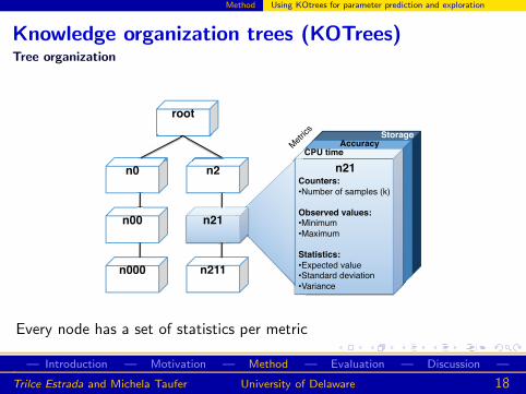
Knowledge organization trees (KOTrees)Tree organization

n21Counters:

•Number of samples (k)

Observed values:•Minimum

•Maximum

Statistics:

•Expected value•Standard deviation

•Variance

CPU timeAccuracy

Storage

Met

rics

root

n0

n00

n000

n2

n21

n211

Every node has a set of statistics per metric

— Introduction — Motivation — Method — Evaluation — Discussion —..

Trilce Estrada and Michela Taufer University of Delaware 18

Method Using KOtrees for parameter prediction and exploration

Requirement 1: One-pass learning

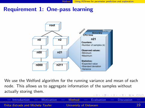
n21Counters:

•Number of samples (k)

Observed values:•Minimum

•Maximum

Statistics:

•Expected value•Standard deviation

•Variance

CPU timeAccuracy

Storage

Met

rics

root

n0

n00

n000

n2

n21

n211

We use the Welford algorithm for the running variance and mean of eachnode. This allows us to aggregate information of the samples withoutactually storing them.

— Introduction — Motivation — Method — Evaluation — Discussion —..

Trilce Estrada and Michela Taufer University of Delaware 19

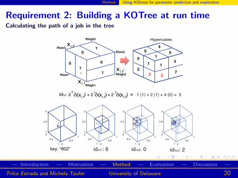
Method Using KOtrees for parameter prediction and exploration

Requirement 2: Building a KOTree at run timeCalculating the path of a job in the tree

0

1

2

3

1

3

5

7

4

51

0

01

0

1

01

Rlow1

Rhigh1

Rlow2

Rhigh2

Rlow3

Rhigh3

x i,3

22 + 2 + 2

10δ( ) δ( ) δ( ) 1 (1) + 2 (1) + 4 (0) = 3=

Hypercubes

idhc:

x i,2

x i,1

xi,3xi,2xi,1

0

0.5

1

1

0.5

01

0.5

0

0

0.5

1

1

0.5

01

0.5

0

0

0.5

1

1

0.5

01

0.5

0

0

0.5

1

1

0.5

01

0.5

0

idhc1: 6 idhc2: 0 idhc3: 2key: “602”

xi

— Introduction — Motivation — Method — Evaluation — Discussion —..

Trilce Estrada and Michela Taufer University of Delaware 20

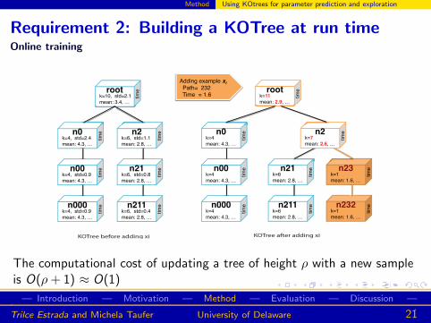
Method Using KOtrees for parameter prediction and exploration

Requirement 2: Building a KOTree at run timeOnline training

KOTree before adding xi KOTree after adding xi

n0k=4

mean: 4.3, …

tim

e

n00k=4

mean: 4.3, …

tim

e

n000k=4

mean: 4.3, …

tim

e

rootk=11

mean: 2.9, …

tim

e

n21k=6

mean: 2.8, …

tim

e

n211k=6

mean: 2.8, …

tim

e

n23k=1

mean: 1.6, …

tim

e

n232k=1

mean: 1.6, …

tim

e

n2k=7

mean: 2.6, …

tim

e

Adding example xi Path= 232 Time = 1.6

rootk=10, std=2.1

mean: 3.4, …

tim

en0

k=4, std=2.4

mean: 4.3, …

tim

e

n00k=4, std=0.9

mean: 4.3, …

tim

e

n000k=4, std=0.9

mean: 4.3, …

tim

e

n2k=6, std=1.1

mean: 2.8, …

tim

e

n21k=6, std=0.8

mean: 2.8, …

tim

e

n211k=6, std=0.4

mean: 2.8, …

tim

e

The computational cost of updating a tree of height ρ with a new sampleis O(ρ + 1) ≈ O(1)

— Introduction — Motivation — Method — Evaluation — Discussion —..

Trilce Estrada and Michela Taufer University of Delaware 21

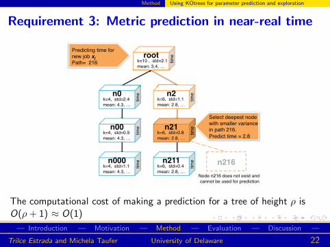
Method Using KOtrees for parameter prediction and exploration

Requirement 3: Metric prediction in near-real time

rootk=10 , std=2.1

mean: 3.4, …

tim

e

n0k=4, std=2.4

mean: 4.3, …

tim

e

n00k=4, std=0.9

mean: 4.3, …tim

e

n000k=4, std=1.1

mean: 4.3, …

tim

e

n2k=6, std=1.1

mean: 2.8, …

tim

e

n21k=6, std=0.8

mean: 2.8, …

tim

e

n211k=6, std=0.4

mean: 2.8, …

tim

e n216

Predicting time fornew job xj Path= 216

tim

e

Select deepest node with smaller variancein path 216.

Predict time = 2.8

Node n216 does not exist and

cannot be used for prediction

The computational cost of making a prediction for a tree of height ρ isO(ρ + 1) ≈ O(1)

— Introduction — Motivation — Method — Evaluation — Discussion —..

Trilce Estrada and Michela Taufer University of Delaware 22

Method Using KOtrees for parameter prediction and exploration

Requirement 4: Parameter space exploration

The statistical structure in KOTree can find sweet-spots of parameterswhose jobs can potentially advance application goals

01

23

45

0

20

40

600

5

10

15

20

Number of replicasLattice granularity

Initia

l te

mp

era

ture

— Introduction — Motivation — Method — Evaluation — Discussion —..

Trilce Estrada and Michela Taufer University of Delaware 23

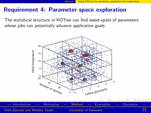
Method Using KOtrees for parameter prediction and exploration

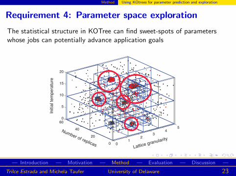
Requirement 4: Parameter space exploration

The statistical structure in KOTree can find sweet-spots of parameterswhose jobs can potentially advance application goals

01

23

45

0

20

40

600

5

10

15

20

Number of replicasLattice granularity

Initia

l te

mp

era

ture

— Introduction — Motivation — Method — Evaluation — Discussion —..

Trilce Estrada and Michela Taufer University of Delaware 23

Method Using KOtrees for parameter prediction and exploration

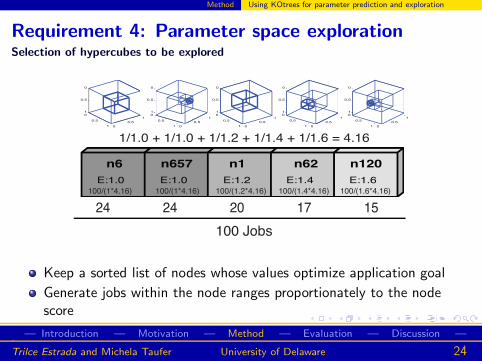
Requirement 4: Parameter space explorationSelection of hypercubes to be explored

24 24 20 17 15

100 Jobs

n6 n657 n1 n62 n120

E:1.0 E:1.0 E:1.2 E:1.4 E:1.6

0

0.5

1

1

0.5

01

0.5

0

0

0.5

1

1

0.5

01

0.5

0

0

0.5

1

1

0.5

01

0.5

0

0

0.5

1

1

0.5

01

0.5

0

0

0.5

1

1

0.5

01

0.5

0

100/(1*4.16) 100/(1.2*4.16) 100/(1.6*4.16)

1/1.0 + 1/1.0 + 1/1.2 + 1/1.4 + 1/1.6 = 4.16

100/(1*4.16) 100/(1.4*4.16)

Keep a sorted list of nodes whose values optimize application goal

Generate jobs within the node ranges proportionately to the nodescore

— Introduction — Motivation — Method — Evaluation — Discussion —..

Trilce Estrada and Michela Taufer University of Delaware 24

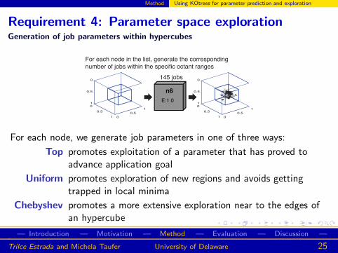
Method Using KOtrees for parameter prediction and exploration

Requirement 4: Parameter space explorationGeneration of job parameters within hypercubes

n6

E:1.0

0

0.5

1

1

0.5

01

0.5

0

For each node in the list, generate the corresponding

number of jobs within the specific octant ranges

0

0.5

1

1

0.5

01

0.5

0145 jobs

For each node, we generate job parameters in one of three ways:

Top promotes exploitation of a parameter that has proved toadvance application goal

Uniform promotes exploration of new regions and avoids gettingtrapped in local minima

Chebyshev promotes a more extensive exploration near to the edges ofan hypercube

— Introduction — Motivation — Method — Evaluation — Discussion —..

Trilce Estrada and Michela Taufer University of Delaware 25

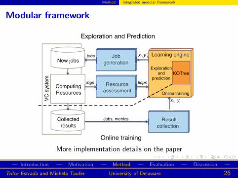
Method Integrated modular framework

Modular framework

KOTree

Result

collection

Resource

assessment

Job

generation

Learning engine

Collected

results

New jobs

Computing

Resources Online training

Explorationand

prediction

VC

syste

m

Online training

Exploration and Prediction

Jobs, metrics

jobs

xi , yi

xi ,y i

flopslogs

Job

generation

Resource

assessment

Result

collection

More implementation details on the paper

— Introduction — Motivation — Method — Evaluation — Discussion —..

Trilce Estrada and Michela Taufer University of Delaware 26

Evaluation

1 Introduction

2 MotivationChallenges of parametric scientific applicationsNeed for application-aware self-managed systems

3 MethodTowards a general application-aware self-managed VC systemUsing KOtrees for parameter prediction and explorationIntegrated modular framework

4 EvaluationDescriptionResults

5 DiscussionRelated workConclusion

— Introduction — Motivation — Method — Evaluation — Discussion —..

Trilce Estrada and Michela Taufer University of Delaware 27

Evaluation Description

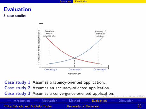
Evaluation3 case studies

(-)

Re

leva

nce

fo

r th

e a

pp

lica

tio

n g

oa

l (+

)

Application goal

Execution

time of

individual jobs

Case study 2Case study 1 Case study 3

Accuracy of

individual

solutions

Case study 1 Assumes a latency-oriented application.

Case study 2 Assumes an accuracy-oriented application.

Case study 3 Assumes a convergence-oriented application.

— Introduction — Motivation — Method — Evaluation — Discussion —..

Trilce Estrada and Michela Taufer University of Delaware 28

Evaluation Description

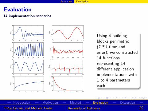
Evaluation14 implementation scenarios

0 1 2 3 4 50

2

4

6

Tim

e

0 1 2 3 4 50

0.5

1

1.5

Err

or

0 10 20 30 40 50 600

2

4

6

Tim

e

0 10 20 30 40 50 600

1

2

3

Err

or

0 5 10 15 200

1

2

3

Tim

e

0 5 10 15 200

0.5

1

1.5

Err

or

5 10 15 20 250

5

10

Tim

e

5 10 15 20 250

0.5

1

1.5

Err

or

Using 4 buildingblocks per metric(CPU time anderror), we constructed14 functionsrepresenting 14different applicationimplementations with1 to 4 parameterseach

— Introduction — Motivation — Method — Evaluation — Discussion —..

Trilce Estrada and Michela Taufer University of Delaware 29

Evaluation Description

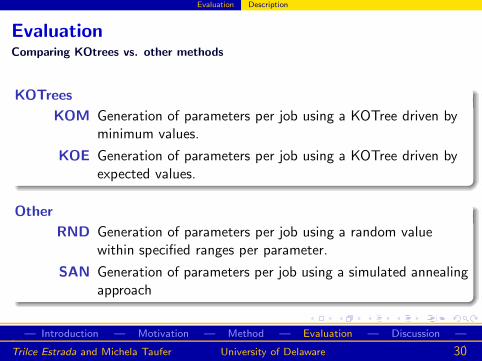
EvaluationComparing KOtrees vs. other methods

KOTrees

KOM Generation of parameters per job using a KOTree driven byminimum values.

KOE Generation of parameters per job using a KOTree driven byexpected values.

Other

RND Generation of parameters per job using a random valuewithin specified ranges per parameter.

SAN Generation of parameters per job using a simulated annealingapproach

— Introduction — Motivation — Method — Evaluation — Discussion —..

Trilce Estrada and Michela Taufer University of Delaware 30

Evaluation Description

EvaluationExperimental set-up

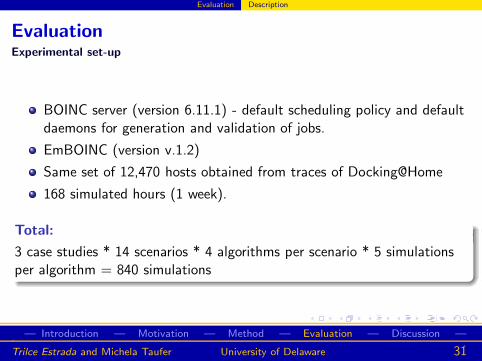
BOINC server (version 6.11.1) - default scheduling policy and defaultdaemons for generation and validation of jobs.

EmBOINC (version v.1.2)

Same set of 12,470 hosts obtained from traces of Docking@Home

168 simulated hours (1 week).

Total:

3 case studies * 14 scenarios * 4 algorithms per scenario * 5 simulationsper algorithm = 840 simulations

— Introduction — Motivation — Method — Evaluation — Discussion —..

Trilce Estrada and Michela Taufer University of Delaware 31

Evaluation Results

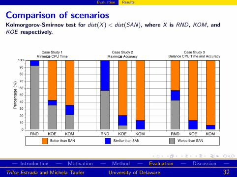
Comparison of scenariosKolmorgorov-Smirnov test for dist(X ) < dist(SAN), where X is RND, KOM, andKOE respectively.

RND KOE KOM RND KOE KOM RND KOE KOM0

10

20

30

40

50

60

70

80

90

100

Percentage (%)

Worse than SANSimilar than SANBetter than SAN

Case Study 1Minimize CPU Time

Case Study 2Maximize Accuracy

Case Study 3Balance CPU Time and Accuracy

— Introduction — Motivation — Method — Evaluation — Discussion —..

Trilce Estrada and Michela Taufer University of Delaware 32

Evaluation Results

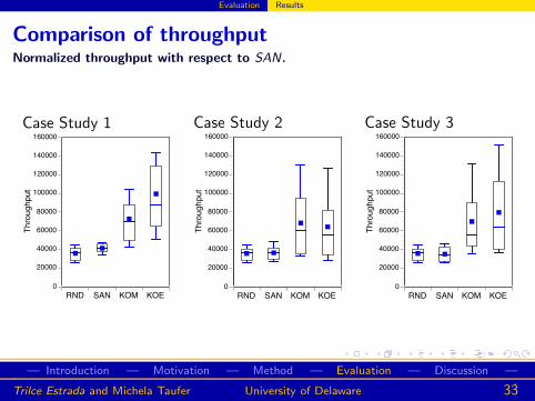
Comparison of throughputNormalized throughput with respect to SAN.

Case Study 1

BB

B

B

RND SAN KOM KOE0

20000

40000

60000

80000

100000

120000

140000

160000

Throughput

Case Study 2

B B

BB

RND SAN KOM KOE0

20000

40000

60000

80000

100000

120000

140000

160000

Throughput

Case Study 3

B B

B

B

RND SAN KOM KOE0

20000

40000

60000

80000

100000

120000

140000

160000

Throughput

— Introduction — Motivation — Method — Evaluation — Discussion —..

Trilce Estrada and Michela Taufer University of Delaware 33

Evaluation Results

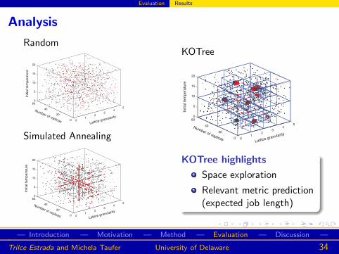
Analysis

Random

01

23

45

0

20

40

600

5

10

15

20

Number of replicasLattice granularity

Initia

l te

mp

era

ture

Simulated Annealing

01

23

45

0

20

40

600

5

10

15

20

Number of replicasLattice granularity

Initia

l te

mp

era

ture

KOTree

01

23

45

0

20

40

600

5

10

15

20

Number of replicasLattice granularity

Initia

l te

mp

era

ture

KOTree highlights

Space exploration

Relevant metric prediction(expected job length)

— Introduction — Motivation — Method — Evaluation — Discussion —..

Trilce Estrada and Michela Taufer University of Delaware 34

Discussion

1 Introduction

2 MotivationChallenges of parametric scientific applicationsNeed for application-aware self-managed systems

3 MethodTowards a general application-aware self-managed VC systemUsing KOtrees for parameter prediction and explorationIntegrated modular framework

4 EvaluationDescriptionResults

5 DiscussionRelated workConclusion

— Introduction — Motivation — Method — Evaluation — Discussion —..

Trilce Estrada and Michela Taufer University of Delaware 35

Discussion Related work

Related work

Build and update a tree-like model at runtime, which is able to learnfrom observed data in a single pass, can be used to predict multipleapplication metrics and explore parameter spaces efficiently.

Stream mining algorithms [Guha et.al., Zhang et.al., Yang et.al., Uenoet.al., He et.al., Leng et.al., Raahemi et.al., Kawashima et.al., Qinget.al., Machot et.al., Domingos et.al.]

Build a modular framework allowing integration of application-awareself-management in VC.

MindModeling@Home propose the Cell mechanism to exploreparameter space [Moore Jr. et.al.]

— Introduction — Motivation — Method — Evaluation — Discussion —..

Trilce Estrada and Michela Taufer University of Delaware 36

Discussion Conclusion

Conclusion

We present an autonomic, modular framework for providingapplication-aware self-management for VC applications

KOTree is a fully automatic method that can be built and updated atruntime. At any point in time, we have an organized data structure thatcan predict multiple metrics of interest and explore the N-dimensional

space of parameters effectively.

This framework can effectively provide application-awareself-management in VC systems.

The KOTree algorithm is able to predict expected length of new jobsaccurately, resulting in an average of 85% increased throughput withrespect to other algorithms.

— Introduction — Motivation — Method — Evaluation — Discussion —..

Trilce Estrada and Michela Taufer University of Delaware 37

Acknowledgements

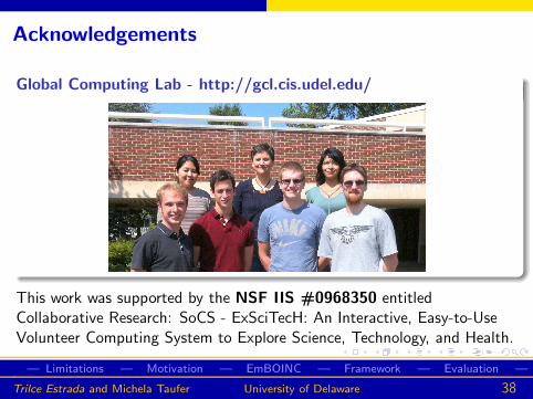
Global Computing Lab - http://gcl.cis.udel.edu/

This work was supported by the NSF IIS #0968350 entitledCollaborative Research: SoCS - ExSciTecH: An Interactive, Easy-to-UseVolunteer Computing System to Explore Science, Technology, and Health.

— Limitations — Motivation — EmBOINC — Framework — Evaluation —..

Trilce Estrada and Michela Taufer University of Delaware 38

Questions

Contact

Trilce Estrada, estrada@udel.edu

Michela Taufer, taufer@udel.edu

— Limitations — Motivation — EmBOINC — Framework — Evaluation —..

Trilce Estrada and Michela Taufer University of Delaware 39

Future directions

Future work

Adding a range expansion mechanism that allows just a roughestimate of the initial parameter space.

Extending our application-aware self-management framework to otherdistributed systems.

Extending KOTrees to perform multi-classification in the context of ageneral stream mining algorithm

— Limitations — Motivation — EmBOINC — Framework — Evaluation —..

Trilce Estrada and Michela Taufer University of Delaware 40

Limitations

LimitationsParametric nature of KOTree

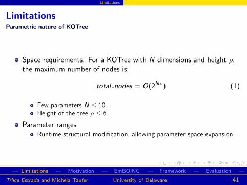
Space requirements. For a KOTree with N dimensions and height ρ,the maximum number of nodes is:

total nodes = O(2Nρ) (1)

Few parameters N ≤ 10Height of the tree ρ ≤ 6

Parameter ranges

Runtime structural modification, allowing parameter space expansion

— Limitations — Motivation — EmBOINC — Framework — Evaluation —..

Trilce Estrada and Michela Taufer University of Delaware 41

Limitations Range expansion

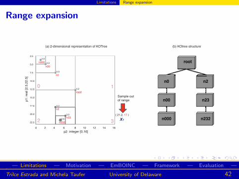
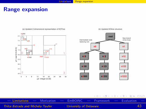
Range expansion

(b) KOtree structure (a) 2-dimensional representation of KOTree

root

n0

n00

n000

n2

n23

n232

4.2

3.2

3.0

2.6

5.3

4.3

4.3

0 1

2 3

root

n0

n00

n000

n2

n23

n232

0 2 4 6 8 10 12 14 16

2.5

5.0

7.5

10.0

12.5

15.0

17.5

20.0

22.5

p1

: re

al [2

.5,2

2.5

]

p2: integer [0,16]

X1

( 21.2, 17 )

Sample out

of range

— Limitations — Motivation — EmBOINC — Framework — Evaluation —..

Trilce Estrada and Michela Taufer University of Delaware 42

Limitations Range expansion

Range expansion

root

n00

n000

n0000

n02

n023

n0232

n12

n122

n1222

n0 n1

0 4 8 12 16 20 24 28 32

2.5

7.5

12.5

17.5

22.5

27.0

32.5

37.5

42.5

p2: integer [0,32]

p1

: re

al [2

.5,4

2.5

]

0 1

2 3

root

n000

n00

n0

n02

n023

n0232

n0000

n1

n12

n122

n1222

(b) Updated KOtree structure (a) Updated 2-dimensional representation of KOTree

Intermediate node

replacing root

New branch

of the three

— Limitations — Motivation — EmBOINC — Framework — Evaluation —..

Trilce Estrada and Michela Taufer University of Delaware 43

Motivation

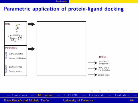
Parametric application of protein-ligand docking

Data

Parameters

Granularity lattice

Number of MD steps

Docking method

Scoring function

Va

ria

ble

sF

un

ctio

ns

Storage space

Accuracy of

the solution

CPU time of

the simulation

Metrics

— Limitations — Motivation — EmBOINC — Framework — Evaluation —..

Trilce Estrada and Michela Taufer University of Delaware 44

Motivation

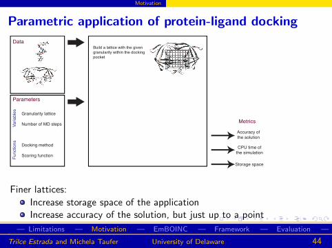
Parametric application of protein-ligand docking

Data

Parameters

Granularity lattice

Number of MD steps

Docking method

Scoring function

Build a lattice with the given

granularity within the docking

pocket

Va

ria

ble

sF

un

ctio

ns

Storage space

Accuracy of

the solution

CPU time of

the simulation

Metrics

Finer lattices:

Increase storage space of the applicationIncrease accuracy of the solution, but just up to a point

— Limitations — Motivation — EmBOINC — Framework — Evaluation —..

Trilce Estrada and Michela Taufer University of Delaware 44

Motivation

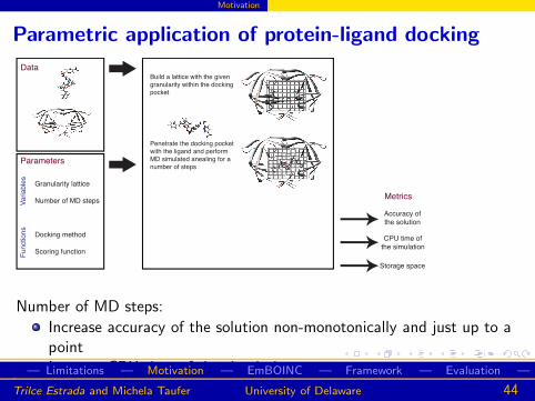
Parametric application of protein-ligand docking

Data

Parameters

Granularity lattice

Number of MD steps

Docking method

Scoring function

Build a lattice with the given

granularity within the docking

pocket

Penetrate the docking pocket

with the ligand and perform

MD simulated anealing for a

number of steps

Va

ria

ble

sF

un

ctio

ns

Storage space

Accuracy of

the solution

CPU time of

the simulation

Metrics

Number of MD steps:

Increase accuracy of the solution non-monotonically and just up to apointIncrease CPU time of the simulation— Limitations — Motivation — EmBOINC — Framework — Evaluation —.

.Trilce Estrada and Michela Taufer University of Delaware 44

Motivation

Parametric application of protein-ligand docking

Data

Parameters

Granularity lattice

Number of MD steps

Docking method

Scoring function

Build a lattice with the given

granularity within the docking

pocket

Penetrate the docking pocket

with the ligand and perform

MD simulated anealing for a

number of steps

Va

ria

ble

sF

un

ctio

ns

Storage space

Accuracy of

the solution

CPU time of

the simulation

MetricsUse the given docking method

to clacluate atomic interactions

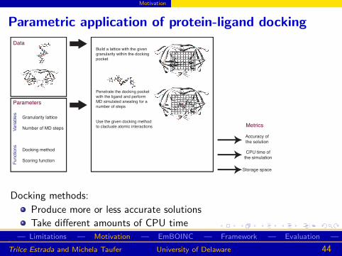
Docking methods:

Produce more or less accurate solutions

Take different amounts of CPU time— Limitations — Motivation — EmBOINC — Framework — Evaluation —.

.Trilce Estrada and Michela Taufer University of Delaware 44

Motivation

Parametric application of protein-ligand docking

Data

Parameters

Granularity lattice

Number of MD steps

Docking method

Scoring function

Build a lattice with the given

granularity within the docking

pocket

Penetrate the docking pocket

with the ligand and perform

MD simulated anealing for a

number of steps

Va

ria

ble

sF

un

ctio

ns

Determine how well the ligand

docked into the protein using

the scoring function

Docked

structure

Storage space

Accuracy of

the solution

CPU time of

the simulation

MetricsUse the given docking method

to clacluate atomic interactions

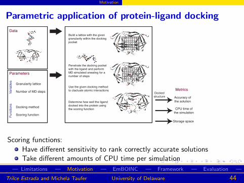
Scoring functions:

Have different sensitivity to rank correctly accurate solutionsTake different amounts of CPU time per simulation

— Limitations — Motivation — EmBOINC — Framework — Evaluation —..

Trilce Estrada and Michela Taufer University of Delaware 44

EmBOINC

Simulating multiscale applications with EmBOINC

p

p

p

p

p

p

p

p

p

scale 1 scale 2 scale 3

f1( ) + p , p , ..., p1 2 N

y

y

y

1

2

M

p , p , ..., p1 2 N

g1( ) +p , p , ..., p1 2 N

h1( ) p , p , ..., p1 2 N

f2( ) + p , p , ..., p1 2 N

g2( ) + p , p , ..., p1 2 N

h2( ) p , p , ..., p1 2 N

fM( ) + p , p , ..., p1 2 N

gM( ) + p , p , ..., p1 2 N

hM( ) p , p , ..., p1 2 N

Application

parameters

Application

metrics

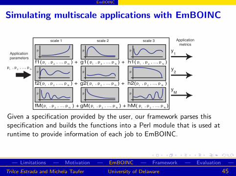
Given a specification provided by the user, our framework parses thisspecification and builds the functions into a Perl module that is used atruntime to provide information of each job to EmBOINC.

— Limitations — Motivation — EmBOINC — Framework — Evaluation —..

Trilce Estrada and Michela Taufer University of Delaware 45

EmBOINC

Simulating multiscale applications with EmBOINC

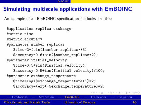
An example of an EmBOINC specification file looks like this:

@application replica_exchange

@metric time

@metric accuracy

@parameter number_replicas

$time=2+(sin($number_replicas**3);

$accuracy=0.6+sin($number_replicas*2);

@parameter initial_velocity

$time=0.5+sin($initial_velocity);

$accuracy=0.5+tan($initial_velocity)/100;

@parameter exchange_temperature

$time=log($exchange_temperature+1)*2;

$accuracy=(exp(-$exchange_temperature)*2;

— Limitations — Motivation — EmBOINC — Framework — Evaluation —..

Trilce Estrada and Michela Taufer University of Delaware 46

EmBOINC Exploration

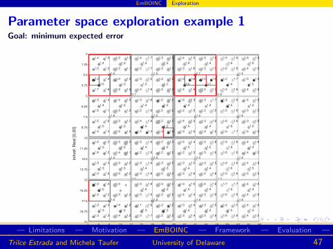
Parameter space exploration example 1Goal: minimum expected error

1 5 9 13 17 21 25 29 33 37 41 45 49 53 57 61 6520

18.75

17.5

16.25

15

13.75

12.5

11.25

10

8.75

7.5

6.25

5

3.75

2.5

1.25

0

0.7

0.5

0.5

0.5

1.5

1.3

1.3

1.3

1.1

1.1

1.3

1.2

1.2

1.3

1.3

1.3

1.4

1.5

1.4

1.4

1.5

1.4

1.5

1.3

1.4

1.4

1.5

1.3

1.3

1.6

1.6

1.6

0.8

1.5

1.6

1.7

1.5

1.6

1.4

1.4

0.7

0.7

0.8

1.4

1.4

1.5

1.4

1.4

1.2

1.3

1.2

1.2

1.4

1.4

1.3

1.2

1.2

1.3

1.1

1.3

1.5

1.6

1.6

1.6

1.4

1.7

1.4

1.5

1.5

1.5

1.4

1.7

1.2

1.3

1.4

1.21.4

1.3

1.3

1.3

1.3

1.4

1.3

1.3

1.0

1.0

1.2

1.5

1.3

1.6

1.4

1.3

1.3

1.4

1.6

1.5

1.6

1.4

1.4

1.6

1.0

1.6

1.3

1.5

1.5

1.5

1.5

1.4

0.9

1.41.3

1.4

1.4

1.6

1.7

1.6

1.6

1.6

1.5

1.5

1.6

1.4

1.5

1.3

1.2

1.3

1.5

1.3

1.3

1.2

1.3

1.2

1.3

1.5

1.6

1.5

1.6

1.5

1.6

1.6

1.2

1.7

1.6

1.3

1.3 1.2

1.4

1.3

1.3

1.2

1.2

1.21.3

1.4

1.3

1.6

1.6

1.5

1.4

1.5

1.6

1.3

1.4

1.3

1.6

0.5

1.4

1.4

1.5

1.3

1.2

1.3

1.4

1.4

1.6

1.4

1.4 1.4

1.3

1.3

1.7

1.3

1.3

1.4

1.4 1.6

1.6

1.5

1.3

1.2

1.4

1.4

1.5

1.5

1.3

1.6

1.2

1.2

1.6

1.6

1.4

1.3

1.2

1.4

1.3 1.2

1.2

1.2

1.3 1.3

1.5

1.5

1.6

1.5

1.4

1.3

1.6

1.5

1.6 1.1

1.3

1.3

1.3

1.3

1.6

1.3

1.6

1.6

1.4

1.1

1.3

1.4

1.4

1.6

1.2

1.3

1.3

1.3

1.3

1.3

1.5

1.4

1.6

1.3

1.5

1.31.4

1.4

1.2

1.3

1.2

1.2

1.3

1.4

1.5

1.7

1.5

1.6

1.5

1.3 1.3

1.2

1.4

1.3

1.5

1.6

1.6

1.3

1.2

1.2

1.2

1.2

1.3

1.2

1.2

1.3

1.4

1.5

1.3

1.6

1.5

1.2

1.6

1.7

1.4

1.5

1.2

1.4

1.5

1.5

1.3

1.3

1.0

1.3

1.2

1.5

1.6

0.6

1.3

1.3

1.6

1.2

1.3

1.2

1.3

1.3

1.2

1.4

1.6

1.6

1.2

1.6

1.3

1.6

1.4

1.5

1.3

1.7

1.3

1.4

1.2

1.2

1.2

1.6

1.6

1.6

1.6

1.6

1.2

1.5

1.3

1.3

1.3

1.5

1.2

1.5

1.4

1.5

initve

l: R

ea

l [0

,20

]

nreplicas: Integer [1,65]— Limitations — Motivation — EmBOINC — Framework — Evaluation —..

Trilce Estrada and Michela Taufer University of Delaware 47

EmBOINC Exploration

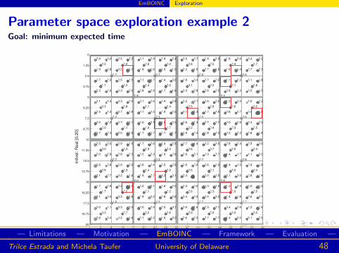
Parameter space exploration example 2Goal: minimum expected time

1 5 9 13 17 21 25 29 33 37 41 45 49 53 57 61 6520

18.75

17.5

16.25

15

13.75

12.5

11.25

10

8.75

7.5

6.25

5

3.75

2.5

1.25

0

1.8

1.7

1.7

1.7

2.2

2.1

1.7

2.4

1.3

2.0

2.3

2.6

1.6

2.1

2.0

1.9

2.8

2.9

3.3

2.9

2.7

3.2

2.5

2.5

2.7

2.1

2.0

2.2

2.5

3.0

3.5

1.4

2.3

2.6

2.3

2.2

2.0

2.2

2.5

2.9

2.3

2.2

2.0

2.5

2.5

1.3

3.3

4.3

2.6

2.3

2.3

1.4

2.7

2.9

3.7

2.0

3.0

2.2

2.0

1.6

3.0

1.4

2.0

1.4

2.6

1.6

2.4

2.3

1.9

2.0

2.8

3.0

2.0

2.3

1.9

1.72.4

2.2

1.5

2.4

1.4

2.7

2.3

3.2

1.8

1.7

2.1

2.6

1.3

2.7

3.1

3.1

2.7

3.3

3.7

2.9

2.1

2.2

2.6

2.6

1.7

2.5

2.6

3.9

2.1

2.5

2.7

2.7

3.1

3.32.3

2.5

2.3

2.6

2.2

2.7

3.0

4.7

3.0

2.2

2.0

2.1

2.9

2.2

3.1

2.1

2.5

2.4

3.1

1.8

1.9

2.3

2.9

2.8

2.4

1.9

3.5

2.8

1.5

1.8

3.4

1.3

1.4

2.9

3.8 2.0

2.6

2.1

2.3

2.0

2.5

1.8

2.2

3.3

2.5

2.7

2.9

2.2

2.7

4.2

3.7

3.0

2.6

2.5

2.6

3.7

2.7

4.0

1.7

2.4

2.1

3.1

3.2

4.1

2.3

3.3

2.6

3.4 2.0

2.8

1.8

2.2

3.3

3.0

2.8

3.5 3.6

3.6

2.0

2.7

2.9

2.9

2.3

2.4

1.4

4.3

2.4

2.4

1.9

3.3

1.6

2.4

1.9

1.1

2.1

1.9 2.6

1.7

2.3

2.6 2.6

2.8

2.8

3.3

2.8

2.8

1.6

2.3

3.0

3.0 2.3

2.2

1.7

1.3

2.7

2.0

2.4

3.3

1.8

3.5

4.3

2.9

2.5

2.0

3.2

1.0

2.8

3.6

1.8

1.8

2.9

2.3

1.7

4.2

3.3

2.0

1.8

2.93.3

1.6

1.8

4.1

2.4

2.5

1.7

4.1

2.8

2.9

1.0

3.4

2.2

3.4 2.6

2.9

2.6

2.2

1.8

3.7

3.4

2.6

1.0

3.1

2.3

2.9

2.0

1.2

2.2

1.5

3.1

2.9

1.9

4.3

3.1

3.5

3.0

3.4

1.7

2.9

2.8

2.9

2.5

2.7

3.2

2.3

1.7

1.3

1.8

2.4

2.7

3.3

2.6

1.9

2.9

3.5

2.7

3.3

3.4

2.5

1.5

2.3

3.9

1.4

1.6

2.1

2.1

3.6

2.8

3.1

2.7

2.2

2.2

1.4

1.9

2.1

2.8

2.2

1.6

1.9

3.2

1.8

1.6

1.7

2.1

2.3

2.7

2.0

3.4

1.6

1.3

initve

l: R

ea

l [0

,20

]

nreplicas: Integer [1,65]— Limitations — Motivation — EmBOINC — Framework — Evaluation —..

Trilce Estrada and Michela Taufer University of Delaware 48

Framework

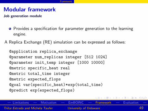
Modular frameworkJob generation module

Provides a specification for parameter generation to the learningengine.

A Replica Exchange (RE) simulation can be expressed as follows:

@application replica_exchange

@parameter num_replicas integer [512 1024]

@parameter init_temp integer [1000 10000]

@metric specific_heat real

@metric total_time integer

@metric expected_flops

@goal var(specific_heat)*exp(total_time)

@predict exp(expected_flops)

— Limitations — Motivation — EmBOINC — Framework — Evaluation —..

Trilce Estrada and Michela Taufer University of Delaware 49

Framework

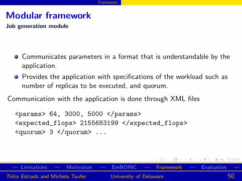
Modular frameworkJob generation module

Communicates parameters in a format that is understandable by theapplication.

Provides the application with specifications of the workload such asnumber of replicas to be executed, and quorum.

Communication with the application is done through XML files

<params> 64, 3000, 5000 </params>

<expected_flops> 2155683199 </expected_flops>

<quorum> 3 </quorum> ...

— Limitations — Motivation — EmBOINC — Framework — Evaluation —..

Trilce Estrada and Michela Taufer University of Delaware 50

Framework

Modular frameworkSystem assessment module

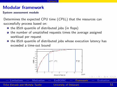
Determines the expected CPU time (CPUt) that the resources cansuccessfully process based on:

the 85th quantile of distributed jobs (in flops)the number of unsatisfied requests times the average assignedworkload per requestthe 85th quantile of distributed jobs whose execution latency hasexceeded a time-out bound

0 2 4 6 8 10 12

Amount of flops (x) x1012

1

0.9

0.8

0.7

0.6

0.5

0.4

0.3

0.2

0.1

0

— Limitations — Motivation — EmBOINC — Framework — Evaluation —..

Trilce Estrada and Michela Taufer University of Delaware 51

Framework

Modular frameworkSystem assessment module

This module receives three files from the distributed system:

Log 1 : Time of request, amount of flops requested, amount offlops assigned

Log 3 : Job id, flops, CPU time, distributed time, collected time

Log 3 : Timed-out job id, estimated flops, distribution time,time-out bound

— Limitations — Motivation — EmBOINC — Framework — Evaluation —..

Trilce Estrada and Michela Taufer University of Delaware 52

Framework

Modular frameworkResult evaluation module

Extracts and formats metrics from collected results, then communicatesthe output to the learning engine.Following with our RE example, an output file looks like this:

<out params="64, 3000"> 3456.78, 986, 24563</out>

— Limitations — Motivation — EmBOINC — Framework — Evaluation —..

Trilce Estrada and Michela Taufer University of Delaware 53

Evaluation

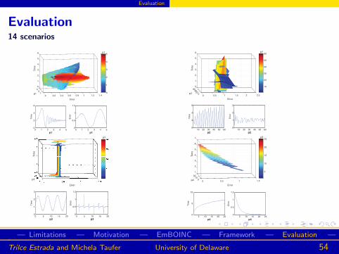
Evaluation14 scenarios

0 0.2 0.4 0.6 0.8 1 1.2 1.41

35

0

1

2

3

4

5

6

0

1

2

3

4

5

Tim

e

Error

p1

p1

0 1 2 3 4 50

2

4

6

Tim

e

p10 1 2 3 4 5

0

0.5

1

1.5

Err

or

p1

Tim

e

Error

p3

p3

0 5 10 15 200

1

2

3

Tim

e

p30 5 10 15 20

0

0.5

1

1.5

Err

or

p3

0 0.5 1 1.5 2 2.50

2040

60

0

1

2

3

4

5

6

10

20

30

40

50

60

Tim

e

Error

p2

p2

10 20 30 40 50 600

2

4

6

Tim

e

p210 20 30 40 50 60

0

1

2

3

Err

or

p2

0 0.5 1 1.50

1020

1

2

3

4

5

6

7

5

10

15

20

25

5 10 15 20 250

5

10

Tim

e

p45 10 15 20 25

0

0.5

1

1.5

Err

or

p4

Tim

e

Error

p4

p4

— Limitations — Motivation — EmBOINC — Framework — Evaluation —..

Trilce Estrada and Michela Taufer University of Delaware 54

Evaluation

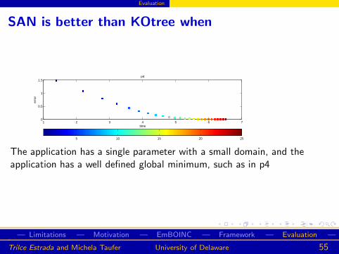
SAN is better than KOtree when

1 2 3 4 5 6 70

0.5

1

1.5

time

erro

r

p4

5 10 15 20 25

The application has a single parameter with a small domain, and theapplication has a well defined global minimum, such as in p4

— Limitations — Motivation — EmBOINC — Framework — Evaluation —..

Trilce Estrada and Michela Taufer University of Delaware 55

Evaluation

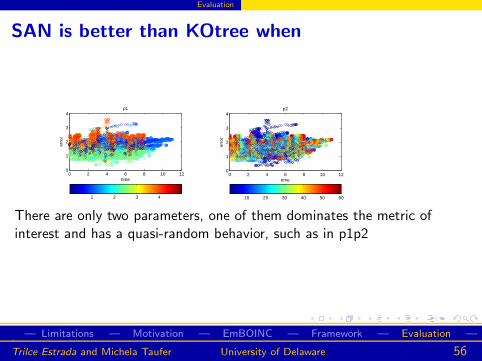
SAN is better than KOtree when

0 2 4 6 8 10 120

1

2

3

4

time

erro

r

p2

0 2 4 6 8 10 120

1

2

3

4

time

erro

r

p1

1 2 3 4 10 20 30 40 50 60

There are only two parameters, one of them dominates the metric ofinterest and has a quasi-random behavior, such as in p1p2

— Limitations — Motivation — EmBOINC — Framework — Evaluation —..

Trilce Estrada and Michela Taufer University of Delaware 56

Evaluation

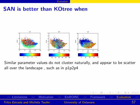
SAN is better than KOtree when

0 5 10 15 200

1

2

3

4

5

6

time

erro

r

p2

0 5 10 15 200

2

4

6

time

erro

r

p4

0 5 10 15 200

2

4

6

time

erro

r

p1

1 2 3 4 10 20 30 40 50 60 5 10 15 20 25

Similar parameter values do not cluster naturally, and appear to be scatterall over the landscape , such as in p1p2p4

— Limitations — Motivation — EmBOINC — Framework — Evaluation —..

Trilce Estrada and Michela Taufer University of Delaware 57

Evaluation

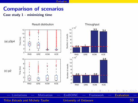
Comparison of scenariosCase study 1 - minimizing time

Smaller Similar Larger0

5

10

15

Nu

mb

er

of sce

na

rio

s

RND KOM KOE

57% 64%

0%

93%

Better Similar Worse

7% 7%14%

35%

21%

Better Similar Worse

KS test with respect to GREKolmorgorov-Smirnov test with respect to GRE

KOM is better than SAN in 57% of the cases and increasesthroughput in average 75%.

KOE is better than SAN in 64% of the cases and increasesthroughput in average 132%.

— Limitations — Motivation — EmBOINC — Framework — Evaluation —..

Trilce Estrada and Michela Taufer University of Delaware 58

Evaluation

Comparison of scenariosCase study 1 - minimizing time

RND GRE KOM KOE0

2

4

6

8

10

12

14x 10

4

Nu

mb

er

of re

su

lts

0.8 1

3.5 3.4

0.8 1

3.5 3.4

RND GRE KOM KOE0

2

4

6

8

10

12

14x 10

4

Nu

mb

er

of re

su

lts

0.9 1 0.9

2.8

0.9 1 0.9

2.8

RND GRE KOM KOE0

2

4

6

8

10

12

Tim

e (

hrs

)

RND GRE KOM KOE0

2

4

6

8

10

Tim

e (

hrs

)

Result distrbution Throughput

(a) p3p4

(c) p2

— Limitations — Motivation — EmBOINC — Framework — Evaluation —..

Trilce Estrada and Michela Taufer University of Delaware 59

Evaluation

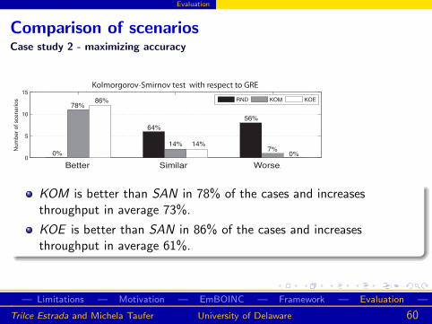
Comparison of scenariosCase study 2 - maximizing accuracy

Smaller Similar Larger0

5

10

15

Nu

mb

er

of sce

na

rio

s

KS test with respect to GRE

RND KOM KOE

Better Similar Worse

0% 0%

64%

56%

78%86%

7%14% 14%

Better Similar Worse

KS test with respect to GREKolmorgorov-Smirnov test with respect to GRE

KOM is better than SAN in 78% of the cases and increasesthroughput in average 73%.

KOE is better than SAN in 86% of the cases and increasesthroughput in average 61%.

— Limitations — Motivation — EmBOINC — Framework — Evaluation —..

Trilce Estrada and Michela Taufer University of Delaware 60

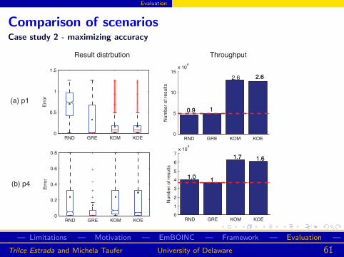
Evaluation

Comparison of scenariosCase study 2 - maximizing accuracy

RND GRE KOM KOE0

5

10

15x 10

4

Nu

mb

er

of re

su

lts

0.9 1

2.6 2.6

0.9 1

2.6

RND GRE KOM KOE0

1

2

3

4

5

6

7x 10

4

Nu

mb

er

of re

su

lts

1.01

1.7 1.6

1.01

1.7 1.6

RND GRE KOM KOE0

0.5

1

1.5

Err

or

RND GRE KOM KOE0

0.2

0.4

0.6

0.8

Err

or

Result distrbution Throughput

(a) p1

(b) p4

— Limitations — Motivation — EmBOINC — Framework — Evaluation —..

Trilce Estrada and Michela Taufer University of Delaware 61

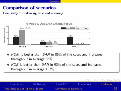
Evaluation

Comparison of scenariosCase study 3 - balancing time and accuracy

Smaller Similar Larger0

5

10

15

Nu

mb

er

of sce

na

rio

s

KS test with respect to GRE

RND KOM KOE

0% 0%7%

14% 14%

43% 43%

86%93%

Better Similar Worse

KS test with respect to GREKolmorgorov-Smirnov test with respect to GRE

KOM is better than SAN in 86% of the cases and increasesthroughput in average 85%.

KOE is better than SAN in 93% of the cases and increasesthroughput in average 107%.

— Limitations — Motivation — EmBOINC — Framework — Evaluation —..

Trilce Estrada and Michela Taufer University of Delaware 62

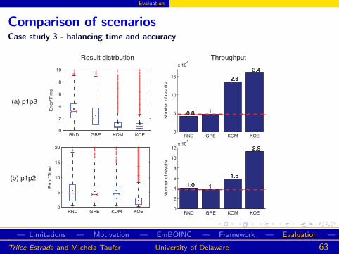
Evaluation

Comparison of scenariosCase study 3 - balancing time and accuracy

RND GRE KOM KOE0

5

10

15

x 104

Nu

mb

er

of re

su

lts

0.8 1

2.8

3.4

0.8 1

2.8

3.4

RND GRE KOM KOE0

2

4

6

8

10

12x 10

4

Nu

mb

er

of re

su

lts

1.0 1

1.5

2.9

1.0 1

1.5

2.9

RND GRE KOM KOE0

2

4

6

8

10

Err

or*

Tim

e

RND GRE KOM KOE0

5

10

15

20

Err

or*

Tim

e

Result distrbution Throughput

(a) p1p3

(b) p1p2

— Limitations — Motivation — EmBOINC — Framework — Evaluation —..

Trilce Estrada and Michela Taufer University of Delaware 63