on the effectiveness of phase based regression models to trade power and performance using dynamic...

Available online at www.sciencedirect.com

www.elsevier.com/locate/sysarc

Journal of Systems Architecture 54 (2008) 797–815

On the effectiveness of phase based regression models to tradepower and performance using dynamic processor adaptation

Subhasis Banerjee *, G. Surendra, S.K. Nandy

CAD Lab, Supercomputer Education and Research Centre, Indian Institute of Science, Bangalore 560 012, Karnataka, India

Received 23 September 2006; received in revised form 4 January 2008; accepted 15 February 2008Available online 4 March 2008

Abstract

Microarchitecture optimizations, in general, exploit the gross program behavior for performance improvement. Programs may beviewed as consisting of different ‘‘phases” which are characterized by variation in a number of processor performance metrics. Previousstudies have shown that many of the performance metrics remain nearly constant within a ‘‘phase”. Thus, the change in program‘‘phases” may be identified by observing the change in the values of these metrics. This paper aims to exploit the time varying behaviorof programs for processor adaptation. Since the resource usage is not uniform across all program ‘‘phases”, the processor operates atvarying levels of underutilization. During phases of low available Instruction Level Parallelism (ILP), resources may not be fully utilizedwhile in other phases, more resources may be required to exploit all the available ILP. Thus, dynamically scaling the resources based onprogram behavior is an attractive mechanism for power–performance trade-off. In this paper we develop per-phase regression models toexploit the phase behavior of programs and adequately allocate resources for a target power–performance trade-off. Modeling processorperformance–power using such a regression model is an efficient method to evaluate an architectural optimization quickly and accu-rately. We also show that the per-phase regression model is better suited than an ‘‘unified” regression model that does not use phaseinformation. Further, we describe a methodology to allocate processor resources dynamically by using regression models which aredeveloped at runtime. Our simulation results indicate that average energy savings of 20% can be achieved with respect to a maximallyconfigured system with negligible impact on performance for most of the SPEC-CPU and MEDIA benchmarks.� 2008 Elsevier B.V. All rights reserved.

Keywords: Processor microarchitecture; Program phases; Regression model

1. Introduction

The ‘‘phase” of an executing program can be viewed asthe window of the execution time during which the values ofobservable performance metrics remain almost constant.The performance metrics, when observed over the entireexecution of the program, exhibit periodicity and regular-ity. Therefore, one can conclude that programs ‘‘pass”

through different phases of execution. Though the execu-tion phase is not easily quantifiable, one can still obtainan overall estimation of the pattern of program executionbehavior from a plot of performance metrics. One such

1383-7621/$ - see front matter � 2008 Elsevier B.V. All rights reserved.

doi:10.1016/j.sysarc.2008.02.003

* Corresponding author.E-mail address: [email protected] (S. Banerjee).

plot is shown in Fig. 1. The plot shows the variation ininstruction per cycle (IPC), L-1 data cache miss rate andnormalized power dissipation for every five million instruc-tions for gcc benchmark. It is interesting to note thatthough the performance–power metrics do not change inthe same fashion, the transition in values of individual met-rics is almost always in synchronization with each other[14]. In other words, it is sufficient to track any of the con-venient metric and characterize the whole program in termsof it. IPC is one such convenient metric that can be used tocharacterize program execution phases.

Despite techniques such as voltage scaling and circuitlevel approaches to low power, power dissipation in highperformance microprocessors has steadily increased in everynew generation [6]. Therefore, it is important to evaluate

mailto:[email protected]

0 200 400 600 800 1000 12000

0.5

1

Nor

m. p

ower

0 200 400 600 800 1000 12000

5

10D

–L1

mis

s (%

)

0 200 400 600 800 1000 12000

2

4

IPC

Interval – – each point represents 5M instructions

Fig. 1. Variation of different processor metric at different interval.

798 S. Banerjee et al. / Journal of Systems Architecture 54 (2008) 797–815

power/energy consumption at different stages of the designand make important decisions early in the design process.This work takes a microarchitecture level approach toexplore the design space for power optimization. The advan-tage of a microarchitectural abstraction is that it can addressissues related to the application runtime behavior.

One way of realizing a power-aware architecture is byappropriately trading performance for power/energy bene-fit. This may be achieved by implementing an ‘‘adaptable”microarchitecture. An adaptable core is equipped withmodules that are scaled up/down to meet the targetpower–performance trade-off. The motivation for dynamicresource adaptation arises from the fact that a processorwith maximally configured resources does not always yieldhigh IPC across all execution phases of a program. Addi-tional energy spent in the maximum configuration is awaste when there is not enough potential to improve perfor-mance. Although the optimal conditions for performancemaximization (IPC maximization) and energy minimiza-tion are two conflicting goals, predefined trade-off objectivecan be met by scaling down resources with tolerable perfor-mance loss. Ideally, an adaptable architecture should emu-late the behavior of an oracle architecture which executesonly the useful instructions with optimally sized resources[33]. A well balanced runtime model of program executionbehavior can improve the adaptability of processor core forpower and performance optimization.

The main contributions of this paper are as follows:

(1) We classify the entire execution of a program into anumber of phases and fit piecewise linear regressionmodels for each execution phase. We then show thatthese per-phase regression models are better suited forestimating processor performance than a unified

regression model. Characterization of program exe-

cution phases is done in terms of average IPC overan ‘‘interval” of five million instructions. We demon-strate the working of the scheme using mpeg2decode

benchmark as a case study. Also, for the purpose ofcompleteness, we show results obtained for otherbenchmarks.

(2) We then show how these regression models can beused to allocate processor resources and trade someperformance for energy benefit. We use an ‘‘offline”profile analysis in which the complete informationof program phases is obtained from simulation runsand an optimal resource configuration is chosen tomeet a power–performance objective. In this stage,we assume that there is no penalty cycles incurredin ‘‘detecting” phases or in adapting (reconfiguring)processor parameters/resources. Therefore, theresults obtained indicate the limits of energy savingand performance loss with the given configuration.

(3) We propose a framework for runtime adaptation ofresources where performance counters sample differ-ent metrics in the processor core and collect necessarydata to generate regression models (at runtime). This‘‘online” scheme takes into account the penaltiesincurred during processor adaptation and assumesno prior knowledge of phases. Thus, phases are firstdynamically detected and then the processor parame-ters are appropriately configured to meet the targetpower–performance objective.

2. Related work

The behavior of a program was probably first analyzedusing a working set model by Denning [11]. The analysisand modeling of program behavior leads to a number of

Table 1Processor parameters used in the simulations

Parameter Value

LSQ size 32 InstructionsFetch/Decode/Issue/

Commit widthFour instructions/cycle

Branch predictor Combined predictor – bimodal 2K table, gshare1K table, 10 bit history1K chooser, 4 cycles penalty BTB – 2048 entry,4-way

Return address stack 16 entryL-1 data cache 64k 4-way, LRU, 32B block, 1 cycle latencyL-1 instruction cache 64K, 2-way, LRU, 32B block, 1 cycle latencyL-2 cache Unified, 1M, 4-way, LRU, 32B block, 15 cycle

latencyMemory 100 cycle first chunk latency, 2 cycles

subsequentlyTLB 128 entry itlb, 128 entry dtlb, 4-way, 30 cycle

miss latency

S. Banerjee et al. / Journal of Systems Architecture 54 (2008) 797–815 799

optimization policies that can be used to manage comput-ing resources effectively [10,27]. These computing resourcesare multiplexed among a number of ‘‘processes” or ‘‘activ-ities” of a computer program. From a programmer’s view-point, the working set is a collection of pages that arereferenced over a particular interval of time. A model torepresent the behavior of access pattern of pages helpsthe operating system to take appropriate decisions whileallocating different computing resources. The working setmodel using memory pages is not suitable for fine grainreconfiguration of the processor pipeline and cache mem-ory. Therefore, a closer observation of the processor execu-tion behavior at finer granularity (e.g., instruction workingset, basic block) is required. An approach to detect pro-gram phases by keeping track of the instruction workingset is explored in [13]. A basic block analysis to characterizeprogram behavior leads to a technique that identifies simu-lation points which represent gross program behavior [34].An extension of basic block behavior analysis to identifyprogram phases using dedicated hardware leads to trackingand predicting runtime behavior of a program [35]. Identi-fication of program phases along with the processor adap-tation policies lead to efficient management of resources forpower and performance optimization. Several adaptationmethods are proposed using temporal approach (whereprocessor adaptation is done in successive time slices[2,4]) as well as using positional approach (where the pro-cessor adaptation is done in code section of similar type[18]).

A number of power-aware microarchitectural optimiza-tions have been proposed to exploit program behavior. Forexample, reconfigurable caches have been used to minimizeenergy dissipation with tolerable performance loss [1,32]. Aresource scaling mechanism by searching the exhaustivedesign space of reconfigurable parameters is proposed in[19]. One limitation of such a technique is that with increas-ing design space, the overhead for reconfiguration increasesexponentially. In contrast, a regression model basedapproach certainly provides faster and more accuratereconfiguration.

There have been few attempts to develop superscalarprocessor models for faster performance evaluation[23,30]. Joseph et al. propose regression model to estimatethe performance of superscalar microprocessor [21,22]. Useof regression models to estimate performance as well aspower is proposed in [26]. All these work develop a unifiedmodel offline (not at runtime) to estimate performance–power for a given design point. In our work we constructregression models using runtime behavior of processor per-formance metrics, namely, IPC and energy dissipation.Further, the regression models are piecewise linear withinboundaries of distinguishable program phases. We developthe model using a subset of processor parameters that influ-ence IPC as well as energy most. First, we train the systemwith a set of simulation runs (training runs) and thendevelop a linear regression model for every distinguishableprogram phase. The methodologies proposed here include

both offline as well as runtime fitting of regression model.The power–performance trade-off achieved by using theselinear regression models leads to optimal design space con-figuration with better time complexity when compared withan exhaustive search technique.

3. Simulation environment

For our experiment we use a modified version of Wattch[7] which is based on SimpleScalar [8] – a cycle accurateexecution driven simulator. The built-in power model inWattch does not include static power dissipation. Weincorporate a number of modules from HotLeakage whichprovides a microarchitecture level model of sub-thresholdand gate leakage current [39]. In our simulation we use.13 lm process technology at 1.7 GHz clock frequency.Table 1 lists important SimpleScalar parameters that weuse in our simulation. These parameters closely resemblethe configuration of an Alpha 21264 processor core. Unlessotherwise mentioned, all simulations are carried out withthese parameter values.

In this work we use SPEC-CPU 2000 and MEDIAbenchmarks for our simulation. The benchmarks are simu-lated with MinneSPEC [24] inputs (for SPEC programs)and the large input data sets that were provided with theMiBench [17] distribution (in case of media programs).All the benchmarks are run to completion. To simulate arealistic processor platform, we use the SPEC Alpha bina-ries compiled for EV6 target architecture. The binaries arecompiled with �O3 level of optimization and are staticallylinked. For MEDIA benchmarks, we compiled the sourcecode using SimpleScalar gcc-2.6.3 for the PISA architecture[8]. The benchmarks that we use from SPEC-CPU are –bzip2, gzip, gcc, mcf, crafty, perlbmk, parser, vortex, twolf,applu, ammp, art, facerec, equake, mesa, galgel, swim andmgrid. MEDIA benchmarks that are used for our simula-tion are mpeg2 encode and decode (mpeg2encode, mpeg2de-

code), JPEG encode and decode (cjpeg, djpeg), mp3 audio


decode (lame) and adaptive differential PCM (pulse codemodulation) encoder and decoder (caudio, daudio).

4. Regression models to estimate performance and power

In order to devise appropriate regression models, wefirst need to understand the impact of various processorparameters on power and performance. For this purpose,we employ the Plackett–Burman [38] experimental design(P–B design) methodology which requires just 2ðN þ 1Þsimulations (with foldover [29]) to estimate the effect of N

parameters or factors. The P–B design is a non-geometrictwo level ‘‘fractional factorial” design [20] that is statisti-cally rigorous and can be used to determine the effects ofmain parameters and their interactions. This experimentenables designers to easily identify parameters that mustbe targeted by optimizations to obtain maximum benefits.It also indicates the influential parameters that must beconsidered in the design of future high performance andenergy efficient microprocessor architectures.

Based on the results of the P–B design, we observe thatthe instruction window (issue queue) size, number of Inte-ger ALU, number of floating point ALU, fetch width, L-1data and instruction cache latency, cache associativity andcache size predominantly influence the performance andenergy dissipation of a processor core. The effect of param-eters involved in cache design is faithfully reflected by thecache miss pattern at runtime. A study of L-1 data cachebehavior is presented in [5]. In [5], the authors proposeand evaluate a methodology to reconfigure L-1 data cacheat runtime using cache miss pattern. In this paper, the focusis on the front end parameters along with the functionalunits. The parameters are: instruction window size (issuequeue size), number of integer ALU, number of floatingpoint ALU and size of the fetch queue. These parametersare chosen since they are critical to the processor perfor-mance and also contribute significantly to the overallpower dissipation. For example, in the Alpha 21264 pro-cessor, the energy dissipated in the issue unit, IntegerALU and floating point ALU is 38% of the total energydissipated on chip [16]. To quantify the interactionsbetween parameters and the contribution of individualparameters, one needs to perform a ‘‘full factorial” [20]experiment (since the P–B design indicates only relativeimportance). We use a 2-level full factorial design with fourparameters that requires 24 or 16 simulations to constructthe regression models. As the number of training runs (sim-ulations) for developing the models using 2-level factorialdesign goes with power of 2 (2N, where N is number ofparameters), it is suitable for a design space with smallernumber of parameters. When the design space is large withmore number of parameters, A fractional factorial design(for example, P–B design) may be used to limit the numberof training run of the order of two times the number ofparameters considered. However, large design space willimpose significant overhead while constructing the regres-sion model at runtime.

In the following section we explain in detail the design ofthe full factorial experiment by considering mpeg2decode

benchmark as a case study. We also report importantresults for other benchmarks as well. Throughout the dis-cussion we use IPC and energy dissipation as the primarymetrics.

4.1. The 24 factorial design

The methodology involved in conducting a full factorialdesign experiment starts with choosing a set of parametersthat need to be evaluated and assigning them low and high

values. These low (denoted by ‘‘�”) and high (denoted by‘‘+”) values represent the two configuration limits (andhence denoted as 2-level design) of the parameters con-cerned. As mentioned previously, we use a four parameterfull factorial experiment with following low and high

values:

(1) Parameter A: Instruction window: 32 entry (�) and128 entry (+).

(2) Parameter B: Number of integer ALU: 2 (�) and 8(+).

(3) Parameter C: Number of floating point ALU: 1 (�)and 4 (+).

(4) Parameter D: Fetch queue: 4 entry (�) and 16 entry(+).

With four parameters, there are 16 possible experimentsthat can be conducted. Each such experiment is denotedby a sequence of at most four lower case letters. If a designparameter (say D) assumes a high value, it is represented byits lowercase (i.e., d). If a parameter assumes a low value, itis omitted from the sequence. The sequence of A, B, C andD is always maintained in order. For example, the combi-nation ‘abcd’ represents an experiment in which all param-eters have high values. Similarly, ‘abd’ represents anexperiment in which A = +, B = +, C = � and D = +.The combination with all low values is denoted by (1).The first column of Table 2 enlists all possible combinationfor a four parameter design space in the above mentionednotation.

For better understanding, we explain how the effects ofthe parameters are calculated for a two parameter full fac-torial design. Let A and B be the parameters under consid-eration. The effect of A is the average of the effectcomputed for both high and low values of B. Thus,EffA ¼ ab�bþa�ð1Þ

2. Here, ab is the value of the desired metric

for an experiment in which both A and B are high; a isvalue of the metric when A is high and B is low; (1) is thevalue of the metric when both A and B are low. In thisexpression, ðab� bÞ gives the effect of A when B is high

and ða� 1Þ gives the effect of A when B is low. A similarlogic is applicable for computing the effect ofB : EffB ¼ ab�aþb�ð1Þ

2. The effect of the interaction between

A and B, denoted by EffAB, is given by the average differ-ence between the effect of A at high level of B and effect

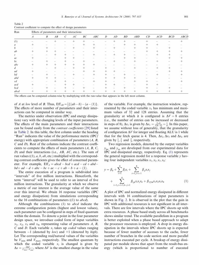
Table 2Contrast coefficient to compute the effect of design parameters

Run Effects of parameters and their interactions

A B AB C AC BC ABC D AD BD ABD CD ACD BCD ABCD

(1) – – + – + + – – + + – + – – +a + – – – – + + – – + + + + – –b – + – – + – + – + – + + – + –ab + + + – – – – – – – – + + + +c – – + + – – + – + + – – + + –ac + – – + + – – – – + + – – + +bc – + – + – + – – + – + – + – +abc + + + + + + + – – – – – – – –d – – + – + + – + – – + – + + –ad + – – – – + + + + – – – – + +bd – + – – + – + + – + – – + – +abd + + + – – – – + + + + – – – –cd – – + + – – + + – – + + – – +acd + – – + + – – + + – – + + – –bcd – + – + – + – + – + – + – + –abcd + + + + + + + + + + + + + + +

The effects can be computed column-wise by multiplying with the run-value that appears in the left most column.


of A at low level of B. Thus, EffAB¼ 12fðab�bÞ�ða�ð1Þg.

The effects of more number of parameters and their inter-actions can be computed in similar way.

The metrics under observation (IPC and energy dissipa-tion) vary with the changing levels of the input parameters.The effects of the main parameters and their interactionscan be found easily from the contrast coefficients [29] listedin Table 2. In this table, the first column under the heading‘‘Run” indicates the value of the performance metric (IPC/energy) with appropriate combination of parameters (A, B,C and D). Rest of the columns indicate the contrast coeffi-cients to compute the effects of main parameters (A, B, C,D) and their interactions (i.e., AB, AC, etc.). The sum ofrun values ((1), a, b, ab, etc.) multiplied with the correspond-ing contrast coefficients gives the effect of concerned param-eter. For example, EffA ¼ abcd � bcd þ acd � cd þ abd�bdþ ad � d þ abc� bcþ ac� cþ ab� bþ a� ð1Þ.

The entire execution of a program is subdivided into‘‘intervals” of five million instructions. Henceforth, theterm ‘‘interval” will be used to refer to an interval of fivemillion instructions. The granularity at which we observea metric of our interest is the average value of the sameover this interval. We obtain 16 response variables (IPCand energy dissipation) from simulations correspondingto the 16 combinations of parameters ((1) to abcd).

Although the combinations (1) to abcd indicate theextreme configuration points (highest and lowest values),each parameter can be configured in steps of fixed quantumwithin the domain. To denote a point in the four parameterdesign space, we introduce coded form of input variablesx1, x2, x3 and x4, representing value of parameters A, B,C and D. Each variable xi takes up coded values rangingbetween �1 (denoted by low) and +1 (denoted by high).Let The corresponding real/natural values of the variablesbe Vmin and Vmax, respectively. The smallest quantum bywhich the coded variable xi is changed is given byDx ¼ 2DV

V max�V min, where DV is the smallest change in the value

of the variable. For example, the instruction window, rep-resented by the coded variable x1 has minimum and maxi-mum values of 32 and 128 entries. Assuming that thegranularity at which it is configured is DV ¼ 8 entries(i.e., the number of entries can be increased or decreasedin steps of 8), Dx1 is given by Dx1 ¼ 2�8

128�32¼ 1

6. In this paper,

we assume without loss of generality, that the granularityof configuration DV for integer and floating ALU is 1 whilethat for the fetch queue is 4. Then, Dx2;Dx3 and Dx4 aregiven by 1

3; 2

3and 2

3, respectively.

Two regression models, denoted by the output variablesyipc and yen are developed from our experimental data forIPC and dissipated energy, respectively. Eq. (1) representsthe general regression model for a response variable y hav-ing four independent variables x1; x2; x3; x4:

y ¼ b0 þX4

i¼1

bixi þX4

i¼1;j¼iþ1

bijxixj

þX4

i¼1;j¼iþ1;k¼jþ1

bijkxixjxk þ b1234x1x2x3x4 ð1Þ

A plot of IPC and normalized energy dissipated in differentintervals with 16 combinations of input parameters isshown in Fig. 2. It is observed in the plot that the gain inIPC with additional resources is not significant in all inter-vals. There are few intervals where the IPC shoots up withextra resources. A phase based study across all benchmarksshows similar trend. The available parallelism in a programis better exploited when a phase based approach to adaptthe processor resources is employed. A drop in energy dis-sipation in the intervals where IPC shoots up is expectedbecause of fewer number of accesses to the cache, fewernumber of branches in the code section and more parallelinstructions executed per cycle. A breakup of energy dissi-pated per module shows that apart from the result-bus en-ergy (which is proportional to number of executed

0 10 20 30 40 50 60

2

2.5

3

3.5

Interval – – each point represents 5 million instruction

IPC

1ababcacbcabcdadbdabdcdacdbcdabcd

0 10 20 30 40 50 600.55

0.6

0.65

0.7

0.75

0.8

0.85

0.9

0.95

1

Interval – – each point represents 5 million instruction

Nor

mal

ized

ene

rgy

w.r

.t m

axim

um e

nerg

y di

ssip

ated

1ababcacbcabcdadbdabdcdacdbcdabcd

Fig. 2. IPC and energy variation in different execution intervals for mpeg2decode.


instructions), other energy components decrease in highIPC intervals.

Fig. 3 shows the absolute values of the effects of allparameters obtained in different intervals of execution forthe mpeg2decode benchmark. These results are obtainedby evaluating all combinations of parameters in everyinterval using the contrast coefficients of Table 2. Similarplots are obtained for all benchmarks to estimate the effectsof main parameters and their interactions. It is observedthat the effect of higher order interaction between parame-ters is small compared to individual parameters. Specifi-cally, the interaction between 2 or more parameters is

negligible. Therefore, the coefficients responsible for sec-ond, third and fourth order interaction are assumed to bezero, i.e., bij ¼ bijk ¼ b1234 ¼ 0. Thus, the regression equa-tions for IPC and energy reduce to the linear form asdescribed in following equation

yipc ¼ b0 þ b1x1 þ b2x2 þ b3x3 þ b4x4

yen ¼ a0 þ a1x1 þ a2x2 þ a3x3 þ a4x4

ð2Þ

In matrix representation, the equations can be written as

yipc ¼ Xb

yen ¼ Xað3Þ

A B AB C AC BC ABC D AD BD ABD CD ACD BCD ABCD0

1

2

3

4

5

6

7

8

9

10

Parameter combination

Rel

ativ

e ef

fect

on

IPC

A B AB C AC BC ABC D AD BD ABD CD ACD BCD ABCD0

0.2

0.4

0.6

0.8

1

1.2

1.4

1.6

1.8

2

Parameter combination

Rel

ativ

e ef

fect

on

ener

gy

Fig. 3. Effect of parameters on IPC and energy.


where yipc and yen are column vectors obtained from 16 runswith the coded variables and X is the matrix formed by thesecoded variables. The first column of X corresponds to theintercept terms of the regression equation. Therefore, it is acolumn vector containing all 1. Columns 2–5 contain thecoded values of variables x1; x2; x3 and x4. The solutions forb and a for the regression equations (3) are given in followingequation

b ¼ ðXTXÞ�1XTyipc

a ¼ ðXTXÞ�1XTyen

ð4Þ

4.2. Identification of program execution phases

The IPC recorded within an interval quantifies the avail-able ILP in the program in that interval. During the profile

run of a program we obtain the IPC variation for all con-figurations of the four configurable resources mentionedearlier. An analysis of IPC values with different configura-tion indicates that with higher configuration the variationin IPC is distinct from one phase to another. Although,in lower configuration the transition points between phasesremain the same, we use the maximum configuration todetect phase changes in our offline phase detection mecha-nism. To identify regions of different ILP, we classify eachinterval into different IPC domains. Each IPC domain isclassified as an unique execution phase. We detect phasechange from one interval to another by a masking opera-tion. A simple mask of five elements [�1, �1, 0, 1, 1] witha ‘‘sliding window” multiply–add operation on every inter-val of the IPC profile is used in our algorithm. While there

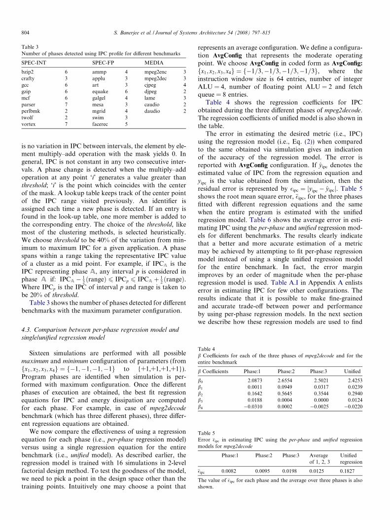
Table 3Number of phases detected using IPC profile for different benchmarks

SPEC-INT SPEC-FP MEDIA

bzip2 6 ammp 4 mpeg2enc 3crafty 3 applu 3 mpeg2dec 3gcc 6 art 3 cjpeg 4gzip 6 equake 6 djpeg 2mcf 6 galgel 4 lame 3parser 7 mesa 3 caudio 2perlbmk 2 mgrid 4 daudio 2twolf 2 swim 3vortex 7 facerec 5


is no variation in IPC between intervals, the element by ele-ment multiply–add operation with the mask yields 0. Ingeneral, IPC is not constant in any two consecutive inter-vals. A phase change is detected when the multiply–addoperation at any point ‘i’ generates a value greater thanthreshold; ‘i’ is the point which coincides with the centerof the mask. A lookup table keeps track of the center pointof the IPC range visited previously. An identifier isassigned each time a new phase is detected. If an entry isfound in the look-up table, one more member is added tothe corresponding entry. The choice of the threshold, likemost of the clustering methods, is selected heuristically.We choose threshold to be 40% of the variation from min-imum to maximum IPC for a given application. A phasespans within a range taking the representative IPC valueof a cluster as a mid point. For example, if IPCA is theIPC representing phase A, any interval p is considered inphase A if: IPCA � 1

2ðrangeÞ 6 IPCp 6 IPCA þ 1

2ðrangeÞ.

Where IPCp is the IPC of interval p and range is taken tobe 20% of threshold.

Table 3 shows the number of phases detected for differentbenchmarks with the maximum parameter configuration.

Table 4b Coefficients for each of the three phases of mpeg2decode and for theentire benchmark

b Coefficients Phase:1 Phase:2 Phase:3 Unified

b0 2.0873 2.6554 2.5021 2.4253b1 0.0011 0.0949 0.0317 0.0239b2 0.1642 0.5645 0.3544 0.2940b3 0.0188 0.0004 0.0000 0.0124b4 �0.0310 0.0002 �0.0025 �0.0220

Table 5Error ��ipc in estimating IPC using the per-phase and unified regressionmodels for mpeg2decode

Phase:1 Phase:2 Phase:3 Averageof 1, 2, 3

Unifiedregression

��ipc 0.0082 0.0095 0.0198 0.0125 0.1827

The value of ��ipc for each phase and the average over three phases is alsoshown.

4.3. Comparison between per-phase regression model and

single/unified regression model

Sixteen simulations are performed with all possiblemaximum and minimum configuration of parameters (fromfx1; x2; x3; x4g ¼ f�1;�1;�1;�1g to {+1,+1,+1,+1}).Program phases are identified when simulation is per-formed with maximum configuration. Once the differentphases of execution are obtained, the best fit regressionequations for IPC and energy dissipation are computedfor each phase. For example, in case of mpeg2decodebenchmark (which has three different phases), three differ-ent regression equations are obtained.

We now compare the effectiveness of using a regressionequation for each phase (i.e., per-phase regression model)versus using a single regression equation for the entirebenchmark (i.e., unified model). As described earlier, theregression model is trained with 16 simulations in 2-levelfactorial design method. To test the goodness of the model,we need to pick a point in the design space other than thetraining points. Intuitively one may choose a point that

represents an average configuration. We define a configura-tion AvgConfig that represents the moderate operatingpoint. We choose AvgConfig in coded form as AvgConfig:

fx1; x2; x3; x4g ¼ f�1=3;�1=3;�1=3;�1=3g, where theinstruction window size is 64 entries, number of integerALU = 4, number of floating point ALU = 2 and fetchqueue = 8 entries.

Table 4 shows the regression coefficients for IPCobtained during the three different phases of mpeg2decode.The regression coefficients of unified model is also shown inthe table.

The error in estimating the desired metric (i.e., IPC)using the regression model (i.e., Eq. (2)) when comparedto the same obtained via simulation gives an indicationof the accuracy of the regression model. The error isreported with AvgConfig configuration. If yipc denotes theestimated value of IPC from the regression equation andyipc is the value obtained from the simulation, then theresidual error is represented by �ipc ¼ jy ipc � yipcj. Table 5shows the root mean square error, ��ipc, for the three phasesfitted with different regression equations and the samewhen the entire program is estimated with the unifiedregression model. Table 6 shows the average error in esti-mating IPC using the per-phase and unified regression mod-els for different benchmarks. The results clearly indicatethat a better and more accurate estimation of a metricmay be achieved by attempting to fit per-phase regressionmodel instead of using a single unified regression modelfor the entire benchmark. In fact, the error marginimproves by an order of magnitude when the per-phaseregression model is used. Table A.I in Appendix A enlistserror in estimating IPC for few other configurations. Theresults indicate that it is possible to make fine-grainedand accurate trade-off between power and performanceby using per-phase regression models. In the next sectionwe describe how these regression models are used to find

Table 6Error in estimating IPC using per-phase and unified regression models for AvgConfig


Per-phase Unified Per-phase Unified Per-phase Unified

bzip2 0.0012 0.4472 ammp 0.0027 0.4098 mpeg2enc 0.0086 0.5059crafty 0.0013 0.6556 applu 0.0027 0.0706 mpeg2dec 0.0125 0.1827gcc 0.0045 0.3519 art 0.0131 0.8762 cjpeg 0.0065 0.2359gzip 0.0031 0.4632 equake 0.0059 0.6270 djpeg 0.0005 0.1632mcf 0.0014 0.6263 galgel 0.0089 0.4521 lame 0.0045 0.0656parser 0.0161 0.8923 mesa 0.0039 0.5021 caudio 0.0031 0.2512perlbmk 0.0025 0.5239 mgrid 0.0102 0.7809 daudio 0.0016 0.1391twolf 0.0022 0.5612 swim 0.0086 0.5622vortex 0.0131 0.4591 facerec 0.0078 0.3102


optimal configuration of design parameters to achieve atarget power–performance trade-off.

5. Obtaining the optimal configuration from regression

models

Once we obtain per-phase regression equations for IPCand energy, we are in a position to formally state the opti-mization problem. Our goal is now to find the appropriatecombination of the design parameters for which the mini-mization of energy is achieved by limiting the IPC loss.The optimization problem that we attempt to solve canbe stated as follows:

minimize : yen ¼X4

i¼1

aixi

subject to :X4

i¼1

bixi P k

x1 2 �1;� 5

6;� 4

6; . . . ;

4

6;5

6;þ1

� �

x2 2 �1;� 2

3;� 1

3; 0;

1

3;2

3;þ1

� �

x3 2 �1;� 1

3;1

3;þ1

� �

x4 2 �1;� 1

3;1

3;þ1

� �

ð5Þ

We assume that our baseline configuration is a maximallyconfigured machine where all the parameters are set to+1 ðfx1; x2; x3; x4g ¼ fþ1;þ1;þ1;þ1gÞ. We minimize theenergy yen by limiting the performance loss to a predefinedlimit. In the present case we assume the maximum perfor-mance (IPC) loss is 2% of that of a maximally configuredsystem. Therefore, in Eq. (5), k is a constant which is givenby k ¼ 0:98ymax

ipc � b0 � ymaxipc is the IPC with maximum con-

figuration. It must be noted that each coded parameter xi ischanged in discrete steps of Dxi. Thus, xi takes discrete val-

ues as shown in Eq. (5). The term a0 is a constant andtherefore is omitted from the energy equation.

Since the maximization of y ipc and minimization of yen

are two conflicting optimization goals, the simultaneoussolution to these equations is not possible. We thereforeminimize yen by imposing a lower bound on yipc. Table 7shows the regression coefficients for yipc and yen along withxi as appropriate for maximizing IPC and minimizingenergy (for mpeg2decode) without imposing any boundon them. The table also shows the energy saving and corre-sponding performance loss using min:Energy configurationwhen compared with the maximally configured system(maxConfig:{xi} = {+1, +1, +1, +1}). It is observed thatin phase:1, min:Energy configuration results in 31.8%energy saving with 13.7% loss in IPC. At the same timeother two phases show loss of 5.7% and 2.2% IPC whilesaving 29.4% and 28.2% energy, respectively. This exampleshows that we need to limit the performance loss in allthree phases of program execution so that the overallIPC is not compromised beyond the tolerable limit (2%in the present case). By setting the configuration of theresources appropriately such trade-off points can beachieved from the regression models developed in each exe-cution phase.

It is found that in each phase, some parameters remainunchanged for maximum IPC and minimum energy config-uration. For example, in Table 7, x4 remains unchanged(and has a value �1) for both max:IPC and min:Energy.Similarly, x2 and x4 remain unchanged in phase:2 andx2 and x3 remain unchanged in phase:3. One favorableaspect of parameters remaining unchanged is that thesearch space to obtain a suitable power–performancetrade-off point reduces.

Table 7 provides another interesting observation that iscounter intuitive. It indicates that for minimum energy dis-sipation, the processor parameters need not always assumeminimal or low (or �1) values. For example, in phase:2 andphase:3, min:Energy is achieved with the maximum config-uration of x2 (i.e., number of integer ALU = 8) and x4 (i.e.,fetch queue size = 16 entries). This is confirmed by the plotin Fig. 4. In the regions of high ILP, more functional unitsand wider fetch queue help faster completion of instruc-tions in the pipeline. The memory accesses are few in these

0 10 20 30 40 50 600.56

0.58

0.6

0.62

0.64

0.66

0.68

0.7

0.72

0.74

Interval

Nor

mal

ized

ene

rgy

1(–1,–1,–1,–1)bd(–1,1,–1,1)

Fig. 4. Normalized energy dissipation in different execution phases for mpeg2decode for (1) and bd configuration.

Table 7The optimal parameter values and corresponding b and a coefficients for (i) maximization of IPC with no energy constraint (denoted by max:IPC) and (ii)minimization of energy with no performance constraint (denoted by min:Energy) for the three phases in mpeg2decode

Phase:1 Phase:2 Phase:3

max:IPC min:Energy max:IPC min:Energy max:IPC min:Energy

bi xi ai xi bi xi ai xi bi xi ai xi

2.0873 1 0.8347 1 2.6554 1 0.7309 1 2.5021 1 0.8000 10.0011 1 0.1114 �1 0.0949 1 0.0800 �1 0.0317 1 0.0876 �10.1642 1 0.0084 �1 0.5645 1 �0.0467 1 0.3544 1 �0.0232 10.0188 1 0.0312 �1 0.0004 1 0.0377 �1 0.0000 �1 0.0397 �1�0.0310 �1 0.0067 �1 0.0002 1 �0.0013 1 �0.0025 �1 �0.0001 1

% Energy saving/ % IPC loss

31.8/13.7 29.4/5.7 28.2/2.2

Energy saving and IPC loss are computed with respect to maximally configured system i.e., {+1, +1, +1, +1}.


regions and that results in lower energy dissipation. Low

values of x2 and x4 in these regions result in higher powerin these intervals as instructions tend to remain longer inthe pipeline.

To arrive at the optimal operating point that satisfies thepredefined trade-off stated in Eq. (5) we use IPC and energyregression models. We use a linear programming solver1 toobtain the required combination. As xi take discrete values,the nearest point in the feasible set is chosen as the solutionfor x. For mpeg2decode the optimal solution in threephases are as follows:

� Phase:1 fxig ¼ f�1; 12;�1;�1g; energy saving = 30.5%,

IPC loss = 2.7%.� Phase:2 fxig ¼ f1

3; 1;�1; 1g; energy saving = 16.1%, IPC

loss = 1.9%.

1 linprog function in MATLAB [28].

� Phase:3 fxig ¼ f�1; 1;�1;�1g; energy saving = 28.1%,IPC loss = 2.0%.

It must be noted that the IPC loss crosses the limit of 2%in some execution phases. This is due to the fact that the dis-crete value of xi (in the feasible set described in Eq. (5))takes a lower configuration point than the one obtainedusing linear programming solver. Results indicate that eachphase requires a different resource configuration to achievethe desired power–performance trade-off. It also provides ajustification for the use of per-phase regression modelsinstead of using a unified model for the entire benchmark.It must be noted that the optimal set of parameters can takeany value from the set of all possible values for the respec-tive parameters mentioned in Eq. (5). b; a and the optimalconfiguration of parameters along with ‘‘Energy saving”and ‘‘IPC loss” for few benchmarks are listed in TablesA.II, A.III and A.IV, respectively (in Appendix A).


5.1. Simulation results

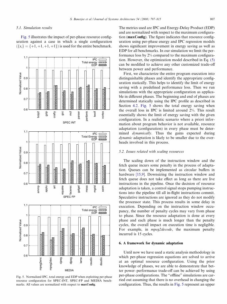
Fig. 5 illustrates the impact of per-phase resource config-uration against a case in which a single configurationðfxig ¼ fþ1;þ1;þ1;þ1gÞ is used for the entire benchmark.

0.6

0.7

0.8

0.9

1

1.1

vort

ex

twol

f

perlb

mk

pars

er

mcf

gcc

craf

ty

gzip

bzip

2

Nor

mal

ized

Val

ue

SPEC INT

IPCTotal energy

EDP

0.6

0.7

0.8

0.9

1

1.1

swim

mgr

id

mes

a

galg

el

face

rec

equa

keart

appl

u

amm

p

Nor

mal

ized

Val

ue

SPEC FP

IPCTotal Energy

EDP

0.6

0.7

0.8

0.9

1

1.1

daud

io

caud

io

lam

e

djpe

g

cjpe

g

mpe

g2de

c

mpe

g2en

c

Nor

mal

ized

Val

ue

MEDIA

IPCTotal energy

EDP

Fig. 5. Normalized IPC, total energy and EDP when exploiting per-phaseresource configuration for SPEC-INT, SPEC-FP and MEDIA bench-marks. All values are normalized with respect to maxConfig.

The metrics used are IPC and Energy-Delay Product (EDP)and are normalized with respect to the maximum configura-tion (maxConfig). The figure indicates that resource config-uration using per-phase energy and IPC regression modelsshows significant improvement in energy saving as well asEDP for all benchmarks. In our simulation we limit the per-formance loss by 2% compared to the maximum configura-tion. However, the optimization model described in Eq. (5)can be modified to achieve any other customized trade-offbetween power and performance.

First, we characterize the entire program execution intodistinguishable phases and identify the appropriate config-uration statically. This helps to identify the limit of energysaving with a predefined performance loss. Then we runsimulations with the appropriate configuration as applica-ble in different phases. The beginning and end of phases aredetermined statically using the IPC profile as described inSection 4.2. Fig. 5 shows the total energy saving whenthe overall loss in IPC is limited around 2%. This resultessentially shows the limit of energy saving with the givenconfiguration. In a realistic scenario where a priori infor-mation about program behavior is not available, resourceadaptation (configuration) in every phase must be deter-mined dynamically. Thus the gains expected duringdynamic adaptation is likely to be smaller due to the over-heads involved in this process.

5.2. Issues related with scaling resources

The scaling down of the instruction window and thefetch queue incurs some penalty in the process of adapta-tion. Queues can be implemented as circular buffers inhardware [15,9]. Downsizing the instruction window andfetch queue does not take effect as long as there are liveinstructions in the pipeline. Once the decision of resourceadaptation is taken, a control signal stops pumping instruc-tions into the pipeline till all in-flight instructions commit.Speculative instructions are ignored as they do not modifythe processor state. This process results in some delay inexecution. Depending on the instruction window occu-pancy, the number of penalty cycles may vary from phaseto phase. Since the resource adaptation is done at everyphase and each phase is much longer than the penaltycycles, the overall impact on execution time is negligible.For example, in mpeg2decode, the maximum penaltyincurred is 15 cycles.

6. A framework for dynamic adaptation

Until now we have used a static analysis methodology inwhich per-phase regression equations are solved to arriveat an optimal resource configuration. Using the priorknowledge of phases, we are able to demonstrate that bet-ter power–performance trade-off can be achieved by usingper-phase configurations. The ‘‘offline” simulations are car-ried out assuming that there is no overhead in changing theconfiguration. Thus, the results in Fig. 5 represent an upper


bound. For the rest of the paper we focus our attention ondynamic adaptation of processor resources based on theprogram phase information. In the dynamic adaptationscheme the regression models for IPC as well as energyare developed at runtime for every new phase (or in a pre-viously determined phase where error in estimating IPC/energy exceeds a threshold). We incorporate additionalpenalty cycles to account for dynamic adaptation therebyensuring that the simulations are as close to reality aspossible.

6.1. Instruction energy estimation

A study of the power dissipated by individual instructionis investigated by an experimental setup in [36]. The authorsuse a direct power measurement technique by probing into

0

1

2

3

4

5

6

7

8

Reg

file

Inst

Win

dow

Int-

ALU

Fp-

ALU

L1-I

cac

he

L1-D

cahe

L2-U

cac

he

Nor

mal

ized

ene

rgy

(w.r

.t re

gfile

ene

rgy)

Fig. 6. Energy dissipated in different modules normalized to the register-file energy.

FE

TC

H

INTALU

CONTROL REG

ISS

UE

Q

ALUFP

REG

COUNTERS

PERFORMANCE

CTRL WORDID

CONTROLTABLE

DETECTOR

PHASE

P

SELECT

ProcessorCore

Fig. 7. A framework for

the processor hardware setup. In our experiment we use oursimulator to estimate dissipated power for a class of instruc-tion by running a number of test kernels that are written inAlpha assembly instructions supported by the simulator.The test kernels contain a particular group of instructions(for example: integer, floating point, load/store instruc-tions) and are executed in a loop several times before thefinal statistic is collected. Fig. 6 shows the relative energydissipation per access to the individual modules normalizedwith respect to the register file energy. We use these num-bers to devise a look-up table based power counter thatcan provide an estimate of the relative energy dissipationwhile running a program. Such performance counters canbe easily built into the processor hardware.

6.2. Working details

Since the instruction window is the most power consum-ing unit, it has received much attention in literature. Someschemes for reconfiguring the instruction window havebeen explored in [3,9,31]. These schemes are essentiallybased on enabling or disabling portions of the queues usingcontrol signals (e.g., clock gating). As mentioned previ-ously, in our simulations the instruction window and thefetch queue are configured at a granularity of 8 and 4entries, respectively. The integer and floating point ALUare configured by powering on/off each individual unit(granularity of 1). All the modules are assumed to be clockgated when not operational. A control signal enables theseunits on demand basis.

We propose a framework to implement dynamic powermanagement to achieve a target power–performance trade-off by using hardware support. Fig. 7 shows the schematicdiagram of the framework. The look-up table in the figure

CONTROL

POWER CTR

TABLELOOK UP

REDICTOR

PHASE

+

FromProcessorCore

dynamic adaptation.


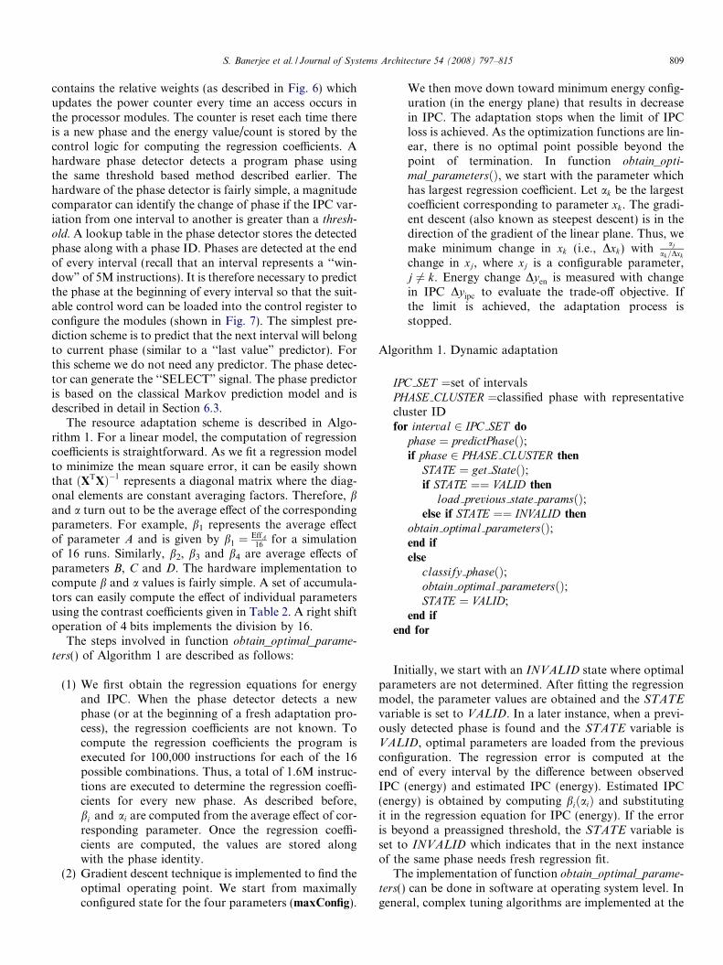
contains the relative weights (as described in Fig. 6) whichupdates the power counter every time an access occurs inthe processor modules. The counter is reset each time thereis a new phase and the energy value/count is stored by thecontrol logic for computing the regression coefficients. Ahardware phase detector detects a program phase usingthe same threshold based method described earlier. Thehardware of the phase detector is fairly simple, a magnitudecomparator can identify the change of phase if the IPC var-iation from one interval to another is greater than a thresh-

old. A lookup table in the phase detector stores the detectedphase along with a phase ID. Phases are detected at the endof every interval (recall that an interval represents a ‘‘win-dow” of 5M instructions). It is therefore necessary to predictthe phase at the beginning of every interval so that the suit-able control word can be loaded into the control register toconfigure the modules (shown in Fig. 7). The simplest pre-diction scheme is to predict that the next interval will belongto current phase (similar to a ‘‘last value” predictor). Forthis scheme we do not need any predictor. The phase detec-tor can generate the ‘‘SELECT” signal. The phase predictoris based on the classical Markov prediction model and isdescribed in detail in Section 6.3.

The resource adaptation scheme is described in Algo-rithm 1. For a linear model, the computation of regressioncoefficients is straightforward. As we fit a regression modelto minimize the mean square error, it can be easily shownthat ðXTXÞ�1 represents a diagonal matrix where the diag-onal elements are constant averaging factors. Therefore, band a turn out to be the average effect of the correspondingparameters. For example, b1 represents the average effectof parameter A and is given by b1 ¼ EffA

16for a simulation

of 16 runs. Similarly, b2, b3 and b4 are average effects ofparameters B, C and D. The hardware implementation tocompute b and a values is fairly simple. A set of accumula-tors can easily compute the effect of individual parametersusing the contrast coefficients given in Table 2. A right shiftoperation of 4 bits implements the division by 16.

The steps involved in function obtain_optimal_parame-

ters() of Algorithm 1 are described as follows:

(1) We first obtain the regression equations for energyand IPC. When the phase detector detects a newphase (or at the beginning of a fresh adaptation pro-cess), the regression coefficients are not known. Tocompute the regression coefficients the program isexecuted for 100,000 instructions for each of the 16possible combinations. Thus, a total of 1.6M instruc-tions are executed to determine the regression coeffi-cients for every new phase. As described before,bi and ai are computed from the average effect of cor-responding parameter. Once the regression coeffi-cients are computed, the values are stored alongwith the phase identity.

(2) Gradient descent technique is implemented to find theoptimal operating point. We start from maximallyconfigured state for the four parameters (maxConfig).

We then move down toward minimum energy config-uration (in the energy plane) that results in decreasein IPC. The adaptation stops when the limit of IPCloss is achieved. As the optimization functions are lin-ear, there is no optimal point possible beyond thepoint of termination. In function obtain_opti-mal_parametersðÞ, we start with the parameter whichhas largest regression coefficient. Let ak be the largestcoefficient corresponding to parameter xk. The gradi-ent descent (also known as steepest descent) is in thedirection of the gradient of the linear plane. Thus, wemake minimum change in xk (i.e., Dxk) with

aj

ak=Dxk

change in xj, where xj is a configurable parameter,j 6¼ k. Energy change Dyen is measured with changein IPC Dyipc to evaluate the trade-off objective. Ifthe limit is achieved, the adaptation process isstopped.

Algorithm 1. Dynamic adaptation

IPC SET ¼set of intervalsPHASE CLUSTER ¼classified phase with representativecluster IDfor interval 2 IPC SET do

phase ¼ predictPhaseðÞ;if phase 2 PHASE CLUSTER then

STATE ¼ get StateðÞ;if STATE ¼¼ VALID then

load previous state paramsðÞ;else if STATE ¼¼ INVALID then

obtain optimal parametersðÞ;end if

else

classify phaseðÞ;obtain optimal parametersðÞ;STATE ¼ VALID;

end if

end for

Initially, we start with an INVALID state where optimalparameters are not determined. After fitting the regressionmodel, the parameter values are obtained and the STATE

variable is set to VALID. In a later instance, when a previ-ously detected phase is found and the STATE variable isVALID, optimal parameters are loaded from the previousconfiguration. The regression error is computed at theend of every interval by the difference between observedIPC (energy) and estimated IPC (energy). Estimated IPC(energy) is obtained by computing biðaiÞ and substitutingit in the regression equation for IPC (energy). If the erroris beyond a preassigned threshold, the STATE variable isset to INVALID which indicates that in the next instanceof the same phase needs fresh regression fit.

The implementation of function obtain_optimal_parame-ters() can be done in software at operating system level. Ingeneral, complex tuning algorithms are implemented at the


level of virtual machine abstraction or in operating system[12]. In our simulation we assume that the control compu-tations are done by the operating system with the help ofthe phase detector, performance counters and the powercounter. The control table contains phase identity detectedby the phase detector along with the control word to adaptthe processor core. The control word in the control table isupdated by the control algorithm. In our simulations we donot assume any delay due to computation involved indetermining the regression coefficients. However, we incor-porate delays due to resizing instruction window asdescribed in Section 5.2.

6.3. Prediction of program execution phases

Locality in program behavior indicates that once a pro-gram enters into an execution phase, it continues to be inthat phase for several intervals. A phase change is generallyassociated with abrupt change in an observable metric. Inthe dynamic scheme of adaptation, a given interval isassigned a phase identity at the end of the interval. A

Run length Next ID

Detector

PhaseRun Length

Encoder

Logic

Prediction

Predicted Phase

Update

Predictor table

Fig. 8. Schematic phase predictor.

5

10

15

20

25

30

appl

uam

mp

vort

extw

olf

perlb

mk

pars

erm

cfgc

ccr

afty

gzip

bzip

2

Per

cent

mis

pred

ictio

n

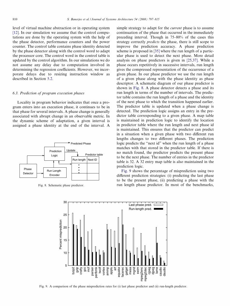
Fig. 9. A comparison of the phase misprediction rates for

simple strategy to adapt for the current phase is to assumecontinuation of the phase that occurred in the immediatelypreceding interval. Though in 75–80% of the cases thisstrategy correctly predicts the phase, there is still scope toimprove the prediction accuracy. A phase predictionscheme is proposed in [35] where the run length of a partic-ular phase is used to detect the next phase. More detailanalysis on phase predictors is given in [25,37]. While aphase occurs repetitively in successive intervals, run lengthgives the compressed representation of the occurrence of agiven phase. In our phase predictor we use the run lengthof a given phase along with the phase identity as phasedescriptor. A schematic diagram of our phase predictor isshown in Fig. 8. A phase detector detects a phase and itsrun length in terms of the number of intervals. The predic-tor table contains the run length of a phase and the identityof the next phase to which the transition happened earlier.The predictor table is updated when a phase change isdetected. The prediction logic assigns an entry in the pre-dictor table corresponding to a given phase. A map tableis maintained in prediction logic to identify the locationin predictor table where the run length and next phase idis maintained. This ensures that the predictor can predictin a situation when a given phase with two different runlengths changes to two different phases. The predictionlogic predicts the ‘‘next id” when the run length of a phasematches with that stored in the predictor table. If there isno match found, the predictor predicts the present phaseto be the next phase. The number of entries in the predictortable is 32. A 32 entry map table is also maintained in theprediction logic.

Fig. 9 shows the percentage of misprediction using twodifferent prediction strategies: (i) predicting the last phaseto be the present phase, (ii) predicting a phase with therun length phase predictor. In most of the benchmarks,

daud

ioca

udio

lam

edj

peg

cjpe

gm

peg2

dec

mpe

g2en

csw

imm

grid

mes

aga

lgel

face

rec

equa

keart

Last phase pred.Run-length pred.

(i) last phase predictor and (ii) run-length predictor.


the run-length prediction performs better than the lastphase prediction strategy. The misprediction rate for boththe schemes is nearly identical for benchmarks with

0.6

0.7

0.8

0.9

1

1.1

vort

ex

twol

f

perlb

mk

pars

er

mcf

gcc

craf

ty

gzip

bzip

2

Nor

mal

ized

Val

ue

SPEC INT

IPCTotal energy

EDP

0.6

0.7

0.8

0.9

1

1.1

swim

mgr

id

mes

a

galg

el

face

rec

equa

keart

appl

u

amm

p

Nor

mal

ized

Val

ue

SPEC FP

IPCTotal energy

EDP

0.6

0.7

0.8

0.9

1

1.1

daud

io

caud

io

lam

e

djpe

g

cjpe

g

mpe

g2de

c

mpe

g2en

c

Nor

mal

ized

Val

ue

MEDIA

IPCTotal Energy

EDP

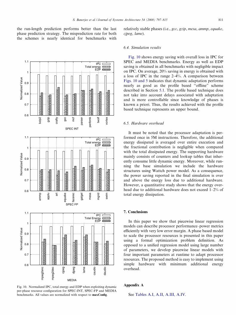
Fig. 10. Normalized IPC, total energy and EDP when exploiting dynamicper-phase resource configuration for SPEC-INT, SPEC-FP and MEDIAbenchmarks. All values are normalized with respect to maxConfig.

relatively stable phases (i.e., gcc, gzip, mesa, ammp, equake,cjpeg, lame).

6.4. Simulation results

Fig. 10 shows energy saving with overall loss in IPC forSPEC and MEDIA benchmarks. Energy as well as EDPsaving is obtained in all benchmarks with negligible impacton IPC. On average, 20% saving in energy is obtained witha loss of IPC in the range 2–4%. A comparison betweenFigs. 10 and 5 indicates that dynamic adaptation performsnearly as good as the profile based ‘‘offline” schemedescribed in Section 5.1. The profile based technique doesnot take into account delays associated with adaptationand is more controllable since knowledge of phases isknown a priori. Thus, the results achieved with the profilebased technique represents an upper bound.

6.5. Hardware overhead

It must be noted that the processor adaptation is per-formed once in 5M instructions. Therefore, the additionalenergy dissipated is averaged over entire execution andthe fractional contribution is negligible when comparedwith the total dissipated energy. The supporting hardwaremainly consists of counters and lookup tables that inher-ently consume little dynamic energy. Moreover, while run-ning the base simulation we include the hardwarestructures using Wattch power model. As a consequence,the power saving reported in the final simulation is overand above the energy loss due to additional hardware.However, a quantitative study shows that the energy over-head due to additional hardware does not exceed 1–2% oftotal energy dissipation.

7. Conclusions

In this paper we show that piecewise linear regressionmodels can describe processor performance–power metricsefficiently with very low error margin. A phase based modelto scale the processor resources is presented in this paperusing a formal optimization problem definition. Asopposed to a unified regression model using large numberof parameters, we develop piecewise linear models withfour important parameters at runtime to adapt processorresources. The proposed method is easy to implement usingsimple hardware with minimum additional energyoverhead.

Appendix A

See Tables A.I, A.II, A.III, A.IV.

Table A.IError in estimating IPC using per-phase and unified regression models


Per-phase Unified Per-phase Unified Per-phase Unified

Configuration: fx1; x2; x3; x4g ¼ f� 12 ; 0;

13 ;

13g


Configuration: fx1; x2; x3; x4g ¼ f0; 13 ;� 1

3 ;13g


Configuration: fx1; x2; x3; x4g ¼ f23 ;� 2

3 ;13 ;� 1

3gbzip2 0.0038 0.7621 ammp 0.0062 0.5001 mpeg2enc 0.0076 0.5067crafty 0.0021 0.5461 applu 0.0071 0.1210 mpeg2dec 0.0112 0.3881gcc 0.0076 0.4223 art 0.0098 0.6771 cjpeg 0.0092 0.4598gzip 0.0092 0.7321 equake 0.0056 0.5671 djpeg 0.0012 0.1992mcf 0.0029 0.5568 galgel 0.0100 0.5438 lame 0.0039 0.0901parser 0.0091 0.7166 mesa 0.0023 0.5661 caudio 0.0089 0.3211perlbmk 0.0065 0.6455 mgrid 0.0191 0.7911 daudio 0.0066 0.2119twolf 0.0082 0.8911 swim 0.0092 0.3451vortex 0.0172 0.6789 facerec 0.0081 0.3621

Table A.IIb coefficients for some SPEC and MEDIA benchmarks

bzip2 crafty mcf

1 2 3 4 5 6 1 2 3 1 2 3 4 5 6

b0 2.3943 1.0938 1.9140 1.2426 1.8364 0.6206 1.7318 1.7911 1.8950 2.1351 2.3163 0.8810 1.1321 0.4880 0.4390b1 0.0091 0.0571 0.0503 0.0214 �0.0007 0.0480 0.0539 0.0734 0.0624 0.0000 �0.0178 0.1013 0.1085 0.0248 0.1569b2 0.4548 0.0577 0.2834 0.0912 0.1513 0.0103 0.1902 0.1975 0.2292 0.0610 0.4060 0.0430 0.0689 0.0101 0.0059b3 0.0000 0.0001 0.0000 0.0000 0.0000 0.0000 0.0000 �0.0001 0.0000 0.0000 0.0000 0.0000 0.0000 0.0000 0.0000b4 0.0004 �0.0004 0.0000 0.0007 �0.0005 0.0000 �0.0036 �0.0025 �0.0035 0.0000 0.0144 0.0022 �0.0014 �0.0007 0.0016

equake mesa art swim

1 2 3 4 5 6 1 2 3 1 2 3 1 2 3

b0 2.1838 2.3105 1.7018 0.6158 1.3034 0.4992 2.3626 0.8407 2.2212 1.4224 0.4246 0.5186 2.5175 0.4550 0.7891b1 �0.0311 �0.0137 0.0531 0.1659 0.0209 0.0545 0.1046 0.0224 �0.0207 0.0261 0.1310 0.1469 0.4638 0.1516 0.2667b2 0.3652 0.4052 0.1133 0.0185 0.0607 0.0003 0.2571 0.0200 0.3716 0.1004 0.0010 �0.0006 0.0426 0.0009 0.0025b3 0.0000 0.0000 0.0001 �0.0004 �0.0015 0.0001 0.0005 0.0000 �0.0007 0.0000 0.0024 0.0040 0.0136 0.0000 0.0000b4 0.0062 0.0111 �0.0001 �0.0004 �0.0083 0.0000 0.0034 0.0002 �0.0065 �0.0046 0.0001 �0.0017 0.0006 0.0000 0.0000

mpeg2encode cjpeg lame

1 2 3 1 2 3 4 1 2 3

b0 1.1151 2.5075 1.6581 2.4802 2.2765 1.7660 2.1858 1.4986 1.6901 1.7429b1 �0.0003 0.3383 �0.0109 0.0340 0.0289 0.0431 0.0388 0.0802 0.0577 0.0596b2 0.0718 0.2232 0.1857 0.5163 0.4230 0.1724 0.2901 0.0645 0.0931 0.1009b3 �0.0003 0.0010 0.0000 0.0000 0.0000 0.0000 0.0000 0.0047 0.0083 0.0081b4 0.0002 0.0014 �0.0033 �0.0004 0.0002 0.0017 0.0006 0.0018 �0.0003 �0.0001

b coefficients are listed in every phase of each benchmark.


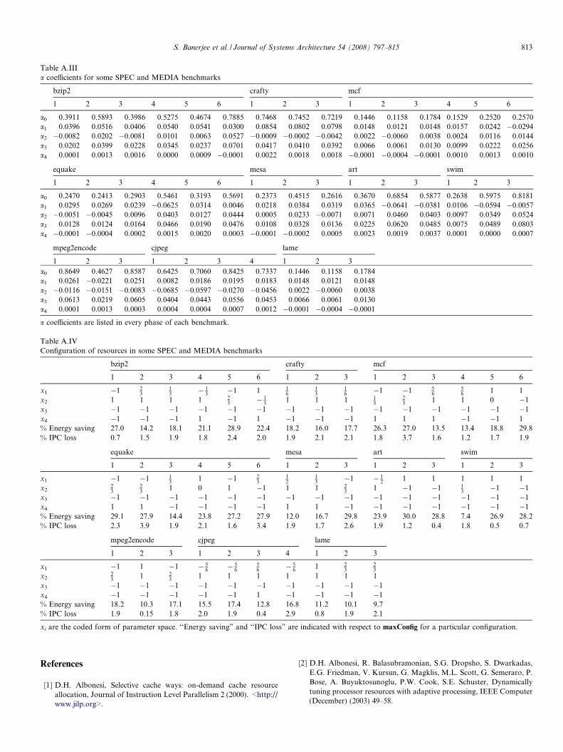
Table A.IIIa coefficients for some SPEC and MEDIA benchmarks

bzip2 crafty mcf

1 2 3 4 5 6 1 2 3 1 2 3 4 5 6

a0 0.3911 0.5893 0.3986 0.5275 0.4674 0.7885 0.7468 0.7452 0.7219 0.1446 0.1158 0.1784 0.1529 0.2520 0.2570a1 0.0396 0.0516 0.0406 0.0540 0.0541 0.0300 0.0854 0.0802 0.0798 0.0148 0.0121 0.0148 0.0157 0.0242 �0.0294a2 �0.0082 0.0202 �0.0081 0.0101 0.0063 0.0527 �0.0009 �0.0002 �0.0042 0.0022 �0.0060 0.0038 0.0024 0.0116 0.0144a3 0.0202 0.0399 0.0228 0.0345 0.0237 0.0701 0.0417 0.0410 0.0392 0.0066 0.0061 0.0130 0.0099 0.0222 0.0256a4 0.0001 0.0013 0.0016 0.0000 0.0009 �0.0001 0.0022 0.0018 0.0018 �0.0001 �0.0004 �0.0001 0.0010 0.0013 0.0010


1 2 3 4 5 6 1 2 3 1 2 3 1 2 3

a0 0.2470 0.2413 0.2903 0.5461 0.3193 0.5691 0.2373 0.4515 0.2616 0.3670 0.6854 0.5877 0.2638 0.5975 0.8181a1 0.0295 0.0269 0.0239 �0.0625 0.0314 0.0046 0.0218 0.0384 0.0319 0.0365 �0.0641 �0.0381 0.0106 �0.0594 �0.0057a2 �0.0051 �0.0045 0.0096 0.0403 0.0127 0.0444 0.0005 0.0233 �0.0071 0.0071 0.0460 0.0403 0.0097 0.0349 0.0524a3 0.0128 0.0124 0.0164 0.0466 0.0190 0.0476 0.0108 0.0328 0.0136 0.0225 0.0620 0.0485 0.0075 0.0489 0.0803a4 �0.0001 �0.0004 0.0002 0.0015 0.0020 0.0003 �0.0001 �0.0002 0.0005 0.0023 0.0019 0.0037 0.0001 0.0000 0.0007


1 2 3 1 2 3 4 1 2 3

a0 0.8649 0.4627 0.8587 0.6425 0.7060 0.8425 0.7337 0.1446 0.1158 0.1784a1 0.0261 �0.0221 0.0251 0.0082 0.0186 0.0195 0.0183 0.0148 0.0121 0.0148a2 �0.0116 �0.0151 �0.0083 �0.0685 �0.0597 �0.0270 �0.0456 0.0022 �0.0060 0.0038a3 0.0613 0.0219 0.0605 0.0404 0.0443 0.0556 0.0453 0.0066 0.0061 0.0130a4 0.0001 0.0013 0.0003 0.0004 0.0004 0.0007 0.0012 �0.0001 �0.0004 �0.0001

a coefficients are listed in every phase of each benchmark.

Table A.IVConfiguration of resources in some SPEC and MEDIA benchmarks

bzip2 crafty mcf

1 2 3 4 5 6 1 2 3 1 2 3 4 5 6

x1 �1 23

13 � 1

3 �1 1 16

13

16 �1 �1 5

656 1 1

x2 1 1 1 1 23 � 1

3 1 1 1 13

23 1 1 0 �1

x3 �1 �1 �1 �1 �1 �1 �1 �1 �1 �1 �1 �1 �1 �1 �1x4 �1 �1 �1 1 �1 1 �1 �1 �1 1 1 1 �1 �1 1% Energy saving 27.0 14.2 18.1 21.1 28.9 22.4 18.2 16.0 17.7 26.3 27.0 13.5 13.4 18.8 29.8% IPC loss 0.7 1.5 1.9 1.8 2.4 2.0 1.9 2.1 2.1 1.8 3.7 1.6 1.2 1.7 1.9


1 2 3 4 5 6 1 2 3 1 2 3 1 2 3

x1 �1 �1 13 1 �1 2

312

13 �1 � 1

2 1 1 1 1 1x2

23

23 1 0 1 �1 1 1 2

3 1 �1 �1 13 �1 �1

x3 �1 �1 �1 �1 �1 �1 �1 �1 �1 �1 �1 �1 �1 �1 �1x4 1 1 �1 �1 �1 �1 1 1 �1 �1 �1 �1 �1 �1 �1% Energy saving 29.1 27.9 14.4 23.8 27.2 27.9 12.0 16.7 29.8 23.9 30.0 28.8 7.4 26.9 28.2% IPC loss 2.3 3.9 1.9 2.1 1.6 3.4 1.9 1.7 2.6 1.9 1.2 0.4 1.8 0.5 0.7


1 2 3 1 2 3 4 1 2 3

x1 �1 1 �1 � 56 � 5

656 � 5

6 1 23

23

x223 1 2

3 1 1 1 1 1 1 1x3 �1 �1 �1 �1 �1 �1 �1 �1 �1 �1x4 �1 �1 �1 �1 �1 1 �1 �1 �1 �1% Energy saving 18.2 10.3 17.1 15.5 17.4 12.8 16.8 11.2 10.1 9.7% IPC loss 1.9 0.15 1.8 2.0 1.9 0.4 2.9 0.8 1.9 2.1

xi are the coded form of parameter space. ‘‘Energy saving” and ‘‘IPC loss” are indicated with respect to maxConfig for a particular configuration.


References

[1] D.H. Albonesi, Selective cache ways: on-demand cache resourceallocation, Journal of Instruction Level Parallelism 2 (2000). <http://www.jilp.org>.

[2] D.H. Albonesi, R. Balasubramonian, S.G. Dropsho, S. Dwarkadas,E.G. Friedman, V. Kursun, G. Magklis, M.L. Scott, G. Semeraro, P.Bose, A. Buyuktosunoglu, P.W. Cook, S.E. Schuster, Dynamicallytuning processor resources with adaptive processing, IEEE Computer(December) (2003) 49–58.

http://www.jilp.org

http://www.jilp.org


[3] Y. Bai, R.I. Bahar, A low-power in-order/out-of-order issue queue,ACM Transactions on Architecture and Code Optimization (TACO)1 (2) (2004) 152–179.

[4] R. Balasubramonian, D.H. Albonesi, A. Buyuktosunoglu, S.Dwarkadas, Memory hierarchy reconfiguration for energy andperformance in general-purpose processor architectures, in: Proceed-ings of the 33rd Annual ACM/IEEE International Symposium onMicroarchitecture, December 2000, pp. 245–257.

[5] S. Banerjee, G. Surendra, S.K. Nandy, Program phase directeddynamic cache way reconfiguration for power efficiency, in: 12th Asiaand South Pacific Design Automation Conference, Yokohama,Japan, 2007, pp. 884–889.

[6] S. Borkar, Design challenges of technology scaling, IEEE Micro 19(4) (1999) 23–29.

[7] D. Brooks, V. Tiwari, M. Martonosi, Wattch: A framework forarchitectural-level power analysis and optimization, InternationalSymposium of Computer Architecture (2000) 83–94.

[8] D. Burger, T.M. Austin, S. Bennet, Evaluating future microproces-sors: the SimpleScalar tool set, University of Wisconsin – Madison,Technical Report CS-TR-96-1308, 1998.

[9] A. Buyuktosunoglu, D.H. Albonesi, P. Bose, P.W. Cook, Tradeoffs inpower efficient issue queue design, in: International Symposium onLow Power Electronics and Design, August 2002, pp. 184–189.

[10] P. Denning, S. Schwartz, Properties of the working set model,Communications of the ACM 15 (3) (1972) 191–198.

[11] P.J. Denning, The working set model for program behaviour,Communications of the ACM 11 (5) (1968) 323–333.

[12] A. Dhodapkar, J.E. Smith, Tuning reconfigurable microarchitecturesfor power efficiency, in: 18th International Parallel and DistributedProcessing Symposium, 2004.

[13] A. Dhodapkar, J.E. Smith, Managing multi-configuration hardwarevia dynamic working set analysis, in: Proceedings of the 29th AnnualInternational Symposium on Computer Architecture, 2002, pp. 233–244.

[14] E. Duesterwald, C. Cascaval, S. Dwarkadas, Characterizing andpredicting program behavior and its variability, in: Proceedings ofParallel Architecture and Compilation Technique, 2003, pp. 220–231.

[15] D. Folegnani, A. Gonzalez, Energy-effective issue logic, in: Proceed-ings of the International Symposium on Computer Architecture,2001, pp. 230–239.

[16] M. Gowan, L. Brio, B. Jackson, Power considerations in the design ofthe alpha 21264 microprocessor, in: Proceedings of the 35th DesignAutomation Conference, 1998, pp. 726–731.

[17] M. Guthaus et al., Mibench: A free, commercially representativeembedded benchmark suite, in: IEEE 4th Annual Workshop onWorkload Characterization, December 2001, pp. 3–14.

[18] M.C. Huang, J. Renau, J. Torrellas, Positional adaptation ofprocessors: application to energy reduction, in: 30th InternationalSymposium on Computer Architecture, 2003, pp. 157–168.

[19] A. Iyer, D. Marculescu, Power aware microarchitecture resourcescaling, in: Proceedings of the Conference on Design, Automation,and Test in Europe, Munich, Germany, 2001, pp. 190–196.

[20] R.K. Jain, The Art of Computer Systems Performance Analysis:Techniques for Experimental Design, Measurement, Simulation, andModeling, John Wiley, New York, 1991.

[21] P.J. Joseph, K. Vaswani, M.J. Thazhuthaveetil, Construction and useof linear regression models for processor performance analysis, in:Proceedings of the International Symposium on High PerformanceComputer Architecture, 2006, pp. 99–108.

[22] P.J. Joseph, K. Vaswani, M.J. Thazhuthaveetil, A predictive perfor-mance model for superscalar processors, in: Proceedings of theInternational Symposium on Microarchitecture, 2006, pp. 161–170.

[23] T. Karkhanis, J.E. Smith, A first-order model of superscalarprocessors, in: Proceedings of the 31st Annual International Sympo-sium on Computer Architecture, 2004, pp. 338–349.

[24] A.J. KleinOsowski, D.J. Lilja, Minnespec: A new spec benchmarkworkload for simulation-based computer architecture research,Computer Architecture Letters 1 (1) (2002) 7.

[25] J. Lau, S. Schoenmackers, B. Calder, Transition phase classificationand prediction, in: 11th International Symposium on High Perfor-mance Computer Architecture, 2005, pp. 278–289.

[26] B. Lee, D. Brooks, Accurate and efficient regression modeling formicroarchitectural performance and power prediction, in: Interna-tional Conference on Architectural Support for Programming Lan-guages and Operating Systems, 2006.

[27] S. Majumdar, R.B. Bunt, Measurement and analysis of localityphases in file referencing behaviour, in: Proceedings of the 1986ACM SIGMETRICS Joint International Conference on Com-puter Performance Modelling, Measurement and Evaluation,1986, pp. 180–192.

[28] The mathworks. <http://www.mathworks.com/>.[29] D.C. Montgomery, Design and Analysis of Experiments, John Wiley,

New York, 2005.[30] D.B. Noonburg, J.P. Shen, Theoretical modeling of superscalar

processor performance, in: Proceedings of the 27th InternationalSymposium on Microarchitecture, 1994, pp. 52–62.

[31] D. Ponomarev, G. Kucuk, O. Ergin, K. Ghose, P. Kogge, Energy-efficient issue queue design, IEEE Transactions on VLSI Systems 11(5) (2003) 789–800.

[32] P. Ranganathan, S. Adve, N.P. Jouppi, Reconfigurable caches andtheir application to media processing, in: Proceedings of the 27thInternational Symposium on Computer Architecture, 2000, pp. 214–224.

[33] J.S. Seng, D.M. Tullsen, Architecture level power optimization –what are the limits? Journal of Instruction Level Parallelism 7(January) (2005). <http://www.jilp.org>.

[34] T. Sherwood, E. Perelman, B. Calder, Basic block distributionanalysis to find periodic behavior and simulation points in applica-tions, in: International Conference on Parallel Architectures andCompilation Techniques, September 2001, pp. 3–14.

[35] T. Sherwood, S. Sair, B. Calder, Phase tracking and prediction, in:Proceedings of International Symposium on Computer Architecture,2003, pp. 336–349.

[36] V. Tiwari, S. Malik, A. Wolfe, M.T.-C. Lee, Instruction levelpower analysis and optimization of software, in: Proceedings ofthe Ninth International Conference on VLSI Design, 1996, pp.326–328.

[37] F. Vandeputte, L. Eeckhout, K.D. Bosschere, A detailed study onphase predictors, in: Euro-Par Conference, 2005, pp. 571–581.

[38] J.J. Yi, D.J. Lilja, D.M. Hawkins, A statistically rigorous approachfor improving simulation methodology, in: International Symposiumon High-Performance Computer Architecture, 2003, pp. 281–291.

[39] Y. Zang, D. Parikh, K. Sankaranarayanan, K. Skadron, M. Stan,Hotleakage: A temperature aware model of subthreshold and gateleakage for architects, Technical Report CS 2003-2005, Departmentof Computer Science, University of Virginia, 2003.

Subhasis Banerjee is currently working at Cor-porate Technology Group in Intel, India. Hereceived Ph.D. from the Indian Institute or Sci-ence in 2007. He received B.Tech and M.Techfrom University of Calcutta in 1998 and 2000. Hisresearch interest includes processor microarchi-tecture, performance modeling and optimizationof computer systems, energy efficient architecture,security in computing platform.

http://www.mathworks.com/

http://www.jilp.org


Surendra Guntur is currently working in NXPSemiconductors. He obtained his Masters andPh.D. from the Indian Institute of Science, Ban-galore in 2001 and 2006 respectively. His researchinterests include computer architecture, perfor-mance modeling and low power and low tem-perature processor design and simulation. He wasa postdoctoral researcher at IRISA/INRIAFrance.

S.K. Nandy is Professor at the SupercomputerEducation and Research Center of the IndianInstitute of Science. His current research addres-ses important issues in micro-architectural opti-mizations for power and performance in ChipMultiprocessors (CMPs), Multiprocessor SoCs(MP-SoCs), and Synthesis of PolymorphicASICs. He has over 100 research publications ininternational journals and proceedings of inter-national conferences.

on the effectiveness of phase based regression models to trade power and performance using dynamic...

Documents