On the Estimation and Application

of Max-Stable Processes

Zhengjun Zhang

Department of Mathematics

Washington University

Saint Louis, MO 63130-4899

USA

Richard L. Smith

Department of Statistics

University of North Carolina

Chapel Hill, NC 27599-3260

USA

January 11, 2004

Abstract

Modeling extreme observations in multivariate time series is a difficult exercise. Classicaltreatments of multivariate extremes use certain multivariate extreme value distributions to modelthe dependencies between components. An alternative approach based on multivariate max-stableprocesses enables the simultaneous modeling of dependence within and between time series. Wepropose a specific class of max-stable processes, known as multivariate maxima of moving maxima(M4 processes for short), and present procedures to estimate their coefficients. To illustrate themethods, some examples are given for modeling jumps in returns in multivariate financial timeseries. We introduce a new measure to quantify and predict the extreme co-movements in pricereturns.

Keywords: multivariate extremes, multivariate maxima of moving maxima, extreme value dis-tribution, empirical distribution, estimation, extreme dependence, extreme co-movement.

0

1 Introduction

Why do we study max-stable process modeling? This question can be answered in several mainaspects regarding theory and modeling of extreme events. In real data analysis, studies have shownthat time series data from finance, insurance and environment etc. are fat-tailed and clustered whenextremal events occur. It has been believed among financial statisticians that multivariate normalmodels are not sufficient in modeling large financial returns and computing value at risk (VaR).Some of the main purposes of studying extreme events are to understand extremal financial risk andextremal co-movements of financial assets. It is obvious that a single distribution fitting is not enoughto characterize those extremal co-movements and that stochastic processes which characterize thelarge jumps and extremal co-movements are needed. In modeling multivariate extremes, especiallyextremal observations in multivariate time series, there are still several important issues to be solved.These issues include the model applicability, tractability of model parameters, etc. Besides theseissues, there are needs for improving theories and methodologies in extreme value theory itself.

In the aspects of traditional approaches studying extremes, univariate extreme value theorystudies the limiting distribution of the maxima or the minima of a sequence of random variables.There are well-developed approaches to model univariate extremal processes. Galambos (1987),Leadbetter, Lindgren and Rootzen (1983), and Resnick (1987) are excellent reference books onthe probabilistic side. Coles (2001) and Smith (2003) have reviewed statistical methodology forextremes. Embrechts, Kluppelberg, and Mikosch (1997) give an excellent viewpoint of modelingextremal events. These references and others are important sources for applying extreme valuetheory, but problems concerning the environment, finance and insurance etc. are multivariate incharacter: for example, floods may occur at different sites along a coastline; the failure of a portfoliomanagement may be caused by a single extremal price movement or multiple movements. Heremultivariate extreme modeling is essential for risk management and precision of modeling.

In the multivariate context, the maximum is taken componentwise and there is no unified para-metric type of limiting distribution. However, there have been many characterizations of the possiblelimits, such as de Haan and Resnick (1977), de Haan (1985), and Resnick’s (1987) point processapproach, and Pickands’s (1981) representation theorem for multivariate extreme value distribu-tion with unit exponential margins. If a limiting multivariate extreme value distribution exists, itsmarginal distributions must be one of the three types of univariate extreme value distributions ifthey are non-degenerate. Many different models are reviewed by Coles and Tawn (1991, 1994).

In many circumstances, extremal observations appear to be clustered in time. For example, largeprice movements in the stock market, large insurance claims after a disaster event, heavy rainfallsetc., may persist over several observations. Neither univariate nor multivariate extreme value theoryis adequate to describe this kind of clustering of extreme events in a time series.

Max-stable processes, introduced by de Haan (1984), are an infinite-dimensional generalizationof extreme value theory which does have the potential to describe clustering behavior. The limit-ing distributions of univariate and multivariate extreme value theory are max-stable, as shown byLeadbetter et al. (1983) in the univariate case and Resnick (1987) in the multivariate case. One ofthe most important features of max-stable processes is that they not only model the cross-sectionaldependence, but also model the dependence across time.

Parametric models for max-stable processes have been considered since the 1980s. Deheuvels

1

(1983) defines the moving minimum (MM) process. Davis and Resnick (1989) study what they callthe max-autoregressive moving average (MARMA) process of a stationary process. For prediction,see also Davis and Resnick (1993). Recently, Hall, Peng, and Yao (2002) discuss moving maximummodels. For a finite number of parameters, they propose parameter estimators based on empiricaldistribution functions. In the study of characterization and estimation of the multivariate extremalindex introduced by Nandagopalan (1991, 1994), Smith and Weissman (1996) extend Deheuvels’definition to the so called multivariate maxima of moving maxima (henceforth M4) process. Smithand Weissman (1996) argue that under quite general conditions, the extreme values of multivariatestationary time series may be characterized in terms of a limiting max-stable process. They also showthat a very large class of max-stable processes may be approximated by M4 processes mainly becausethose processes have the same multivariate extremal indexes as the M4 processes have (Theorem 2.3in Smith and Weissman 1996).

The use of M4 process is a new development in modeling extremal observations of multivariatetime series. Due to the lack of statistical estimation methods, applications of max-stable processesare hardly found in real data analysis. For a class of M4 processes which contain a finite numberof parameters, Zhang and Smith (2003) study the behavior of the specific M4 processes. Theyalso provide guidance of applying M4 process. But, a practically usable approach on estimating allparameters has yet developed. The purpose of this paper is to fill the gaps between the theoreticalprobabilistic results and the real data modeling.

This paper is organized as follows. In Section 2, we introduce the model which is used to modelfinancial data in Section 5. The distributional properties of the model which lead to the constructionof estimating procedures of all parameters are studied. Model identifiability is addressed. Theestimators and their asymptotic properties are studied in Section 3. In contrast to the bootstrappedprocesses which Hall et al. (2002) use to construct confidence intervals and prediction intervals forthe moving maxima models, we directly construct parameter estimators and prove their asymptoticproperties for the M4 processes. In Section 4 we provide simulation examples to show the efficiencyof proposed estimating procedures. In Section 5 we explore modeling financial time series data as M4processes. Stock price returns of General Electric Co. (GE), CITI Group (C) and Pfizer (PFE) arestudied. Parameter estimates of M4 models are based on multivariate time series of approximately5000 days data. In Section 6, some discussions are addressed. Technical arguments are shown inSection 7.

2 The model and its identifiability

Suppose we have multivariate time series {Xid, i = 0,±1,±2, ..., d = 1, ..., D}, where i is time and d

indexes a component of the process. Initially, we assume that the D-dimensional process is stationaryin time but make no other assumptions.

Well-established methods of univariate extreme value theory (see Coles (2001) or Smith (2003)for reviews) show that under very mild assumptions, it is possible to model the behavior of a randomvariable above a high threshold by the generalized Pareto distribution. Assuming this and applyinga probability integral transformation, it is possible to transform each marginal distribution of theprocess, above a high threshold, so that the marginal distribution is unit Frechet. For the moment weignore the high threshold part of the modeling, and assume that the univariate Frechet assumption

2

applies to the whole distribution. Thus, we transform each Xid into a random variable Yid for whichPr{Yid ≤ y} = exp(−1/y), 0 < y < ∞.

The process {Yid} is said to be max-stable if for any finite collection of time points i = i1, i1 +1, ..., i2 and any positive set of values {yid, i = i1, ..., i2, d = 1, ..., D}, we have

Pr{Yid ≤ yid, i = i1, ..., i2, d = 1, ..., D} = [Pr{Yid ≤ nyid, i = i1, ..., i2, d = 1, ..., D}]n .

This property directly generalizes the max-stability property of univariate and multivariate extremevalue distributions (Leadbetter et al. (1983), Resnick (1987)) and provides a convenient mathematicalframework to talk about extremes in infinite-dimensional processes. From now on, we shall assumethat our multivariate time series, after marginal transformation to unit Frechet, is max-stable.

The next task is to characterize max-stable processes. For univariate processes, such a charac-terization was provided by Deheuvels (1983). This was generalized by Smith and Weissman (1996)to the following: under some mixing assumptions that we shall not detail here, any max-stable pro-cess with unit Frechet margins may be approximated by a multivariate maxima of moving maximaprocess, or M4 for short, with the representation

Yid = maxl=1,2,...

max−∞<k<∞

al,k,dZl,i−k, −∞ < i < ∞, d = 1, ..., D,

where {Zl,i, l = 1, 2, ...,−∞ < i < ∞} are independent unit Frechet random variables and al,k,d arenon-negative coefficients satisfying

∑∞l=1

∑∞k=−∞ al,k,d = 1 for each d.

In practice, even this representation is too cumbersome for practical application, involving in-finitely many parameters al,k,d, so we simplify it by assuming that only a finite number of thesecoefficients are non-zero. Thus we have the representation

Yid = max1≤l≤Ld

max−K1ld≤k≤K2ld

al,k,dZl,i−k, −∞ < i < ∞, d = 1, . . . , D, (2.1)

where Ld, K1ld, K2ld are finite and the coefficients satisfy∑Ld

l=1

∑K1ldk=−K1ld

al,k,d = 1 for each d.Under model (2.1), when an extremal event occurs or when a large Zli occurs, Yid ∝ al,i−k,d for

i ≈ k, i.e. if some Zlk is much larger than all neighboring Z values, we will have Yid = al,i−k,dZlk

for i near k. This indicates a moving pattern of the time series, known as a signature pattern.Hence Ld corresponds to the maximum number of signature patterns. The constants K1ld and K2ld

characterize the range of dependence in each sequence and (maxl K1ld +maxl K2ld +1) is the order ofthe moving maxima processes. We illustrate these phenomena in Figure 1. Plots (b) and (c) involvethe same values of (al,−K1ld,d, al,−K1ld+1,d, . . . , al,K2ld,d), i.e. the same single value l = l1. Similarly,Plots (d) and (e) involve the same values of (al,−K1ld,d, al,−K1ld+1,d, . . . , al,K2ld,d), i.e. the samesingle value l = l2. One can see immediately that Plot (b) is a blowup of a few observations of theprocess in (a) and Plot (c) is a similar blowup of a few other observations of the process in (a). Thevertical coordinate scales of Y in Plot (b) are from 0 to 20, while the vertical coordinate scales of Y

in Plot (c) are from 0 to 100. Similar interpretations can be applied to Plots (d)-(e). These plotsshow that there are characteristic shapes around the local maxima that replicate themselves. Thoseblowups, or replicates, are known as signature patterns.

Under model (2.1), it is easy to obtain the finite distribution of {Yid, 1 ≤ i ≤ r, 1 ≤ d ≤ D}.The goal is to estimate all parameters {al,k,d} under the constraints that the parameters are positive

3

0 100 200 300 4000

10

20

30

40

50

60

70

80

90

100(a)

41 42 43 44 45 460

2

4

6

8

10

12

14

16

18

20(b)

102 103 104 105 106 1070

10

20

30

40

50

60

70

80

90

100(c)

256 257 258 259 260 2610

10

20

30

40

50

60

70

80

90

100(d)

312 313 314 315 316 3170

5

10

15

20

25

30

35(e)

Figure 1: A demonstration of a M4 process. (a) is a simulated 365 days data for a componentprocess. (b) - (e) are partial pictures drawn from the whole simulated data showing two differentmoving patterns, called signature patterns, in certain time periods when extremal events occur.

4

and the summation is equal to 1 for each d = 1, . . . , D. Due to the degeneracy of the multivariatejoint distribution function of the M4 processes, the method of maximum likelihood is in general notapplicable in this instance. In some simple cases, for example Ld = 2, K1ld = K2ld = 0, the methodof maximum likelihood can be applied – see Zhang (2003). The estimators developed in this paperare based on the joint empirical distribution functions.

It follows immediately from that

Pr(Yid ≤ y) = e−1/y, (2.2)

Pr(Yid ≤ yid, Yi+1,d ≤ yi+1,d) = exp[−

Ld∑

l=1

2+K1ld∑

m=1−K2ld

max{al,1−m,d

yid,al,2−m,d

yi+1,d

}], (2.3)

Pr(Y1d ≤ y1d, Y1d′ ≤ y1d′) = exp[−

max(Ld,Ld′ )∑

l=1

1+max(K1ld,K1ld′ )∑

m=1−max(K2ld,K2ld′ )

max{al,1−m,d

y1d,al,1−m,d′

y1d′

}],

(2.4)

and a general joint probability formula:

Pr{Yid ≤ yid, 1 ≤ i ≤ r, 1 ≤ d ≤ D} = exp[−

maxd Ld∑

l=1

r+maxd K1ld∑

m=1−maxd K2ld

max1−m≤k≤r−m

max1≤d≤D

al,k,d

ym+k,d

], (2.5)

where al,k,d = 0 when the triple subindex is outside the range defined in Model (2.1). This assumptionis held in the rest of the paper. These formulas are used to compute various probabilities and toconstruct asymptotic covariance matrices in the following sections.

Remark 1 For each l, the value of∑K2ld

k=−K1ldal,k,d tells that what proportions of the total observa-

tions are approximately drawn from the lth signature process in the dth observed process.

It is clear from equations (2.2)-(2.4) that we cannot hope to estimate the M4 parameters based onthe marginal distributions alone. However, there is some hope to estimate those parameters basedon bivariate distributions. This naturally suggests the question of whether bivariate distributionsidentify all the parameters of the process. In the following discussion we propose sufficient, thoughnot necessary, conditions for that.

The probability evaluated at the points (yid, yi+1,d) in (2.3) depends on the comparison ofal,1−m,d/yid and al,2−m,d/yi+1,d, and similarly in (2.4). By fixing one of yid and yi+1,d – say yid, thenal,1−m,d/(al,2−m,dyid) is the change point of max(al,1−m,d/yid, al,2−m,d/yi+1,d) when yi+1,d varies. Itis easy to see the following identity,

Pr{Y1d ≤ u, Y2d ≤ u + x} = Pr{Y1d ≤ 1, Y2d ≤ (u + x)/u}(1/u).

So without loss of generality, we can fix yid = 1 for simplicity of our calculation. In real dataapplication we may choose a threshold value u and fix yid = u or yi+1,d = u.From (2.3) and (2.4), we have

Pr{Y1d ≤ 1, Y2d ≤ x} = exp[−

Ld∑

l=1

2+K1ld∑

m=1−K2ld

max(al,1−m,d,al,2−m,d

x)],

5

and

Pr{Y1d ≤ 1, Y1d′ ≤ x} = exp[−

max(Ld,Ld′ )∑

l=1

1+max(K1ld,K1ld′ )∑

m=1−max(K2ld,K2ld′ )

max(al,1−m,d,

al,1−m,d′

x

)].

Letbd(x) = − log

[Pr(Y1d ≤ 1, Y2d ≤ x)

], bdd′(x) = − log

[Pr(Y1d ≤ 1, Y1d′ ≤ x)

],

we have

bd(x) =Ld∑

l=1

[al,K2ld,d + max(al,K2ld−1,d,

al,K2ld,d

x) + max(al,K2ld−2,d,

al,K2ld−1,d

x) (2.6)

+max(al,K2ld−3,d,al,K2ld−2,d

x) + · · ·+ max(al,−K1ld,d,

al,−K1ld+1,d

x) +

al,−K1ld,d

x

],

d = 1, . . . , D,

and

bdd′(x) =max(Ld,Ld′ )∑

l=1

1+max(K1ld,K1ld′ )∑

m=1−max(K2ld,K2ld′ )

max(al,1−m,d,al,1−m,d′

x). (2.7)

It is clear that for each d, qd(x) , xbd(x) and qdd′(x) , xbdd′(x) are piecewise linear functions andhave slope jump points at al,j,d/al,j′,d or al,k,d/al,k,d′ , where the notation A , B means that A isdenoted as B. This suggests that if we can identify the functions qd(x) or qdd′(x), we may be ableto identify all the parameters al,k,d. A typical qd(x) picture is shown in Figure 2.

0 0.5 1 1.5 2 2.5 30

0.5

1

1.5

2

2.5

3

3.5

x

q(x)

A typical q(x) picture

Figure 2: A demonstration of qd(x) and its slope q′d(x) and slope change points.

The following propositions will show the identifiability. The proofs of propositions 2.2, 2.3, 2.4are deferred to Section 7.

Proposition 2.1 For a fixed d and Ld = 1, if all(K1+K2+1

2

)ratios ajd

aj′dare distinct, the model is

uniquely identified by qd(x), or bd(x).

The reason why Proposition 2.1 is true is that in this case, any permutation of the ajd’s must createa new set of values of ratios or jump points which will result in a different function of qd(x).

6

Remark 2 This justifies statements like “for almost all (w.r.t Lebesgue measure) choices of coeffi-cients a−K1ld,d, . . . , aK2ld,d, the model is identifiable from qd(x).”

Remark 3 The uniqueness means the values of the vector (a−K1ld,d, a−K1ld+1,d, . . . , aK2ld,d) areuniquely determined, but their locations (determined by K1ld and K2ld) are not as shown in thefollowing two processes.

Yi = max(.2Zi−1, .3Zi, .5Zi+1),

Y ′i = max(.2Zi, .3Zi+1, .5Zi+2).

But we can shift the whole vector of the second process to get the first process. There should beno ambiguity that we treat them as one model since they have the same joint distribution functionswithin each sequence, while they generate different sample paths.

Proposition 2.2 For a fixed d, if all(K1ld+K2ld+1

2

)ratios al,j,d

al,j′,d, l = 1, . . . , Ld, j 6= j′, are distinct,

the model is uniquely identified by qd(x), or bd(x).

Remark 4 For a fixed d, by uniqueness we mean that if {al,k,d, l = 1, . . . , Ld, −K1ld ≤ k ≤K2ld} and {a′l′,k,d, l′ = 1, . . . , Ld, −K1l′d ≤ k ≤ K2l′d} are two sets of solutions, they must satisfythe condition: a′m(l),k,d = al,k,d, l = 1, . . . , Ld, where {m(l), l = 1, . . . , Ld} is a permutation of{1, . . . , Ld}. For example, we consider the following two structures of parameter values are equivalent:

(alkd) =

[1/4 1/61/4 1/3

], (a′lkd) =

[1/4 1/31/4 1/6

]

for a fixed d (in the above two matrices, we use l as row indexes and k as column indexes) since theyresult in the same joint distributions, but different sample paths. It is easy to see that the ratios are3/2, 2/3, 4/3, 3/4 in this example. All the ratios are distinct. For higher dimensional structures,we can have similar equivalences as long as they have the same joint distributions.

Remark 5 By Remark 4, the solutions from bd(x) can be something like either (alkd) or (a′l′kd),and the solutions from bd′(x) can be something like either (alkd′) or (a′l′kd′). While parameter valuescan be determined by bd(x) for each d, functions bd(x) are not enough to determine the parameterstructures in M4 processes. For example, one may obtain the following coefficients

(alkd) =

[1/4 1/61/4 1/3

], (alkd′) =

[1/8 1/41/4 3/8

],

based on observations from a bivariate process and functions bd(x), bd′(x), but one may also obtainthe following coefficients

(a′lkd) =

[1/4 1/31/4 1/6

], (a′lkd′) =

[1/8 1/41/4 3/8

],

based on the same observations and functions bd(x), bd′(x). Obviously, M4 models formed usingthese two sets of coefficients are two different models since the joint distributions are different andthe bivariate sample paths are different. The purpose of functions bdd′(x) is to find which structureis the true structure.

7

Proposition 2.3 Suppose all ratios al,j,d

al,j′,dfor all l and j 6= j′ are distinct, all ratios

al,j,d′al,j′,d′

for all l

and j 6= j′ are distinct, and all nonzero and existing ratios al,k,d

al,k,d′for all l and k are distinct when

d 6= d′, then

bd(x) =∑Ld

l=1

[al,K2ld,d + max(al,K2ld−1,d,

al,K2ld,d

x ) + max(al,K2ld−2,d,al,K2ld−1,d

x )

+max(al,K2ld−3,d,al,K2ld−2,d

x ) + · · ·+ max(al,−K1ld,d,al,−K1ld+1,d

x ) + al,−K1ld,d

x

],

bd′(x) =∑Ld′

l=1

[al,K2ld′ ,d′ + max(al,K2ld′−1,d′ ,

al,K2ld′ ,d′x ) + max(al,K2ld′−2,d′ ,

al,K2ld′−1,d′x )

+max(al,K2ld′−3,d′ ,al,K2ld′−2,d′

x ) + · · ·+ max(al,−K1ld′ ,d′ ,al,−K1ld′+1,d′

x ) +al,−K1ld′ ,d′

x

],

bdd′(x) =max(Ld,Ld′ )∑

l=1

1+max(K1ld,K1ld′ )∑m=1−max(K2ld,K2ld′ )

max(al,1−m,d,al,1−m,d′

x ),

(2.8)

uniquely determine all values of al,k,d and al,k,d′ for any two fixed d and d′.Furthermore, there exist points x1, x2, . . . , xm, m ≤ ∑

d

∑Ldl (K1ld + K2ld + 2), such that

bd(xi) and bdd′(xi), i = 1, . . . , m,

uniquely determine all values of al,k,d and al,k,d′ for any two fixed d and d′.

Proposition 2.4 Suppose all ratios al,j,d

al,j′,dfor all l and j 6= j′ are distinct for each d = 1, . . . , D, and

nonzero and existing ratios al,k,1

al′,k,d′for all l, l′ and k are distinct for each d′ = 2, . . . , D, then

bd(x) =∑Ld

l=1

[al,K2ld,d + max(al,K2ld−1,d,

al,K2ld,d

x ) + max(al,K2ld−2,d,al,K2ld−1,d

x )

+max(al,K2ld−3,d,al,K2ld−2,d

x ) + · · ·+ max(al,−K1ld,d,al,−K1ld+1,d

x ) + al,−K1ld,d

x

],

d = 1, . . . , D,

b1d′(x) =max(L1,Ld′ )∑

l=1

1+max(Kl11,K1ld′ )∑m=1−max(Kl21,K2ld′ )

max(al,1−m,1,al,1−m,d′

x ), d′ = 2, . . . , D,

uniquely determine all values of al,k,d, d = 1, . . . , D, l = 1, . . . , Ld, −K1ld ≤ k ≤ K2ld.Furthermore, there exist points x1, x2, . . . , xm, m ≤ (2D−1)

∑d

∑Ldl (K1ld +K2ld +2)+2D, such

thatbd(xi) and b1d′(xi), i = 1, . . . ,m, d = 1, . . . , D, d′ = 2, . . . , D

uniquely determine all values of al,k,d.

Remark 6 Only b1d′(x) is used in the proof of model identifiability. In some situations, other bdd′(x)functions may also be needed in order to prove identifiability or to get estimates of all parameters.

Since we want to construct the estimators of parameters in model (2.1) based on the bivariatedistribution, we know that from the previous arguments, if the conditions are false, we may not beable to identify the model. But we may be able to identify the model via some higher-order jointdistribution. We now construct an artificial example to demonstrate this idea.

Example 2.1 This is a counterexample to show a process that is not identifiable via the bivariatejoint distribution, but can be identifiable from the trivariate joint distribution.

8

Let (a0, . . . , a4) = 16(1, 1, 2, 1, 1) and (b0, . . . , b4) = 1

6(1, 2, 1, 1, 1). We consider the two processesgenerated by the sequences a0, . . . , a4 and b0, . . . , b4, i.e.

Yi = maxk=0,1,2,3,4

akZi−k, −∞ < i < ∞,

Y ′i = max

k=0,1,2,3,4bkZi−k, −∞ < i < ∞.

Then the number of slope change points is p = 3,and the slope change points are r1 = 12 , r2 = 1, r3 = 2

for both configurations, so q(x) is the same and displayed in Figure 2 with

q′(x) =

16 0 < x < 1

2 ,12

12 < x < 1,

56 1 < x < 2,

1 2 < x

i.e. we can’t distinguish the ai’s from the bi’s on the basis of q(x). However, consider the formula

− log(Pr(Y1 ≤ y1, Y2 ≤ y2, Y3 ≤ y3)) = a4y1

+ max(a3y1

, a4y2

) + max(a2y1

, a3y2

, a4y3

)+max(a1

y1, a2

y2, a3

y3) + max(a0

y1, a1

y2, a2

y3)

+max(a0y2

, a1y3

) + a0y3

and let y1 = 1, y2 = y3 = c where c > 2, then

− log(Pr(Y1 ≤ y1, Y2 ≤ y2, Y3 ≤ y3)) =16[1 + 1 + 2 + 1 + 1 +

1c

+1c] = 1 +

13c

,

and similarly

− log(Pr(Y ′1 ≤ y1, Y

′2 ≤ y2, Y

′3 ≤ y3)) =

16[1 + 1 + 1 + 2 + 1 +

2c

+1c] = 1 +

12c

,

So the two values of Pr(Y1 ≤ y1, Y2 ≤ y2, Y3 ≤ y3) and Pr(Y ′1 ≤ y1, Y

′2 ≤ y2, Y

′3 ≤ y3) are distinct in

this case.

In other words, the two possible models are distinguishable from their trivariate distributions, butnot bivariate. However this is a specific example where we need trivariate distribution function, inmost cases bivariate distributions are enough.

3 The estimators and asymptotics

We now propose estimators for parameters in general M4 processes. It is known that an empiricalprocess approximates a random process from which observations are obtained. Our estimators aremotivated from such approximations of one process to the other one.Let x1d, ..., xLd, x

′1d, ..., x

′Ld be positive constants which, for the moment, are arbitrary. Let A1d =

(0, x1d)× (0, x′1d), . . . , AL−1,d = (0, xL−1,d)× (0, x′L−1,d) be different sets. Define

ΥAjd=

1n

n∑

i=1

IAjd(Yid, Yi+1,d), (3.1)

9

where IA(.) is an indicative function. Then by the strong law of large numbers (SLLN), we have

ΥAjd

a.s.−→ Pr{Ajd} = Pr{Y1d ≤ xjd, Y2d ≤ x′jd} , µjd. (3.2)

Formulas (3.1) and (3.2) are used to construct the estimators for parameters and to show the centrallimit theorem (CLT) of the estimators. In order to study asymptotic normality, we apply the followingproposition which is Theorem 27.4 in Billingsley (1995). First we introduce the so-called α-mixingcondition.

For a sequence ζ1, ζ2, ... of random variables, let αn be a number such that

| Pr(A ∩B)− Pr(A) Pr(B) |≤ αn

for A ∈ σ(ζ1, ..., ζk), B ∈ σ(ζk+n, ζk+n+1, ...), and k ≥ 1, n ≥ 1. When αn → 0, the sequence {ζn} issaid to be α-mixing. This means that ζk and ζk+n are approximately independent for large n.

Proposition 3.1 Suppose that Υ1, Υ2, . . . , is stationary and α-mixing with αn = O(n−5) and thatE[Υn] = 0 and E[Υ12

n ] < ∞. If Sn = Υ1 + · · ·+ Υn, then

n−1Var[Sn] → σ2 = E[Υ21] + 2

∞∑

k=1

E[Υ1Υ1+k],

where the series converges absolutely. If σ > 0, then Sn/σ√

nL→ N(0, 1).

Remark 7 The conditions αn = O(n−5) and E[Υ12n ] < ∞ are stronger than necessary as stated in

the remark following Theorem 27.4 in Billingsley (1995) to avoid technical complication in the proof.

Let Υnd = IAjd{Ynd, Yn+1,d} − µjd, then E[Υnd] = 0 and E[Υ12

nd] < ∞ because Υnd is bounded.The α-mixing condition is satisfied since Ynd’s are M -dependent. So the conditions of Proposition3.1 are satisfied. As one can see that even though the conditions of Proposition 3.1 are stronger thanneeded for the CLT result, they are plenty strong enough for the application in this paper. By usingBillingsley’s arguments, we have the following two lemmas whose proofs are deferred to Section 7.

Lemma 3.2 Suppose that ΥAjdand µjd are defined in (3.1) and (3.2) respectively, if σjd > 0, then

√n(ΥAjd

− µjd)L−→ N(0, σ2

jd),

where µjd is the mean of random variable ΥAjd. Its value is defined in (3.2). The value of σ2

jd isdefined as:

σ2jd = µjd−µ2

jd +2maxl K1ld+maxl K2ld+1∑

k=1

[Pr

{Y1d ≤ xjd, Y2d ≤ x′jd, Y1+k,d ≤ xjd, Y2+k,d ≤ x′jd

}−µ2jd

].

A generalization of Lemma 3.2 to multivariate asymptotics is shown in the following lemma.

Lemma 3.3 Suppose that ΥAjdand µjd are defined in (3.1) and (3.2) respectively, then

√n

ΥA1d

...ΥAL−1,d

−

µ1d...

µL−1,d

L−→ N

(0,Σd +

maxl K1ld+maxl K2ld+1∑

k=1

{Wkd + W Tkd}

)

10

where the entries σi,j,d of matrix Σd are defined by: µi,j,d = Pr{Y1d ≤ min(xid, xjd), Y2d ≤ min(x′id, x′jd)},

σi,j,d = µi,j,d − µidµjd, the matrix Wkd has entries wijkd = Pr(Y1d ≤ xid, Y2d ≤ x′id, Y1+k,d ≤

xjd, Y2+k,d ≤ x′jd)− µidµjd, µi,i,d = µid.

The above constructions are for a component process. We now turn to constructions for multivariate(vector) processes. A generalization of Lemma 3.3 to the empirical counterparts of bd(x) and b1d′(x)can be realized. The empirical counterparts of bd(x) and b1d′(x) are defined as:

Ud(x) =1n

n∑

i=1

I{Yid≤1, Yi+1,d≤x}, bd(x) = − log[Ud(x)

], d = 1, . . . , D, (3.3)

U1d′(x) =1n

n∑

i=1

I{Yi1≤1, Yid′≤x}, b1d′(x) = − log[U1d′(x)

], d′ = 2, . . . , D. (3.4)

Letx1d, x2d, . . . , xmd, d = 1, . . . , D,

where m ≤ (2D − 1)(maxl K1ld + maxl K2ld + 1) + 2D as described in Proposition 2.4, and

x′1d′ , x′2d′ , . . . , x′m′d′ , d′ = 2, . . . , D,

where m′ ≤ (2D−1)∑

d

∑Ldl (K1ld +K2ld +2)+2D, be suitable choice of the points used to evaluate

the values of all functions defined. Then (3.3) and (3.4) can be written as the following vector forms:

x =(x11, x21, . . . , xm1, x12, . . . , xmD, x′12, x′22, . . . , x′m′2, x′13, . . . , x′m′D

)T,

U =�U1(x11), . . . , U1(xm1), U2(x12), . . . , UD(xmD), U12(x

′12), . . . , U12(x

′m′2), . . . , U1D(x′m′D)

�T

,

bb =�bb1(x11), . . . , bb1(xm1), bb2(x12), . . . , bbD(xmD), bb12(x

′12) , . . . , bb12(x

′m′2), . . . , bb1D(x′m′D)

�T

.

In order to obtain the joint asymptotics of U and the joint asymptotics of b, the following notationsand results will be used. They play similar roles as those of µi,j,d and σi,j,d in Lemma 3.3. Thesenotations and their expressions are:

µdjd = E[Ud(xjd)

]= Pr(Y1d ≤ 1, Y2d ≤ xjd),

d = 1, . . . , D, j = 1, . . . ,m,

µ1d′j′d′ = E[U1d′(x′j′d′)

]= Pr(Y11 ≤ 1, Y1d′ ≤ x′j′d′),

d′ = 2, . . . , D, j′ = 1, . . . ,m′,

µdjd, d′j′d′ = E[(

I{Y1d≤1,Y2d≤xjd} − µdjd

)(I{Y1d′≤1,Y2d′≤xj′d′} − µd′j′d′

)]

= Pr(Y1d ≤ 1, Y2d ≤ xjd, Y1d′ ≤ 1, Y2d′ ≤ xj′d′)− µdjdµd′j′d′ ,

d, d′ = 1, . . . , D, j, j′ = 1, . . . , m,

µdjd, 1d′j′d′ = E[(

I{Y1d≤1,Y2d≤xjd} − µdjd

)(I{Y11≤1,Y1d′≤x′

j′d′} − µ1d′j′d′)]

= Pr(Y1d ≤ 1, Y2d ≤ xjd, Y11 ≤ 1, Y1d′ ≤ x′j′d′)− µdjdµ1d′j′d′ ,

d = 1, . . . , D, j = 1, . . . ,m,

d′ = 2, . . . , D, j′ = 1, . . . , m′,

11

µ1d′j′d′, djd = E[(

I{Y11≤1,Y1d′≤x′j′d′} − µ1d′j′d′

)(I{Y1d≤1,Y2d≤xjd} − µdjd

)]

= Pr(Y1d ≤ 1, Y2d ≤ xjd, Y11 ≤ 1, Y1d′ ≤ x′j′d′)− µdjdµ1d′j′d′

= µdjd, 1d′j′d′ ,

d = 1, . . . , D, j = 1, . . . , m,

d′ = 2, . . . , D, j′ = 1, . . . , m′,

µ1djd, 1d′j′d′ = E[(

I{Y11≤1,Y1d≤x′jd} − µ1djd

)(I{Y11≤1,Y1d′≤x′

j′d′} − µ1d′j′d′)]

= Pr(Y11 ≤ 1, Y1d ≤ x′jd, Y1d′ ≤ x′j′d′)− µ1djdµ1d′j′d′ ,

d = 2, . . . , D, j = 1, . . . , m′,d′ = 2, . . . , D, j′ = 1, . . . , m′,

w(k)djd, d′j′d′ = E

[(I{Y1d≤1,Y2d≤xjd} − µdjd

)(I{Y1+k,d′≤1,Y2+k,d′≤xj′d′} − µd′j′d′

)]

= Pr(Y1d ≤ 1, Y2d ≤ xjd, Y1+k,d′ ≤ 1, Y2+k,d′ ≤ xj′d′)− µdjdµd′j′d′ ,

d, d′ = 1, . . . , D, j, j′ = 1, . . . , m,

w(k)djd, 1d′j′d′ = E

[(I{Y1d≤1,Y2d≤xjd} − µdjd

)(I{Y1+k,1≤1,Y1+k,d′≤x′

j′d′} − µ1d′j′d′)]

= Pr(Y1d ≤ 1, Y2d ≤ xjd, Y1+k,1 ≤ 1, Y1+k,d′ ≤ x′j′d′)− µdjdµ1d′j′d′ ,

d = 1, . . . , D, j = 1, . . . ,m,

d′ = 2, . . . , D, j′ = 1, . . . ,m′,

w(k)1d′j′d′, djd = E

[(I{Y1,1≤1,Y1,d′≤x′

j′d′} − µ1d′j′d′)(

I{Y1+k,d≤1,Y2+k,d≤xjd} − µdjd

)]

= Pr(Y1,1 ≤ 1, Y1,d′ ≤ x′j′d′ , Y1+k,d ≤ 1, Y2+k,d ≤ xjd)− µdjdµ1d′j′d′ ,

d = 1, . . . , D, j = 1, . . . , m,

d′ = 2, . . . , D, j′ = 1, . . . ,m′,

w(k)1djd, 1d′j′d′ = E

[(I{Y11≤1,Y1d≤x′jd} − µ1djd

)(I{Y1+k,1≤1,Y1+k,d′≤x′

j′d′} − µ1d′j′d′)]

= Pr(Y11 ≤ 1, Y1d ≤ x′jd, Y1+k,1 ≤ 1, Y1+k,d′ ≤ x′j′d′)− µ1djdµ1d′j′d′ ,

d = 2, . . . , D, j = 1, . . . , m′,d′ = 2, . . . , D, j′ = 1, . . . ,m′.

The above quantities are not convenient to express a multivariate central limit theorem. We define

12

the following vectors using the notations defined.

µ =

µ111

µ121...

µ1m1

µ212...

µDmD

µ1212

µ1222...

µ12m′2

µ1313...

µ1Dm′D

=

µ1

µ2...

µm

µm+1...

µD×m

µD×m+1

µD×m+2...

µD×m+m′

µD×m+m′+1...

µD×m+(D−1)m′

, b =

b1(x11)b1(x21)

...b1(xm1)b2(x12)

...bD(xmD)b12(x′12)b12(x′22)

...b12(x′m′2)b13(x′13)

...b1D(x′m′D)

.

Notice that the subscripts of the elements of vector µ are different in its two vector forms thoughthe same notation µ is used. To form the above vectors, for example, to get the rth value in thevector µ, we have used the following index transformation:

{µdjd → µr, where r = (d− 1)×m + j,

µ1d′jd′ → µr, where r = D ×m + (d′ − 2)×m′ + j,

where [.] takes integer values. We now use the similar relations between the indexes of µdjd and theindexes of µr to define the following variables:

σrs =

µdjd,d′j′d′ , if r ≤ D ×m, s ≤ D ×m,

µdjd,1d′j′d′ , if r ≤ D ×m, s > D ×m,

µ1djd,d′j′d′ , if r > D ×m, s ≤ D ×m,

µ1djd,1d′j′d′ , if r > D ×m, s > D ×m,

wrsk =

w(k)djd,d′j′d′ , if r ≤ D ×m, s ≤ D ×m,

w(k)djd,1d′j′d′ , if r ≤ D ×m, s > D ×m,

w(k)1djd,d′j′d′ , if r > D ×m, s ≤ D ×m,

w(k)1djd,1d′j′d′ , if r > D ×m, s > D ×m,

and the matrices:Σ = (σrs), Wk = (wrs

k ), Θ = (diag{µ})−1 × (diag{x}).After putting everything above together, the following lemma is obtained. Its proof simply followsarguments used in Lemma 3.3 and the mean value theorem.

13

Lemma 3.4 For the choices of xjd, xj′d′ and with the notations established, we have

√n(U− µ) L−→ N

(0,Σ +

maxl K1ld+maxl K2ld+1∑

k=1

{Wk + W Tk }

),

and√

n(b− b) L−→ N(0, Θ

[Σ +

maxl K1ld+maxl K2ld+1∑

k=1

{Wk + W Tk }

]ΘT

),

which establish the asymptotics for the empirical functions bd(x).

The results in Lemma 3.4 are for any arbitrary choices of xjd, xj′d′ . In order to construct estimatorsfor parameters in M4 models, choices of xjd, xj′d′ must satisfy certain conditions. The existence ofsuch choices was shown in Proposition 2.4. Now suppose points xjd, xj′d′ have been chosen for themoment (the determination of points xjd, xj′d′ is addressed in Section 4) such that values of al,k,d

are uniquely determined. Let us consider the system of non-linear equations

bd(xjd) =∑Ld

l=1

[al,K2ld,d + max(al,K2ld−1,d,

al,K2ld,d

xjd) + max(al,K2ld−2,d,

al,K2ld−1,d

xjd)

+ max(al,K2ld−3,d,al,K2ld−2,d

xjd) + · · ·+ max(al,−K1ld,d,

al,−K1ld+1,d

xjd) + al,−K1ld,d

xjd

],

j = 1, . . . ,m, d = 1, . . . , D,

b1d′(x′j′d′) =max(L1,Ld′ )∑

l=1

1+max(Kl11,K1ld′ )∑m=1−max(Kl21,K2ld′ )

max(al,1−m,1,al,1−m,d′

x′j′d′

),

j′ = 1, . . . , m′, d′ = 2, . . . , D,

(3.5)

and denote the left hand side of (3.5) as b. Let a be a vector whose elements are all parametersal,k,d. Since (3.5) uniquely determine the values of all parameters al,k,d, each of the maxima in (3.5)is determined uniquely (no ties). Therefore, the relation between b and a in equation (3.5) has thematrix representation

b = Ca, (3.6)

where each element in matrix C belongs to {1, 1/xjd, 1 + 1/xjd, 1/x′j′d′ , j = 1, . . . , m, d =1, . . . , D, j′ = 1, . . . , m′, d′ = 2, . . . , D}. Moreover, the C matrix does not change on minor pertur-bations of the a vector. Equation (3.6) is equivalent to

(CT C)−1CTb = a. (3.7)

Since the estimators obey the SLLN, we can assume that for large sample, C really is uniquelydetermined, and therefore, a can be solved as in (3.7). Our estimators are the solutions of thesystem of non-linear equations:

bd(xjd) =∑Ld

l=1

[al,K2ld,d + max(al,K2ld−1,d,

bal,K2ld,d

xjd) + max(al,K2ld−2,d,

bal,K2ld−1,d

xjd)

+ max(al,K2ld−3,d,bal,K2ld−2,d

xjd) + · · ·+ max(al,−K1ld,d,

bal,−K1ld+1,d

xjd) + bal,−K1ld,d

xjd

],

j = 1, . . . ,m, d = 1, . . . , D,

b1d′(x′j′d′) =max(L1,Ld′ )∑

l=1

1+max(Kl11,K1ld′ )∑m=1−max(Kl21,K2ld′ )

max(al,1−m,1,bal,1−m,d′

x′j′d′

),

j′ = 1, . . . , m′, d′ = 2, . . . , D.

(3.8)

By SLLN, the left hand side of (3.8) converges to b as n →∞. So when n is sufficiently large, (3.8)can be written as the following matrix representation:

(CT C)−1CT b = a. (3.9)

14

Summarizing all arguments above we have obtained the following theorem which is the asymptoticresults of the estimators.

Theorem 3.5 If all ratios al,j,d

al,j′,dfor all l and j 6= j′ are distinct for each d = 1, . . . , D, and nonzero

existing ratios al,k,1

al′,k,d′for all l, l′ and k are distinct for each d′ = 2, . . . , D, of the multivariate processes

{Yid}, then there exist{x1d, x2d, . . . , xmd, d = 1, . . . , D},

and{x′1d′ , x′2d′ , . . . , x′m′d′ , d′ = 2, . . . , D},

such that the estimator a, which is the solution of (3.8), of a satisfies

√n(a− a) L−→ N

(0, BΘ

[Σ +

maxl,d K1ld+maxl,d K2ld+1∑

k=1

{Wk + W Tk }

]ΘT BT

)

where B = (CT C)−1CT .

We have established the asymptotic results for parameter estimators. Next section we propose aprocedure to determine the values of all knots xjd used in the estimating equations.

4 Determining the xjd values and simulation examples

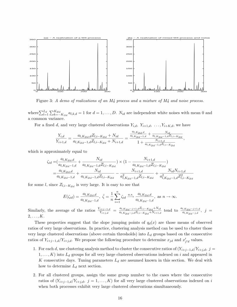
In this section, we address how to determine the values of the points {x1d, x2d, . . . , xmd, d =1, . . . , D}, and {x′1d′ , x′2d′ , . . . , x′m′d′ , d′ = 2, . . . , D}, which are used in estimating parametersin an M4 process of which the parameters Ld, K1ld and K2ld are assumed known. The case ofunknown parameter values of Ld, K1ld and K2ld is addressed in Section 5 with financial applications.In Section 2, we introduced functions bd(x), or qd(x), and showed the slope jumping points of qd(x)are the ratios of coefficients, i.e. al,j+1,d/al,j,d. In real applications, we would not expect the datato follow exactly the model (2.1), because the degenerate features of repeated signature patterns arenot likely to be real phenomena. Nevertheless, our hope is that with large enough Ld, Kild and K2kd,the model will provide a good approximation to the finite-dimensional extreme value distributions.As an example, Figure 3 shows simulated realizations of an M4 process and a mixture of an M4process and a white noise process. Plot (a) is based on

Yi = max(.1Z1,i−1, .4Z1,i, .35Z2,i−1, .15Z2,i), (4.1)

and Plot (b) is based on

Yi = max(.1Z1,i−1, .4Z1,i, .35Z2,i−1, .15Z2,i) + Ni, (4.2)

where Ni ∼ N(0, .1) are i.i.d. Visually, Plots (a) and (b) are very close, but plots of local regions withmagnified scale will show the differences. This phenomenon suggests (4.1) is a good approximationof (4.2). In Section 2, we illustrated that the blowups were caused by the very large Zli values.Consider now the following model:

Yid = max1≤l≤Ld

max−K1ld≤k≤K2ld

al,k,dZl,i−k + Nid, −∞ < i < ∞, d = 1, . . . , D, (4.3)

15

0 100 200 3000

50

100

150

200

250

300

350(a) − A realization of a M4 process

0 100 200 3000

50

100

150

200

250

300

350(b) − A realization of mixed M4 process and noise

Figure 3: A demo of realizations of an M4 process and a mixture of M4 and noise process.

where∑Ld

l=1

∑K2ldk=−K1ld

al,k,d = 1 for d = 1, . . . , D. Nid are independent white noises with mean 0 anda common variance.

For a fixed d, and very large clustered observations Yi,d, Yi+1,d, . . . , Yi+K,d, we have

Yi,d

Yi+1,d=

al,K2ld,dZl,i−K2ld+ Nid

al,K2ld−1,dZl,i−K2ld+ Ni+1,d

=

al,K2ld,d

al,K2ld−1,d+ Nid

al,K2ld−1,dZl,i−K2ld

1 + Ni+1,d

al,K2ld−1,dZl,i−K2ld

,

which is approximately equal to

ζid =(al,K2ld,d

al,K2ld−1,d+

Nid

al,K2ld−1,dZl,i−K2ld

)× (1− Ni+1,d

al,K2ld−1,dZl,i−K2ld

)

=al,K2ld,d

al,K2ld−1,d+

Nid

al,K2ld−1,dZl,i−K2ld

− Ni+1,d

a2l,K2ld−1,dZl,i−K2ld

+NidNi+1,d

a2l,K2ld−1,dZ

2l,i−K2ld

for some l, since Zl,i−K2ldis very large. It is easy to see that

E(ζid) =al,K2ld,d

al,K2ld−1,d, ζ =

1n

n∑

i=1

ζida.s.−→ al,K2ld,d

al,K2ld−1,d, as n →∞.

Similarly, the average of the ratios Yi+j−1,d

Yi+j,d=

al,K2ld−j+1,dZl,i−K2ld+Nid

al,K2ld−j,dZl,i−K2ld+Ni+1,d

tend toal,K2ld−j+1,d

al,K2ld−j,d, j =

2, . . . , K.These properties suggest that the slope jumping points of qd(x) are those means of observed

ratios of very large observations. In practice, clustering analysis method can be used to cluster thosevery large clustered observations (above certain thresholds) into Ld groups based on the consecutiveratios of Yi+j−1,d/Yi+j,d. We propose the following procedure to determine xjd and x′j′d values.

1. For each d, use clustering analysis method to cluster the consecutive ratios of (Yi+j−1,d/Yi+j,d, j =1, . . . , K) into Ld groups for all very large clustered observations indexed on i and appeared inK consecutive days. Tuning parameters Ld are assumed known in this section. We deal withhow to determine Ld next section.

2. For all clustered groups, assign the same group number to the cases where the consecutiveratios of (Yi+j−1,d/Yi+j,d, j = 1, . . . , K) for all very large clustered observations indexed on i

when both processes exhibit very large clustered observations simultaneously.

16

3. Within each group, take the averages of the ratios as slope jumping points. Between any twoadjacent jumping points, arbitrarily choose two points as xjd values. For example, supposer1, r2 are two adjacent ratios, then a natural choice would be xjd = r1 + .25(r2− r1), xj+1,d =r1 + .75(r2 − r1).

4. The choices of x′j′d can be done from averaging the ratios of Yi1/Yid within the same groupnumbers obtained in Step 2 between two processes. Then x′j′d can take the middle values oftwo adjacent ratios or take two values between two adjacent ratios like the previous step.

5. After choosing xjd and x′j′d values, use them to estimate al,k,d based on bd(x) and b1d(x)functions.

Remark 8 In Step 1, we may need to cluster those very large clustered observations into more thanLd groups since outliers may exist and cause the clustering method fail to recognize the true patterns.In our example, we cluster those observations into Ld +3 groups. We discard the 3 groups which arevery small proportions among all those very large clustered observations.

Remark 9 In Step 3 and 4, theoretically, we can choose as many points of xjd and x′j′d as possible,but it is not realistic due to the intensive computation and the complexity of inferences. The goal isto choose moderate number of points such that the estimated values of parameters are close to trueparameter values.

Let us consider a bivariate process and implement the procedures discussed so far. Suppose

Yid = max1≤l≤3

max−1≤k≤1

al,k,dZl,i−k + Nid, −∞ < i < ∞, d = 1, 2, (4.4)

where each M4 process has three signature patterns and moving range order of 3, the noises Nid ∼N(0, .1). The coefficients are listed in Table 1.

The total number of parameters in the M4 process in (4.4) are 18. There is a nuisance parameterthat is the variance of Nid. We do not need to estimate the nuisance parameter in order to estimatethe values of M4 model parameters. We first generate data by simulating these bivariate processes,then based on the simulated data we re-estimate all coefficients simultaneously and compute theirasymptotic covariance matrix. Table 1 is obtained using simulated data with a sample size of 10,000.The xjd and x′j′d values are determined using the procedure described earlier. We use Monte Carlomethod to find best estimations of al,k,ds. For all l, k, d, we simulate 5000 vector values of al,k,ds fromwhich the ratios al,k+1,d/al,k,d and al,k,1/al,k,d (d > 1), are falling in the regions determined by xjd,x′j′d computed in Steps 3 and 4. We keep the vector whose ratios al,k+1,d/al,k,d, al,k,1/al,k,d have theminimal distance to the estimated ratios also obtained in Steps 3 and 4. Theoretical values of bd(x)and b1d(x) are computed using the kept al,k,d values. We repeat this process 100 times and keepthe vector which gives the minimal distance from the simulated ratios al,k+1,d/al,k,d, al,k,1/al,k,d, andtheoretical values of bd(x) and b1d(x) computed using the kept al,k,d values to the estimated ratiosobtained in Steps 3 and 4 and the estimated functions bd(x) and b1d(x).

In Table 1, the estimated values of all cases are very close to the true parameter values. Theestimated standard deviations are very small. These results have shown the efficiency of the proposedestimating procedures.

17

Parameter True Estimated Standard Parameter True Estimated Standardvalue value deviation value value deviation

a1,−1,1 .1500 .0945 .0438 a1,−1,2 .0700 .0387 .0293a1,0,1 .2000 .1258 .0332 a1,0,2 .0400 .0234 .0106a1,1,1 .0200 .0106 .0402 a1,1,2 .0300 .0174 .0137a2,−1,1 .0500 .0575 .0556 a2,−1,2 .1000 .0970 .0256a2,0,1 .1000 .1141 .0529 a2,0,2 .1300 .1261 .0336a2,1,1 .0300 .0290 .0465 a2,1,2 .1700 .1726 .0476a3,−1,1 .1600 .2101 .0473 a3,−1,2 .1100 .1300 .0328a3,0,1 .1700 .2139 .0613 a3,0,2 .1200 .1367 .0335a3,1,1 .1200 .1445 .0574 a3,1,2 .2300 .2580 .0608

Table 1: Simulation results for model (4.4). xj1 =(0.0811, 0.1561, 0.2522, 0.4023, 0.6065, 0.7970,0.9737, 1.1299, 1.2656, 1.4998, 1.8323, 2.1984). xj2 =(0.4276, 0.6243, 0.7325, 0.8630, 1.0157,1.1438, 1.2474, 1.3013, 1.3057, 1.4595, 1.7630, 2.1062). x′j′ =(0.1323, 0.2571, 0.4187, 0.5051,0.5163, 0.5627, 0.6442, 0.7058, 0.7475, 0.9301, 1.2537, 1.4254, 1.4452, 1.6269, 1.9706, 2.8595,4.2938, 5.5120). Standard deviations are computed by applying Theorem 3.5.

5 Modeling jumps in returns of financial assets as M4 processes

As mentioned earlier, our goal is to model multivariate financial time series, particularly jumps inreturns, as M4 processes. Figure 4 are time series plots of three stock returns, i.e. returns fromGeneral Electric Co., CITI Group, and Pfizer Inc. They are selected from top 10 NYSE volumeleaders on day March 12, 2001. The starting date is January 4, 1982. One can see there are extremalobserved values in each sequence and there are jumps in volatilities and returns. Since the marginaldistribution of the original data are not unit Frechet, data transformations are needed in order toapply M4 process modeling. Since local standardization of data may remove the jumps in volatilitiesfrom the data and distributional transformation of data can give unit Frechet margins, they areapplied in this data analysis.

5.1 Data transformation

Research has shown that the GARCH (generalized autoregressive conditional heteroscedasticity)model, proposed by Bollerslev (1986), has been quite successful to the use of fitting financial timeseries data. Mikosch (2003) gives a very thorough study of GARCH modeling of dependence andtails of financial time series. Here we do not study GARCH modeling, but use it as a tool to modelvolatilities. GARCH(1,1) and GARCH(2,2) models have been used to model the volatility in thisanalysis. The estimated standard deviations are drawn in Figure 5. The original data sets are thendivided by the estimated conditional standard deviation and three new time series, standardized timeseries – GARCH residuals – are obtained. Study of GARCH residual has drawn a major attentionrecently, for example McNeil and Frey (2000), Engle (2002), among others. In this paper, we furtherstudy the tail dependencies between and within multivariate financial time series, especially, theGARCH residuals. Figure 6 shows standardized time series. Visually they look stationary.

18

01/04/82 09/30/84 06/27/87 03/23/90 12/17/92 09/13/95 06/09/98 03/05/01−0.2

−0.15

−0.1

−0.05

0

0.05

0.1

0.15

0.2

GE

Neg L

og Re

turn

Negative Daily Return 1982−2001

01/04/82 09/30/84 06/27/87 03/23/90 12/17/92 09/13/95 06/09/98 03/05/01−0.2

−0.15

−0.1

−0.05

0

0.05

0.1

0.15

0.2

CITI

Neg L

og Re

turn

01/04/82 09/30/84 06/27/87 03/23/90 12/17/92 09/13/95 06/09/98 03/05/01−0.2

−0.15

−0.1

−0.05

0

0.05

0.1

0.15

0.2

PFIZER

Neg L

og Re

turn

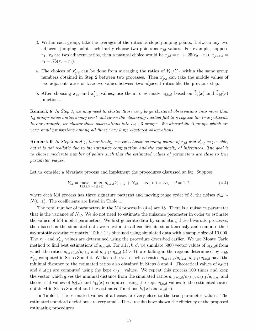
Figure 4: Negative daily returns. The top plot is for General Electric Co., the middle plot is for CITIGroup, and the bottom plot is for Pfizer. These figures show that there are extremal observations andthe highest drops happened in the same day in all three time series, i.e. October 19, 1987, the dateof the Wall Street crash.

0 500 1000 1500 2000 2500 3000 3500 4000 4500 50000

0.01

0.02

0.03

0.04

0.05

0.06Estimated Conditional Standard Deviation Using GARCH(1,1)

GE data

0 500 1000 1500 2000 2500 3000 3500 4000 4500 50000.01

0.02

0.03

0.04

0.05

0.06

0.07

0.08

0.09

CITI Bank data

0 500 1000 1500 2000 2500 3000 3500 4000 4500 50000.01

0.02

0.03

0.04

0.05

0.06

0.07

Pfizer data

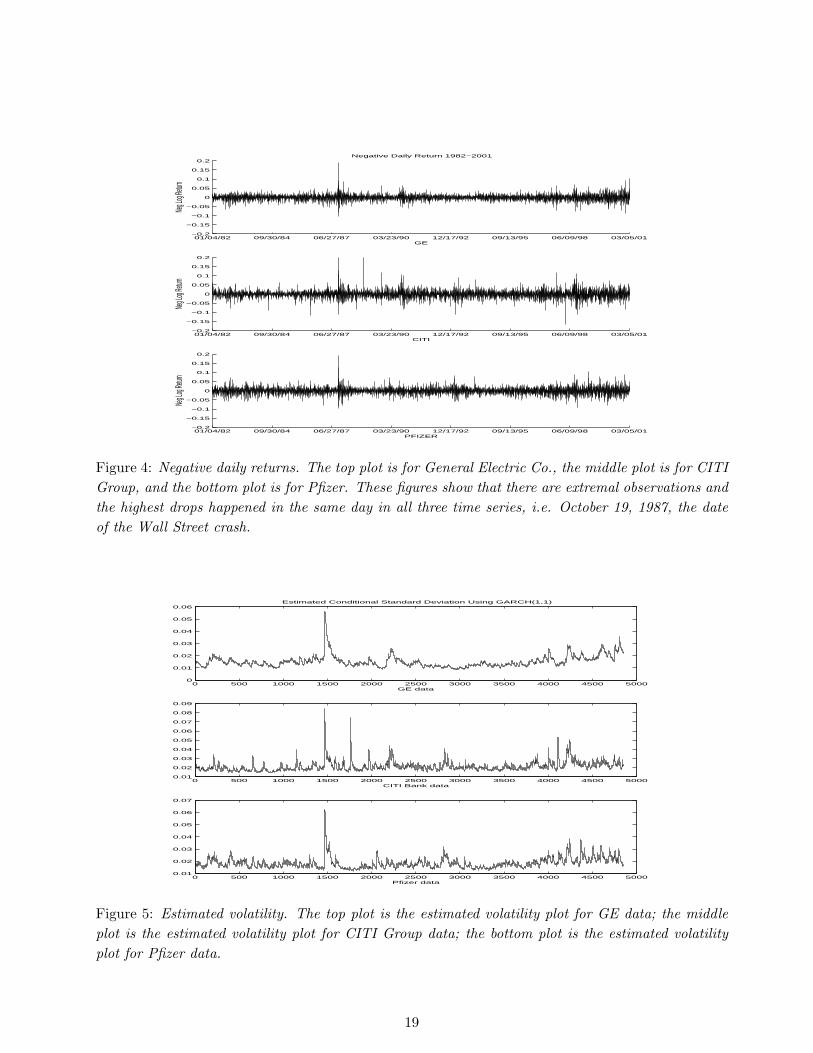
Figure 5: Estimated volatility. The top plot is the estimated volatility plot for GE data; the middleplot is the estimated volatility plot for CITI Group data; the bottom plot is the estimated volatilityplot for Pfizer data.

19

01/04/82 09/30/84 06/27/87 03/23/90 12/17/92 09/13/95 06/09/98 03/05/01−10

−5

0

5

10

GE

Neg L

og Re

turn

Negative Daily Return Divided by Estimated Standard Deviation, 1982−2001

01/04/82 09/30/84 06/27/87 03/23/90 12/17/92 09/13/95 06/09/98 03/05/01−10

−5

0

5

10

CITI

Neg L

og Re

turn

01/04/82 09/30/84 06/27/87 03/23/90 12/17/92 09/13/95 06/09/98 03/05/01−10

−5

0

5

10

PFIZER

Neg L

og Re

turn

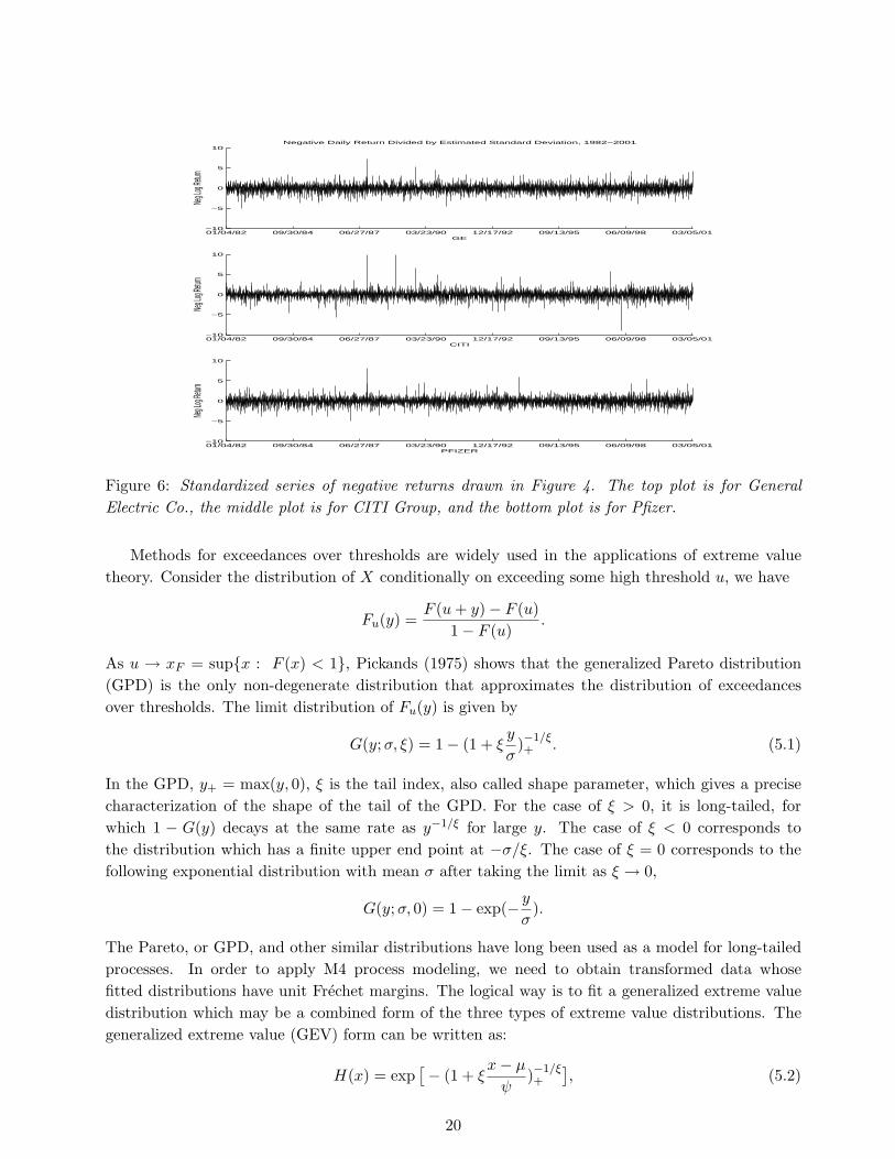
Figure 6: Standardized series of negative returns drawn in Figure 4. The top plot is for GeneralElectric Co., the middle plot is for CITI Group, and the bottom plot is for Pfizer.

Methods for exceedances over thresholds are widely used in the applications of extreme valuetheory. Consider the distribution of X conditionally on exceeding some high threshold u, we have

Fu(y) =F (u + y)− F (u)

1− F (u).

As u → xF = sup{x : F (x) < 1}, Pickands (1975) shows that the generalized Pareto distribution(GPD) is the only non-degenerate distribution that approximates the distribution of exceedancesover thresholds. The limit distribution of Fu(y) is given by

G(y;σ, ξ) = 1− (1 + ξy

σ)−1/ξ+ . (5.1)

In the GPD, y+ = max(y, 0), ξ is the tail index, also called shape parameter, which gives a precisecharacterization of the shape of the tail of the GPD. For the case of ξ > 0, it is long-tailed, forwhich 1 − G(y) decays at the same rate as y−1/ξ for large y. The case of ξ < 0 corresponds tothe distribution which has a finite upper end point at −σ/ξ. The case of ξ = 0 corresponds to thefollowing exponential distribution with mean σ after taking the limit as ξ → 0,

G(y; σ, 0) = 1− exp(− y

σ).

The Pareto, or GPD, and other similar distributions have long been used as a model for long-tailedprocesses. In order to apply M4 process modeling, we need to obtain transformed data whosefitted distributions have unit Frechet margins. The logical way is to fit a generalized extreme valuedistribution which may be a combined form of the three types of extreme value distributions. Thegeneralized extreme value (GEV) form can be written as:

H(x) = exp[− (1 + ξ

x− µ

ψ)−1/ξ+

], (5.2)

20

where µ is a location parameter, ψ > 0 is a scale parameter, and ξ is a shape parameter. Pickands(1975) establishes the rigorous connection of the GPD with the GEV. He shows that for any given F ,a GPD approximation arises from (5.1), if and only if the classical extreme value limits (5.2) holdswith the same shape parameter ξ in (5.1). Thus there is a close parallel between limit results forsample maxima and limit results for exceedances over threshold, which is quite extensively exploitedin modern statistical methods for extremes.

Using the connection between the GPD and the GEV, we can fit the GPD to the exceedancesover thresholds and then get the GEV for the sample maxima, but there are often many situationsin which a GPD fitting may not be appropriate. In practice, the mean excess plot, Z-plot and W -plot can tell whether the extreme value distribution fitting to those extreme values of the returns isappropriate or not. The mean excess plot is a plot of the mean of all excess values over a thresholdu against u itself. It usually suggests whether a extreme value distribution fitting is appropriate ornot. It is very useful for initial diagnostics and selecting the threshold. The underlying idea behindthe analysis of Z-statistics and W -statistics is the point-process approach to univariate extremevalue modeling due to Smith (1989). According to this viewpoint, the exceedance times and excessvalues of a high threshold are viewed as a two-dimensional point process. If the process is stationaryand satisfies a condition that there are asymptotically no clusters among the high-level exceedances,then its limiting form is non-homogeneous Poisson. Smith and Shively (1995) introduce a number ofdiagnostic devices to examine the fit of the generalized extreme value distributions. These techniqueshave been broadly used in model diagnostics, for example, Tsay (1999), Smith and Goodman (2000).Smith (2003) is an extensive source of model diagnostics. We have applied these graphical diagnostictools to both the original data and standardized data and concluded that extreme value distributionfittings are not appropriate to the original data. The diagnostic results have suggested a good fittingof standardized data. We skip the intermediate steps used to diagnose the data and only report thefinal transformed data since the main purpose of the paper is to illustrate the estimating proceduresof the M4 process. For those steps, we refer to Zhang and Smith (2001), Zhang (2002), and Smith(2003).

Since the GEV is easier to handle for transforming to and from the Frechet distribution, it is usedto fit the data above a certain threshold (.02 is used for original data, and 1.2 for standardized datain this study) for each sequence. Considering there are some asymmetric behavior between positivereturns and negative returns, we fit the standardized positive returns and negative returns to GEVseparately. The estimated parameter values of the GEV distributions are summarized in Table 2 (forstandardized negative returns), and Table 3 (standardized positive returns). From these two tables,we see that all negative returns are long-tailed, but not all positive returns are long-tailed since notall estimated shape parameter values are positive.

The data are then transformed into the Frechet scale from fitted GEV function. We combinethe transformed data into three new time series which are standardized and transformed absolutereturns. The transformed data are plotted in Figure 7. The final transformed data are the base ofthe M4 process modeling.

21

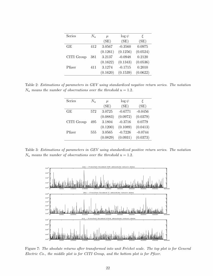
Series Nu µ log ψ ξ

(SE) (SE) (SE)GE 412 3.0567 -0.3560 0.0975

(0.1261) (0.1256) (0.0524)CITI Group 381 3.2137 -0.0948 0.2120

(0.1622) (0.1343) (0.0536)Pfizer 411 3.1274 -0.1715 0.2010

(0.1620) (0.1539) (0.0622)

Table 2: Estimations of parameters in GEV using standardized negative return series. The notationNu means the number of observations over the threshold u = 1.2.

Series Nu µ log ψ ξ

(SE) (SE) (SE)GE 572 3.0725 -0.6771 -0.0456

(0.0883) (0.0972) (0.0379)CITI Group 495 3.1804 -0.3716 0.0779

(0.1200) (0.1089) (0.0413)Pfizer 555 3.0565 -0.7226 -0.0744

(0.0829) (0.0931) (0.0373)

Table 3: Estimations of parameters in GEV using standardized positive return series. The notationNu means the number of observations over the threshold u = 1.2.

0 500 1000 1500 2000 2500 3000 3500 4000 4500 500010

0

101

102

103

104

(a) − Frechet Scaled GE absolute return data

0 500 1000 1500 2000 2500 3000 3500 4000 4500 500010

0

101

102

103

104

105

(b) − Frechet Scaled C absolute return data

0 500 1000 1500 2000 2500 3000 3500 4000 4500 500010

0

101

102

103

104

(c) − Frechet Scaled PFE absolute return data

Figure 7: The absolute returns after transformed into unit Frechet scale. The top plot is for GeneralElectric Co., the middle plot is for CITI Group, and the bottom plot is for Pfizer.

22

5.2 Model selection and the determination of tuning parameters Ld, K1ld, K2ld

An M4 process has double indexes – one for signature patterns and one for moving ranges. Therefore,in order to apply M4 modeling we need to determine the order of moving range and the numberof signature patterns. The order of moving range can be regarded as a measure of asymptoticdependence – or extremal dependence, tail dependence – among a sequence of random variables,while the number of signature patterns tells how many clustered extremal moving patterns existingin each process. The concept – which will be reviewed next – of asymptotic dependencies betweenrandom variables is used in determining the orders of moving ranges in this data analysis.

Sibuya (1960) introduces the concept of the asymptotic independence of a bivariate randomvector with identical marginal distribution. De Haan and Resnick (1977) extend it to the case ofmultivariate random variables. The definitions of asymptotic independence (or tail independence)and asymptotic dependence (or tail dependence) for a bivariate random vector are stated below.

Definition 5.1 Suppose random variables Υ1 and Υ2 are identically distributed with xF = sup{x ∈R : Pr(Υ1 ≤ x) < 1}. The following quantity

λ = limu→xF

Pr(Υ1 > u|Υ2 > u) (5.3)

is called the bivariate tail dependence index, or the tail dependence index, between Υ1 and Υ2. Itquantifies the amount of dependence of the bivariate upper tails of Υ1 and Υ2. If λ > 0, then Υ1

and Υ2 are called tail dependent, otherwise the two random variables are called tail independent.

Zhang (2003) extends this definition to lag-k tail dependencies among a sequence of random variables.

Definition 5.2 A sequence of sample {Υ1, Υ2, . . . , Υn} is called lag-k tail dependent if

λk = limu→xF

Pr(Υ1 > u|Υk+1 > u) > 0, limu→xF

Pr(Υ1 > u|Υk+j > u) = 0, j > 1 (5.4)

where xF = sup{x ∈ R : Pr(Υ1 ≤ x) < 1}. λk is called the lag-k tail dependence index.

Under Model (2.1), it is easy to show that the extremal (tail) dependence index λdd′ between Yid

and Yid′ is:

λdd′ = 2−max(Ld,Ld′ )∑

l=1

1+max(K1ld,K1ld′ )∑

m=1−max(K2ld,K2ld′ )

max{al,1−m,d, al,1−m,d′

},

and {Yid} is lag-k – where k = max1≤l≤Ld(K1ld + K2ld) – tail dependent and its index is:

lλdk = 2−Ld∑

l=1

1+k+K1ld∑

m=1−K2ld

max{al,1−m,d, al,1+k−m,d

}.

Our model selection is based on whether the data would suggest λdd′ > 0 and lλdk > 0. Thisturns out to be a hypothesis testing problem. Having derived the asymptotic joint distributionsfor all parameter estimators, we may be able to construct confidence intervals for tail dependenceindexes, at least to construct Monte Carlo confidence intervals. Then a test can be performedbased on constructed confidence intervals. An alternative way to perform test is to use the gamma

23

Range of days 1 2 3 4 5 6GE 327 51 16 2 2 1

(402.8) (41.6) (4.3) (.4) (.05) (.005)C 416 30

(387.1) (38.0)PFE 383 40 4

(386.1) (37.8) (3.7)

Table 4: Counts of days that the absolute returns are over a threshold value in consecutive days.All counts are mutually exclusive. Numbers in parenthesis are computed from a Bernoulli processassumption.

test developed in Zhang (2003). Since our focus here is on the estimation, it is preferred to usea practically simple approach to determine the orders of moving ranges, the numbers of signaturepatterns, and the dependence structure. We study the empirical estimates of tail dependence indexesbetween random variables using empirical counts.

Based on the properties that an M4 process appears to have clustered observations when anextreme observation occurs, we check those observed values which are larger than a certain threshold.Among the observations empirical counts can tell both the moving range order and the cross-sectionaldependence range. We look at the counts of paired absolute daily returns on the unit Frechet scalein different ways. We count the days when two different stock absolute returns both were over acertain threshold. We count the days when the absolute returns of a single stock were over a certainthreshold on two or more consecutive days. When a threshold value of 2 is used, we find that themaximal range of consecutive days from which the jumps in returns are over the threshold valueare 6, 2, 3 days for GE, C, and PFE respectively. While the empirical estimates of tail dependenceindexes can be computed by the division of counts for each range over the total number of days thatexceedances occur, we simply use counts here. We summarize the counts information within eachrange in Table 4.

In Table 4, apparently, tail independence assumptions for GE and C data are violated. For GEdata, the total number of single jumps are much less than the expected total number (in parenthesis).This phenomenon suggests that there are tail dependencies within sequences as also suggested byother numbers from different ranges of days. For C data, we observe that the total number of singlejumps are larger than the expected total number, while the total number of jumps in two consecutivedays are less than the expected total number. This phenomenon suggests that it is likely we wouldobserve more jumps in consecutive days in a different time period. For PFE data, we observe asimilar phenomenon as in GE data while the observed numbers are more close to the expected totalnumbers.

It might be safe to say that Table 4 suggests that a model of time dependence range of order3 and at least 3 signature patterns for GE data; a model of time dependence range of order 2 and2 signature patterns for C data; and a model of time dependence range of order 2 and at least 2signature patterns for PFE data. Some of these patterns have order of 3, corresponding to jumpsthat happened in three consecutive days, some of these patterns have order of 2, corresponding tojumps that happened in two consecutive days, and one has order of 1, which corresponds to a single

24

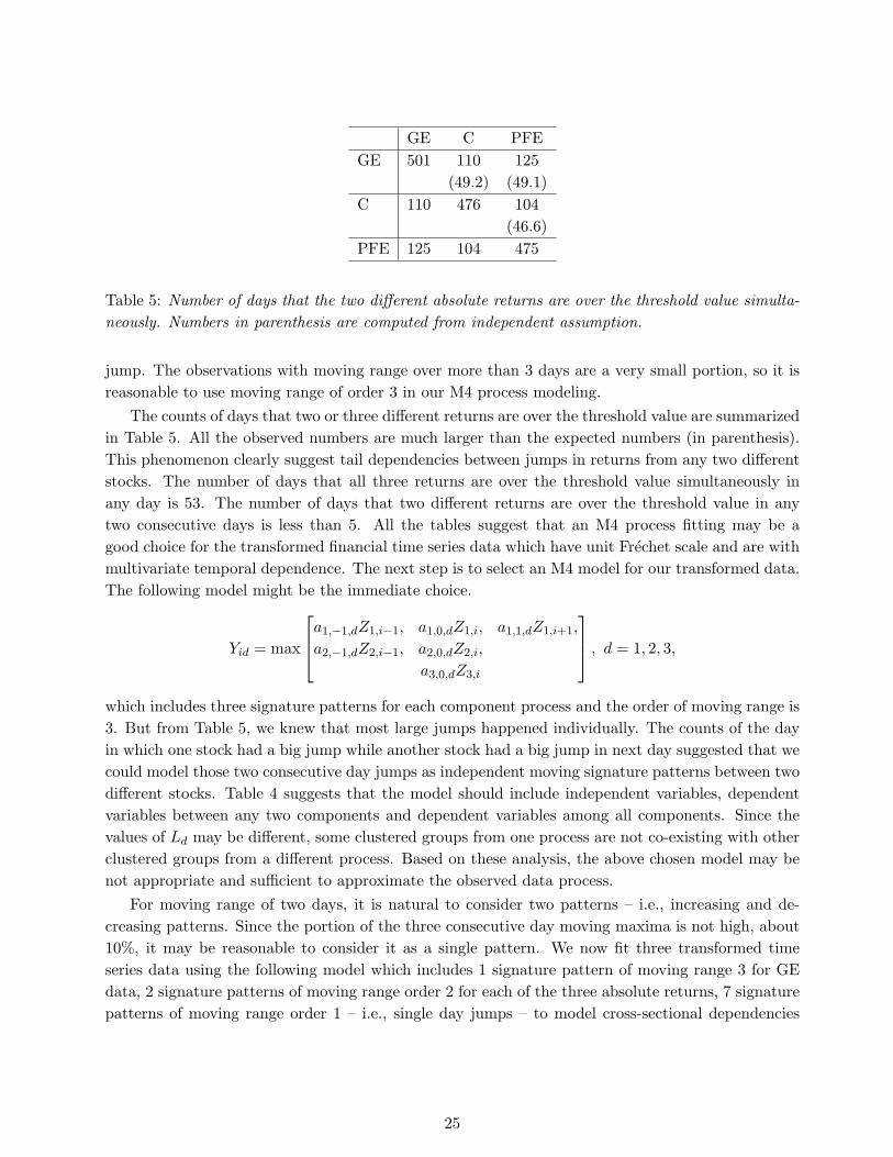
GE C PFEGE 501 110 125

(49.2) (49.1)C 110 476 104

(46.6)PFE 125 104 475

Table 5: Number of days that the two different absolute returns are over the threshold value simulta-neously. Numbers in parenthesis are computed from independent assumption.

jump. The observations with moving range over more than 3 days are a very small portion, so it isreasonable to use moving range of order 3 in our M4 process modeling.

The counts of days that two or three different returns are over the threshold value are summarizedin Table 5. All the observed numbers are much larger than the expected numbers (in parenthesis).This phenomenon clearly suggest tail dependencies between jumps in returns from any two differentstocks. The number of days that all three returns are over the threshold value simultaneously inany day is 53. The number of days that two different returns are over the threshold value in anytwo consecutive days is less than 5. All the tables suggest that an M4 process fitting may be agood choice for the transformed financial time series data which have unit Frechet scale and are withmultivariate temporal dependence. The next step is to select an M4 model for our transformed data.The following model might be the immediate choice.

Yid = max

a1,−1,dZ1,i−1, a1,0,dZ1,i, a1,1,dZ1,i+1,

a2,−1,dZ2,i−1, a2,0,dZ2,i,

a3,0,dZ3,i

, d = 1, 2, 3,

which includes three signature patterns for each component process and the order of moving range is3. But from Table 5, we knew that most large jumps happened individually. The counts of the dayin which one stock had a big jump while another stock had a big jump in next day suggested that wecould model those two consecutive day jumps as independent moving signature patterns between twodifferent stocks. Table 4 suggests that the model should include independent variables, dependentvariables between any two components and dependent variables among all components. Since thevalues of Ld may be different, some clustered groups from one process are not co-existing with otherclustered groups from a different process. Based on these analysis, the above chosen model may benot appropriate and sufficient to approximate the observed data process.

For moving range of two days, it is natural to consider two patterns – i.e., increasing and de-creasing patterns. Since the portion of the three consecutive day moving maxima is not high, about10%, it may be reasonable to consider it as a single pattern. We now fit three transformed timeseries data using the following model which includes 1 signature pattern of moving range 3 for GEdata, 2 signature patterns of moving range order 2 for each of the three absolute returns, 7 signaturepatterns of moving range order 1 – i.e., single day jumps – to model cross-sectional dependencies

25

between component absolute returns.

Yid = max

a1,−1,dZ1,i−1, a1,0,dZ1,i, a1,1,dZ1,i+1,

a2,−1,dZ2,i−1, a2,0,dZ2,i,...

...a7,−1,dZ7,i−1, a7,0,dZ7,i,

a8,0,dZ8,i,...

a14,0,dZ14,i

, d = 1, 2, 3, (5.5)

where al,k,d = 0 for {l = 1, 2, 3, 8, d = 2, 3}; {l = 4, 5, 9, d = 1, 3}; {l = 6, 7, 10, d = 1, 2};{l = 12, d = 3}; {l = 13, d = 2}; {l = 14, d = 1}. This model is still a simple one. Morecomplicated structures can be adopted. But we restrict our attention to a relatively simple modelsince the ideas can be easily extended to more detailed considerations.

5.3 Parameter estimation

Before we proceed to estimate all parameters in Model (5.5), we give the following remark whichmay be very useful when we perform numerical computations of point estimation of the parameters.

Remark 10 From Propositions 2.2, 2.3, 2.4, Lemma 3.4, and (3.8), we know that if the process isone-dimensional, then bd(x) determines all parameter estimates; if the process is a high dimensional,then bdd′s match all signature patterns between any two individual processes. For some observed pro-cesses, those matches can be done by examining observed moving signature patterns in the sequenceswithout involving any bdd′(x) functions.

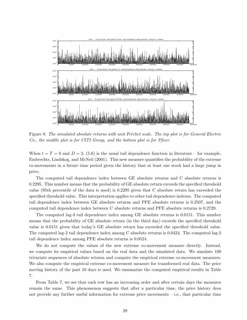
Considering the special structure of (5.5), we estimate parameter values by using bd(x) only. Theestimation is processed using the methods described in Section 4. Based on Remark 1, the estimatedproportions of each signature patterns are used as constraints. The estimated results are summarizedin 6. Simulated triple absolute return time series are plotted in Figure 8.

5.4 Statistical inference

Having established the statistical model for the data, the next step is to make statistical inference.Here we are particularly interested in computing tail dependence indexes defined earlier and a newextreme co-movement measure which is:

λ(t, T ) = limu↗xF

Pr{ξ(t, T,u) ≥ 2|ξ(0, t,u) ≥ 1} (5.6)

where xF is the right end point of the distribution function F , ξ(s, t,u) is a random variable corre-sponds to the maxima of maximal numbers of risk factors which have values beyond certain thresholdover a time period (s, t), i.e.

ξ(s, t,u) = maxs≤i≤t

D∑

d=1

I(Yid>ud). (5.7)

26

Table 6: Estimations of Parameters in model (5.5). The values in parentheses are standard errors.

Signature General Electric CITI Group Pfizerl al,−1,1 al,0,1 al,1,1 al,−1,2 al,0,2 al,−1,3 al,0,3

1 0.0176 0.0262 0.0543(0.0467) (0.0732) (0.1840)

2 0.0517 0.0391(0.0744) (0.0520)

3 0.0247 0.0816(0.1538) (0.5599)

4 0.0220 0.0200(0.0799) (0.0647)

5 0.0264 0.0492(0.0877) (0.2145)

6 0.0540 0.0372(0.0872) (0.0732)

7 0.0254 0.0586(0.0944) (0.2812)

8 0.0746 0.0982 0.0920(0.0439) (0.0208) (0.0271)

9 0.1547 0.2039(0.0911) (0.0431)

10 0.1758 0.2170(0.1035) (0.0638)

11 0.1928 0.1806(0.0408) (0.0531)

12 0.2996(0.1764)

13 0.3874(0.0819)

14 0.3351(0.0985)

27

0 500 1000 1500 2000 2500 3000 3500 4000 4500 500010

0

101

102

103

104

(a) − Frechet Scaled GE simulated absolute return data

0 500 1000 1500 2000 2500 3000 3500 4000 4500 500010

0

101

102

103

104

(b) − Frechet Scaled C simulated absolute return data

0 500 1000 1500 2000 2500 3000 3500 4000 4500 500010

0

101

102

103

104

(c) − Frechet Scaled PFE simulated absolute return data

Figure 8: The simulated absolute returns with unit Frechet scale. The top plot is for General ElectricCo., the middle plot is for CITI Group, and the bottom plot is for Pfizer.

When t = T = 0 and D = 2, (5.6) is the usual tail dependence function in literature – for example,Embrechts, Lindskog, and McNeil (2001). This new measure quantifies the probability of the extremeco-movements in a future time period given the history that at least one stock had a large jump inprice.

The computed tail dependence index between GE absolute returns and C absolute returns is0.2295. This number means that the probability of GE absolute return exceeds the specified thresholdvalue (95th percentile of the data is used) is 0.2295 given that C absolute return has exceeded thespecified threshold value. This interpretation applies to other tail dependence indexes. The computedtail dependence index between GE absolute returns and PFE absolute returns is 0.2507, and thecomputed tail dependence index between C absolute returns and PFE absolute returns is 0.2729.

The computed lag-3 tail dependence index among GE absolute returns is 0.0151. This numbermeans that the probability of GE absolute return (in the third day) exceeds the specified thresholdvalue is 0.0151 given that today’s GE absolute return has exceeded the specified threshold value.The computed lag-2 tail dependence index among C absolute returns is 0.0424. The computed lag-2tail dependence index among PFE absolute returns is 0.0524.

We do not compute the values of the new extreme co-movement measure directly. Instead,we compute its empirical values based on the real data and the simulated data. We simulate 100trivariate sequences of absolute returns and compute the empirical extreme co-movement measures.We also compute the empirical extreme co-movement measure for transformed real data. The pricemoving history of the past 10 days is used. We summarize the computed empirical results in Table7.

From Table 7, we see that each row has an increasing order and after certain days the measuresremain the same. This phenomenon suggests that after a particular time, the price history doesnot provide any further useful information for extreme price movements – i.e., that particular time

28

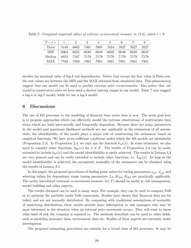
Table 7: Computed empirical values of extreme co-movement measure in (5.6), where t = 9.

T − t = 1 2 3 4 5 6 7 8Data .5149 .6862 .7461 .7605 .7624 .7627 .7627 .7627MIN .6364 .6635 .6648 .6648 .6648 .6648 .6648 .6648

Median .6853 .7167 .7179 .7179 .7179 .7179 .7179 .7179MAX .7532 .7850 .7861 .7861 .7861 .7861 .7861 .7861

decides the maximal value of lag-k tail dependencies. Notice that except the first value in Data row,the rest values are between the MIN and the MAX obtained from simulated data. This phenomenonsuggest that our model can be used to predict extreme price co-movements. Also notice that ourmodel is conservative since we have used a shorter moving ranges in our model. Table 7 may suggesta lag-4 or lag-5 model, while we use a lag-3 model.

6 Discussions

The use of M4 processes to the modeling of financial time series data is new. The main goal hereis to propose approaches which can efficiently model the extreme observations of multivariate timeseries which are both inter-serially and temporally dependent. Because there are many parametersin the model and maximum likelihood methods are not applicable in the estimation of all param-eters, the identifiability of the model plays a major role of constructing the estimators based onempirical functions. We have given sufficient conditions under which the M4 models are identifiable(Proposition 2.4). In Proposition 2.4, we only use the function b1d′(x). In some situations, we alsoneed to consider other functions, bdd′(x) for d 6= d′. The results of Proposition 2.4 can be easilyextended to include bdd′(x) and the model identifiability is easily achieved. The results in Lemma 3.4are very general and can be easily extended to include other functions, i.e. bdd′(x). As long as themodel identifiability is achieved, the asymptotic normality of the estimators can be obtained usingthe results of Lemma 3.4.

In this paper, the proposed procedures of finding point values for tuning parameters xjd, x′j′d′ andselecting values for dependence range tuning parameters Ld, K1ld, K2ld are practically applicable.The newly introduced extremal co-movement measure λ(t, T ) should be useful in risk management,model building and other aspects.

The results obtained can be used in many ways. For example, they can be used to compute VaRor to optimize the portfolio under VaR constraints. Studies have shown that financial data are fattailed, and are not normally distributed. By comparing with traditional assumptions of normalityof underlying distribution, these results provide more information to risk managers who may bemost interested in the situation when an extreme price movement occurs. They will want to knowwhat kind of risk the company is exposed to. The methods described can be used to other fields,such as modeling insurance data, environment data etc. Studies of these aspects are currently underinvestigation.

The proposed estimating procedures are suitable for a broad class of M4 processes. It may be

29

possible to propose some variants of proposed estimators and to reduce the conditions imposed onthe parameters.

7 Technical arguments

Proof of Proposition 2.2. Since all the ratios are different and are points at which qd(x) changesslopes or q′d(x) has jumps. So based on the jump points of qd(x), the ratios of al,j+1,d

al,j,dare uniquely

determined. Let’s now rewrite qd(x) as

qd(x) =Ld∑

l=1

xbld

2+K1ld∑

m=1−K2ld

max(cl,1−m,d,

cl,2−m,d

x

). (7.1)

where∑j

cl,j,d = 1 for each l and all cl,j,d are uniquely determine by the ratios which are the slope

change points of qd(x).Suppose now qd(x) has a different representation, say

qd(x) =Ld∑

l=1

xb′ld2+K1ld∑

m=1−K2ld

max(cl,1−m,d,

cl,2−m,d

x

)(7.2)

then

Ld∑

l=1

(bld − b′ld)2+K1ld∑

m=1−K2ld

max(cl,1−m,d,

cl,2−m,d

x

)= 0 (7.3)

for all x.Suppose we have chosen x1, x2, . . . , xLd−1 and formed the matrix

∆d =

2+K1ld∑m=1−K2ld

max(c1,1−m,d,c1,2−m,d

x1) · · ·

2+K1ld∑m=1−K2ld

max(cLd,1−m,d,cLd,2−m,d

x1)

.... . .

...2+K1ld∑

m=1−K2ld

max(c1,1−m,d,c1,2−m,d

xL−1) · · ·

2+K1ld∑m=1−K2ld

max(cLd,1−m,d,cLd,2−m,d

xL−1)

1 · · · 1

and set

2+K1ld∑m=1−K2ld

max(c1,1−m,d,c1,2−m,d

x1) · · ·

2+K1ld∑m=1−K2ld

max(cLd,1−m,d,cLd,2−m,d

x1)

.... . .

...2+K1ld∑

m=1−K2ld

max(c1,1−m,d,c1,2−m,d

xL−1) · · ·

2+K1ld∑m=1−K2ld

max(cLd,1−m,d,cLd,2−m,d

xL−1)

1 · · · 1

b1d − b′1d......

bLdd − b′Ldd

= 0.

|∆d| is the determinant of the system of linear equations. Assume now the Ld determinants of the(Ld−1)×(Ld−1) matrices formed from the bottom Ld−1 rows are not all zero. Since cl,k,d are known

30

and∑2+K1ld

m=1−K2ldcl,i−m,d = 1, i = 1, 2, then there exist xmin and xmax such that when x1 < xmin or

x1 > xmax, all elements of first row in ∆d are 1x1

or 1 respectively. This will give two constant rowsin |∆d|, so when x1 < xmin or x1 > xmax, we have |∆d| = 0. When x1 varies in [xmin, xmax], denoting∆d by ∆d(x1), then

|∆d(x1)| = 1x1

∑ci,j,d|∆d|1j +

∑ci′,j′,d|∆d|1j′ (7.4)

where |∆d|1j 6= 0, |∆d|1j′ 6= 0 are the (1, j) or (1, j′) minors of ∆d. Both summations in the righthand side of (7.4) are over all non-zero minors of the first row of ∆d and the corresponding ci,j,d

x1

or ci′,j′,d. If |∆d(x1)| = 0, by varying x1 in [xmin, xmax], at some point x, some 1x1

ci,j,d|∆d|1j of thesummation 1

x1

∑ci,j,d|∆d|1j change to ci′,j′,d|∆d|1j′ and add to

∑ci′,j′,d|∆d|1j′ , or vice versa, and

this change results in |∆d(x)| 6= 0. Hence it cannot be true that |∆d| = 0 for all x1. This argumentcan be applied to lower dimension matrices. On the other hand, we can start from a 2× 2 matrixand extend it to Ld ×Ld matrix such that the determinant is not zero as required. Therefore, thereexist constants x1, , . . . , xLd−1 such that each system of linear equations has a unique solution. Wethen conclude bld = b′ld, for all l. So qd(x) uniquely determine all al,j,d. 2

Proof of Proposition 2.3. By Proposition 2.2, bd(x) and bd′(x) uniquely determine all values ofparameters al,k,d and al,k,d′ respectively. So we can get

(al,−K1ld,d, al,−K1ld+1,d, . . . , al,K2ld,d), l = 1, . . . , Ld

and(al′,−K1ld,d′ , al′,−K1ld+1,d′ , . . . , al′,K2ld,d′), l′ = 1, . . . , Ld.

Since all nonzero existing ratios al,k,d

al,k,d′are distinct, any permutation of index l or index k in the

triple subindex of al,k,d′ will result in different ratios which will be different from the jump points ofqdd′(x), so the jump points of qdd′(x) uniquely determine

( al,−K1ld,d

al,−K1ld,d′,

al,−K1ld+1,d

al,−K1ld+1,d′, · · · ,

al,K2ld,d

al,K2ld,d′

)

for all l. So (2.8) eventually uniquely determine all the true values of all parameters al,k,d and al,k,d′ .The reason why x1, x2, . . . , xm uniquely determine all values of al,k,d and al,k,d′ is because qd(x),

qd′(x) and qdd′(x) are piecewise linear functions which can be uniquely determined by a finite numberof points as long as there are at least two points between any two jump points. 2

Proof of Proposition 2.4. The proof can be done by following the arguments in Proposition 2.3. 2

Proof of Lemma 3.2. Let Υnd = IAjd{Ynd, Yn+1,d} − µjd, then E[Υnd] = 0 and E[Υ12

nd] < ∞ becauseΥnd is bounded. The α-mixing condition is satisfied since Ynd’s are M -dependent. So the conditionsof Proposition 3.1 are satisfied. Then the proof follows after calculating the following values andapplying Proposition 3.1.

Υ21d = IAjd

{Y1d, Y2d} − 2µjdIAjd{Y1d, Y2d}+ µ2

jd,

EΥ21d = µjd − 2µ2

jd + µ2jd = µjd − µ2

jd,

Υ1dΥ1+k,d = (IAjd{Y1d, Y2d} − µjd)(IAjd

{Y1+k,d, Y2+k,d} − µjd)= IAjd

{Y1d, Y2d}IAjd{Y1+k,d, Y2+k,d}

−µjdIAjd{Y1d, Y2d} − µjdIAjd

{Y1+k,d, Y2+k,d}+ µ2jd

31

andE(Υ1dΥ1+k,d) = Pr{Y1d ≤ xjd, Y2d ≤ x′jd, Y1+k,d ≤ xjd, Y2+k,d ≤ x′jd} − µ2

jd.

2

Proof of Lemma 3.3. Let

U1d = (IA1d{Y1d, Y2d} − µ1d, . . . , IAL−1,d

{Y1d, Y2d} − µL−1,d)′,

U1+k,d = (IA1d{Y1+k,d, Y2+k,d} − µ1d, . . . , IAL−1,d

{Y1+k,d, Y2+k,d} − µL−1,d)′,

and α = (α1d, . . . , αL−1,d)′ 6= 0 be an arbitrary vector.Let Υ1d = α′U1d,Υ2d = α′U2d, . . . , then E[Υnd] = 0 and E[Υ12

nd] < ∞. And so Proposition 3.1can apply. We say expectation are applied on all elements if expectation is applied on a randommatrix. But E[Υ2

1d] = α′E[U1dU′1d]α = α′Σα, E[Υ1dΥ1+k,d] = α′E[U1dU

′1+k,d]α = α′Wkdα where

E([IAid{Y1d, Y2d} − µid][IAjd

{Y1d, Y2d} − µjd]) = µi,j,d − µidµjd

E([IAid{Y1d, Y2d} − µid][IAjd

{Y1+k,d, Y2+k,d} − µjd])= Pr{Y1d ≤ xid, Y2d ≤ x′id, Y1+k,d ≤ xjd, Y2+k,d ≤ x′jd} − µidµjd

So the proof is completed by applying the Cramer-Wold device. 2

References

[1] Billingsley, P. (1995) Probability and Measure, 3rd edition, John & Wiley, New York.

[2] Bollerslev, T. (1986) Generalized autoregressive conditional heteroscedasticity. J. Econometrics31, 307-327

[3] Coles, S. G. (2001) An Introduction to Statistical Modeling of Extreme Values, Springer.

[4] Coles, S. G. and Tawn, J. A. (1991) Modeling Extreme Multivariate Events. J. R. Statist. Soc.B, 53,pp. 377-392

[5] Coles, S. G. and Tawn, J. A. (1994) Statistical Methods for Multivariate Extrems: an Applica-tion to Structural Design(with discussion). Appl. Statist. 43, No. 1, pp. 1-48

[6] Davis, R. A. and Resnick, S. I. (1989) Basic Properties and Prediction of Max-ARMA Processes.Adv. Appl. Prob. , 21, 781-803

[7] Davis, R. A. and Resnick, S. I. (1993) Prediction of Stationary Max-Stable Processes. Ann.Appl. Prob. , 3, no 2, 497-525

[8] Deheuvels, P. (1983) Point Processes and Multivariate Extreme Values. Jour. of Multi. Anal.13, pp. 257-272

[9] Embrechts, P., Kluppelberg, C. and Mikosch, T. (1997) Modelling Extremal Events for Insuranceand Finance, Springer

32

[10] Embrechts, P., Lindskog, F. and McNeil, A. (2003) Modelling Dependence with Copulas andApplications to Risk Management In: Handbook of Heavy Tailed Distributions in Finance, ed.S. Rachev, Elsevier, Chapter 8, pp. 329-384

[11] Engle, R. (2002) Dynamic Conditional Correlation - A Simple Class of Multivariate GARCHModels. Journal of Business and Economic Statistics. Vol. 17, No. 5.

[12] Galambos, J. (1987) Asymptotic theory of extreme order statistics, 2nd edition. Krieger, Mal-abar, Florida.

[13] de Haan, L. (1984) A Spectral Representation for Max-Stable Processes. Ann. of Prob. Vol 12,No. 4, 1194-1204

[14] de Haan, L. (1985) Extremes in higher dimensions: the model and some statistics. In Proc. 45thSess. Int. Statist. Inst., paper 26.3. The Hague: International Statistical Institute.

[15] de Haan, L. and Resnick, S. I. (1977) Limit Theory for Multivariate Sample Extremes. Z.Wahrscheinlichkeitstheorie verw. Gebiete, 40, pp.317-337

[16] Hall, P., Peng, L. and Yao. Q. (2002) Moving-maximum models for extrema of time series.Journal of Statistical Planning and Inference, 103, 51 - 63.

[17] Leadbetter, M. R., Lindgren, G. and Rootzen, H. (1983) Extremes and related properties ofrandom sequences and processes. Springer, Berlin.

[18] McNeil, A. and Frey, R. (2000) Estimation of Tail-Related Risk Measures for HeteroscedasticFinancial Time Series: an Extrem Value Approach. Journal of Empirical Finance, 7: 271-300

[19] Mikosch, T., (2003) Modeling Depaendence and Tails of Financial Time Series. In Extreme Valuein Finance, Telecommunications and the Environment, B. Finkenstadt and H. Rootzen, editors,to be published by Chapman and Hall/CRC.

[20] Nandagopalan, S. (1990) Multivariate extremes and the estimation of the extremal index. Ph.D.dissertation, Dept. Of Statistics, University of North Carolina, Chapel Hill.

[21] Nandagopalan, S. (1994) On the multivariate extremal index. J. of Research, National Inst. of

Standards and Technology. 99, 543-550.

[22] Pickands, J. III (1975) Statistical Inference Using Extreme Order Statistics. The Ann. of Statis.

3, No 1, 119-131

[23] Pickands, J. III (1981) Multivariate Extreme Value distributions. Proc. 43rd Session I.S.I.(Buenos Aires), 859-878.

[24] Resnick, S. I. (1987) Extreme Values, Regular Variation, and Point Processes. Springer, NewYork.

[25] Sibuya, M. (1960) Bivariate Extreme Statistics, I. Ann. Inst. Statist. Math, 11, 195-210

[26] Smith, R. L. (1989) Extreme Value Analysis of Environmental time Series: An Application toTrend Detection in Ground-Level Ozone. (with discussion) Statistical Science. 4, No 4, 367-393

33

[27] Smith, R.L. (2003) Statistics of Extremes, with Applications in the Environment, Insurance andFinance. In Extreme Value in Finance, Telecommunications and the Environment, B. Finken-stadt and H. Rootzen, editors, to be published by Chapman and Hall/CRC. Available online athttp://www.stat.unc.edu/postscript/rs/semstatrls.pdf

[28] Smith, R. L. and Goodman, D. J. (2000) Bayesian Risk Ananlysis. Extremes and Integrated

Risk Management, pp. 235-251. (Edited by Paul Embrechts), UBS Warburg.

[29] Smith, R. L., and Shively, T. S. (1995) Point Process Approach to Modeling Trends in Tropo-sphereic Ozone Based on Exceedances of A High Threshold.Atmospheric Environment, 29, No.23, pp.3489-3499

[30] Smith, R. L., and Weissman, I. (1996) Characterization and Estimation of the MultivariateExtremal Index. Manuscript, UNC.

[31] Tsay, R. S. (1999) Extreme Value Analysis of Financial Data. Manuscript, Univ. Of Chicago.

[32] Zhang, Z., (2002) Multivariate Extremes, Max-Stable Process Estimation and Dynamic FinancialModeling, PhD Dissertation, Department of Statistics, University of North Carolina.

[33] Zhang, Z., (2003) Testing Hypothesis of Tail Independence and New Tail Dependence Measures.Manuscript. Submitted.

[34] Zhang, Z. and Smith, R. L. (2001) Modeling financial time series data as moving maximaprocesses. Technical Report, Department of Statistics, University of North Carolina. Submittedto 2001 NBER/NSF time series conference.

[35] Zhang, Z. and Smith, R. L. (2003) Behavior of Multivariate Maxima of Moving Maxima.Manuscript. Submitted.

34