on the formulation of coupled thermoplastic problems with

On the formulation of coupled thermoplasticproblems with phase-change

C. Agelet de Saracibar*, M. Cervera, M. ChiumentiETS Ingenieros de Caminos, Canales y Puertos, International Center for Numerical Methods in Engineering,

Edi®cio C1, Campus Norte, UPC, Gran CapitaÂn s/n, 08034 Barcelona, Spain

Received in final revised form 22 June 1998

Abstract

This paper deals with a numerical formulation for coupled thermoplastic problems includ-ing phase-change phenomena. The ®nal goal is to get an accurate, e�cient and robustnumerical model, allowing the numerical simulation of solidi®cation processes in the metal

casting industry. Some of the current issues addressed in the paper are the following. A fractionalstep method arising from an operator split of the governing di�erential equations has been usedto solve the nonlinear coupled system of equations, leading to a staggered product formulasolution algorithm. Nonlinear stability issues are discussed and isentropic and isothermal

operator splits are formulated. Within the isentropic split, a strong operator split design con-straint is introduced, by requiring that the elastic and plastic entropy, as well as the phase-change induced elastic entropy due to the latent heat, remain ®xed in the mechanical problem.

The formulation of the model has been consistently derived within a thermodynamic frame-work. The constitutive behavior has been de®ned by a thermoelastoplastic free energy func-tion, including a thermal multiphase change contribution. Plastic response has been modeled

by a J2 temperature dependent model, including plastic hardening and thermal softening. Abrief summary of the thermomechanical frictional contact model is included. The numericalmodel has been implemented into the computational Finite Element code COMET developed

by the authors. A numerical assessment of the isentropic and isothermal operator splits,regarding the nonlinear stability behavior, has been performed for weakly and strongly coupledthermomechanical problems. Numerical simulations of solidi®cation processes show the perfor-mance of the computational model developed.# 1999 Elsevier Science Ltd. All rights reserved.

1. Introduction

Numerical solution of coupled problems using staggered algorithms, is an e�-cient procedure in which the original problem is partitioned into several smaller

International Journal of Plasticity 15 (1999) 1±34

0749-6419/99/$Ðsee front matter # 1999 Elsevier Science Ltd. All rights reserved

PII: S0749-6419(98)00055-2

*Corresponding author. Tel.:+34-93-401-6495; fax:+34-93-401-6517; e-mail: [email protected]

sub-problems which are solved sequentially. For thermomechanical problems thestandard approach exploits a natural partitioning of the problem in a mechanicalphase, with the temperature held constant, followed by a thermal phase at ®xedcon®guration. As noted in Simo and Miehe (1992) this class of staggered algorithmsfalls within the class of product formula algorithms arising from an operator split ofthe governing evolution equations into an isothermal step followed by a heat-con-duction step at ®xed con®guration. A recent analysis in Armero and Simo (1992a,b,1993) shows that this isothermal split does not preserve the contractivity property of thecoupled problem of (nonlinear) thermoelasticity leading to staggered schemes that areat best only conditionally stables. Armero and Simo (1992a,b, 1993) proposed analternative operator split, henceforth referred to as the isentropic split, whereby theproblem is partitioned into an isentropic mechanical phase, with total entropy heldconstant, followed by a thermal phase at ®xed con®guration. It was shown by Armeroand Simo (1992a,b, 1993) that such operator split leads to an unconditionally stablestaggered algorithm, which preserves the crucial properties of the coupled problem. Theaim of the paper is to extend the formulation given by Armero and Simo (1992a,b,1993) and Simo (1994) to coupled thermoplastic problems with phase-change, to get anaccurate, e�cient and robust numerical model, allowing the numerical simulation ofsolidi®cation processes in the metal casting industry.The remaining of the paper is as follows. Section 2 deals with the formulation of the

local governing equations of the coupled thermoplastic problem, consistently derivedwithin a thermodynamic framework. An additive split of the strain tensor and theentropy has been assumed. The constitutive behavior has been de®ned by a thermo-elastoplastic free energy function, with temperature dependent material properties.Latent heat associated to the phase-change phenomena has been incorporated to thethermal contribution of the free energy function. Plastic response has been modeled bya J2 temperature dependent model, including nonlinear hardening due to plasticdeformation and thermal linear softening. A pressure and mean gas temperaturedependent thermal contact model has been used. Additionally, a gap dependent ther-mal model has been used to take into account surface heat transfer phenomena whenthe two bodies lose contact. Heat generation due to frictional dissipation has been alsoincluded. This Section ends with the variational formulation of the coupled problem.In Section 3, fractional step methods arising from an operator split of the gov-

erning di�erential equations are considered. Isentropic and isothermal splits areintroduced and nonlinear stability issues linked to the splits are addressed. A keypoint of the formulation of the isentropic split is the set up of the additional designconstraints to de®ne the mechanical problem. Here, a strong operator split designconstraint is introduced, by requiring that the elastic and plastic entropy, as well asthe phase-change induced elastic entropy due to the latent heat, remain ®xed in themechanical problem. These additional constraints motivate the de®nition of the setsof variables and nonlinear operators introduced in the present formulation. Withinthe time discrete setting, the additive operator splits lead to a product formulaalgorithm and to a staggered solution scheme of the coupled problem. Finally, thetime discrete variational formulation of the coupled problem, using isentropic andisothermal splits, is introduced.

2 C. Agelet de Saracibar et al./International Journal of Plasticity 15 (1999) 1±34

Section 4 deals with a numerical assessment of the accuracy and stability proper-ties of the operator splits for weakly and strongly coupled thermomechanical pro-blems and with the numerical simulation of solidi®cation processes. Numericalresults are compared with available experimental data.Some concluding remarks are drawn in Section 5. For convenience, a step-by-step

formulation of the return mapping algorithms within the mechanical and thermalproblems arising from an isentropic split is given in an Appendix.

2. Formulation of the coupled thermoplastic problem

We describe below the system of quasi-linear partial di�erential equations gov-erning the evolution of the coupled thermomechanical initial boundary value pro-blem, including thermal multiphase change and frictional contact constraints.

2.1. Local governing equations

Let 2 4 ndim 4 3 be the space dimension and I :� �0;T� � R� the time interval ofinterest. Let the open sets � Rndim with smooth boundary @ and closure� :� [ @, be the reference placement of a continuum body B.Denote by ' : �� I! Rndim the orientation preserving deformation map of the

body B, with material velocity V :� @t' � _', deformation gradient F :� D' andabsolute temperature � : ��I!R. For each time t 2 I, the mappingt 2 I 7! 't :� '�:; t� represents a one-parameter family of con®gurations indexed bytime t, which maps the reference placement of body B onto its current placementSt : 't�B� � Rndim .The local system of partial di�erential equations governing the coupled thermo-

mechanical initial boundary value problem is de®ned by the momentum and energybalance equations, restricted by the inequalities arising from the second law of thethermodynamics. This system must be supplemented by suitable constitutive equa-tions. Additionaly, one must supply suitable prescribed boundary and initial condi-tions, and consider the equilibrium equations at the contact interfaces.

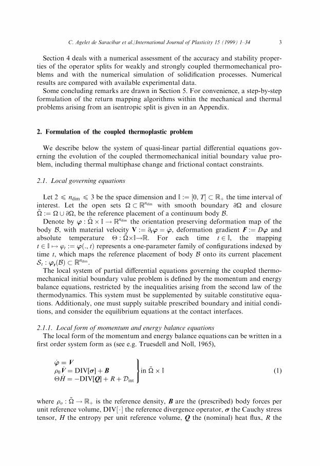
2.1.1. Local form of momentum and energy balance equationsThe local form of the momentum and energy balance equations can be written in a

®rst order system form as (see e.g. Truesdell and Noll, 1965),

_' � V�0 _V � DIV�� B� _H � ÿDIV�Q� � R�Dint

9=;in �� I �1�

where �o : �! R� is the reference density, B are the (prescribed) body forces perunit reference volume, DIV� � � the reference divergence operator, � the Cauchy stresstensor, H the entropy per unit reference volume, Q the (nominal) heat ¯ux, R the

C. Agelet de Saracibar et al./International Journal of Plasticity 15 (1999) 1±34 3

(prescribed) heat source and Dint the internal dissipation per unit reference volume.Formally, the governing equations for a quasi-static case, may be obtained just bysetting �0 � 0 in Eq. (1).

2.1.2. Dissipation inequalitiesThe speci®c entropy H and the Cauchy stress tensor � are de®ned via constitutive

relations, typically formulated in terms of the internal energy E, and subjected tothe following restriction on the internal dissipation, (see e.g. Truesdell and Noll,1965,

Dint � � : _"�� _Hÿ _E50 in �� I �2�

where � :� SYMM�Fÿ I� is the in®nitesimal strain tensor. Here SYMM [.] denotesthe symmetric operator and I is the second order identity tensor.The heat ¯ux Q is de®ned via constitutive equations, say Fourier's law, subjected

to the restriction on the dissipation by conduction

Dcon � ÿ 1

�GRAD��Q50 in �� I �3�

2.1.3. Thermoplastic constitutive equationsMicromechanically based phenomenological models of in®nitesimal strain plasti-

city adopt a local additive decomposition of the strain tensor into elastic and plasticparts. Hardening mechanisms in the material taking place at a microstructural levelare characterized by an additional set of phenomenological internal variables col-lectively denoted here by ��. In the coupled thermornechanical theory. an additivesplit of the local entropy into elastic and plastic parts is adopted, where the plasticentropy is viewed as an additional internal variable arising as a result of dislocationand lattice defect motion. This additive split of the local entropy was adopted byArmero and Simo (1993). The above considerations, motivate the following additivesplit of the in®nitesimal strain tensor � :� �e � �p and local entropy H :� He �HP

and the following set of microstructural internal variables G :� �P;HP; ��

.The internal energy function E depends on the elastic part of the strain tensor �e,

the hardening internal variables �� and the con®gurational entropy He, taking thefunctional form E � E��e;He; ��. Introducing the functional form of the internalenergy into the expression of the internal dissipation, taking the time derivative,applying the chain rule and using the additive split of the in®nitesimal strain tensorand total entropy, a straightforward argument yields the following constitutiveequations and reduced internal dissipation inequality

� :� @�e E��e;He; ��; � :� @HeE��e;He; ��; �� :� ÿ@�� E��e;He; ��;Dint :� Dmech �Dther50;with Dmech :� � : _�p � ��50 and Dther :� � _Hp:

�4�

Using the Legendre transformation � Eÿ�He, the free energy function takesthe functional form � ��e;�; ��. Taking the time derivative of the free energy


function and applying the chain rule, a straightforward argument yields the follow-ing alternative expressions for the constitutive equations

� :� @�e��e;�; ��; He :� ÿ@��e;�; ��; �� :� ÿ@��e;�; �� 5�

Assuming a yield function of the form � � ��; ��;��, the evolution laws of theinternal variables, assuming associated ¯ow, take the form

_�p :� @��; ��;��; _�� :� @��; ��;��; _Hp :� @��; ��;��; �6�

and the following Kuhn±Tucker 50;�40; � � 0 and consistency _� � 0 con-ditions must be satis®ed for a rate-independent plastic model.Additionally, the heat ¯ux is related to the absolute temperature through the

Fourier's law, that for the isotropic case takes the form Q � ÿK GRAD ��.

Remark 1. Equivalent forms of the energy balance equation. Using the additive split ofthe total entropy into elastic and plastic parts and the additive split of the internaldissipation into mechanical and thermal, the reduced energy equation can be expressedas

� _H � ÿDIV�Q� � R�Dmech: �7�

Alternatively, using the constitutive equation of the elastic entropy, taking its timederivative and applying the chain rule, the temperature-form of the reduced energyequation can be written as

c0 _� � ÿDIV�Q� � R�Dmech ÿHep with

c0 :� ÿ�@2��e;�; ��;Hep :� ÿ�@2��e��e;�; �� : _�e ÿ�@2��e;�; �� : _��;

�8�

where c0 is the reference heat capacity andHep the structural elastoplastic heating.

Remark 2. Thermal phase-change contributions. The free energy function for a coupledthermomechanical model including phase change can be splitted into thermoelasticte, thermoplastic tp, thermal (except phase change) t and thermal phase changetpc contributions, taking the functional form, � te��e;�� tp��; ��t�� tpc��.Collecting into a thermoelastoplastic part tep��e;�; �� all the terms appearing into

the free energy function, except the thermal phase change contribution, and settingHe :� He

tep �Hetpc with He

tep :� ÿ@�tep��e;�; �� and Hetpc :� ÿ@�tpc��; the

reduced energy balance equation in entropy form, can be written as

� _Hetep � ÿDIV�Q� � R�Dmech ÿHpc with

Hpc :� _L � � _Hetpc � ÿ�@2��tpc�� _�;

�9�


where Hpc :� _L is the phase-change heating given by the rate of latent heat L per unitreference volume.Similarly, the reference heat capacity can be splitted into c0 � c0tep � c0tpc where

c0tep � ÿ�@2�� tep��e;�; �� and c0tpc � ÿ�@2�� tpc��, and the temperature form ofthe energy balance equation takes the form

c0tep_� � ÿDIV�Q� � R�Dmech ÿHpc ÿHep with

Hpc :� _L � c0tpc_� � ÿ�@2��tpc��:

�10�

Remark 3. Mechanical modeling of the liquid phase. The mechanical behavior in theliquid, for an isothermal liquid±solid phase change at the solidi®cation (melting) tem-perature �m, or in the liquid and mushy zone for a non isothermal liquid-solid phasechange given by the liquidus and solidus temperatures �l and �s, respectively, has beenmodeled by using a modi®ed shear modulus in the liquid phase de®ned asGl � �1ÿ fl�G, where fl 2 �0; 1� is the liquid fraction.For an isothermal phase change, the liquid fraction takes the form

fl�� H��ÿ�m�, where H�� is the Heaviside function. In this case, the gradient ofthe liquid fraction must be interpreted in a distributional sense and takes the formrfl�� ÿ�m�, where �� is the Dirac delta function.For a non-isothermal phase change, a simple de®nition of the liquid fraction is a

piecewise-linear C0 function. Alternatively, a C1 regularized liquid fraction functionmay be introduced, leading to a more convenient modeling from the point of view of therate of convergence of the numerical solution.

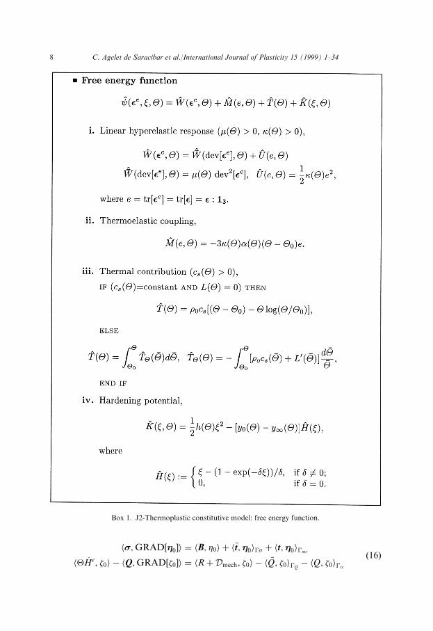
2.2. A J2-thermoplastic constitutive model

Here the following J2-thermoplastic constitutive model described in Boxes 1 and 2has been considered. The thermoplastic and hardening contributions to the freeenergy function presented in Box 1 are uncoupled, as suggested by experimentalresults in Zbedel and Lehmann (1987). All the thermomechanical material propertiesmay be temperature dependent. A particular interest has been placed in consideringthe case in which the speci®c heat is temperature dependent and the latent heat isnon-zero. Note that in this case the functional related to the pure thermal con-tribution is obtained using an integral expression.

2.3. Thermomechanical contact model

Here only a brief summary of the constitutive thermomechanical contact for-mulation will be presented. The interested reader is addressed to Agelet de Saracibar(1997, 1998), and references there in, for further details.Mechanical contact has been modeled by using a penalty regularization technique.

Contact pressure tN has been characterized by a constitutive equation of the form,

tN � d

dgNU��gN�; i:e: U��gN� � 1

2"NhgNi2; �11�


where gN is the normal gap and "N is a normal penalty parameter.The frictional constitutive response is governed by the following constrained pro-

blem of evolution

LvTt[T � "Tv[T ÿ "T@t[T��t[T; tN; ��;_� � k t[T k;

)�12�

where t[T is the frictional traction, v[T is the relative slip velocity, � is the slip hard-ening/softening internal variable, here chosen to be the (accumulated) frictionaldissipation, "T is a tangential penalty parameter, LvT�� denotes the Lie derivativealong the ¯ow generated by the relative slip velocity and and ��t[T; tN; �� are theslip consistency parameter and slip function, respectively, subjected to the followingKuhn-Tucker complementarity and consistency conditions

50; ��t[T; tN; ��40; ��t[T; tN; �� 0;

ddt

��t[T; tN; �� 0 if ��t[T; tN; �� 0:�13�

We refer to Laursen (1992), Laursen and Simo (1991, 1992, 1993a,b) and Agelet deSaracibar (1997, 1998) for further details on the formulation of frictional con-tact problems.A thermal contact model at the contact interface is considered, taking into

account heat conduction ¯ux through the contact surface, heat generation due tofrictional dissipation and heat convection between the interacting bodies when theyseparate one from each other.Heat conduction through the contact surface Qhcond has been assumed to be a

function of the normal contact pressure tN, the mean gas temperature �G and thethermal gap g�, of the form

Qhcond � hcond�tN;�G�g�: �14�

Heat convection between the two bodies arise when they separate from each otherdue to a shrinkage process taking place during solidi®cation. Heat convection coef-®cient has been assumed to be a function of the mechanical gap. Then the heatconvection has been assumed to be modeled as

Qhconv � hconv�gN�g�: �15�We refer to Wriggers and Miehe (1992, 1994) and Agelet de Saracibar, (1997b) forfurther details on the formulation of thermal contact models and thermomechanicalcontact formulations.

2.4. Variational formulation

Using standard procedures, the weak form of the momentum balance (we willassume the quasi-static case for simplicity) and reduced energy equations take thefollowing expressions:


h�;GRAD��0�i � hB; �0i � h �t;�0iÿ� � ht;�0iÿmc

h� _He; �0i ÿ hQ;GRAD��0�i � hR�Dmech; �0i ÿ h �Q; �0iÿQÿ hQ; �0iÿtc

�16�

Box 1. J2-Thermoplastic constitutive model: free energy function.


Box 2. J2-Thermoplastic constitutive model: thermoelastic and thermoplastic responses.


which must hold for any admissible displacement and temperature functions �0 and�0, respectively. We refer to Agelet de Saracibar (1998) for notation and furtherdetails on the derivation of these weak forms and, particularly, on the expressionsrelated to the thermomechanical frictional contact contributions.

3. Time integration of the coupled thermoplastic problem

The numerical solution of the coupled thermornechanical IBVP involves thetransformation of an in®nite dimensional dynamical system, governed by a systemof quasi-linear partial di�erential equations into a sequence of discrete nonlinearalgebraic problems by means of a Galerkin ®nite element projection and a timemarching scheme for the advancement of the primary nodal variables, i.e. displace-ments and temperatures, together with a return mapping algorithm for theadvancement of the internal variables.Here, attention will be placed to the time integration schemes of the governing

equations of the coupled thermoplastic problem. In particular, we are interested in aclass of unconditionally stable staggered solution schemes, based on a product for-mula algorithm arising from an operator split of the governing evolution equations.These methods fall within the classical fractional step methods.

3.1. Local evolution problem

Consider the following (homogeneous) ®rst order constrained dissipative localproblem of evolution, see Simo (1994),

ddt

Z � A�Z;ÿ� in �� 0;T�;Zjt�0 � Z0 in �

)�17�

along with

ddt

ÿ � G�Z;ÿ� in �� 0;T�;ÿjt�0 � 0 in �;

)�18�

where Z, lying in a suitable Sobolev space Z, is a set of primary independent vari-ables, is a set of internal variables, A�Z;ÿ� and G�Z;ÿ� are nonlinear operators and 50 is a multiplier subjected to the classical Kuhn±Tucker conditions for a rate-independent plasticity model. In the formulation of the fractional step methoddescribed below, it is essential to regard the set of internal variables ÿ as implicitlyde®ned in terms of the variables Z via the evolution Eq. (18). Therefore Z are theonly independent variables and their choice becomes a crucial aspect in the for-mulation of the fractional step method. We refer to Simo (1994) for further details.Consider the set of conservation/entropy/latent heat variables Z and the set of

internal variables ÿ de®ned, respectively, as


Z :� ';P;He;HP;L�

and ÿ :� �P; �� 19�

where ' is the deformation map, p :� �0V denotes the material linear momentum,He and HP are the elastic entropy (including phase change contributions) and plasticentropy per unit reference volume, respectively, L is the latent heat per unit refer-ence volume, �p the plastic strain and �� the strain-like hardening variables. Thechoice of Z becomes motivated by the design constraints introduced in the isentropicoperator split described below and it can be considered as an extension to phase-change problems of the choice given in Simo (1994).All the remaining variables in the problem can be de®ned in terms of Z and ÿ by

kinematic and constitutive equations. In particular,

i. The elastic strain �e :� �ÿ �pii. The Cauchy stress tensor � :� @�e E��e;He; �� and stress-like hardening vari-

ables �� :� ÿ@�� E��e;He��:iii. The temperature � :� @HeE��e;He; �� and nominal heat ¯ux

Q � ÿK GRAD��.With these de®nitions in hand, and assuming zero body forces and zero heat

sources, the governing evolution equations of the thermoplastic problem can bewritten in the form given by Eqs. (17) and (18) where the nonlinear operatorsA�Z;ÿ� and G�Z;ÿ� take the form

A�Z;ÿ� :�

1�0 p

DIV��ÿ 1

� DIV�Q� � 1�Dmech

1�Dther

Hpc

8>>>>><>>>>>:

9>>>>>=>>>>>;;G�Z;ÿ� :� @��; ��;��

@��; ��;��

; �20�

where the phase-change heating HPc is given by

Hpc :� ÿ�@2�� tpc��:�; �21�

and the mechanical dissipation Dmech and thermal dissipation Dther are given by

Dmech :� � : G�Z;ÿ�50; Dther :� �@��; ��;��; �22�where, using a compact notation, we denoted as �T :� ��T; �� the generalized stresses.

3.2. A-priori stability estimate

For nonlinear dissipative problems of evolution nonlinear stability can be phrasedin terms of an a-priori estimate on the dynamics of the form

d

dtL�Z;ÿ�40 for t 2 �0;T� �23�

where L�� is a non-negative Lyapunov-like function.


For nonlinear thermoplasticity, see Armero and Simo (1993), consider an exten-ded canonical free energy functional L�� de®ned as

L�Z;ÿ� ��

�jpj2

2�0� E��e;He; �� ÿ�0H

e�d� Vext�'�; �24�

and assume that the following conditions hold:

1. zero heat sources, i.e. R � 0,2. conservative mechanical loading with potential Vext�'�, i.e. B=ÿ@'Vext�'�;3. dirichlet boundary conditions for the temperature ®eld with prescribed con-

stant temperature �0 > 0; i:e:� � �0 on @� I and ÿQ�é.

Then, L�� is a non-increasing Lyapunov-like function along the ¯ow generated bythe thermoplastic problem and a straightforward computation shows that the fol-lowing a-priori stability estimate holds:

d

dtL�Z;ÿ � ÿ

�

�0

��Dmech �Dcon�d40 in �0;T�: �25�

This condition is regarded (see Armero and Simo, 1993), as a fundamental a-prioristability estimate for the thermoplastic problem of evolution which must be preservedby the time-stepping algorithm.

3.3. Operator splits

Consider the dissipative problem of evolution given by Eqs. (17) and (18) with theassociated non-increasing Lyapunov-like function L�� given by Eq. (24). Consideran additive operator split of the vector ®eld A � A�1� � A�2� leading to the followingtwo sub-problems

Problem 1 Problem 2_Z � A�1��Z;ÿ�;

_ÿ � G�Z;ÿ�;�

_Z � A�2��Z;ÿ�;_ÿ � G�Z;ÿ �:

� �26�

The critical restriction on the design of the operator split is that each one of the sub-problems must preserve the underlying dissipative structure of the original problem, i.e.

d

dtL�Z��;ÿ��40; � � 1; 2: �27�

where t 7! �Z��;ÿ�� denotes the ¯ow generated by the vector ®eld A��; � � 1; 2.Two di�erent operator splits will be considered here. First, following Armero and

Simo (1992a,b, 1993) an isentropic operator split, which satis®es the critical designrestriction mentioned above, is considered. This split is compared next with anisothermal operator split, which does not satisfy the design restriction.


3.3.1. The isentropic operator splitConsider the following additive isentropic-based operator split of the vector ®eld

A�Z;ÿ� :

A�Z;ÿ� :� A�1�ise �Z;ÿ� � A

�2�ise �Z;ÿ� �28�

where we de®ne the vector ®elds A�1�ise and A

�2�ise as

A�1�ise �Z;ÿ� :�

1�0 p

DIV��000

8>>>><>>>>:

9>>>>=>>>>;;A�2�ise �Z;ÿ� :�

00

ÿ 1� DIV�Q� � 1

�Dmech

1�Dther

Hpc

8>>>>><>>>>>:

9>>>>>=>>>>>;; �29�

and consider the following two problems of evolution:

Problem 1 Problem 2_Z � A

�1�ise �Z;ÿ�;

_ÿ � G�Z;ÿ�;�

_Z � A�2�ise �Z;ÿ�;

_ÿ � G�Z;ÿ�:�

�30�

Within this operator split, Problem 1 de®nes a mechanical phase at ®xed entropyand Problem 2 de®nes a thermal phase at ®xed con®guration. Note that a strongcondition has been placed in the Problem 1, by the additional requirement that notonly the entropy must remain ®xed, but also the elastic and plastic entropy, as wellas the latent heat. Note also that the evolution of the plastic internal variables isimposed in both problems.Denoting by t 7! �Z��;ÿ�� the ¯ow generated by the vector ®eld A

��ise ; � � 1; 2; a

straightforward computation shows that the following stability estimates hold:

d

dtL�Z�1�;ÿ�1�� ÿ

�

D�1�mechd40d

dtL�Z�2�;ÿ�2�� ÿ

�

�0

��2��D�2�mech �D�2�con�d40;

�31�

where D��mech;D��con and �� are the mechanical dissipation, thermal heat conductiondissipation and absolute temperature, respectively, in Problem �; � � 1; 2.Thus, the isentropic split preserves the underlying dissipative structure of the ori-

ginal problem.

3.3.2. The isothermal operator splitConsider the following additive isothermal-based operator split of the vector ®eld

A�Z;ÿ�:A�Z;ÿ� :� A

�1�iso�Z;ÿ� � A

�2�iso�Z;ÿ�; �32�

where we de®ne the vector ®elds A�1�iso and A

�2�iso as


A�1�iso�Z;ÿ� :�

1�0 p

DIV��1�H

ep

00

8>>>>><>>>>>:

9>>>>>=>>>>>;;A�2�iso�Z;ÿ� :�

00

ÿ 1� DIV�Q� � 1

� �Dmech ÿHep�1�Dther

Hpc

8>>>>><>>>>>:

9>>>>>=>>>>>;;

�33�

and consider the following two problems of evolution:

Problem 1

_Z � A�1�iso�Z;ÿ�;

_ÿ � G�Z;ÿ�;� Problem 2

_Z � A�2�iso�Z;ÿ�;

_ÿ � G�Z;ÿ�:� �34�

Within this operator split, Problem 1 de®nes a mechanical phase at ®xed tem-perature and Problem 2 de®nes a thermal phase at ®xed con®guration. Note also,that the evolution of the plastic internal variables ÿ is imposed in both problems.

Denoting by t 7!�Z��ÿ�� the ¯ow generated by the vector ®eld A��iso ; � � 1; 2; a

straightforward computation shows that the following stability estimates hold:

d

dtL�Z�1�;ÿ�1�� ÿ

�

D�1�mechd��

�1ÿ �0

��1��Hep�1�d40;

d

dtL�Z�2�;ÿ�2�� ÿ

�

�0

��2��D�2�mech �D�2�con�dÿ

�

�1ÿ �0

��2��Hep�2�d40;

�35�where D��mech;D��con;Hep�� and �� are the mechanical dissipation, thermal heatconduction dissipation, structural elastoplastic heating and absolute temperature,respectively, in Problem �; � � 1; 2.The contribution of the structural elastoplastic heating to the evolution equations

of each one of the problems arising from the isothermal operator split, breaks theunderlying dissipative structure of the original problem.

3.4. Product formula algorithms

The additive operator split of the governing evolution equations leads to a pro-duct formula algorithm and to a staggered solution scheme of the coupled problem,in which each one of the subproblems is solved sequentially. Remember that the setof internal variables ÿ is viewed as implicitly de®ned in terms of the set of variablesZ, which are considered to be the only independent variables. Therefore, our interesthere is placed on the time discrete version of the evolution Eq. (17), and the updatein time of the variables Z using a time-stepping algorithm.Consider algorithms K

��t � � � being consistent with the ¯ows t 7!�Z��;ÿ��;

� � 1; 2; and dissipative stables, i.e. which inherit the a-priori stability estimate onthe dynamics given by Eq. (27). Then the algorithm de®ned by the product formula:


K�t� � � � K�2��t �K

�1��t

� �� 36�

is also consistent and dissipative stable. For dissipative dynamical systems if each ofthe algorithms is unconditionally dissipative stable, then the product formula algo-rithm is also unconditionally dissipative stable. This product formula algorithm isonly ®rst order accurate. A second order accurate product formula algorithm can bede®ned through a double pass technique given by (see Strang, 1969),

K�t� � � � K�1��t=2 �K

�2��t �K

�1��t=2

� �� : �37�

Note that, according to Eqs. (31) and (35), algorithms based on the isothermaloperator split will result in staggered schemes at best only conditionally stables andonly an isentropic operator split leads to unconditionally (dissipative) stable productformula algorithms.

3.5. Time discrete variational formulation

The use of an operator split, applied to the coupled system of nonlinear ordinarydi�erential equations, and a product formula algorithm, leads to a staggered algorithmin which each one of the subproblems de®ned by the partition is solved sequentially,within the framework of classical fractional step methods. We note that contrary tocommon practice, the evolution equations for the microstructural internal variablesare enforced in both phases of the operator split, as in Armero and Simo (1992b,1993, 1994). A Backward±Euler (BE) time stepping algorithm has been used andtwo di�erent operator±splits have been considered.

3.5.1. Isentropic splitIn the isentropic split, ®rst introduced by Armero and Simo (1992a,b, 1993) the

coupled problem is partitioned into a mechanical phase at constant entropy, fol-lowed by a thermal phase at ®xed con®guration, leading to an unconditionally stablestaggered scheme. The additional design constraints of constant elastic and plasticentropy and latent heat, in the isentropic mechanical phase have been introduced.An e�cient implementation of the split can be done using the temperature as pri-mary variable. See Armero and Simo (1992a,b, 1993) and Simo (1994) for furtherdetails.

3.5.1.1. Mechanical phase. The mechanical problem is solved at constant entropy.For the sake of simplicity, only the quasi-static case will be considered. According tothe de®nition ofZ given by Eq. (19) and the operator split given by Eqs. (28)±(30), theadditional design constraints of constant elastic and plastic entropy and latent heat,have been introduced. The evolution of the temperature can be computed locally.The time discrete weak form of the momentum balance and the local updates ofelastic and plastic entropy, latent heat and internal variables, take the form:


h ~�n�1;GRAD��0�i � hB;�0i � h �tn�1;�0iÿ� � htn�1;�0iÿmc

~Hen�1 � He

n;

~Hpn�1 � Hp

n;

~Ln�1 � Ln;

ÿn�1 � ÿn � ~ n�1 ~Gn�1;

9>>>>>>>=>>>>>>>;�38�

and the temperature is locally updated according to ~�n�1 � @HeE� ~�en�1;Hen;

~��n�1�.

3.5.1.2. Thermal phase. Using a BE scheme the time discrete weak form of the energybalance equation and updated elastic and plastic entropy, latent heat and internalvariables in the thermal phase take the form:

1

�th�n�1�He

n�1 ÿHen�; �0i ÿ hQn�1;GRAD��0�i �

hR�Dmechn�1 ; �0i ÿ h �Qn�1; �0iÿQÿ hQn�1; �0iÿtc

Hen�1 � ÿ@��en�1;�n�1; ��n�1�;

Hpn�1 � Hp

n ��t

�n�1Dthern�1 ;

Ln�1 � L��n�1�;ÿn�1 � ÿn � n�1Gn�1:

9>>>>>>>>>>>>>=>>>>>>>>>>>>>;�39�

3.5.2. Isothermal splitIn the isothermal split the coupled system of equations is partitioned into a mechan-

ical phase at constant temperature, followed by a thermal phase at ®xed con®guration.Note that, within the context of the product formula algorithm, using the entropy formof the energy equation, the elastic entropy computed at the end of the mechanical par-tition is used as initial condition for the solution of the thermal partition.

3.5.2.1. Mechanical phase. Noting that under isothermal conditions the plasticentropy and latent heat remain constant, the time discrete weak form of themomentum balance equation, updated elastic and plastic entropy, latent heat andinternal variables take the form:

h ~�n�1;GRAD��0�i � hB;�0i � h �tn�1;�0iÿ� � htn�1;�0iÿmc

~Hen�1 � ÿ@�� ~�en�1;�n; ��n�1�;

~Hpn�1 � Hp

n;

~Ln�1 � Ln;

~ÿn�1 � ÿn � ~ n�1 ~Gn�1;

9>>>>>>>=>>>>>>>;�40�

3.5.2.2. Thermal phase. Using a BE scheme the time discrete weak form of the energybalance equation and updated elastic and plastic entropy, latent heat and internalvariables take the form:


1

�th�n�1�He

n�1ÿ ~Hen�1�; �0i ÿ hQn�1;GRAD��0�i �hR�Dmechn�1 ÿHep

n�1; �0i ÿ h �Qn�1; �0iÿQ ÿ hQn�1; �0iÿtc

Hen�1 � ÿ@��en�1;�n�1; ��n�1�;

Hpn�1 � Hp

n ��t

�n�1Dthern�1 ;

Ln�1 � L��n�1�;ÿn�1 � ÿn � n�1Gn�1:

9>>>>>>>>>>>>>=>>>>>>>>>>>>>;�41�

4. Numerical simulations

The formulation presented in the previous sections is illustrated here in a numberof representative numerical simulations. First a numerical assessment of the accu-racy and stability behavior of the isothermal and isentropic operator splits is pre-sented in the context of quasi-static and fully dynamic cooling analysis of athermoelastic and thermoplastic pressurized thick walled cylinder. Next, the goalsare to provide a practical accuracy assessment of the themiomechanical model and todemonstrate the robustness of the overall coupled thermomechanical formulation in anumber of solidi®cation examples, including industrial processes. The computationsare performed with the ®nite element code COMET developed by the authors. TheNewton±Raphson method, combined with a line search optimization procedure, isused to solve the nonlinear system of equations arising from the spatial and temporaldiscretization of the weak form of the momentum and reduced dissipation balanceequations. Convergence of the incremental iterative solution procedure was mon-itored by requiring a tolerance of 0.1% in the residual based error norm.

Fig. 1. Cooling of a pressurized thick-walled cylinder. Initial geometry and boundary conditions.


4.1. Numerical assessment of the operator split algorithms

4.1.1. Cooling of a thermoelastic/thermoplastic thick walled cylinderIn this problem a quasi-static and fully dynamic cooling analysis of a thermo-

elastic and thermoplastic pressurized thick walled cylinder is presented. The goals

Fig. 2. Quasi-static cooling of a thermoelastic pressurized thick-walled cylinder. Radial displacement and

temperature at the inner and outer surfaces. Using isentropic and isothermal operator splits, for a weakly

coupled (Case 1) and strongly coupled (Case 2) cases.


here are to provide a numerical assessment of the accuracy and stability behaviorshowed by the isothermal and isentropic operator splits, in weakly (Case 1) andstrongly (Case 2) coupled problems. To get a strongly coupled problem, the thermalexpansion coe�cient a has been, unrealistically, multiplied by a factor of 6 in thequasi-static cases and by a factor of 3 in the fully dynamic cases.

Fig. 3. Quasi-static cooling of a thermoplastic pressurized thick-walled cylinder. Radial displacement and




Figure 1 depicts the initial geometry of the problem, as well as the prescribedboundary conditions. Plane strain conditions are assumed in the axial direction, sothat a unit band of axisymmteric ®nite elements need only be considered. The innerand outer radii adopted are Ri=100mm and RO=200mm, respectively. The mate-rial properties are assumed to be (linearly) temperature dependent. The initial tem-

Fig. 4. Dynamic cooling of a thermoelastic pressurized thick-walled cylinder. Radial displacement and




perature of the cylinder is 593K, while the reference (ambient) temperature is 293K.Di�erent (constant) convection coe�cients are considered for the inner, h=1.16N/mm sK. and outer, h=0.01N/mm sK, surfaces. The simulations are performed byapplying a pressure of 200N/mm2 at the inner face of the cylinder. Standard bi-lin-ear isoparametric axisymmetric ®nite elements are employed.

Fig. 5. Dynamic cooling of a thermoplastic pressurized thick-walled cylinder. Radial displacement and




The results obtained for the quasi-static analyses are collected in Figs. 2 and 3 fora thermoelastic and a thermoplastic constitutive response, respectively. Figures 4 and5 collect the results obtained for the fully dynamic analysis, assuming a ther-moelasticand a thermoplastic constitutive response, respectively. In each of these ®gures, it isshown for the Cases 1 and 2, the radial displacement and temperature evolutions atthe inner and outer surfaces, obtained using isentropic and isothermal operator

Fig. 6. Solidi®cation of an aluminium cylinder in a steel mould. Geometry of the problem.

Fig. 7. Solidi®cation of an aluminium cylinder in a steel mould. (a) Temperature evolution at the casting

center, casting surface and mould surface for an intermediate section. (b) Radial displacement evolution

at the casting surface and mould surface for an intermediate section.


splits. As expected, these ®gures show that for strongly coupled problems (Case 2)the isothermal split leads to a completely unstable behavior ending with a blow-upof the solution. while the isentropic split provides the right solution. Despite thisfact, for weakly coupled problems the two splits provide practically the same solu-tion. This behavior has been shown in quasi-static and dynamic analyses, as well mfor thermoplastic and thermoplastic constitutive responses.

4.2. Numerical simulations of solidi®cation processes

4.2.1. Cylindrical aluminium solidi®cation testThis example, taken from Celentano et al. (1996), is concerned with the solidi®-

cation process of a cylindrical aluminium specimen in a steel mould. The geometryof the problem is shown in Fig. 6. Assumed starting conditions in the numericalsimulation are given by a completely ®lled mould with aluminium in liquid state at auniform temperature of 670�C. The initial temperature of the mould is 200�C. Thematerial properties for the aluminium have been assumed to be temperature depen-dent, while constant material properties have been assumed for the steel mould. Theexternal surfaces of themould aswell as the upper surface of the castingmetal have beenassumed perfectly insulated. A constant heat transfer coe�cient hco � 10 N=mm s Kand a gap dependent convection±radiation coe�cient between the aluminium and thesteel mould has been assumed. Only gravitational forces have been assumed. Furtherdetails on the geometrical and material data can be found in the above reference.Spatial discretization of the casting cylinder and the mould has been done using a

®nite element mesh of axisymmetric 3-noded triangles. Numerical simulation wasdone up to 90 s. of the solidi®cation test using a time increment of 1 s.Figure 7(a) shows the temperature evolution at the casting center, casting surface

and mould surface for an intermediate section. A typical temperature plateau due tothe release of latent heat during solidi®cation can be seen in the casting center point ofthis section up to 15 s approximately. Figure 7(b) shows the evolution of the radialdisplacements at the casting and mould surfaces for the same intermediate section.The di�erence between the two curves gives the gap distance evolution at the chosensection. Temperature and air gap evolution predicted by the model compare very well

Fig. 8. Solidi®cation of a Renault Clio crankshaft. Finite element mesh of the part.


Fig. 9. Solidi®cation of a Renault Clio crankshaft. Temperature distribution at di�erent stages of the

solidi®cation process.



solidi®cation process. Section x±y.



solidi®cation process. Section x±z.


Fig. 12. Solidi®cation of a Renault Clio crankshaft. Evolution of the mushy zone. Temperature dis-

tribution at di�erent stages of the solidi®cation process. Sections x±y and x±z.


with experimental results. A data sensitivity analysis has shown a strong in¯uence ofthe heat convection coe�cient, between aluminium and mould, in the temperatureevolution.

4.2.2. Solidi®cation of a Renault Clio crankshaftThis example deals with the numerical simulation of the solidi®cation process of

an industrial part, in this case, a Renault Clio crankshaft. Geometrical and materialdata, as well as experimental results, were provided by Renault. Fig. 8 shows a viewof the ®nite element mesh used for the part, consisting of nearly 15000 4-noded tet-

Fig. 13. (a) Solidi®cation of a Renault Clio crankshaft. Temperature evolution at di�erent points.


rahedral elements. The sand mould has been discretized using around another 300004-noded tetrahedral elements.The temperature distribution at the part at di�erent stages of the analysis, using a

quarter section view, is shown in Figs. 9±11 show the temperature distribution onsections x±y and x±z, respectively, of the deformed shape of the part. In these Fig-ures it is also clearly shown the evolution of the gap between the part and the mould.The evolution of the mushy zone, given by the temperature evolution at the liquid±solid transition phase, is shown in Fig. 12. A comparison between the computed andthe experimental temperature evolution at di�erent points is shown in Fig. 13(a) and(b), where a good agreement is observed.

Fig. 13. (b) Solidi®cation of a Renault Clio crankshaft. Temperature evolution at di�erent points.


5. Concluding remarks

A formulation of coupled thermoplastic problems with phase-change has beenpresented. The formulation has been consistenly derived within a thermodynamicframework. A particular J2 thermoplastic model has been considered in which thematerial properties have been assumed to be temperature dependent. Operator splitsof the governing di�erential equations, and their nonlinear stability properties, havebeen discussed. Within the isentropic operator split, additional split design con-straints have been introduced. A numerical assessment of the accuracy and non-linear stability properties of the isentropic and isothermal splits has been performed.Numerical results obtained in the simulation of solidi®cation processes show a goodagreement with the experimental data available.

Acknowledgements

Financial support for this work has been provided by Renault under contractCIMNE/1997/001-A�ectation: H5.21.41 with CIMNE. This support is gratefullyacknowledged.

Appendix A. Return mapping algorithms

In this appendix we summarize the main steps involved in the return mappingalgorithms for the mechanical and thermal problems arising from the isentropicoperator split. Note that for the mechanical problem an isentropic return mappingalgorithm is performed, while for the thermal problem the classical isothermalreturn mapping is performed.

A.1. Mechanical problem

A.1.1. Step 1: trial state (kinematics)

Given the initial data �n;�nf g and database �pn; �n�

at time tn and prescribed �n�1at time tn�1, set:

�p trialn�1 :� �pn;�trialn�1 :� �n;

�e trialn�1 :� �n�1 ÿ �p trial

n�1 :

A.1.2. Step 2: trial temperature

IF (constant material properties) THEN


�trialn�1 :� ��en�1;He

n; �trialn�1� with en�1 :� tr��n�1� and He

n :� He�en;�n; �n�;

ELSESolve for �trial

n�1 the implicit nonlinear equation:

He�en�1;�trialn�1; �

trialn�1� ÿHe

n � 0:

END IF

A.1.3. Step 3: trial (generalized) stresses

strialn�1 :� dev��trial

n�1� � 2�trialn�1dev��e trial

n�1 �;ptrialn�1 :� ktrial

n�1en�1 ÿ 3�trialn�1�

trialn�1��trial

n�1 ÿ�0�;qtrialn�1 :� ÿK��trial

n�1;�trialn�1�:

A.1.4. Step 4: trial yield function

�trialn�1 :� ��trial

n�1; qtrialn�1;�n� �k strial

n�1 k ÿ��2

3

r�y0��n� ÿ qtrial

n�1�

IF �trialn�140 THEN

Set ��n�1 :� ��trialn�1 and update database

RETURNEND IF

A.1.5. Step 5: isentropic return mapping

IF (constant material properties) THENSolve for n�1 the implicit nonlinear equation:

�n�1 :� ��n�1; qn�1;�n� � 0 with �n�1 � ��en�1;Hen; �n�1�;

ELSESolve for n�1 and �n�1 the implicit nonlinear set of equations:

�n�1 :� ��n�1; qn�1;�n� � 0;He�en�1;�n�1; �n�1� ÿHe

n � 0;

�END IF


�n�1 :�k strialn�1 k

�n�1�trialn�1ÿ 2�n�1 n�1 ÿ

��2

3

r� 0��n� ÿ qn�1�;

�n�1 � �trialn�1 �

��2

3

r n�1;

qn�1 � ÿK��n�1;�n�1�:

A.1.6. Step 6: update database and compute stresses

�pn�1 � �p trialn�1 � n�1ntrial

n�1;

sn�1 � strialn�1

�n�1�trialn�1ÿ 2�n�1 n�1ntrial

n�1;

pn�1 � kn�1en�1 ÿ 3kn�1�n�1��n�1 ÿ�0�;�n�1 � pn�113 � sn�1;

where

ntrialn�1 :� strial

n�1= k strialn�1 k :

A.2. Thermal problem

A.2.1. Step 1: trial state (kinematics)

Given the initial data �n;�nf g and database �pn; �n�

at time tn and prescribed�n�1;�n�1f g at time tn�1, set:

�p trialn�1 :� �pn;�trialn�1 :� �n;�e trialn�1 :� �n�1 ÿ �p trial

n�1 :

A.2.2. Step 2: trial (generalized) stresses

strialn�1 :� dev��trial

n�1� � 2�n�1dev��e trialn�1 �; qtrial

n�1 :� ÿK��trialn�1;�n�1�:

A.2.3. Step 3: trial yield function

�trialn�1 :� ��trial

n�1; qtrialn�1;�n�1� �k strial

n�1 k ÿ��2

3

r�y0��n�1� ÿ qtrial

n�1�


IF �trialn�140 THEN

Set � � �n�1 :� ��trialn�1 and update database

RETURNEND IF

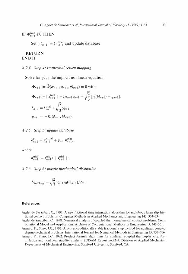
A.2.4. Step 4: isothermal return mapping

Solve for n�1 the implicit nonlinear equation:

�n�1 :� ��n�1; qn�1;�n�1� � 0 with

�n�1 :�k strialn�1 k ÿ2�n�1 n�1 �

��2

3

r�y0��n�1� ÿ qn�1�;

�n�1 � �trialn�1 �

��2

3

r n�1;

qn�1 � ÿK��n�1;�n�1�:

A.2.5. Step 5: update database

�pn�1 � �p trialn�1 � n�1ntrial

n�1;

where

ntrialn�1 :� strial

n�1= k strialn�1 k :

A.2.6. Step 6: plastic mechanical dissipation

Dmechn�1 ��2

3

r n�1y0��n�1�=�t:

References

Agelet de Saracibar, C., 1997. A new frictional time integration algorithm for multibody large slip fric-

tional contact problerns. Computer Methods in Applied Mechanics and Engineering 142, 303±334.

Agelet de Saracibar, C., 1998. Numerical analysis of coupled thermomechanical contact problems. Com-

putational Model and Applications. Archives of Computational Methods in Engineering, 5, 243±301.

Armero, F., Simo, J.C., 1992. A new unconditionally stable fractional step method for nonlinear coupled

thermomechanical problems. International Journal for Numerical Methods in Engineering 35, 737±766.

Armero F., Simo, J.C., 1992. Product formula algorithms for nonlinear coupled thermoplasticity: for-

mulation and nonlinear stability analysis. SUDAM Report no.92±4. Division of Applied Mechanics,

Department of Mechanical Engineering, Stanford University, Stanford, CA.


Armero, F., Simo, J.C., 1993. A priori stability estimates and unconditionally stable product algorithms

for nonlinear coupled thermoplasticity. International Journal of Plasticity 9, 749±782.

Celentano, D., Oller, S., OnÄ ate, E., 1996. A coupled thermornechanical model for the solidi®cation of cast

metals. Int. J. Solids Struct. 33(5), 647±673.

Laursen, T.A., 1992. Formulation and treatment of frictional contact problems using ®nite elements.

Report no.92±6. Ph.D. dissertation, Stanford University, CA.

Laursen, T.A., Govindjee, S., 1994. A note on the treatment of frictionless contact between non-smooth

surfaces in fully non-linear problems. Communications in Applied Numerical Methods 10, 869±878.

Laursen, T.A. Simo, J.C., 1991. On the formulation and numerical treatment of ®nite deformation fraic-

tional contact problems, In: Wriggers, P., Wanger, W. (eds.), Nonlinear Computational Mechanics-

State of the Art. Springer±Verlag, Berlin, pp. 716±736.

Laursen, T.A., Simo, J.C., 1992. Formulation and regularization of frictional contact problems for

lagrangian ®nite element computations. In: Owen, D.R.J., OnÄ ate, E., Hilton, E. (eds.), Proc. of The

Third International Conference on Computational Plasticity: Fundamentals and Applications, COM-

PLAS III. Pineridge Press, Swansea, UK, pp. 395±407.

Laursen, T.A., Simo, J.C., 1993. A continuum-based ®nite element formulation for the implicit solution of

multi-body, large deformation frictional contact problems. International Journal for Numerical Meth-

ods in Engineering 36(20), 3451±3485.

Laursen, T.A., Simo, J.C., 1993. Algorithmic symmetrization of coulomb frictional problems using aug-

mented lagrangians. Computer Methods in Applied Mechanics and Engineering 108, 133±146.

Simo, J.C., 1994. Numerical analysis aspects of plasticity. In: Ciarlet, P.G., Lions, J.J. (eds.), Handbook

of Numerical Analysis, Vol IV. North Holland.

Simo, J.C., Armero, F., 1991. Recent advances in the formulation and numerical analysis of thermo-

plasticity at ®nite strains. In: Stein, E., Besdo, D. (eds.), Finite Inelastic DeformationsÐTheory and

Applications. IUTAM/IACM Symposium, Hannover, FRG, 19±23, August. Springer±Verlag, Berlin,

1991.

Simo, J.C., Miehe, C., 1992. Associative coupled thermoplasticity at ®nite strains: formulation, numerical

analysis and implementation. Computer Methbds in Applied Mechanics and Engineering 98, 41±104.

Strang, G., 1969. Approximating semigroups and the consistency of di�erence schemes. Proc. American

Mathematical Society 20, 1±7.

Truesdell, C., Noll, W., 1965. The nonlinear ®eld theories of mechanics. In: Fluegge, S. (ed.), Handbuch

der Physics Bd. III/3, Springer±Verlag, Berlin.

Wriggers, P., Miehe, C., 1992. Recent advances in the simulation of thermomechanical contact processes.

In: Owen, D.R.J., OnÄ ate, E., Hilton, E. (eds.), Proc. of The Third International Conference on Com-

putational Plasticity: Fundamentals and Applications, COMPLAS III. Pineridge Press, Swansea, UK,

pp. 325±347.

Wriggers, P., Miehe, C., 1994. Contact constraints within coupled thermomechanical analysis. A ®nite

element model. Computer Methods in Applied Mechanics and Engineering 113, 301±319.

Wriggers, P., Zavarise, G., 1993. Thermomechanical contact. A rigorous but simple numerical approach.

Computers and Structures 46, 47±53.

Zdebel, U., Lehmann, T., 1987. Some theoretical considerations and experimental investigations on a

constitutive law in thermoplasticity. International Journal of Plasticity 3, 369±389.


on the formulation of coupled thermoplastic problems with

Documents