on the integro-differential equation associated with ...yantipov/antgaojerry.pdf · on the...

ON THE INTEGRO-DIFFERENTIAL EQUATION ASSOCIATEDWITH DIFFUSIVE CRACK GROWTH THEORY

by Y. A. ANTIPOV†

(Department of Mathematics, Louisiana State University, Baton Rouge, LA 70803, USA)

T.-J. CHUANG‡

(Ceramics Division, National Institute of Standards and Technology, Gaithersburg,MD 20899, USA)

and H. GAO§

(Max Planck Institute for Metals Research, Seestrasse 92, Stuttgart 70174, Germany)

[Received 4 November 2002]

Summary

At high temperatures, polycrystalline materials often suffer creep fracture under prolongedloading conditions. Microstructural examinations reveal that nucleation, propagation andlinkage of interfacial cracks normal to the principal stress directions are responsible for thepremature failure. To simulate service conditions, a semi-infinite crack is considered to grow,in steady state, along a grain boundary via a coupled process of surface and grain-boundarydiffusion within an elastic bi-crystal subjected to a remote constant applied stress. Governingequations based on equilibrium and Hooke’s law obeyed within the adjoining grains, and matterconservation and Fick’s diffusion laws prevailing at both crack surfaces and the interface areemployed to derive the singular integro-differential equation for the normal stress distributionalong the interface ahead of the moving crack tip.

Using the Mellin transformation, the integral equation is first converted to a functional-difference equation (a Carleman boundary-value problem), and then solved analytically viaan approach based on the theory of the Riemann–Hilbert problem on a curve. Asymptoticbehaviours of the stress solutions at both ends (that is, near the crack tip as well as in thefar field) are provided. Excellent agreement is reached when the full analytical solutions arecompared with the existing numerical solutions.

The stress solutions permit the far-field loading intensity to be connected with the boundaryconditions containing the parameter of crack velocity at the crack tip, thereby making it possibleto predict the crack-growth rate for a given applied stress. The stress solutions in analytical formhave the merit, over the numerical form, that they will facilitate the future solution scheme whenthe analysis is extended to tackle crack growth in the transient creep stage wherein both stressesand near-tip crack shapes are changing continuously with time.

1. Introduction

This paper aims to provide analytical solutions for a class of integro-differential equations thatemerge from the diffusional crack-growth theory. Crack-like cavities at grain boundaries are often

† 〈[email protected]〉‡ 〈[email protected]〉§ 〈[email protected]〉

c© Oxford University Press 2003; all rights reserved.Q. Jl Mech. Appl. Math. (2003) 56 (2), 289–310

290 Y. A. ANTIPOV et al.

detected in creep rupture specimens of polycrystalline materials such as metals, metal alloys andceramics. It is believed that their growth and coalescence lead to premature failure. In particular,the growth rate of such cavities may become the dominant contributor to creep life, and developmentof predictive capability of the crack-growth rate as a function of applied stress, which makeslife prediction possible, will be a challenging task for the design engineers and manufacturers ofstructural components in high temperature, load-bearing environments.

A literature review shows that the kinetics of cavity growth may involve coupled mass transportat crack surfaces and grain boundary (that is, surface and grain-boundary self-diffusion); see, forexample, the books by Riedel (1) and Ashby and Brown (2). In (3) Chuanget al. reviewed thesubject of diffusive cavitation along grain interfaces and laid down the conditions under which thegrowth of crack-like cavities prevails. In general, crack-like or slit shapes are favoured if the appliedstress and grain-boundary diffusivity are larger than the sintering stress and surface diffusivity,respectively. Likewise, if the service time approaches the later stage in the growth phase, creepcavities tend to turn into crack-like shapes. Under these circumstances, the crack travels at asubcritical speed in a steady-state fashion along the grain boundary (gb). It is then appropriate totreat the crack as semi-infinite, propagating at a constant speed in an infinite elastic bicrystal underplane-strain conditions. This case has been considered by Chuang (4) and Chuanget al. (5) whosolved the coupled problem of diffusion and elastic deformation, leading to a specific kinetic lawfor subcritical crack growth. The essential part of their work involved solving a singular integralequation. Unfortunately, only numerical solutions were provided in their work. It is inconvenientto expand the coverage to the non-steady-state regime based on their work in numerical form. Toextend the analysis, closed form solutions are desirable. Accordingly, the main objective of thepresent paper is to present complete analytical solutions in closed form, thereby facilitating futurework on more general time-dependent problems.

The program of the current paper is as follows: first, we will briefly describe the diffusionalcrack growth theory, and then using the governing mechanics and physical laws derive the integralequation in section 2. Next, in section 3, in order to solve the integral equation, we convert it intoa functional-difference equation, via the Mellin transformation technique and the Cauchy theorem.We then proceed to tackle the mathematical problem by the method based on the theory of theRiemann–Hilbert problem on an arc (see Antipov and Gao (6)). In section 4, we present theasymptotic solution near the crack tip. The far-field solutions are presented in section 5. A completeclosed-form solution is given in section 6. Finally in section 7, numerical evaluations are made forthe integral representation using the numerical quadrature. The full distribution of stress aheadof the crack tip is determined. The complete solutions are shown to agree with the asymptoticsolutions both near the crack tip and at the far field. Moreover, excellent agreement is reached whenour analytical solutions are compared with the numerical solutions given by Chuang (4), includingstress solutions and stress intensity versus crack-velocity relations. Concluding remarks are given atthe end in section 8. The Appendix extends the solution scheme to a more general class of integralequations which may or may not have any physical implications.

2. Formulation of the physical problem

2.1 Description of the crack-growth model by diffusion

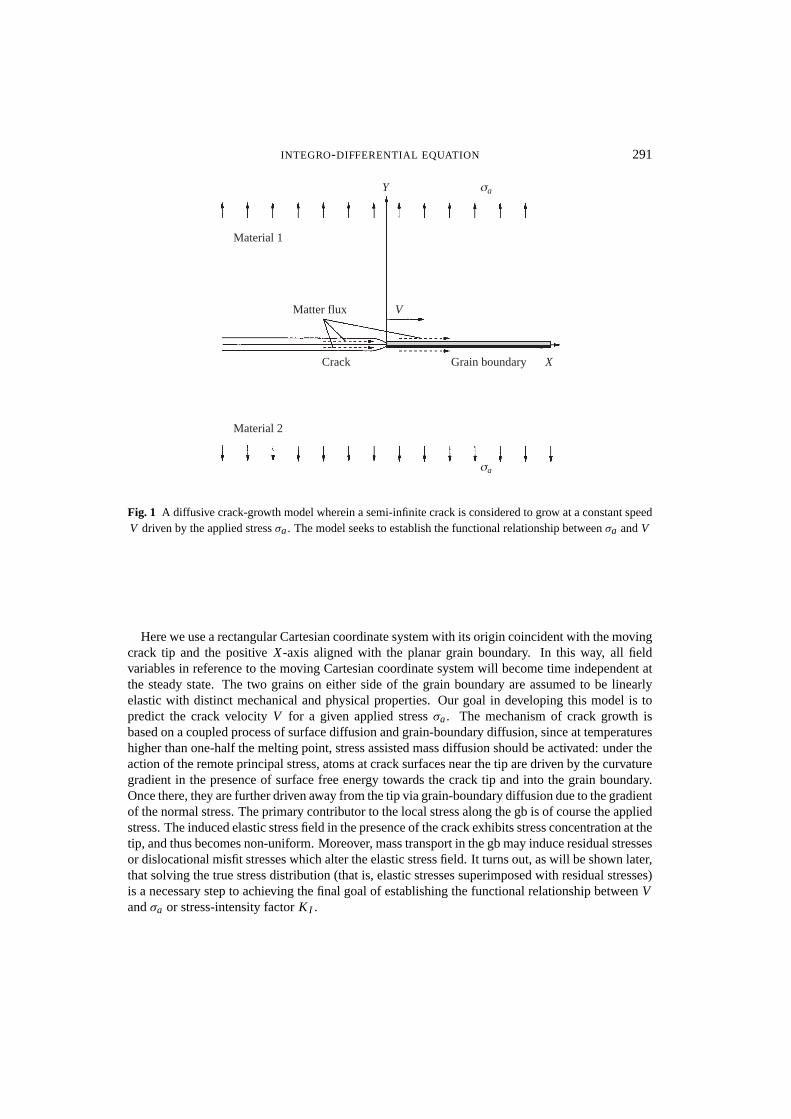
Let us consider a semi-infinite crack travelling in steady state at a constant, unknown a priori,velocity V along a grain boundary between two dissimilar grains under the action of a remoteapplied stressσa (Fig. 1).

INTEGRO-DIFFERENTIAL EQUATION 291

Material 1

Matter flux

Crack

V

Material 2

Grain boundary

Y a

a

X

Fig. 1 A diffusive crack-growth model wherein a semi-infinite crack is considered to grow at a constant speedV driven by the applied stressσa . The model seeks to establish the functional relationship betweenσa andV

Here we use a rectangular Cartesian coordinate system with its origin coincident with the movingcrack tip and the positiveX -axis aligned with the planar grain boundary. In this way, all fieldvariables in reference to the moving Cartesian coordinate system will become time independent atthe steady state. The two grains on either side of the grain boundary are assumed to be linearlyelastic with distinct mechanical and physical properties. Our goal in developing this model is topredict the crack velocityV for a given applied stressσa . The mechanism of crack growth isbased on a coupled process of surface diffusion and grain-boundary diffusion, since at temperatureshigher than one-half the melting point, stress assisted mass diffusion should be activated: under theaction of the remote principal stress, atoms at crack surfaces near the tip are driven by the curvaturegradient in the presence of surface free energy towards the crack tip and into the grain boundary.Once there, they are further driven away from the tip via grain-boundary diffusion due to the gradientof the normal stress. The primary contributor to the local stress along the gb is of course the appliedstress. The induced elastic stress field in the presence of the crack exhibits stress concentration at thetip, and thus becomes non-uniform. Moreover, mass transport in the gb may induce residual stressesor dislocational misfit stresses which alter the elastic stress field. It turns out, as will be shown later,that solving the true stress distribution (that is, elastic stresses superimposed with residual stresses)is a necessary step to achieving the final goal of establishing the functional relationship betweenVandσa or stress-intensity factorK I .


2.2 Governing equations

2.2.1 Derivation of the singular integro-differential equation for stress. As discussed in section2.1, the real stress consists of two terms: the elastic stress and the dislocational misfit stress due todiffusion. To formulate the latter term, consider an edge dislocation residing at an arbitrary locationX = X0 in the gb ahead of the crack tip. The elastic stress field generated by this dislocation andby the applied stress has the following expression (7):

σyy + iσxy = σa − π iλβ(by + ibx )δ(X − X0) − λ(by + ibx )

X − X0, (2.1)

wherei = √−1, bx andby are the Burger’s vectors in theX andY directions, respectively,δ(X) isthe Dirac delta function andλ andβ are Dundurs’s constants. To simulate the residual stress, let usconsider an arbitrary distribution of dislocations along theX -axis under the action of a remote stressσa such thatdby = �′

yd X , dbx = �′x d X . The normal stress at any locationX can be integrated to

yield the following form:

σyy(X) = σa − λ

∫ ∞

−∞�′

y(X0)d X0

X − X0+ πλβ�′

x (X). (2.2)

The shear stress becomes

σxy(X) = −λ

∫ ∞

−∞�′

x (X0)d X0

X − X0− πλβ�′

y(X). (2.3)

Assume that the flat gb cannot resist shear, that is,σxy = 0 everywhere along the wholeX -axis,which is true in many realistic situations. Applying the Hilbert transformation, we have

�′x (X) = β

π

∫ ∞

−∞�′

y(X0)d X0

X − X0. (2.4)

Substituting equation (2.4) in (2.2) and applying the Hilbert transformation again we arrive at

π2λ(1 − β2)�′y(X) =

∫ ∞

0

σyy(X0)d X0

X − X0. (2.5)

Notice that the integration now starts at zero, rather than from minus infinity because of the traction-free conditions at the crack plane in the negativeX -axis. An additional relation between�y andσyy

coming from the grain-boundary diffusion equation (Fick’s law) and steady-state conditions yields

�y(X) = Dbδb〈�〉V kT

dσyy

d X, (2.6)

where Dbδb = (Dbδb)1 + (Dbδb)2 is the gb diffusivity. Here a subscriptj refers to materialj( j = 1, 2), andkT has its usual meaning and〈�〉 is the effective atomic volume defined by theharmonic mean of�1 and�2 with a weighting factorR1 andR2 respectively:

〈�〉 = R1 + R2

R1/�1 + R2/�2. (2.7)


HereR1 andR2 are material properties defined as follows (5):

R j = (Dsδs�)23j

γ j, j = 1, 2, (2.8)

whereDsδs is surface diffusivity andγ j is surface free energy for materialj . Notice that in thespecial case where�1 = �2 = �, the effective atomic volume reduces to�, that is,〈�〉 = �

evenif R1 �= R2. Finally, combination of equations (2.5) and (2.6) yields the following integro-differential equation for the unknownσ(X) = σyy(X):

L2σ ′′(X) =∫ ∞

0

σ(X0)

X − X0d X0, (2.9)

where the integral is supposed to be performed in the sense of Cauchy principal value and a lengthscaleL is defined by

L =√

π

4

⟨⟨E

1 − ν2

⟩⟩Dbδb〈�〉

V kT, (2.10)

where E , ν are Young’s modulus and Poisson’s ratio respectively, and〈〈·〉〉 denotes the simpleharmonic mean of the two materials’ properties. It can be shown that when the properties ofmaterials 1 and 2 are identical,L in relation (2.10) reduces to the expression for the single-phasecase.

2.2.2 Derivation of initial conditions at the crack-tip. With the governing equation (2.9), it isclear that two initial conditions atX = 0, namelyσ(0) and the first derivative of stress with respectto X , σ ′(0), are required in order to secure unique solutions.

The first initial condition at the crack tip,σ(0), can be derived from the continuity requirementof the chemical potential atX = 0. Recognizing that the crack tip is located at the junctureof the two crack surfaces and the gb, one needs to find the general expressions there. Now, thechemical potential at a free surface can be expressed asµs = κγs� if we neglect the strain-energycontribution. Hereκ is the local surface curvature of the crack profile. On the other hand, thechemical potential at a gb can be expressed asµb(X) = σ(X)�. The surface curvature immediatelyadjacent to the crack tip has been obtained by Chuang and Rice (8) and Chuanget al. (5) fromsolving the constant near-tip shapes travelling at a constantV along a gb in steady state. Equatingthe two chemical potentials at the crack tip and substituting the curvature expressions at the tip inthe equation, we arrive at the following expression forσ(0):

σ(0) =√

2(γ1 + γ2 − γb)

R1 + R2(V kT )

13 , (2.11)

where it is shown that the crack-tip stress is proportional to the crack velocityV to a power ofone-third.


We found that the second initial condition, the expression for the first derivative of stress withrespect toX at X = 0, σ ′(0), can be obtained by a combination of the grain-boundary diffusionequation, conservation of mass and steady-state conditions at the crack tipX = 0. The result is (5)

σ ′(0) = √2(R1 + R2)(γ1 + γ2 − γb)

(V kT )23

Dbδb〈�〉 , (2.12)

whereγ j ( j = 1, 2) is the surface free energy for materialj ; γb is the grain-boundary free energyand Dbδb is the grain-boundary diffusivity. The properties〈�〉 and R j have been defined informulae (2.7) and (2.8). The relation (2.12) indicates that the first derivative of stress at the tip

is proportional toV23 .

Having obtained the governing integral equation in (2.9), together with the initial conditions givenin formulae (2.11) and (2.12), we are now in a position to solve the initial-value problem. Beforewe do this task, it is desirable to simplify the equations further by reformulating the parametersinvolved in non-dimensional quantities. So, let us define the following dimensionless parametersfor the coordinateX and stressσ(X):

x = X

L, f (x) = σ(x)

σ (0). (2.13)

Then, the integral equation (2.9) becomes

f ′′(x) =∫ ∞

0

f (t)dt

x − t, 0 < x < ∞. (2.14)

The first initial condition, by definition (2.13), is simply

f (0) = 1, (2.15)

and the second initial condition (2.12) has the form

f ′(0) = α, (2.16)

whereα depends onV and is dimensionless:

α = Lσ ′(0)

σ (0)=

√π〈〈E/(1 − ν2)〉〉

4Dbδb〈�〉R1 + R2

(V kT )16

. (2.17)

It can be seen that in addition toV , α is also a function of materials mechanical properties,E andν, physical properties〈�〉, transport propertiesR j andDbδb, and the absolute temperatureT .

In the following sections, we will present the analytical solutions for the unknown functionf (x)

based on the system of governing equations (2.14) to (2.16), recognizing that from the principles of

linear elastic fracture mechanics, the far-field behaviour off (x) must behave likeCx− 12 (C =const)

asx → ∞.

3. Functional-difference equation

Consider the integro-differential equation

f ′′(x) = λ

π

∞∫0

f (t)dt

x − t, 0 < x < ∞, (3.1)


subject to the conditions

f (0) = 1, f ′(0) = α, | f (x)| � Cx−β, x → ∞, (3.2)

whereλ, α, C, β are constants andC > 0, β > 0. The singular integral is understood in the senseof the Cauchy principal value. The functionf (x) and its derivativesf ′(x), f ′′(x) are assumed tosatisfy the Holder condition on every finite segment[b, B] : f (x) ∈ H[b, B] (0 < b < B < ∞),

and f ′(x) is bounded asx → +0.In this section we reduce the integro-differential equation to a functional-difference equation. A

general discussion of equation (3.1) is included in the Appendix. Here we focus attention on thephysically relevant range of the parametersλ, β, that is,λ > 0 andβ = 1

2. Introduce the Mellintransform of the functionf (x)

F(s) =∞∫

0

f (t)t s−1dt . (3.3)

The conditions (3.2) imply its analyticity in the strip 0< Re(s) < β. Assuming thats belongs tothis strip and integrating by parts yield

F(s) = 1

s(s + 1)

∞∫0

f ′′(t)t s+1dt, 0 < Re(s) < β. (3.4)

Therefore, by the inverse Mellin transform, we have

f ′′(x) = 1

2π i

∫�

s(s + 1)F(s)x−s−2ds, � = {Re(s) = c ∈ (0, β)}. (3.5)

On the other hand, by the Mellin convolution theorem we get

1

π

∞∫0

f (t)dt

x − t= − 1

2π i

∫�

cotπs F(s)x−sds. (3.6)

Next, continue analytically the functionF(s) outside the strip of convergence of the integral (3.3),namely for Re(s) � β and Re(s) � 0. This continuation defines the integral (3.3) in these half-planes in the generalized sense. Now we introduce a new function

�(s) = λ cotπs F(s), (3.7)

which is required to be analytic everywhere in the strip = {c < Re(s) < c + 2}. In addition, weimpose the following condition:

∞∫−∞

|�(τ + i t)|2dt � C (C = const) (3.8)


uniformly with respect toτ ∈ [c, c + 2]. The analyticity of the function�(s) in the strip and theCauchy theorem give ∫

�

�(s)x−sds =∫�

�(s + 2)x−s−2ds. (3.9)

Now it is possible to rewrite the original integro-differential equation as follows:∫�

[�(s + 2) + 1

λs(s + 1) tanπs�(s)

]x−s−2ds = 0, 0 < x < ∞, (3.10)

which is equivalent to the functional-difference equation

�(σ + 2) + K (σ )�(σ) = 0, σ ∈ �, (3.11)

whereK (σ ) = λ−1σ(σ + 1) tanπσ . The function�(s) is analytic in the strip and satisfies thecondition (3.11).

REMARK 1. Alternatively, instead of the function�(s) defined by (3.7), it is also possible tointroduce the function�∗(s) = s(s +1)F(s), analytic in the strip ∗ = {c−2 < Re(s) < c}. Thenequation (3.11) with the shift to the right becomes the following functional-difference equation withthe shift to the left:�∗(σ ) + K (σ )�∗(σ − 2) = 0(σ ∈ �), with the same functionK (σ ) as in(3.11). Both functions�(s) and�∗(s) can be used in the procedure being presented and, finally,lead to the same result.

Because the coefficient of equation (3.11), the functionK (σ ), grows at infinity and isdiscontinuous asσ → c ± i∞, it is desirable to transform this equation to a new one whosecoefficient is continuous and tends to 1 asσ → c ± i∞. By using the identities

σ(σ + 1) = �(σ + 2)

�(σ ),

1

λ= (

√λ)σ

(√

λ)σ+2, tan

πσ

4= sin 1

4πσ

sin 14π(σ + 2)

, (3.12)

equation (3.11) becomes

�0(σ + 2) + K0(σ )�0(σ ) = 0, σ ∈ �, (3.13)

where

�0(s) = λs/2

�(s)sin

πs

4�(s), K0(s) = cot

πs

4tanπs. (3.14)

It is clear that the new coefficient is continuous and bounded at infinity:

K0(σ ) = 1 + O(e−π |t |/2), σ = c + i t, t → ±∞, (3.15)

and the increment of the argument of the functionK0(σ ) asσ traverses the contour� equals zero.At the next stage, we reduce the functional-difference equation (3.13) to a Riemann–Hilbert

problem (6). To do this we introduce a new functionϕ(w) such that

ϕ(w) = 1

1 + w

(i1 − w

1 + w

)− 12

�0(s), (3.16)


where

w = i tan

{π

(1

4+ s − c

2

)}, s = c + i

πlog

(i1 − w

1 + w

). (3.17)

The conformal mappingw(s) transforms the strip � s into the complex planeC � w with thecut γ = {|w| = 1, Im(w) � 0}. The contour� of the s-plane is mapped onto the contourγ − = {|w| = 1 + 0, Im(w) � 0} and the contour�1 = {Re(s) = c + 2} is mapped ontoγ + = {|w| = 1 − 0, Im(w) � 0}. On the contourγ , the function logζ is real and the function

ζ− 12 is positive. Hereζ = i(1 − w)(1 + w)−1. It becomes evident that

(1 + η)ϕ+(η) = −e− 12π i(c−σ)�0(σ + 2),

(1 + η)ϕ−(η) = e− 12π i(c−σ)�0(σ ), η ∈ γ, σ ∈ �. (3.18)

The limiting valuesϕ±(η) satisfy the following boundary condition of the Riemann–Hilbertproblem:

ϕ+(η) = G(η)ϕ−(η), η ∈ γ, (3.19)

where

G(η) = K0

(c + i

πlog i

1 − η

1 + η

). (3.20)

The functionG(η) enjoys the following properties:

[argG(η)]γ = 0, G(η) = 1 + O({1 ∓ η} 12 ), η → ±1, η ∈ γ, (3.21)

whereη = 1 is the starting point of the contourγ (corresponding toσ = c− i∞) andη = −1 is theend point (the image of the pointσ = c + i∞). Therefore, the functionG(η) admits a factorization

G(η) = X+(η)

X−(η), η ∈ γ, (3.22)

whereX±(η) are the limiting values of the functionX (w) asw → η ∈ γ ±. The functionX (w) isdefined by

X (w) = (w − 1)p(w + 1)qeY (w), Y (w) = 1

2π i

∫γ

logG(η)

η − wdη (3.23)

with the integersp, q to be determined and| argG(η)| < π . The general solution of the Riemann–Hilbert problem (3.19) is given by (9)

ϕ(w) = (w − 1)p(w + 1)qeY (w) Pκ(w), (3.24)

wherePκ(w) is an arbitrary polynomial of degreeκ. By the definition (3.16),ϕ(w) = O(w−1) asw → ∞. Therefore,p + q + κ + 1 = 0. Using the formula

|�(c + i t)| ∼ e−π |t |/2|t |c− 12√

2π, |t | → ∞, (3.25)


and also the relations (3.14), (3.16) and (3.24) we get the asymptotic of the function�(σ) forσ = c + i t andt → ±∞

�(σ) = |t |c− 12 e−3π |t |/4+π t/2 �(t)

(i + eπ t )q+1(ie−π t + 1)p, (3.26)

where�(t) is bounded ast → ±∞. Analysing�(c + i t) ast → +∞ andt → −∞ separately,we find that

�(σ) = O(tc− 12 e−(q+ 5

4 )π t ), t → +∞,

�(σ) = O((−t)c− 12 e(p+ 5

4 )π t ), t → −∞. (3.27)

This means that for the conditions (3.8) to be satisfied, we need to demandp > −5/4, q > −5/4.Sinceq = −1− p − κ, weobtain−5/4 < p < 1/4− κ. The largest class of solution is achievablewhenκ = 1. Thereforep = q = −1. Finally, the solution of equation (3.11) is

�(s) = − (1 + i)�(s) cos12π( 1

2 + s − c)Q(s)√2λs/2 sin 1

4πs(C0 + C1w), Q(s) = eY (w), (3.28)

wherew, Y (w) were defined in (3.17) and (3.23) respectively, and the coefficientsC0, C1 are to bedetermined from the conditions (3.2).

4. Asymptotic solution for small x

The function�(s) is constructed in closed form, and its representation possesses two arbitraryconstants. By (3.7) the Mellin transform of the functionf (x) is known as well. Therefore, theinverse Mellin transform yields the integral representation of the functionf (x):

f (x) = 1

2π iλ

∫�

�(s) tanπsx−sds. (4.1)

To satisfy the initial conditions (3.2) and to find an asymptotic expansion for smallx , we applythe technique presented by Antipov and Gao (6). First, construct the analytical continuation of thefunction�(s) from the strip into the left half-plane Re(s) < c. Because of the periodicity of thesolution

�(s) = (−1)m�(s + 2m), s ∈ , m = 0, ±1, ±2, . . . , (4.2)

the limiting values of the solution

�+(sm) = limδ→+0

�(s + 2m + δ), �−(sm) = limδ→+0

�(s + 2m − δ),

s ∈ �0, sm ∈ �m = {s : Re(s) = c + 2m}, m = 0, ±1, ±2, . . . , (4.3)

are discontinuous through the contours�m :

�−(s) = K (s − 2m)�+(s), s ∈ �m . (4.4)


Using this boundary condition we construct the analytical continuation of the function�(s) to theleft:

F−1(s) = �(s)

K (s), s ∈ −1, F−2(s) = �(s)

K (s)K (s + 2), s ∈ −2, . . . . (4.5)

For thenth strip in the left half-plane we obtain

F−n(s) = �(s)n−1∏m=0

K (s + 2m)

, s ∈ −n, n = 1, 2, . . . , (4.6)

where −n = {c − 2n < Re(s) < c − 2n + 2}. By continuing the function�(s) to the strip −1and using the Cauchy theorem, we get

f (x) = 1

2π i

∫�

�(s)x−sds

s(s + 1)= −�(2) + x�(1) + 1

2π i

∫�−1

�+(s)x−sds

s(s + 1). (4.7)

Here we used the relations�(0) = −�(2) and�(−1) = −�(1). This representation enables us toformulate the initial conditions (3.2) in terms of the function�(s):

�(2) = −1, �(1) = α. (4.8)

The above conditions fix the constantsC0 andC1. Finally,

C0 =√

λ(1 − i)

2�

(α tan 1

2π( 12 − c)

Q(1) cos12π( 1

2 + c)−

√2λ tan 1

2π( 12 + c)

Q(2) cos12π( 1

2 − c)

),

C1 =√

λ(1 + i)

2�

(α

Q(1) cos12π( 1

2 + c)+

√2λ

Q(2) cos12π( 1

2 − c)

), (4.9)

where

� = tan 12π( 1

2 − c) + tan 12π( 1

2 + c). (4.10)

Continuation of the function�+(s) (s ∈ �−1) into the next strip −2 and use of the Cauchytheorem give

f (x) = 1 + αx + R−2 + R−3 + λ

2π i

∫�−2

�+(s)x−sds

s(s + 1)(s + 2)(s + 3) tanπs, (4.11)

where

R−2 = ress=−2

λ�(s)x−s

s(s + 1)(s + 2)(s + 3) tanπs= λx2

2π

[�′(−2) + �(−2)

(1

2− log x

)],


R−3 = ress=−3

λ�(s)x−s

s(s + 1)(s + 2)(s + 3) tanπs= −λx3

6π

[�′(−3) + �(−3)

(11

6− log x

)]. (4.12)

In the next strip −3, the analytical continuationF−3(s) has two poles(s = −4, s = −5)

of the third order. Computing the residues and applying the relations (4.2) yield the followingrepresentation for the solution:

f (x)=1 + αx + λx2

2π

[�′(2) + log x − 1

2

]− λx3

6π

[�′(1) + α

(11

6− log x

)]

− λ2x4

24π2

[1

2�′′(2) + �′(2)

(13

12− log x

)− 259

144− log2 x

2+ 13

12log x

]

+ λ2x5

120π2

[1

2�′′(1) + �′(1)

(137

60− log x

)+ α

(12019

3600+ log2 x

2− 137

60log x

)]+ S(x),

(4.13)

where

S(x) = λ3

2π i

∫�−3

�−(s)x−sds

tan3 πs7∏

m=0(s + m)

= O(x6 log3 x), x → 0. (4.14)

It is clear that in each strip −m (m = 1, 2, . . . ) there are two poless = −2m +2 ands = −2m +1of the mth order. To evaluate the residues at these points, we need to compute the derivatives�(k−1)(1) and�(k−1)(2) (k = 1, 2, . . . , m).

5. Asymptotic solution for large x

The analytical continuation of the solution, the functionFn(s), in the strips n = {c + 2n <

Re(s) < c + 2n + 2} is

Fn(s) = �(s)n∏

m=1

K (s − 2m), s ∈ n, n = 1, 2, . . . . (5.1)

It enables us to find an asymptotic expansion forx → ∞. Using the Cauchy theorem transforms(4.1) into

f (x) = x− 12

πλ�

(1

2

)+ x−3/2

πλ�

(3

2

)+ 1

2π iλ2

∫�1

(s − 1)(s − 2) tan2 πs�+(s)x−sds. (5.2)


The pointss = 5/2 and s = 7/2 are poles of the second order in the strip 1. Evaluating thecorresponding residues gives

f (x)= x− 12

πλ

[�

(1

2

)+ 1

x�

(3

2

)]

− x−5/2

π2λ2

[�

(5

2

) (2 − 3

4log x

)+ 3

4�′

(5

2

)+ 1

x�

(7

2

) (4 − 15

4log x

)+ 15

4x�′

(7

2

)]

+ 1

2π iλ3

∫�2

(s − 1)(s − 2)(s − 3)(s − 4) tan3 πs�+(s)x−sds. (5.3)

In the strip 2, the poless = 92 ands = 11

2 are of the third order. By the periodicity property (4.2),finally, we obtain the following asymptotic expansion forx → ∞

f (x)= x− 12

πλ

[�

(1

2

)+ 1

x�

(3

2

)]+ x−5/2

π2λ2

[�

(1

2

) (2 − 3

4log x

)+ 3

4�′

(1

2

)

+1

x�

(3

2

)(4 − 15

4log x

)+ 15

4x�′

(3

2

)]+ x−9/2

π3λ3

[�

(1

2

)(43

2− 22 logx + 105

32log2 x

)

+�′(

1

2

) (22− 105

16log x

)+ 105

32�′′

(1

2

)+ 1

x�

(3

2

) (103

2− 93 logx + 945

32log2 x

)

+1

x�′

(3

2

) (93− 945

16log x

)+ 945

32�′′

(3

2

)]+ V (x), (5.4)

where

V (x)= 1

2π iλ4

∫�3

(s − 1)(s − 2)(s − 3)(s − 4)(s − 5)(s − 6) tan4 πs�+(s)x−sds

= O(x−13/2 log3 x), x → +∞. (5.5)

6. Analysis of the solution

First, we show that the left- and right-hand sides of equation (3.1) have the same asymptoticbehaviour asx → 0. From (4.13) we get

f (x) ∼ 1 + αx + λ

2πx2 log x, f ′′(x) ∼ λ

πlog x, x → +0. (6.1)

On the other hand, the Cauchy integral in (3.1) with a bounded density atx = 0 has a logarithmicsingularity:

λ

π

∞∫0

f (t)dt

x − t∼ λ

πlog x, x → +0. (6.2)

Thus, the behaviour atx = 0 of the function f ′′(x) is the same as that of the Cauchy integral in(3.1).


At infinity, from (5.4),

f ′′(x) ∼ 3x−5/2

4πλ�

(1

2

), x → +∞. (6.3)

To estimate the behaviour at infinity of the right-hand side in (3.1), note that

f (x) ∼ x− 12

πλ�

(1

2

)+ x−3/2

πλ�

(3

2

)+ 3x−5/2

4π2λ2�

(1

2

)log

1

x, x → +∞. (6.4)

Therefore

∞∫0

f (t)dt

x − t=

1∫0

f (t)dt

x − t+ �( 1

2)

πλx

1∫0

t− 12 dt

t − 1/x

+�(32)

πλx

1∫0

t12 dt

t − 1/x+ 3�( 1

2)

4π2λ2x

1∫0

t3/2 log t

t − 1/xdt + . . . , x → +∞. (6.5)

Evaluating the integral

1∫0

t3/2 log t

x − tdt = π2

x3/2−

∞∑j=0

x− j

(3/2 − j)2(x > 1) (6.6)

enables us to obtain the following estimate:

∞∫0

f (t)dt

x − t= 3x−5/2

4λ2�

(1

2

)+ ϒ(x), x → +∞, (6.7)

where the functionϒ(x) decays not slower thanx−1 asx → +∞. Weshow that, in fact,|ϒ(x)| �Dx−3 (D=const). Indeed, assume that

∞∫0

f (t)dt

x − t= D1x−1 + D2x−2 + o(x−2), x → +∞, (6.8)

with D1 �= 0 andD2 �= 0. By formally expanding the Cauchy integral at infinity we getD1 = F(1)

andD2 = F(2), whereF(1) andF(2) are the corresponding values of the analytical continuationof the integral (3.3) into the exterior of the strip Res ∈ (0, β). By the relation (3.7), it is clear thatF(1) = F(2) = 0. We emphasise that the valuesF(1) and F(2) have nothing in common withthe total areas under the curves described by the functionsf (x) andx f (x), respectively (which are

obviously infinite for the function decaying at infinity asD0x− 12 , D0=const).

Therefore, the regular functionϒ(x) vanishes at infinity at least as fast asx−3. This means thatthe left- and right-hand sides of (3.1) have the same behaviour at infinity.


7. Solution by quadrature. Numerical results

In this section we aim to analyse the integral representation of the solution (4.1) which we rewriteas follows:

f (x) = 1

2π i

∫�

F(σ )x−σ dσ, (7.1)

where

F(σ ) = − (1 + i)�(σ ) cos{ 12π( 1

2 + σ − c)}Q(σ )√2λσ/2+1 sin 1

4πσ cotπσ(C0 + C1η),

η = i tan 12π( 1

2 + σ − c), σ ∈ �, η ∈ γ . (7.2)

To evaluateQ(σ ), one needs to take into account that the contour� is transformed intoγ − andthat the function�(σ) (σ ∈ �) corresponds to the limiting valueϕ−(η) (η ∈ γ ). Therefore by theSokhotski–Plemelj formulae (Gakhov (9))

Q(σ ) = [G(η)]− 12 eY (η), η ∈ γ, (7.3)

whereY (η) is understood in the sense of the principal value:

Y (η) = 1

2π

π∫0

logG(eiθ )dθ

1 − ei(ψ−θ), ψ = −i logη ∈ (0, π). (7.4)

For computational purposes, it is convenient to represent the Cauchy-type integral (7.4) as follows:

Y (η) = 1

2π

π∫0

h(θ, ψ)dθ + 1

2π ilogG(eiψ) log

π − ψ

ψ, (7.5)

wherelogG(eiψ) = O({π − ψ} 1

2 ), ψ → π − 0,

logG(eiψ) = O(ψ12 ), ψ → +0,

h(θ, ψ) = logG(eiθ )

1 − ei(ψ−θ)+ logG(eiψ)

i(ψ − θ)∼ 1

2logG(eiψ) + G ′(eiψ)eiψ

G(eiψ), θ → ψ . (7.6)

Weemphasize that the functionh(θ, ψ) is bounded asθ → ψ .Let us now show that the functionF(σ ) decays exponentially asσ = c + i t and|t | → ∞. Using

the asymptotic expansion for the�-function (Jahnkeet al. (10))

�(c + i t) = e− 12π(t−ic)χ(t − ic), t > 0,

χ(z)=√

2π

zexp

{i

(−π

4+ z(log z − 1) − 1

12z− 1

360z3

− 1

1260z5− 1

1680z7 − 1

1188z9− . . .

)}, | argz| < π, (7.7)


=1

=5

=10

4·5

4·0

3·5

3·0

2·5

2·0

1·5

1·0

0·5

0·00·0 0·5 1·0 1·5 2·0 2·5 3·0

x

f (x)

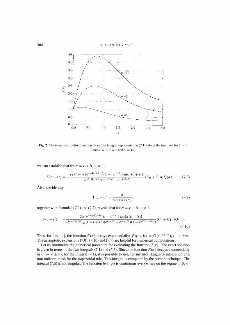
Fig. 2 The stress distribution functionf (x) (the integral representation (7.1)) along the interface forλ = π

andα = 1, α = 5 andα = 10

we can establish that forσ = c + i t , t � 1,

F(c + i t) = − iχ(t − ic)eπ/4(−t+ic)(1 + ie−π t ) tan{π(c + i t)}λ(c+i t)/2+1(e−π t/2 − e−πci/2)

(C0 + C1η)Q(σ ). (7.8)

Also, the identity

�(1 − σ) = π

sinπσ�(σ), (7.9)

together with formulae (7.2) and (7.7), reveals that forσ = c − i t , t � 1,

F(c − i t) = − 2π ie−π/4(t+ic)(i + e−π t ) tan{π(c + i t)}λ(c−i t)/2+1χ(t − i + ic)(eiπc/2 − e−π t/2)(1 − e−2π(t+ic))

(C0 + C1η)Q(σ ).

(7.10)

Thus, for large|t |, the functionF(σ ) decays exponentially:F(c + i t) = O(e−π |t |/4), t → ±∞.The asymptotic expansions (7.8), (7.10) and (7.7) are helpful for numerical computations.

Let us summarize the numerical procedure for evaluating the functionf (x). The exact solutionis given in terms of the two integrals (7.1) and (7.5). Since the functionF(σ ) decays exponentiallyasσ → c ± ∞, for the integral (7.1), it is possible to use, for instance, Laguerre integration or anon-uniform mesh for the trapezoidal rule. This integral is computed by the second technique. Theintegral (7.5) is not singular. The functionh(θ, ψ) is continuous everywhere on the segment[0, π ]


=1

=5

=10

4·5

4·0

3·5

3·0

2·5

2·0

1·5

1·0

0·5

0·00

x

f (x)

5·0

1 2 3 4 5 6 7 8

Fig. 3 The stress functionf (x): the asymptotic expansions for smallx (0 < x < 0·75) and for largex(1·8 < x < 8)—the solid curves; the exact integral representation—the dashed curves (λ = π and

α = 1, α = 5, α = 10)

and decays at the ends. To evaluate this integral we use the standard trapezoidal rule. Alternatively,one can apply Gaussian integration using Chebyshev abscissas and weights.

In Fig. 2, we plot the graphs of the stress distribution functionf (x) for λ = π for some values ofα: α = 1, α = 5 andα = 10. These graphs are in good agreement with the numerical solution byChuang (4).

Figure 3 illustrates the asymptotic expansions of the functionf (x) for small x (0 < x < 0·75)and largex (x > 1·8) for the same values ofλ andα.

The asymptotic expansions based on formulae (4.13) and (5.4) (the functionsS(x) andV (x) weretaken to be zero) give reasonable results for 0� x < 0·6 andx > 5, respectively. To evaluate thefunction�(s) and its derivatives at the pointss = 1, s = 2 ands = 1

2, s = 32 we use formulae

(3.28) and (3.23). It is important to notice that in contrast with the integral (7.4), the integral (3.23)is not singular since neither of the pointss = 1, s = 2 ands = 1

2, s = 32 belongs to the contour�.

Therefore it is not surprising that direct application of the trapezoidal rule is effective for computingthis integral.

We emphasize that the integral representation (7.1) yields excellent results for allx ∈ (ε, A) atleast within the rangeε � 10−3 andA � 1000.

The principal term of the asymptotic expansion (5.4) yields the exact formula for the stress-intensity factor at infinity

kI (α) = limx→+∞

√2πx f (x) =

√2

π

�( 12)

λ. (7.11)


By regularizing the original integro-differential equation, it is shown by Chuang (4) thatkI (α) is alinear function of the parameterα: kI (α) = aα + b with

a = 0·24√

2π = 0·6016, b = 0·30√

2π = 0·7520. (7.12)

The linear dependence of the factorkI (α) on the parameterα also follows directly from the analysisof equation (3.1). Indeed, letf (x) = f0(x) + α f1(x), where the functionsf j (x), j = 0, 1, provide

the unique solutions of equation (3.1) subject to the conditionsf (m)j (0) = δ jm , j = 0, 1; m = 0, 1

(δ jm is the Kronecker symbol). These functions are independent ofα, and thereforekI (α) = aα+b.ComputingkI (α) by formula (7.11) forα = 1, 5 and 10 confirms this conclusion and also revealsa = 0·5993,b = 0·7511. These constants are in good agreement with the numerical solution (7.12).

Thus we havekI = 0·5993α + 0·7511. It is straightforward to convert this non-dimensionalform back to its original counterpart so as to establish the functional relationship betweenK I =kI σ(0)

√L andV . To do this, we use the definition ofα from (2.17). Finally, we get

K I = 0·5993σ ′(0)L3/2 + 0·7511σ(0)L12 . (7.13)

SubstitutingL from (2.10),σ(0) from (2.11) andσ ′(0) from (2.12), we finally arrive at the followingexpression forK I as a function ofV :

K I = AV 1/12 + BV −1/12, (7.14)

whereA andB are temperature-dependent materials constants:

A =√

γ1 + γ2 − γb

R1 + R2

[(kT )

13

⟨⟨E

1 − ν2

⟩⟩Dbδb〈�〉

] 14

(7.15)

and

B =√

(γ1 + γ2 − γb)(R1 + R2)

2

(kT )

13 Dbδb〈�〉⟨⟨E

1 − ν2

⟩⟩3

− 14

. (7.16)

Equation (7.14) reduces to a quadratic equation with respect toU = V 1/12: AU2 − K I U + B = 0that has two real positive solutions. However, only one root has a physical meaning. The othersolution is meaningless since it yields higherV for lower K I and must therefore be discarded; see(4, 5).

8. Conclusion

We have presented a viable mathematical procedure to provide analytical solutions of a class ofsingular integro-differential equations that have appeared as governing equations in the diffusionalcrack growth theory. The theory was first briefly introduced in terms of its physical background,mathematical modelling and derivations of the controlling equations leading to this Cauchy-typeintegro-differential equation for the unknown stress distribution on the grain boundary ahead


of the moving crack tip. The procedure of solving this type of integral equation analyticallyinvolved the following steps. (1) Using the Mellin transformation, the equation was first convertedinto a functional-difference equation; (2) reducing this difference equation to a Riemann–Hilbertboundary-value problem on an arc; and (3) finally, analysing the coefficient of the problem, solvethe Riemann–Hilbert problem by quadratures. Also included in the solution scheme were theasymptotic solutions at smallx (that is, near the crack tip) as well as the far field (that is, asx → ∞).Since the near-tip field contains the information on the crack velocityV , and the far field is relatedto the applied stress intensityK I , this stress solution makes a connection of these two fields to yielda functional relationship betweenK I andV .

It should be emphasized that the analytical solutions obtained herein are exact. They are inexcellent agreement with the existing numerical solutions which overestimated theK I values byapproximately 0·3 per cent. This closed-form solution which pertains to steady-state creep crackgrowth is useful as a limiting asymptotic value when time approaches infinity in a more general time-dependent crack-growth problem in the transient creep regime. We leave this interesting problemfor future research.

Acknowledgement

The support of the first author by EPSRC through contract GR/R23381/01 is gratefullyacknowledged. Part of the work was implemented during a research visit he made to the MaxPlanck Institute for Metals Research (Stuttgart).

References

1. H. Riedel,Fracture at High Temperatures (Springer, Berlin 1987).2. M. F. Ashby and L. M. Brown,Perspectives in Creep Fracture (Pergamon Press, Oxford 1983).3. T.-J. Chuang, K. I. Kagawa, J. R. Rice and L. B. Sills, Non-equilibrium models for diffusive

cavitation of graininterfaces,Acta Metallurgica 27 (1979) 265–284.4. , A diffusive crack-growth model for creep fracture,J. American Ceramic Soc. 65 (1982)

93–103.5. , J.-L. Chu and S. Lee, Diffusive crack growth at a bimaterial interface,J. Appl. Mech. 63

(1996) 796–803.6. Y. A. Antipov and H. Gao, Exact solution of integro-differential equations of diffusion along

agrain boundary,Quart. Jl Mech. Appl. Math. 53 (2000) 545–674.7. A. H. England, A crack between dissimilar media,J. Appl. Mech. 32 (1965) 400–402.8. T.-J. Chuang and J. R. Rice, The shape of intergranular creep cracks growing by

surface diffusion,Acta Metallurgica 21 (1973) 1625–1628.9. F. D. Gakhov,Boundary Value Problems (Pergamon Press, Oxford 1966).

10. Jahnke, Emde and Losch,Tables of Higher Functions (Teubner, Stuttgart 1966).

APPENDIXGeneral case

In the text of this paper, we have discussed the solution to the integral equation (3.1) for a range of physicallyrelevant parameters. However, the method of analysis we presented has no limitations with respect to theparameters chosen. Here we give a general discussion of the solutions to (3.1) for different parameter rangesin case similar problems might arise in other applications.


We have solved the integro-differential equation (3.1) for positiveλ andβ = 12. It becomes evident that if

| f (x)| � Cx−β , x → ∞ for all β ∈ (0, 12], then| f (x)| � Cx− 1

2 , x → ∞. Section 3 implies that in the class0 < β � 1

2, for λ > 0, equation (3.1) has two linearly independent solutions. The general solution possessestwo arbitrary constants fixed by the conditions (3.2). Forx → 0 andx → ∞ we have obtained

f (x) = 1 + αx + O(x2 log x), x → 0,

f (x) = �( 12)

λπx− 1

2 + O(x−3/2), x → ∞. (A.1)

Consider now the next class12 < β � 1 and as beforeλ > 0. In this class, the parameterc = Re(s) in formula(3.3) is defined in the range12 < c < 1. We factorize tanπσ as follows:

tanπσ = − cotπσ

4K0(σ ), ind K0(σ ) = 1

2π[argK0(σ )]� = 0, (A.2)

and introduce the new function

�0(s) = λs/2

�(s)cos

πs

4�(s). (A.3)

By using the identity

− cotπσ

4= cos1

4πσ

cos14π(σ + 2)

(A.4)

we arrive at the problem (3.13). In contrast with the function�0(s) from section 3, the function (A.3) mustsatisfy the additional condition�0(2) = 0. This is becauses = 2 ∈ and�(s) is analytic in the strip . Bythe approach of section 3 we get

�(s) = − (1 + i)�(s) cos{ 12π( 1

2 + s − c)}Q(s)√2λs/2 cos1

4πs(C0 + C1w). (A.5)

However, the constantsC0, C1 are not arbitrary and are linked by

C0 = −iC1 tan{ 12π( 1

2 − c)}. (A.6)

Thus, equation (3.1) has only one non-trivial solution. Sinces = 12 ∈ , and the first pole of the integrand in

(4.1) in the strip 1 is s = 32, the function f (x) decays at infinity as

f (x) ∼ �(32)

πλx−3/2, x → ∞. (A.7)

This means that the solution meets the requirement| f (x)| � Cx−β , x → ∞, β ∈ ( 12, 1]. For x → 0,

f (x) ∼ −�(2) + x�(1).Next, analyse the class 1< β � 3

2 (1 < c < 32). We use the factorization (3.12), (3.14). The solution with

two arbitrary constants is defined by (3.28). At infinity, the asymptotics of the functionf (x) is given by (A.7).However, at the pointx = 0, its first derivative has the logarithmic singularity

f (x) = −�(2) + O(x log x), x → 0. (A.8)

This occurs because now the points = −1 ∈ −2, and it is a pole of the second order for the first integrand in(4.7). The fact thatf ′(x) = O(log x), x → 0, makes it impossible to employ the second condition in (3.2).

If 32 < β � 2 (3

2 < c < 2), the factorization (A.2) is applied and the solution is described by (A.5). Again,sinces = 2 ∈ is a zero of the function�0(s), by the same argument as in the case1

2 < β � 1, there is onlyone solution to equation (3.1). Its behaviour atx = 0 is given by (A.8). At infinity,

f (x) ∼ �(52)

πλx− 5

2 , x → ∞. (A.9)


For 2< β � 52 (2 < c < 5

2), the factorization of the functionK (σ ) is given by (A.2), (A.4). However, now,the points = 2 is outside the strip (the next zeros = 6 does not belong to the strip either). The generalsolution possesses two arbitrary constants and the previous formula (A.9) is still valid for this case. Atx = 0,the solution has the logarithmic singularity:f (x) = O(log x).

In the class52 < β � 3, we return to the original factorization (3.12), (3.14). Sinces = 4 ∈ ( 5

2 < c < 3)we should not expect two arbitrary constants. By the condition�0(4) = 0 one of the constantsC0, C1 is fixed,and by the same argument as in the previous case

f (x) = O(log x), x → 0, and f (x) = O(x− 72 ), x → ∞. (A.10)

Wenote that forβ > 3, in general, the solutionf (x) has a non-integrable singularity atx = 0. For instance,if 3 < β � 7

2, then f (x) = O(1/x). However, in this case, by an appropriate choice of one of the two arbitraryconstants, it is possible to remove this singularity.

So far we studied the caseλ > 0. Let nowλ < 0. If 0 < β � 12, then we need to factorize the function

− tanπσ :− tanπσ = cos1

4π(σ + 2)

cos14πσ

K0(σ ), ind K0(σ ) = 0. (A.11)

Therefore, instead of dealing with the function (3.14) we get

�0(s) = λs/2�(s)

�(s) cos14πs

. (A.12)

The function�0(s) admits a pole at the points = 2 ∈ . The scheme of section 3 yields the followingrelations for the integersp, q andκ:

−34 < p < −1

4 − κ, q = −1 − p − κ. (A.13)

The above inequality impliesκ = −1 and p = q = 0. Because of the poles = 2 of the functionϕ(w), thesolution to the Riemann–Hilbert problem (3.19) is not trivial and has one arbitrary constant:

ϕ(w) = C∗eY (w)

w − w0, (A.14)

wherew0 = i tan{ 12π( 1

2 − c)}. Therefore, the integro-differential equation (3.1) has only one solution. Asx → 0, f (x) ∼ −�(2) + x�(1), and asx → ∞, the function f (x) has the asymptotics (A.1).

In the next class12 < β � 1, we get

− tanπσ = sin 14π(σ + 2)

sin 14πσ

K0(σ ), ind K0(σ ) = 0, (A.15)

and

�0(s) = λs/2�(s)

�(s) sin 14πs

. (A.16)

It is obvious that the function�0(s) is free of poles in the strip and by the above argument, the correspondingequation (3.13) has the trivial solution only. Thus,f (x) ≡ 0.

Let us analyse the other cases. For 1< β � 32 (1 < c < 3

2), we use formulae (A.11), (A.12). The function�0(s) has a simple pole ats = 2 ∈ . The solution is defined uniquely up to an arbitrary constant factor anddisplays the following behaviour at the singular points:

f (x) = C ′ + C ′′x log x, x → 0; f (x) = O(x−3/2), x → ∞, (A.17)

whereC ′, C ′′ are constants.


If 32 < β � 2 (3

2 < c < 2), we introduce the auxiliary function (A.16) and, as in the case12 < β � 1,

f (x) ≡ 0.For 2< β � 5

2 (2 < c < 52), we use the factorization (A.15). Clearly, the function (A.16) has a simple pole

at the points = 4. This circumstance remedies the situation, the solution has one arbitrary constant and it isgiven by (A.14). At the singular points, its behaviour is described by (A.10).

Wenow state the final result.

THEOREM 1. Let f (x) ∈ H[b, B] for all b, B such that 0 < b < B < ∞ and, in addition, | f (x)| � Cx−β

as x → ∞, where C, β are positive constants. Let λ > 0 and k = 0, 1, 2, . . . . Then the integro-differentialequation

f ′′(x) = λ

π

∞∫0

f (t)dt

x − t, 0 < x < ∞, (A.18)

has two linearly independent solutions for k < β � k + 12 , and at infinity, f (x) = O(x−k− 1

2 ).If k + 1

2 < β � k + 1, equation (A.18) is solvable uniquely (up to an arbitrary constant factor), and

f (x) = O(x−k− 32 ), x → ∞. For 0 < β � 3 as x → 0, the function f (x) behaves as follows:

f (x) ∼

C ′0 + C ′′

0 x, 0 < β � 1,

C ′1 + C ′′

1 x log x, 1 < β � 2,

C ′2 log x + C ′′

2 , 2 < β � 3,

x → 0, (A.19)

where C ′k , C ′′

k (k = 0, 1, 2) are constants. For β > 3, the solution is non-integrable at x = 0.Let λ < 0. For k < β � k + 1

2 equation (A.18) has only one non-trivial solution which has the sameasymptotic properties at x = 0 and at infinity as in the case λ > 0.

For k + 12 < β � k + 1, equation (A.18) has the trivial solution only.

on the integro-differential equation associated with ...yantipov/antgaojerry.pdf · on the...

Documents