on the macroeconomic determinants of the housing market in
TRANSCRIPT
iii
On the macroeconomic determinants of the
housing market in Greece: A VECM approach
Theodore Panagiotidis# and Panagiotis Printzis*
ABSTRACT
This study examines the role of the housing market in the Greek
economy. We review the literature and assess the interdependence
between the housing price index and its macroeconomic determinants
within a VECM framework. An equilibrium relationship exists and in the
long run the retail sector and mortgage loans emerge as the most
important variables for housing. The dynamic analysis shows that the
mortgage loans followed by retail trade are the variables with the most
explanatory power for the variation of the houses price index.
Keywords: Housing Market · Greece · VECM · impulse response function ·
Granger causality
# Theodore Panagiotidis, Department of Economics, University of Macedonia, 156 Egnatia
street, 54006 Thessaloniki, Greece, [email protected] * Panagiotis Printzis, Department of Business Administration, University of Macedonia,
Thessaloniki, Greece, [email protected]

iv

1
On the macroeconomic determinants of the
housing market in Greece: A VECM approach
1. Introduction
Housing is considered to be the most valuable asset of a household and
a fundamental part of its portfolio. It provides positive externalities in
terms of social environment, public health and economic development.
The literature discounted for a long time the interaction between the
housing market and the macroeconomy by putting housing next to other
consumption goods (Leung, 2004). The recent US subprime crisis and the
subsequent collapse of the housing market revived the focus on the
housing market.
The recession and the collapse of the Greek housing market created
chain reaction effects on most sectors of the Greek economy raising the
question whether house prices reflected fundamentals. We examine the
key macroeconomic determinants by employing a two stage Vector Error
Correction Model (VECM) that takes into account exogenous variables to
gauge the short and the long run dynamics. The direction of causality
and the long-term relation between housing prices and the other
macroeconomic factors will be investigated.
The paper is organized as follows: Sections 2 discusses homeownership,
housing wealth and the financial crisis. Section 3 reviews the main
macroeconomic determinants of the housing market. Section 4 focuses
on the Greek housing market while chapter 5 presents the empirical
results. The last section draws conclusions and provides suggestions for
further research.

2
2. Background
2.1. Homeownership
The encouragement of homeownership has been a key government
policy. Its benefits and costs are still of interest to researchers (Phang,
2010). Atterhog (2005) depicts three main advantages of owning a
house: (i) private dwellings are usually of bigger size and better quality
than these of non-private property, (ii) due to the role of long-term
investment it could lead to wealth accumulation, (iii) it cultivates self-
esteem and it creates positive social externalities. Regarding the
disadvantages, the most important factor is the immobility (which could
lead to higher unemployment, Oswald 1999) and the user cost of
housing (Hickman, 2010). Glaeser and Shapiro (2002) argues that owners
desire for keeping their property value up, causing cartel and artificial
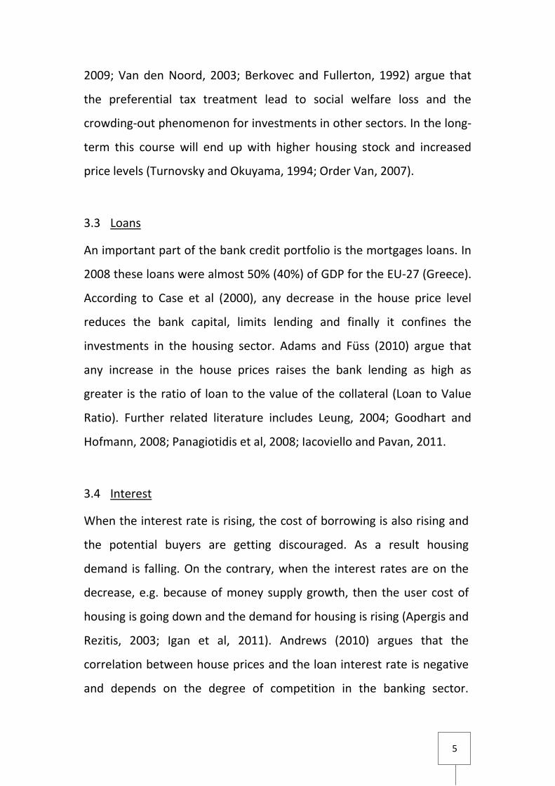
inflation actions in order to control the housing supply. Figure 1 depicts
the homeownership indices for the EU-15 countries. Greece, Spain and
Ireland emerge as champions on the one side of the scale whereas
Germany and Switzerland appear on the other.
(Please see Appendix for Figure 1)
2.2. Housing Wealth
The term housing wealth refers to the market value of all the assets or
capital stock of the residential sector in a country, rented or owned
(Iacoviello, 2011a, b). Housing wealth is connected with a household’s
income (Mirrlees et al, 2010). At the end of 2008 housing wealth in the
USA represented half of the total household wealth (Iacoviello, 2011a).

3
The same time in the Eurozone the net housing wealth represented the
60% of total wealth (ECB, 2009). Housing wealth is linked to
consumption and (non) housing investment (Case et al, 2013).
2.3. Housing market and the financial crisis
In addition to the key macroeconomic and financial factors responsible
for the crisis, fundamental was the role of housing in the change of the
consumption behavior given that is used as a collateral in most of the
cases. In some countries (for example USA and Spain) the role of the
housing sector was more active, multiplying the weight of the other
macroeconomic determinants while in others, as Greece, the housing
market wasn’t one of the main causes of the financial crisis (Hardouvelis,
2009). Ireland, Spain and Greece were the EU countries with the highest
homeownership ratio and the highest increase in house prices.
(Please see Appendix for Figure 1)
3. Housing Market and the Macroeconomic Determinants
The double role of the housing market, as a consumption good and as an
investment, has been acknowledged in the literature (Leung, 2004).
Hilbers et al (2008) classifies policies in four types; fiscal (for rents and
income), monetary (for interest rates), structural (supply and demand
for housing) and prudential (for the financing of the housing market).
3.1 GDP Income
The strong relationship between GDP, income and the housing market
has been examined in the literature. Iacoviello and Neri (2008) examine

4
the response of GDP to housing market fluctuations and Mikhed and
Zemcik (2009) concluded that in USA a decline in home prices affected
negatively the consumption and GDP. Adams and Füss (2010) noticed
that the GDP growth has an increasing impact on the housing market.
Tsatsaronis and Zhu (2004) using data from 17 industrialized countries
and through variance decomposition concluded that the long-term
contribution of GDP doesn’t exceed the 10% of the total variation of
housing price. Many studies (Davis and Heathcote, 2003; Goodhart and
Hofmann, 2008; Madsen, 2012) agree that a strong short-term
relationship exist between housing market and GDP. However Madsen
(2012) indicates that in the long term this nexus becomes weak. Turning
on the Greek economy, Merikas et al (2010) found a bidirectional
causality with a strong impact of housing investment on the economy
growth.
3.2 Taxation
There are two main reasons why government taxes residential property.
Firstly, it taxes it because of the high market value of the housing stock
and secondly because of the immobility and durability of housing that
makes it difficult to avoid taxation (Leung, 2004). However, the taxation
policy in many countries used to be favorable for homeowners. Most
Eurozone governments encourage housing investments either by
subsidizing or through tax deductions (ECB, 2009; Andrews, 2010).
Poterba (1992) following a user cost approach underlines the
importance of imputed rent taxation and of other residential taxes
which may lead to distortions in the housing market. Other studies
(Skinner, 1996; Gervais, 2002; Feldstein, 1982; Bellettini and Taddei,
5
2009; Van den Noord, 2003; Berkovec and Fullerton, 1992) argue that
the preferential tax treatment lead to social welfare loss and the
crowding-out phenomenon for investments in other sectors. In the long-
term this course will end up with higher housing stock and increased
price levels (Turnovsky and Okuyama, 1994; Order Van, 2007).
3.3 Loans
An important part of the bank credit portfolio is the mortgages loans. In
2008 these loans were almost 50% (40%) of GDP for the EU-27 (Greece).
According to Case et al (2000), any decrease in the house price level
reduces the bank capital, limits lending and finally it confines the
investments in the housing sector. Adams and Füss (2010) argue that
any increase in the house prices raises the bank lending as high as
greater is the ratio of loan to the value of the collateral (Loan to Value
Ratio). Further related literature includes Leung, 2004; Goodhart and
Hofmann, 2008; Panagiotidis et al, 2008; Iacoviello and Pavan, 2011.
3.4 Interest
When the interest rate is rising, the cost of borrowing is also rising and
the potential buyers are getting discouraged. As a result housing
demand is falling. On the contrary, when the interest rates are on the
decrease, e.g. because of money supply growth, then the user cost of
housing is going down and the demand for housing is rising (Apergis and
Rezitis, 2003; Igan et al, 2011). Andrews (2010) argues that the
correlation between house prices and the loan interest rate is negative
and depends on the degree of competition in the banking sector.

6
Frederic (2007) detects six direct and indirect ways in which the rate is
affecting the housing market: directly on the user cost of capital, on the
expectations for the future movements of prices and on the housing
supply; indirectly through housing wealth changes and credit-channel
effects on consumption and on demand. Jud and Winkler (2002) and
Painter and Redfearn (2002) argue that the influence of houses prices
on interest rates is of minor importance while others that the interest
rate is one of the most crucial macroeconomic factors of housing
(Tsatsaronis and Zhu, 2004; Assenmacher-Wesche and Gerlach, 2008;
Iacoviello, 2005; Iacoviello and Pavan, 2011; Goodhart and Hofmann,
2008; Zan and Wang, 2012).
3.5 Inflation
Kearl (1979) examined the inflationary environment and concluded that
in the case of false anticipation relative housing prices are affected.
Similarly, Follain (1981) and Feldstein (1992) infer this negative effect of
inflation on demand and on housing investments while Andrews (2010)
detect upward trends of housing prices after change of inflation in both
directions. On the other hand, Nielsen and Sorensen (1994) find that an
increasing inflation generates housing investment motives because of
the decreasing real user cost after taxes. All in all, there are discordant
views concerning the actual effect of inflation on housing market
(Manchester, 1987; Berkovec and Fullerton, 1989; Madsen, 2012;
Apergis and Rezitis, 2003; Tsatsaronis and Zhu, 2004; Bork and Muller,
2012).

7
3.6 Employment
Employment and household income are important factors (see Lerbs
2011; Giussani et al, 1992; Baffoe-Bonnie, 1998). Smith and Tesarek
(1991) examined the effect of a real estate activity decrease and found
that the latter leads to a decreased employment growth rate. Schnure
(2005) concludes that an unemployment rate percentage increase of
one unit leads to housing price decrease of 1%. Blanchflower and
Oswald (2013) and Oswald (1999) connect the labour mobility and the
home ownership rate and find evidence of negative externalities of the
housing market on the labour market. They argue that a home-
ownership rate increase affects labour mobility and leads to an
unemployment rise.
3.7 Demographics
Mankiw and Weil (1989) were the first to study the relationship
between demographics and the housing market. An increase in the
number of newborns (baby booms) has a small short-term effect on the
housing market but it increases demand for new houses twenty years
later. A decrease in the number of births or an increase in the average
age of population has a strong influence on demand and on the housing
prices.
4. The Greek Housing Market
There is an old dictum in Greece saying “No one lost his money buying
land”. The construction sector (specially housing) had been a pillar of the
Greek economy, strongly connected with many other sectors (up to

8
2009). Hardouvelis (2009) argues that investing in the housing market
was for the Greek household a form of saving. Homeownership rate
reaches 73.2% (Fig.1) while 81.5% of the Greek household assets are
related to housing. The housing investments reached their peak in 2006
representing 11.8% of GDP (Sampaniotis and Hardouvelis, 2012).
Davrakakis and Hardouvelis (2006) draw the following conclusions for
the Greek household behavior before 2009: (i) in the urban areas two
out of three dwellings are home owned, (ii) two thirds of the new buyers
were ex-renters while half of them had already a private property, (iii) in
the years 2004 & 2005 the mortgage interest rates were on a decrease
while the rents were rising. From 2006 to 2010 homeownership was
rising by 3.5% per year, (iv) eight out of ten households expected house
prices to increase for the next year as well as for the next four years, (v)
the Greek households were filled with optimism about the housing
market future and the 78% of the sample rated it as a secure
investment, (vi) housing supply was inelastic since 90% of the
respondents weren’t intended to sell their home, although the prices
were continuously rising.
4.1 Macroeconomic Determinants of the Housing Market in Greece
The main reasons for the price rise of the period 1997-2002 were the
deregulation of the bank sector, the convergence of the Greek economy
with the rest of the eurozone, the prosperous macroeconomic
environment, the inflation decline and finally the loan interest rates
decrease (Simigiannis and Hondroyiannis, 2009).

9
Simigiannis and Hondroyiannis (2009) examine whether a bubble was
present by applying the user cost model. No evidence emerged of an
increased price to rent ratio or that the housing prices were
overestimated. The same holds when using the McQuinn and O'Reilly
(2006, 2007) model.
Apergis and Rezitis (2003) analyzed the dynamic effects of the
macroeconomic variables on the housing prices in Greece. Their findings
suggest that the housing prices respond to the examined
macroeconomic variables (interest, inflation, employment, money
supply). Interest rates followed by inflation and the employment rate
were found to be the most important while money supply were not
found to be significant. Brissimis and Vlassopoulos (2007) examined the
connection between mortgages and housing prices in Greece and
couldn’t find a long term causal relationship from mortgages to prices,
although in the short-run evidence of a bi-directional relationship was
found. Merikas et al (2010) developed an equilibrium model for the
Greek housing market and concluded that construction and the labour
cost have a positive effect on the house prices while interest rates and
the non-construction investments negative. The latter is accordant with
the crowding-out effect when the rest of the economy is deprived of
investment funds. Finally, Katrakilidis and Trachanas (2012) using a non-
linear cointegration model for the period 1999-2011 found asymmetric
long-term effects of CPI and industrial production on the housing prices.

10
4.2 The causes of the crisis in the Greek Housing Market
According to Alpha Bank (2012, 2013) the main causes of the crisis are:
(i) the excessive demand of dwellings and houses, the increasing stock
and the fall of the demand, (ii) lack of liquidity in the Greek economy,
(iii) lack of positive prospects for the future of the housing market, (iv)
the high unemployment rate, (v) the general adverse economic
environment in Greece and (vi) the excessive tax burdens of the private
property.
Table 2 summarises the literature on the Greek housing market.
Please see Appendix for Table 2
5. Empirical Analysis
5.1 Variables and Data
The empirical analysis of the Greek Housing Market employs monthly
data for the period 1997:M1 to 2013:M12. Following the literature we
have focused on the following variables: House Price Index (HPI),
Consumer Price Index (CPI), Industrial Production Index (IP), volume of
Retail trade (RETAIL), loan interest rate (INTEREST), annual growth rate
of mortgages (MORTGAGE), money supply growth rate M1 (M1) and the
Unemployment rate (UNEMPL)1.
The quarterly data set for the HPI is provided by the Bank of Greece
(BoG) and refers to the urban areas and covers the time period 1997-
2013 (the frequency conversion was done in EViews). The interest rate is
1 All logged unless they are growth rates.

11
the bank interest rate on loans from the domestic credit institutions to
non- financial corporations (BoG, 2012). This is used as a proxy for the
mortgage interest rates (the availability of this series is limited) and their
correlation coefficient for the overlapping period is r=0.922. The interest
rate is the nominal one to take into account the money illusion effect.
The other factors, CPI, RETAIL and IP (excluding the construction sector),
were obtained from the OECD and the mortgage flows and the money
supply M1 growth rate were obtained from the BoG. All the variables
were seasonally adjusted nominal values (original or using U.S. Census
Bureau's X12 seasonal adjustment method). Table 3 presents the
descriptive statistics.
Please see Appendix for Table 3
5.2 VECM Model
We start the analysis with the unit root tests. Table 4 presents the
Phillips-Perron test, (Phillips and Perron, 1988) and the Unit Root Test
with Structural Break (Saikkonen and Lutkepohl, 2002; Lanne et al,
2002) and all the variables appear to be I(1). The cointegration test is
based on Johansen (1995). The Akaike information criteria (AIC)
determines the lag order. The results are presented in Table 5. The trace
test indicates the presence of one cointegration vector at the 5% level
of significance.

12
We employ a two stage estimation procedure discussed in Lütkepohl
and Krätzig (2004) that allows us to account for the exogenous
variables2. This approach requires estimation in two stages. In the first
stage, the cointegration matrix has to be estimated. All exogenous
variables are eliminated from the model for performing this step (S2S
estimator). In the second stage the exogenous variables can be
accounted for and OLS for each individual equation is used. The error
correction model includes a linear deterministic part. Money supply M1,
the unemployment rate and the interest rate are treated as exogenous
and enter in the short-term relationship but not in the long-run. The
estimated equation can be written as:
(1)
where: yt is the vector of (1) endogenous variables: , xt
the vector of exogenous variables: , Dt the vector of the
deterministic terms: , Γi the matrix of endogenous variables
coefficients, Θi the matrix of exogenous variables coefficients, C the
matrix of deterministic terms coefficients, the vector of the
2 Interest rates are set by the ECB and most likely do not reflect the economic conditions of a small
peripheral economy. Together with M1 and the unemployment rate will be treated as exogenous.

13
deterministic terms included in the cointegration relations, the
coefficients vector , β the cointegration vector, η the coefficient
matrix of the deterministic terms, α the adjustment (loading)
coefficients vector and ut the disturbance terms vector
The VECM estimates for the cointegration equation are presented in
Table 6. The long-run relationship is expressed by the following
equation (standard errors in brackets):
(2)
The results reveal that all the cointegration vector coefficients of the
model and the adjustment factor of HPI (a=-0.031) are statistically
significant. The latter implies that the error correction mechanism is
rather slow. The signs of the coefficients are in line with the literature.
All the determinants have a positive effect on housing prices. However
the IP coefficient doesn't confirm a crowding-out effect.
The cointegration relation is plotted in Figure 2:
(3)
This zˆ graph expresses the error correction term in the reference
period. In the period 2007-2013 the prices were above the level which is
defined by the market fundamentals used in the model, while in the

14
period 1997-2006 were slightly below. There is no indication of an
overestimated Greek housing market and for the first years of the crisis
(2007-2010) the housing prices show a sign of rigidity, as they fail to
adjust to the new market conditions.
Regarding the causal relationship in the long-run, Table 6 presents the
loading factors and shows that for mortgages and CPI the coefficients
are statistically insignificant, implying that a change of the housing price
index will not affect these variable, therefore the causal relationship
doesn’t have a direction from the HPI to mortgages and CPI. As a result
these variables could be treated as weakly exogenous. The same doesn’t
apply for IP and RETAIL. In the other direction any variable change has
an effect on HPI. The instantaneous and Granger causality tests are
reported in Table 7. In the short run MORTGAGE, CPI and RETAIL
Granger-cause HPI.
(Please see Appendix for Figure 2 and Tables 4, 5, 6, 7)
5.3 Dynamic Analysis
Table 8 present the results of the variance decomposition (Cholesky
decomposition). The total variance of HPI is decomposed in each period
of the forecast horizon and we measure the percentage of this variance
that each variable can explain. For the first quarters the highest

15
explanatory power is attributed to own shocks but three years after the
shock mortgages and RETAIL account for more variation (29% for both)
in houses prices than the variation which is produced by shocks to IP or
CPI (9% combined). One could argue that (i) house prices are rigid
especially in short horizons and (ii) mortgage flows and RETAIL are the
variables that can explain 29% of the HPI variation three years after the
shock.
The impulse response functions assess the dynamic behavior of the
model by examining the response of a variable after shocks to the other
variables. Generalized Impulse responses (GIRF) are employed and
bootstrapped standard errors are reported. Figure 3 reveals similar
results with the variance decomposition method. The housing price
index responds to mortgage, CPI and RETAIL shocks leveling off after 36
months from the initial shock, while shocks to IP do not cause a
statistically significant response of HPI.
Please see Appendix Figure 3 & Table 8
6. Conclusions
This study examines the long-run determinants of the housing market in
Greece by employing a two stage VECM estimation approach that allows
us to consider exogenous variables as well. First we find that an
equilibrium relationship exists. In the long-run the direction of causality
is from the mortgages and the retail trade to housing prices. In the short
run mortgages, CPI and retail Granger-cause HPI. Retail trade emerges as
the most important variable in the long-run. This is followed by
mortgage loans. Dynamic analysis (variance decomposition and GIRF)

16
reveals that the housing price index responds to mortgage, CPI and retail
trade shocks, while shocks to IP do not affect HPI in a significant way.
House prices are not affected by movements in Industrial Production.
The banking sector plays the dominant role for house prices and
increase in house prices will not be observed without an increase in
mortgage loans. Overall, mortgage loans and retail trade are the
variables to watch if you want to forecast house prices in Greece.

17
Appendix 1- Tables and Figures
Table 1: Literature Review
Title Authors Data Methodology Conclusions
House Price
Developments in
Europe : A
Comparison
Hilbers et al
(2008)
Indices: HPI, Income,
Taxation, Demographics,
Rents.
EU Countries
User cost approach
(P/R)
The model fits most of the EU countries well,
capturing the housing market developments.
Do house prices
reflect fundamentals?
Aggregate and panel
data evidence
Mikhed and
Zemcik (2009)
Housing Prices, Income,
Population, Rents,
Interest rates,
Construction Cost, Stock
market.
U.S 1980:Q2-2008:Q2 22
U.S. Metropolitan
Statistical Areas for 1978–
2007
Present value model The housing prices do not reflect
fundamentals prior to 1996 and from 1997 to
2006. They deviate from their fundamental
value and it may take decades to adjust.
Does Housing Really
Lead the Business
Cycle?
Älvarez and
Cabrero (2010)
Spanish Housing Market,
GDP components
1980:Q1 – 2008:Q4
Cross correlation
Butterworth and
Epanechnikov filters
Residential investment leads GDP. Its lead is
larger in expansions than in contractions.
There is a positive linkage between
fluctuation in housing prices and residential
construction.
Macroeconomic
determinants of
international housing
markets
Adams and
Füss (2010)
Real money supply, real
consumption, real
industrial production, real
GDP, employment, long-
term interest rates,
construction costs.
1975Q1 to 2007Q2 for 15
countries
Panel cointegration
analysis και ECM
House prices increase by 0.6% for a 1%
increase in economic activity. The divergence
from the long-term equilibrium fully adjusts
after 14 years.
Housing market
spillovers: Evidence
from an estimated
DSGE model
Iacoviello and
Neri (2008)
USA Quarterly Data
1965:I-2006:IV
Bayesian likelihood
approach Dynamic
stochastic general
equilibrium model
The slow technological progress of the
construction sector account for a large share
in the housing price upward trend. The
residential investments and the housing
prices are sensitive to demand shock and to
the monetary policy. Housing wealth affects
positively and significantly the consumption.
What drives housing
price dynamics :
cross-country
evidence
Tsatsaronis and
Zhu (2004)
GDP, Interest rates,
Spreads, Inflation, Loans
17 Industrial countries
1970-2003
SVAR (structural
vector
autoregression)
framework
Housing prices depend on inflation and credit
and they are strongly linked with the short
term interest rates.
House prices, money,
credit, and the
macroeconomy
Goodhart and
Hofmann (2008)
Quarterly data for 17
Industrial countries 1970-
2006 (money, credit,
prices, economic activity)
Fixed-effects panel
vector
autoregression
There is a multidirectional causality between
house prices, monetary variables, and the
macroeconomy. The monetary variables are
strongly linked with housing prices from 1985
to 2006. In periods of price booms the effects
of shocks to money and credit are stronger.
Housing and the
Business Cycle
Davis and
Heathcote (2003)
USA Data (Tax rate, GDP,
depreciation rate, land’s
share, population growth,
etc.). Model period of
one year
Cobb-Douglas
Equilibrium multi-
sector growth model
The volatility of the residential investment is
more than twice the volatility of business
investment. There is a positive correlation
between consumption, residential and non-
residential investment. The residential
investment leads the business cycle in
contrast with the non-residential which lags.
A behavioral model of
house prices
Madsen (2012) 18 OECD countries 1995-
2007
Repayment model of
houses price –
equilibrium model
House prices are independent of the rents.
The income elasticity of house prices reaches
one. In the long run the house prices are
driven by the acquisition costs.

18
Title Authors Data Methodology Conclusions
Real House Prices in
OECD Countries: The
Role of Demand
Shocks, Structural and
Policy Factors
Andrews (2010) Interest rates, disposable
income, CPI, housing
prices for 29 OECD
countries 1980-2005
VECM (Vector Error
Correction Model)
The housing prices rise in proportion with the
household income and with declines in the
unemployment and real interest rates.
Countries with a significant tax relief on
mortgage debt financing cost show a
tendency for demand shocks.
Taxation and Housing
Old Questions, New
Answers
Poterba (1992) USA Data 1980 -1990 User cost approach
(P/R)
The housing tax policy is associated with
distortions in the user cost of housing and in
the housing market
Housing taxation and
capital accumulation
Gervais (2002) USA data, Model period
of one year
General equilibrium
life-cycle economy
populated by
heterogeneous
agents
The favorable tax treatment of home
ownership leads to wealth loss and to
crowding-out effects. Taxation of imputed
rents or no deductible mortgage interest
rates are suggested.
Housing and the
Economy : After the
Short Run
Order Van
(2007)
Theoretical approach Growth model
Long Run
Equilibrium
Reductions of taxes on the business capital
increase the housing stock and the non-
housing consumption. Not taxing the imputed
rents increases the housing stock and
decreases the business capital which later
returns to its initial level.
Money and housing –
evidence for the euro
area and the US
Greiber and
Setzer (2007)
Euro area 1981-2006
USA 1986-2006
Quarterly data for Μ3,
GDP, housing prices,
interest rates.
VECM (Vector Error
Correction Model)
Loose monetary policy is related with the rise
of housing prices. There is a bi-directional
connection between the money and the
housing market.
Housing, credit, and
real activity cycles:
Characteristics and
comovement
Igan et al
(2011)
Australia, Austria,
Belgium, Canada,
Denmark, Finland,
France, Germany, Ireland,
Italy, Japan, the
Netherlands, New
Zealand, Norway, Spain,
Switzerland, the United
Kingdom, and the United
States 1981:Q1 to
2006:Q4
Generalized dynamic
factor model
(GDFM)
In the long run the housing price cycles lead
the credit and the real activity while in the
short run it depends on the country.
Housing and Debt
Over the Life Cycle
and Over the Business
Cycle
Iacoviello and
Pavan (2011)
U.S Economy, 1952-2010 Quantitative general
equilibrium model
In high leverage conditions the housing
market responds more and it is more
vulnerable to negative shocks than positive.
(Nonlinearity)
On the Relationship
between Credit and
Asset Prices
Panagiotidis et al
(2008)
UK & US 1964Q4-
2004Q1. Data: GDP,
mortgages, housing
prices, stock market
VECM (Vector Error
Correction Model)
Existence of a stable house price model in the
UK and of a stable stock prices model in US.
Both countries are characterized by a larger
effect of housing prices compared to the
effect of stock prices.
The Role of Interest
Rates in Influencing
Long-Run
Homeownership
Rates
Painter and
Redfearn (2002)
Quarterly data for USA
1965-1999. (interests,
prices, income,
demographics etc)
VECM (Vector Error
Correction Model)
Short term changes in income or interest
rates do not affect the home ownership rate,
Interest rates show short run impacts on
housing starts. In the long run the highest
explanatory power over home ownership rate
belongs to the demographics and to the rising
income.
Financial Structure
and the Impact of
Monetary Policy on
Asset Prices
Assenmacher-
Wesche and
Gerlach (2008)
CPI, GDP, interest rates,
prices, stock market index
for 17 countries 1986 -
2006
VAR models for
individual countries
& panel VAR
There is a large influence of the monetary
policy over the residential property prices. An
interest rate increase of 2,5% decreases GDP
by 1,25% and the property prices by 3,75% .
House Prices and
Interest Rates: A
Theoretical Analysis
Guler, and Arslan
(2010)
Real Interest rates &
Housing prices
Τwo-period
overlapping-
generations model
populated
High or low housing stock in different periods
(effective housing supply) has an ambiguous
effect on the housing price behavior in
response to fluctuations in interest rates.

19
Title Authors Data Methodology Conclusions
Empirical evidence on
the reaction speeds of
housing prices and
sales to demand
shocks
Oikarinen
(2012)
Housing price, Sales
volume, Aggregate
income, Loan-to-income
ratio, User cost %,
Housing stock for Finland
1988-2008
VECM (Vector Error
Correction Model)
The prices respond slower to demand shocks
than the sales do. The sales volume can be
used as an indicator of demand’s change and
as a predictor of house prices movements.
Money Illusion and
Housing Frenzies
Brunnermeier and
Julliard (2008)
U.K. housing market
(1966:Q2–2004:Q4)
Vector
Autoregression
(VAR) approach
It’s the nominal interest rate and not the real
which affects the housing price to rent ratio.
A large share of the variation of the mispricing
is due to movements in inflation.
The Long-Run
Relationship between
House Prices and
Rents
Gallin (2008) USA 1970:Q -2003:Q4
1970:Q1 - 2001:Q4
P/R ratio
Campbell and
Shiller’s (2001)
Mark’s (1995)
The P/R ratio is a measure of valuation of the
housing market and high values indicate a
sign of a “bubble”. However it can’t predict
precisely the direction, the time and the value
of the housing prices.
The Dynamic Impact
of Macroeconomic
Aggregates on
Housing Prices and
Stock of Houses : A
National and Regional
Analysis (1998)
Baffoe-Bonnie
(1998)
USA 1973:1-1994:4
(housing stock, prices,
interest rates, CPI,
employment, money
supply)
Vector
Autoregression
(VAR)
The housing market is sensitive to
fluctuations in the employment growth rates
and interest rates at national and regional
levels.
Does housing drive
state-level job
growth? Building
permits and
consumer
expectations forecast
a state’s economic
activity (2012)
Strauss (2012) USA 1969:1-2010:4 ARDL model The number of building permits can predict
the growth of the construction activity, is a
sign of future employment growth and it
leads housing prices and wealth.
Housing price
volatility and its
determinants
Lee (2009) Quarterly data (prices,
CPI, income, population,
interests, unemployment)
for Australia 1987:Q4 -
2007:Q4.
Εxponential-
generalized
autoregressive
conditional
Heteroskedasticity
(EGARCH) model
Volatility clustering effects and asymmetric
shocks were found in many cities. Inflation is
the main determinant of housing price
volatility.
The baby boom, the
baby bust, and the
housing market
Mankiw and
Weil (1989)
Στοιχεία ΗΠΑ 1947-1987 User cost approach
(P/R)
There are no immediate effects on the
housing market after an increase in the
number of births, but after 20 years the
demand increases. The number of births is a
leading indicator of future changes in the
housing demand.
How Long Do Housing
Cycles Last ? A
Duration Analysis for
19 OECD Countries
Bracke (2011) Quarterly data 1970:1-
2010:1 for 19 OECD
countries
Linear Probability
Model (LPM)
Upturns last longer than downturns. An
increasing duration of the upturns makes
them more likely to end Thus an overheated
economy faces the potential to enter a
downturn.
Wealth Effects
Revisited 1975-2012
Case, Karl E.,
Quigley, John M.
and Shiller, Robert
J. (2013)
Quarterly data from 1795
to 2012 for a panel of U.S
State
OLS and ECM
models
There is a large effect of housing wealth on
housing consumption, larger than the effect
of stock market. When housing prices
increase the household spending increases,
when they decrease they affect negatively the
household consumption.

20
Table 2: Literature Review of the Greek Housing Market
Title Authors Data Methodology Conclusions
Housing prices and
macroeconomic
factors in Greece:
prospects within the
EMU
Apergis and Rezitis
(2003)
Quarterly data of
interest, inflation,
employment, money
supply, housing prices for
Greece 1981-1999.
VECM (Vector Error
Correction Model)
The prices respond to the macroeconomic
variables. The highest explanatory power
belongs to the interest rates followed by
inflation and employment whereas lower is
the contribution of the money supply.
Τιµές κατοικιών: Η
πρόσφατη ελληνική
εμπειρία
Simigiannis and
Hondroyiannis
(2009)
Quarterly data for Greece
1994:Q1-2007:Q4
User Cost
Fully Modified
Ordinary Least
Squares
ECM (Error
Correction Model)
There are no signs of housing overpricing in
the recent past. The elasticity of housing price
to mortgage value comes to 0,78. The causal
relationship between loans and housing
prices appear to be bidirectional.
The interaction
between mortgage
financing and housing
prices in Greece
Brissimis and
Vlassopoulos
(2007)
Quarterly data of GDP,
interests, mortgages, for
Greece 1993:Q4-2005:Q2
VECM (Vector Error
Correction Model)
There are no results of a long term causal
relationship from mortgages to the housing
prices while in the short run these is evidence
of a bidirectional relation between the two
variables.
Explaining house price
changes in Greece
Merikas et al
(2010)
Quarterly data for Greece
1985:Q1-2008:Q1
FDW model
VECM (Vector Error
Correction Model)
The construction and the labor cost are
affecting positively the prices whereas the
interest rates and the non-construction
production negatively (crowding out). There is
evidence of substitution between the stock
market and the housing market in Greece.
What drives housing
price dynamics in
Greece: New evidence
from asymmetric
ARDL cointegration
Katrakilidis and
Trachanas (2012)
Monthly data of prices,
CPI, industrial production
for Greece 1999:Μ1-
2011:Μ5
Αsymmetric ARDL
cointegration
methodology
Asymmetric long-term effects of CPI and IPI
on housing prices. In the short run the
asymmetric effects on the prices are
statistically significant.
Table 3: Descriptive Statistics
HPI IP MORTGAGE RETAIL CPI M1 UNEMPL INTEREST
Mean 5.218237 4.687843 19.11426 4.534164 4.484666 5.860784 12.53573 9.254345 Median 5.253439 4.735396 23.57232 4.541165 4.491741 5.900000 10.60000 7.496467
Maximum 5.570781 4.822417 40.84383 4.848116 4.706811 38.40000 27.70000 19.70000
Minimum 4.561120 4.431090 -3.721505 4.252772 4.201898 -17.30000 7.400000 5.722567
Std. Dev. 0.289692 0.111782 13.53631 0.165307 0.152706 10.90306 5.376480 3.902506 Skewness -0.682336 -0.910458 -0.534905 0.060629 -0.133081 0.093267 1.845845 1.479799
Kurtosis 2.360679 2.524601 1.931786 1.844874 1.754847 3.025883 5.091084 3.669649
Jarque-bera
19.30400
30.10477
19.42740
11.46667
13.78061
0.301455
153.0103
78.26500
Probability 0.000064 0.000000 0.000060 0.003236 0.001018 0.860082 0.000000 0.000000
Sum
1064.520
956.3199
3899.308
924.9694
914.8718
1195.600
2557.289
1887.886
Sum Sq. Dev. 17.03602 2.536542 37196.03 5.547262 4.733797 24131.97 5868.028 3091.599
Observation
204
204
204
204
204
204
204
204

21
Table 4: Unit Roots and Stationarity Tests
Variable
Phillips-Perron UR Test with Str. Break Structural Breaks
Levels
Difference
Levels
Difference
Levels
Difference
HPI -3.00** -3.16** -1.34 -3.35** 2009M1 2009M1
IP -0.143 -26.62*** -1.35 -6.03*** 2008M2 2011M8
MORTGAGE -0.04 -12.05*** -1.66 -5.89*** 2001M3 2002M1
RETAIL -0.87 -18.86*** -0.87 -6.12*** 2010M4 2008M11
CPI -2.75 -13.43*** -1.05 -5.28*** 2011M9 2011M9
M1 -2.30 -15.87*** -2.09 -4.18*** 2000M3 1999M12
UNEMPL 2.01 -10.46*** -1.68 -2.83* 2004M1 2004M2
INTEREST -3.64*** -13.33*** -0.43 -5.95*** 1997M11 1997M11
Critical Value 1% -3.46 -3.46 -3.55 -3.55
Critical Value 5% -2.88 -2.88 -3.03 -3.03
Critical Value 10% -2.57 -2.57 -2.76 -2.76
Note: The UR Test with Structural Break is proposed by Saikkonen and Lutkepohl (2002); Lanne et al (2002) (Ho: unit root), Phillips-Perron test (Ho: unit root), *** (**, *) rejects the
null hypothesis at the 1% (5% and 10%) level, Phillips-Perron test includes a constant term
and the Structural Break test a constant term, a time trend and seasonal dummies.
Table 5: Johansen Cointegration Test
Ho: Rank Trace Value p-Value 90% 95% 99%
0 96.56 0.0109 84.27 88.55 96.97
1 59.55 0.1083 60.00 63.66 70.91
2 35.63 0.2230 39.73 42.77 48.87
3 21.14 0.1761 23.32 25.73 30.67
4 9.05 0.1821 10.68 12.45 16.22
Note: 1. 5 included lags (levels) based on Akaike Information Criterion, 2.
Trend and intercept included 3. Sample range: [1997 M6, 2013 M12], T = 199, 4. Critical values from Johansen (1995) and the p-values are from
Doornik (1998).
Table 6: VECM Long run coefficients - Diagnostic Tests
Cointegrating Eq: HPIt-1 IPt-1 MORTGAGEt-1 RETAILt-1 CPIt-1 CONSTANT TRENDt-1
1.000 -0.352 -0.005 -0.784 -2.582 11.346 0.003
(0.000) (0.094) (0.001) (0.055) (0.320) (1.312) (0.001)
{0.000} {0.000} {0.000} {0.000} {0.000} {0.000} {0.000}
[0.000] [-3.744] [-7.811] [-14.273] [-8.070] [8.650] [3.973]
Loading factors:
-0.031 0.205 -4.342 0.532 -0.007 (0.014) (0.093)
(3.479)
(0.103)
(0.012)
{0.032} {0.027} {0.212}
{0.000} {0.537} [-2.147] [2.209] [-1.248] [5.156] [-0.617]
ARCH-LM test (32 lags): {0.1876} {0.8572} {0.0000} {0.9604} {0.0613}
Multivariate ARCH-LM test (5 lags):
{0.4747}
LM-Type test for
autocorrelation (5 lags):
{0.0551}
Note: Standard errors in ( ), p-values in { } and t-statistics in [ ]

22
Table 7: Causality Tests from the VECM Model
Cause Variables: ∆(HPI) ∆(IP) ∆(MORTGAGE) ∆(RETAIL) ∆(CPI)
Effect Variables: ∆(IP) ∆(HPI) ∆(HPI) ∆(HPI) ∆(HPI)
∆(MORTGAGE) ∆(MORTGAGE) ∆(IP) ∆(IP) ∆(IP)
∆(RETAIL) ∆(RETAIL) ∆(RETAIL) ∆(MORTGAGE) ∆(MORTGAGE)
∆(CPI) ∆(CPI) ∆(CPI) ∆(CPI) ∆(RETAIL)
Granger Causality 0.0002* 0.1722 0.0051* 0.0122* 0.0469*
Instantaneous Causality 0.0035* 0.0658 0.0505 0.8277 0.8526
Note: only p-values are reported, Granger Test, H0: doesn’t Granger cause,
Instantaneous Test, H0: No instantaneous causality, * rejects the null hypothesis at the
5% level
Table 8: Forecast Error Variance Decomposition of HPI
FORECAST HORIZON HPI IP MORTGAGE RETAIL CPI
3 0.97 0,00 0.01 0,00 0.01 6 0.92 0,00 0.04 0.01 0.02
9 0.85 0.01 0.08 0.03 0.03 12 0.79 0.01 0.11 0.05 0.04
15 0.75 0.01 0.13 0.06 0.05
18 0.71 0.01 0.15 0.07 0.06 21 0.69 0.01 0.16 0.08 0.07
24 0.67 0.01 0.17 0.09 0.07
27 0.65 0.01 0.17 0.09 0.07 30 0.64 0.01 0.18 0.09 0.08
33 0.63 0.01 0.18 0.09 0.08
36 0.62 0.01 0.19 0.10 0.08
Note: The columns give the proportion of forecast error in HPI accounted for by each
endogenous variable
23
Fig. 1: Home Ownership Ratio
Figure 2: Cointegration Graph

24
Figure 3: Impulse Responses

25
References
Adams Z, Füss R (2010) Macroeconomic determinants of international housing
markets. Journal of Housing Economics 19(1):38 50
Alpha Bank (2012) Weekly economic reports 21/11/2012, 27/12/2012.
Economic – Markets Research Alpha Bank
Alpha Bank (2013) Weekly economic report 14/8/2013. Economic - Markets
Research Alpha Bank URL
http://www.alpha.gr/page/default.asp?la=1&id=2450
Alvarez, Luis J. and Cabrero, Alberto, (2010), Does housing really lead the
business cycle?, No 1024, Banco de España Working Papers, Banco de
España.
Andrews D (2010) Real house prices in OECD countries: The role of demand
shocks and structural and policy factors, OECD Economics Department
Working Papers, No. 831, OECD Publishing.
Apergis N, Rezitis A (2003) Housing prices and macroeconomic factors in
Greece: prospects within the EMU. Applied Economics Letters 10(9):561
565
Assenmacher-Wesche K, Gerlach S (2008) Financial structure and the impact
of monetary policy on asset prices, Swiss National Bank Working Papers
Atterhog M (2005) Importance of government policies for home ownership
rates: an international survey and analysis. Working paper no. 54, Swedish
Royal Institute of Technology
Baffoe-Bonnie J (1998) The dynamic impact of macroeconomic aggregates on
housing prices and stock of houses: a national and regional analysis. Journal
of Real Estate Finance and Economics 17(2):179- 97
Bellettini G, Taddei F (2009) Real estate prices and the importance of bequest
taxation. Working paper series no. 2577, CESifo
Berkovec J, Fullerton D (1989) The general equilibrium effects of inflation on
housing consumption and investment. American Economic Review 79:277-
282
Berkovec J, Fullerton D (1992) A general equilibrium model of housing, taxes,
and portfolio choice. Journal of Political Economy 100(2):390-429

26
Blanchflower, D G and A J Oswald (2013), “Does high home-ownership impair
the labor market?” Working Paper Series WP13-3, Peterson Institute for
International Economics
BoG (2012) Statistical data Bank of Greece. URL
http://www.bankofgreece.gr/Pages/el/Statistics/default.aspx
Bork L, Müller SV (2012) Housing price forecast ability: A factor analysis
Bracke P (2011) How long do housing cycles last? A duration analysis for 19
OECD countries. IMF Working Papers 11/231, International Monetary Fund
Brissimis NS, Vlassopoulos T (2007) The interaction between mortgage
financing and housing prices in Greece. Economic Research Department,
Special Studies Division, Bank of Greece (58)
Brunnermeier MK, Julliard C (2008) Money illusion and housing frenzies. The
Review of Financial Studies 21:135 180
Case KE, Glaeser EL, Parker JA (2000) Real estate and the macroeconomy.
Brookings Papers on Economic Activity 2000(2):119-162
Case, Karl E., Quigley, John M. and Shiller, Robert J., (2013), Wealth Effects
Revisited 1975-2012, Critical Finance Review, 2, issue 1, p. 101-128
Davis Ma, Heathcote J (2003) Housing and the business cycle. SSRN Electronic
Journal URL http://www.ssrn.com/abstract=528102
Davrakakis M, Hardouvelis G (2006) Einai ipertimimeni h agora akiniton (in
Greek). ISSN: 1790-6881, Division of Research & Forecasting, Eurobank, URL
http://www.hardouvelis.gr/FILES/PROFESSIONAL%20WORK/OikonomiaAgo
res.pdf
Doornik, J. A. (1998). Approximations to the asymptotic distributions of
cointegration tests, Journal of Economic Surveys 12: 573–593.
ECB (2009) Housing finance in the euro area. Occasional Paper Series 101
European Central Bank
Feldstein M (1982) Inflation, tax rules and accumulation of residential and
non-residential capital. Scandinavian Journal of Economics 84(2):293-311
Feldstein MS (1992) Discussion on James M. Poterba, Tax reform and the
housing market in the late 1980s: who knew what, and when did they know
it? pp 230-261
27
Follain JR (1981) Does inflation affect real behavior? The case of housing,
Southern Economic Journal 48:570-82
Frederic MS (2007) Housing and the monetary transmission mechanism.
Finance and Economics Discussion Series Divisions of Research & Statistics
and Monetary Affairs Federal Reserve Board, Washington
Gallin J (2008) The long-run relationship between house prices and rents. Real
Estate Economics 36(4):635-658
Gervais M (2002) Housing taxation and capital accumulation. Journal of
Monetary Economics 49(7):1461-1489
Giussani B, Hsai M, Tsolacos S (1992) A comparative analysis of the major
determinants of office rental values in Europe. Journal of Property
Valuation and Investment 11:157-173
Glaeser E, Shapiro J (2002) The benefits of the home mortgage interest
deduction. Discussion paper no1979 Harvard university, Massachusetts
Goodhart C, Hofmann B (2008) House prices, money, credit, and the
macroeconomy. Oxford Review of Economic Policy 24(1):180-205
Greiber C, Setzer R (2007) Money and housing, evidence for the euro area and
the US. Deutsche Bundesbank, Discussion Paper Series 1: Economic Studies,
No 12/2007
Guler, Bulent and Arslan, Yavuz, Housing Prices and Interest Rates: A
Theoretical Analysis (August 19, 2010). Available at SSRN:
http://ssrn.com/abstract=1237722
Hardouvelis AG (2009) H spoudaiotita tis agoras katoikias sthn oikonomia (in
Greek). Agores akiniton Ekseliksis kai prooptikew URL
http://www.bankofgreece.gr/Pages/
el/Statistics/realestate/realestate29_4_09.aspx
Hickman P (2010) Understanding residential mobility and immobility in
challenging neighbourhoods. Research Paper 8, CRESR, Sheffield Hallam
University
Hilbers P, Ho maister AW, Banerji A, Shi H (2008) House price developments in
Europe?: A comparison. Tech. rep., IMF Working Papers 08/211,
International Monetary Fund
Iacoviello M (2005) House prices, borrowing constraints, and monetary policy
in the business cycle. American Economic Review 95:739-764