on the mark: a theory of floating exchange rates based … · rates based on real interest...

On the Mark: A Theory of Floating ExchangeRates Based on Real Interest Differentials

By JEFFREY A. FRANKEL*

Much of the recent work on floatingexchange rates goes under the name of the"monetary" or "asset" view; the exchangerate is viewed as moving to equilibrate theinternational demand for stocks of assets,rather than the international demand forflows of goods as under the more traditionalview. But within the asset view there are twovery different approaches. These approacheshave conflicting implications in particular forthe relationship between the exchange rateand the interest rate.

The first approach might be called the"Chicago" theory because it assumes thatprices are perfectly flexible.' As a conse-quence of the flexible-price assumption,changes in the nominal interest rate reflectchanges in the expected inflation rate. Whenthe domestic interest rate rises relative to theforeign interest rate, it is because the domes-tic currency is expected to lose value throughinflation and depreciation. Demand for thedomestic currency falls relative to the foreigncurrency, which causes it to depreciateinstantly. This is a rise in the exchange rate,defined as the price of foreign currency. Thuswe get a positive relationship between theexchange rate and the nominal interest differ-ential.

The second approach might be called the"Keynesian" theory because it assumes thatprices are sticky, at least in the short run.^ As

•Assistant professor. University of California-Berke-ley. An earlier version of this paper was presented at theDecember 1977 meetings of the Econometric Society inNew York, I would like to thank Rudiger Dornbusch.Stanley Fischer, Jerry Hausman, Dale Henderson,Franco Modigliani, and George Borts for comments.

'See papers by Jacob Frenkel and by John Bilson.^The most elegant asset-view statement of the Keynes-

ian approach is by Rudiger Dornbusch {!976c), to whichthe present paper owes much. Roots lie in J. MarcusFleming and Robert Mundell (1964. 1968). They arguedthat if capital were perfectly mobile, a nonzero interestdifferential would attract a potentially infinite capitalinflow, with a large effect on the exchange rate. More

a consequence of the sticky-price assumption,changes in the nominal interest rate reflectchanges in the tightness of monetary policy.When the domestic interest rate rises relativeto the foreign rate it is because there has beena contraction in the domestic money supplyrelative to domestic money demand without amatching fall in prices. The higher interestrate at home than abroad attracts a capitalinflow, which causes the domestic currency toappreciate instantly. Thus we get a negativerelationship between the exchange rate andthe nominal interest differential.

The Chicago theory is a realistic descrip-tion when variation in the inflation differen-tial is large, as in the German hyperinflationof the 192O's to which Frenkel first applied it.The Keynesian theory is a realistic descrip-tion when variation in the inflation differen-tial is small, as in the Canadian float againstthe United States in the I950's to whichMundell first applied it. The problem is todevelop a model that is a realistic descriptionwhen variation in the inflation differential ismoderate, as it has been among the majorindustrialized countries in the 197O's.

This paper develops a model which is aversion of the asset view of the exchange rate,in that it emphasizes the role of expectationsand rapid adjustment in capita! markets. Theinnovation is that it combines the Keynesianassumption of sticky prices with the Chicagoassumption that there are secular rates ofinflation. It then turns out that the exchangerate is negatively related to the nominalinterest differential, but positively related tothe expected long-run inflation differential.The exchange rate differs from, or "over-shoots," its equilibrium value by an amount

recently. Victor Argy and Michael Porter, Jiirg Niehans,Dornbusch (I976a,b.c), Michael Mussa (1976) andPentti Kouri {I976a,b) have introduced the role ofexpectations into the Mundell-Fleming framework.

610

69 NO- 4 FRANKEL FLOATING EXCHANGE RATES 61}

which is proportional to the real interestdifferential, that is, the nominal interestdifferential minus the expected inflationdifferential. If the nominal interest differen-tial is high because money is tight, then theexchange rate lies below its equilibrium value-But if the nominal interest differential is highmerely because of a high expected inflationdifferential, then the exchange rate is equal toits equilibrium value, which over timeincreases at the rate of the inflation differen-tial.

The theory yields an equation of exchangerate determination in whieh the spot rate isexpressed as a function of the relative moneysupply, relative income level, the nominalinterest differential (with the sign hypothe-sized negative), and the expected long-runinflation differential (with the sign hypothe-sized positive). The hypothesis is readilytested, using the mark/dollar rate, against thetwo alternative hypotheses: the Chicago the-ory, which implies a positive coefficient on thenominal interest differential, and the Keynes-ian theory, which implies a zero coefficient onthe expected long-run inflation differential.

1. The Real Interest Differential Theory ofExchange Rate Determination

The theory starts with two fundamentalassumptions. The first, interest rate parity, isassociated with efficient markets in which thebonds of different countries are perfect substi-tutes:

(1) d = r - r'

where r is defined as the log of one plus thedomestic rate of interest (which is numeri-cally very elose to the actual rate of interestfor normal values) and r* is defined as the logof one plus the foreign rate of interest.^ If d is

'The rates of interest referred to are instantaneousrates per unit of time, i.e., the forces of interest. In theabsence of uncertainty {or, in the stochastic case, if theterm structures of the interest differential and theforward discount contain no risk premium), equation (1)should also hold when the rates are deJined over anyfinite interval r, since the left-hand and right-hand sideswould be equal to the expected future values of theleft-hand side and right-hand side, respectively, of (1)integrated from 0 to r.

considered to be the forward discount, definedas the log of the forward rate minus the log ofthe current spot rate, then (1) is a statementof covered (or closed) interest parity. Underperfect capital mobility, that is, in the absenceof capital controls and transactions costs,covered interest parity must hold exactly,sinee its failure would imply unexploitedopportunities for certain profits." However, dwill be defined as the expected rate of depre-ciation; then (1) represents the strongercondition of uncovered (or open) interestparity. Of course if there is no uncertainty, asin a perfect foresight economy, then theforward discount is equal to the expected rateof depreciation, and (1) follows directly. Ifthere is uncertainty and market participantsare risk averse, then the assumption that thereis no risk premium, though not precluded, is astrong one.^

The second fundamental assumption is thatthe expected rate of depreciation is a functionof the gap between the current spot rate andan equilibrium rate, and of the expectedlong-run inflation differential between thedomestic and foreign countries:

(2) = -6{e - e ) + TT - TT*

where e is the log of the spot rate; -K and IT*are the current rates of expected long-runinflation at home and abroad, respectively.(We can think of them as long-run rates ofmonetary growth that are known to thepublic.)*' The log of the equilibrium exchangerate e is defined to increase at the rate 7r - ir*in the absence of new disturbances; a moreprecise explanation will be given below. Equa-tion (2) says that in the short run theexchange rate is expected to return to its

*For evidence that the deviations from covered interestparity are smaller than transactions costs, see Frenkeland Richard Levich.

'My paper shows the conditions under which, despiterisk aversion, there is a zero risk premium in the forwardexchange rate. Briefly, the conditions are no outsidenominal assets and no correlation between the values ofcurrencies and the values of real assets.

*If there is no long-run growth of real income ortechnical change in the demand for money, then the ratesof monetary growth are T and ir*. If there is long-run realgrowth or technical change, then we would adjust themonetary growth rates before arriving at the expectedlong-run inflation rates ir and v'.

612 THE AMERICAN ECONOMIC REVIEW SEPTEMBER 1979

equilibrium value at a rate which is propor-tional to the current gap, and that in the longrun, when e = ^, it is expected to change at thelong-run rate -rr - x*. For the present, thejustification for equation (2) will be simplythat it is a reasonable form for expectations totake in an inflationary world. This claim willbe substantiated in Appendix A, after aprice-adjustment equation has been specifiedby a demonstration that (2), with a specificvalue implied for 6, follows from the assump-tions of perfect foresight (or rational expecta-tions in the stochastic case) and stability.^The rational value of 6 will be seen to becloseiy related to the speed of adjustment inthe goods market.

Combining equations (1) and (2) gives

(3) e-e--^-[{r-T)^ (r* - x*)]

We might describe the expression in bracketsas the real interest differential.** Alterna-tively, note that in the long run when e = e,vvemust have ? - r* = IT - ir*, where r and r*denote the long-run, short-term interestrates.^ Thus the expression in brackets isequal to [{r - r*) - if - ?*)], and theequation can be described intuitively asfollows. When a tight domestic monetarypoiicy causes the nominal interest differential

'Note, however, that the assumption of rational expec-tations or perfect foresight is not required for equation(2) and thus is nol required for the model,

"This would nol be quite right because the nominalinterest rates are short term while the expected inflationrates are long term. However. It does turn out, with aprice-adjustment equation such as is adopted in Appen-dix A, that e - e is proportional to the shorl-term realinterest differential [{r - Dp) - {r* - Dp*)\-

'In words, long-run equality between the nominalinterest differential and the expected inflation differen-tial follows from interest rate parity (equality betweenthe interest differential and expected depreciation) andlong-run relative purchasing power parity (equalitybetween depreciation and the inflation differential). Analternative argument is that in the long run internationalinvestment flows insure that real interest rates are equalacross countries: J — ir = r* - w*. The investmentargument is not necessary, however, nor, if used, does itpreclude the possibility of different real rates of interestin the short run, since even the most perfectly classical ofeconomies have fixed capital stocks that earn nonzeroprofits in the short run.

to rise above its long-run level, an incipientcapital inflow causes the value of the currencyto rise proportionately above its equilibriumlevel.

For a complete equation of exchange ratedetermination, it remains only to explain e.Assume that in the long run, purchasingpower parity holds:

(4) e =p -p*

where p and p* are defined as the logs of theequilibrium price levels at home and abroad,respectively.'*^

Assume also a conventional money demandequation:

(5) m = p + <t>y - \r

where m, p, and y are defined as the logs ofthe domestic money supply, price level, andoutput. A similar equation holds abroad. Letus take the difference between the two equa-tions:

(6) m - m* = p - p* +

- \{r r*)

Using bars to denote equilibrium values andremembering that in the long run, when e = e.r - r* = IT - T*, we obtain

(7) e-p^p*

^m -In* - ii>(y - y*) + \{-K - w*)

This equation illustrates the monetary theoryof the exchange rate, according to which theexchange rate is determined by the relativesupply of and demand for the two currencies.It says that in full equilibrium a givenincrease in the money supply inflates pricesand thus raises the exchange rate proportion-ately, and that an increase in income or a fallin the expected rate of inflation raises thedemand for money and thus lowers theexchange rate.

'"This assumption rules out tbe possibility of perma-nent shifts in the terms of trade and so gives essentially aone-good model. It does allow the possibility of temporaryshifts; the existence of large departures from the Law ofOne Price for international trade even in closely matchedcategories of goods has been shown in studies by PeterIsard and by Irving Kravis and Robert Lipsey.

VOL. 69 NO. 4 FRANKEL: FLOATING EXCHANGE RATES 613

Substituting (7) into (3), and assumingthat the current equilibrium money suppliesand income levels are given by their currentactual levels." we obtain a complete equationof spot rate determination:

(8) e = m - m* - <t>{y - y*)

This is the equation which is tested empiri-cally for the deutsche mark in Section III.

II. Testable Alternative Hypotheses

Equation (8) is reproduced here with anerror term:'^

(9) e = m - m* - (ftiy - y*)

+ a{r - /•*) + /3(7r - TT*) + u

where a (= —1/9) is hypothesized negativeand 13 (= 1/6 + \) is hypothesized positiveand greater than a in absolute value. Tests ofa hypothesis are always more interesting if aplausible alternative hypothesis is specified.One obvious alternative hypothesis is Dorn-busch's incarnation of the Keynesian ap-proach, in which secular inflation is not afactor. In fact the model developed in thispaper is the same as the Dornbusch model inthe special case where 5r - TT* always equalszero.'^ The testable hypothesis is ^ = 0.

Another—more conflicting—alternativehypothesis comes from the Chicago theory ofthe exchange rate attributable to Frenke! andBilson. The variant presented by Bilsonbegins with a money demand equation like

"Actual money supplies and actual income levels canboth easily be allowed to differ from their equilibriumlevels, but these extensions of the analysis are omittedhere in the interest of brevity.

'^It is not stated here where the errors come from.Probably the most likely source of errors is the moneydemand equation (5), which would bias the coefficient of(m - m*) downward if it is not constrained to be one.This possibility is discussed below.

'^See Dornbusch (1976c). The only other differencesbetween the present model and the Dornbusch model arethat the former is a two-country model, while the latter isa small-country model, and the latter uses a slightlydifferent price-adjustment equation.

(5): m - p = <}>y - \r. Subtracting theforeign version yields a relative moneydemand equation like (6): {m - m*) -(p - p*) = (fiiy - y*) - X(r - r*). Bilsonthen assumes that purchasing power parityalways holds:

(10) e = p - p* = {m - m*)

- y*) + Kr ~ r*)

An increase in the domestic interest ratelowers the demand for domestic currency andcauses a depreciation. In terms of equation(9), a, the coefficient of the nominal interestdifferential, is hypothesized to be positiverather than negative.

The interest differential (r - r*) is viewedas representing the relative expected inflationrate (TT - x*), either because internationalinvestment flows equate real rates of interest,or because interest rate parity insures that theinterest difl'erential equals expected deprecia-tion, and purchasing power parity insures thatdepreciation equals relative inflation. Thusthe expected inflation difl"erential (were itdirectly observable) could be put into (10)instead of the nominal interest difl'erential:

(11)

7r*)

In terms of equation (9), a is hypothesized tobe zero and /3 to be positive, if we use a goodproxy for (ir - 7r*). Or, more generally, thehypothesis can be represented a -i- /3 = \ > 0,a > 0. /i > 0. The relative size of a and )3would depend on how good a proxy we havefor the expected inflation difl'erential.

Indeed Frenkel begins his analysis with theassumption of a Cagan-type money demandfunction, which uses the expected inflationrate rather than the interest rate:

(12) m - p = <t>y - Xw

The assumption of purchasing power paritythen gives equation (11) directly. Frenkeluses the expected rate of depreciation asreflected in the forward discount in place ofthe unobservable expected inflation difl'eren-tial which, in well-functioning bond markets,

614

would be the same as using the nominalinterest differential.

The argument that the nominal interestdifferential is equal to the expected inflationdifferential is the same as that given in thederivation of equation (7). and indeed equa-tion (11) is identical to equation (7), exceptthat (7) is hypothesized to hold only inlong-run equilibrium while (10) is hypothe-sized to hold always.''* The Frenkel-Bilsontheory could be viewed as a special case of thereal interest differential theory where theadjustment to equilibrium is assumed instan-taneous; that is, $ is infinite, which of course isthe same as a being zero.

The theory was originally tested by Frenkelon the German 1920-23 hyperinflationduring which, it is argued, inflationary factorsswamp everything else. In particular, varia-tion in the expected inflation rate dwarfsvariation in the real interest rate in the effecton the demand for money and thus theexchange rate. The argument is convincing; itis quite likely that the hypothesis a < 0 wouldbe rejected (or the hypothesis a > 0 could notbe rejected) if (9) were estimated on hyperin-flation data. This just says that the Frenkeltheory is the relevant one in the polar casewhen the inflation differential is very highand variable, much as the Dornbusch theoryis clearly the relevant one in the polar casewhen the inflation differentia! is very low andstable.

It is the claim of the real interest differen-tial theory that it is a realistic description inan environment of moderate inflation differ-entials such as has existed in the six yearssince the beginning of generalized floating in1973, and that the alternative hypothesesbreak down in such an environment. Bilsonhas suggested and tested his theory for thisperiod, and has claimed that empirically itworks better than any alternative theoryproposed.

The various alternative hypotheses aresummarized in terms of equation (9):

•M/C REVIEW

Keynesian Model,Dornbusch (1976c):

Chicago Model, Bilson:Frenkel:

SEPTEMBER

a <a ;a =

Real Interest DifferentialModel; a <

' 0 ^>0 /3=̂ 0 15

cO 8

1979

= 0= 0

' > 0

: > 0

III. Econometric Findings

In this section the real interest differentialtheory is tested on the mark/dollar exchangerate.'^ There are several good reasons forconcentrating on this rate. The variation inthe German-American inflation differentialhas been significant, as opposed to, for exam-ple, that in the Canadian-American orGerman-Swiss differentials. The exchangeand capital markets are free from extensivegovernment intervention in Germany and theUnited States, as opposed to, for example,those in the United Kingdom or Japan. Inaddition, the size of the German and Ameri-can economies and the fact that there havebeen unexpectedly large upswings anddownswings in the mark/dollar rate make thisexchange rate the most important one toexplain.

The sample used consisted of monthlyobservations between July 1974 and February1978. The results were not greatly affected bythe choice of monetary aggregate; only thoseusing A/| are reported in Table 1. Industrialproduction indices were used in place ofnational output, since the latter is not avail-able on a monthly basis. Three-month moneymarket rates were used for the nominal inter-est differential, divided by four to convertfrom a "percent per annum" basis to a three-month basis. Two kinds of proxies for theexpected inflation differential were tried,both expressed on a three-month basis: pastinflation differentials (averaged over thepreceding year) and long-term interest differ-entials (under the rationale that the long-termreal interest rates are equal).'** The advantage

'*In view of the result, (A4) in the Appendix, that thepurchasing power parity gap is proportional to the realinterest differential, it is not surprising that a theorywhich assumes that the former is always zero should alsoassume that the latter is always zero.

"Germany is viewed as the domestic country in theeconometric equations.

'*The equality of current long-term real rates ofinterest follows from the result that in the long run theshort-term real rates are equal, and the requirement of a


TABLE 1—TEST OF REAL INTEREST DIFFERENTIAL HYPOTHESIS(Sample: July 1974-February 1978)

Technique Constant R- O.W.Number of

Observations

OLS

CORC

INST

FAIR

1.33(.10).80

(.19)1,39(.08)1.39(.12)

.87(-17).31

(-25).96

(.14).97

(-21)

- .72(.22)

- ,33(.20)

- .54(.18)

- .52(-22)

-1.55(1.94)-.259(1.96)

-4.75(1.69)

-5.40(2.04)

28.65(2,70)7,72

(4.47)27.42(2.26)29.40(3.33)

.80

.91

.76

1.00

.98

.46

44

43

42

41

Note: Standard errors are shown in parentheses.Definitions: Dependent Variable {log of) Mark/Dollar Rate.

CORC = Iterated Cocbrane-Orcutt.INST = Instrumental variables for expected inflation differential arc Consumer Price Index {CPI) inflation

differential (average for past year), industrial Wholesale Price Index (WPl) inflalion differential (average for pastyear), and long-term commercial bond rate differential.

FAIR = Instrumental variables arc industrial IVPl inflation difTercntial and lagged values of tbe following; exchangerate, relative industrial production, sbort-term interest differential, and expected inflation differential. The method ofincluding among the instruments lagged values of all endogenous and included exogenous variables, in order lo insureconsistency while correcting for first-order serial correlation, is attributed to Ray Fair.

m - m* = log of German M JU.S. M,y - y* = log of German production/(7.5. productionr — r' = Short-term German-O'.S. interest differential

(/• — /"*)_! = Short-term German-f/.S. interest differential laggedIT - n* = Expected German-(y.5. inflation differential, proxied by long-term government bond differential.

of the long-term interest differential is that itis capable of reflecting instantly the impact ofnew information such as the announcement ofmonetary growth targets. The long-termgovernment bond rate differential is the proxyused in the reported regressions, though otherproxies are used as instrumental variables.Details on the data are given inAppendix B.

In each regression the signs of all coeffi-cients are as hypothesized under the realinterest differential model. When the singleequation estimation techniques are used, thesignificance levels are weak, especially wheniterated Cochrane-Orcutt is used to correctfor high first-order autocorrelation.

But when instrumental variables are usedto correct for the shortcomings of theexpected inflation proxy, the results improvemarkedly. The coefficient on the nominalinterest differential is significantly less than

rational term structure that the long-term real interestdifferential be the average of the expected short-term realinterest differentials.

zero. This result is all the more striking whenit is kept in mind that the null hypothesis of azero or positive coefficient is a plausible andseriously maintained hypothesis; the Chicago(Frenkel-Bilson) hypothesis is rejected in thisdata sample. The coefficient on the expectedlong-run inflation differentia! is significantlygreater than zero. Thus the unmodifiedKeynesian (Dornbusch) hypothesis is alsorejected. Furthermore, as predicted by thereal interest differential model the coefficienton the expected long-run inflation differentialis significantly greater than the absolute valueof the coefficient on the nominal interestdifferential.

Several other points are also notablysupportive of the theory. {I concentrate on thelast regression in Table 1.) The coefficient ofthe relative money supply is not only signifi-cantly positive, but is also insignificantly lessthan 1.0. The coefficient of relative pro-duction is significantly negative, and its pointestimate of approximately —.5 suits well itsinterpretation as the elastieity of moneydemand with respect to income. The sum of


/ \

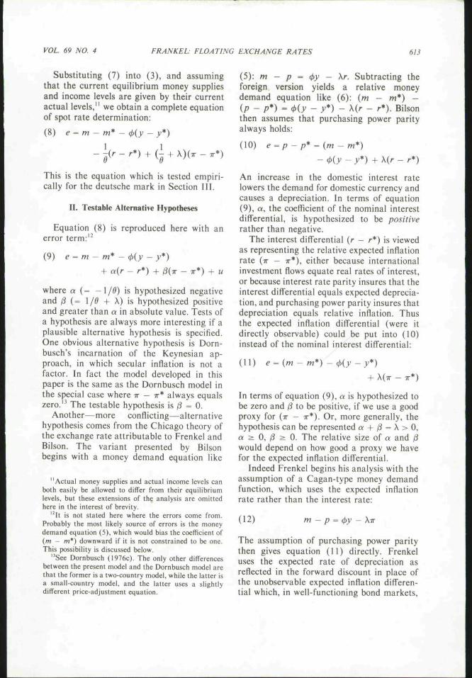
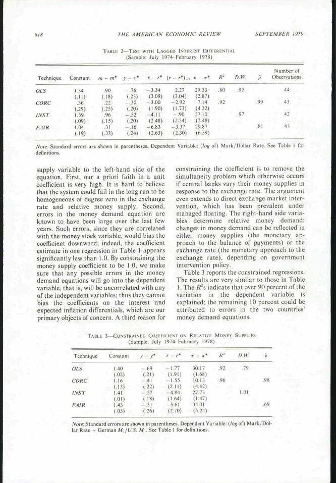
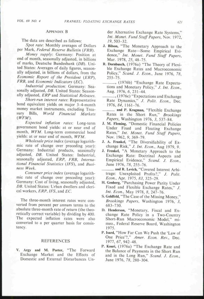
\ f i t t e d\

FIGURE l. Pt.OT OF {log OF) MARK/DOLLAR RATE.

OLS REGRESSION FROM TABLE 1

the (negative) coefficient on the nominalinterest differential and the coefficient on theexpected inflation differential is an estimateof the semielasticity of money demand withrespect to the interest rate; when converted toa per annum basis, the estimate is 6.0, whichprovides another favorable cross-check.'^

The point estimate of a is -5 .4 . Thisimplies that when a disturbance creates adeviation from purchasing power parity,(1 - 1/5.4 =) 81-5 percent of the deviation isexpected to remain after one quarter, and{.^\5'^ =) 44.1 percent is expected to remainafter one year. The estimate of ^ on a perannum basis is {-log .441 =) .819. Previouswork on the speed of adjustment to purchas-ing power parity is less definitive than esti-mates of money demand elasticities, but thepresent estimates of the expected speed ofadjustment appear reasonable."*

"The semielasticity estimate and an average interestrate of around 6 percent imply an interest elasticity ofaround (6,0 x .06 =) .36, which is in the range ofestimates of the long-run elasticity made by StephenGoldfeld and others.

'*Hans Genberg estimates for Germany that 37percent of an initial divergence from purchasing powerparity disappears after one year.

As a final indication of the support Table 1provides for the real interest differentialhypothesis, the Rh are high. Figure 1 shows aplot of the equation's predicted values and theactual exchange rate values. The equationtracks the mark's 1974 appreciation, 1975depreciation, and 1976-77 appreciation."

To apply the estimated equation, let usconvert it to the form:

- 1.39

- 1.35(r- 7.35(7r

where a and /3 have been divided by four foruse with per annum interest rates and thecoefficient on the relative money supply hasbeen set to 1.0. The expression can be decom-posed into the equilibrium exchange rate

e = 1-39 + {m - m*) - .52iy - y*)+ 6.00(7r - IT*)

"The equation fails to track the continued sharpdepreciation of the dollar in January and February of1978. The regressions that were reported in earlierversions of this paper did not include this period, andconsequently appeared more favorable to the real interestdifferential model.


and the size of the overshooting

e -e= - 1 . 3 5 [ ( r - 7r) - (r* - TT*)]

As an illustration, let us conduct the hypo-thetical experiment of an unexpected Ipercent expansion in the U.S. relative moneysupply. If the monetary expansion is consid-ered a once-and-for-all change, then the equi-librium mark/dollar rate decreases by 1.0percent. But in the short run the expansionalso has liquidity effects; the interest semi-elasticity of 6.00 implies a fall in the nominalinterest rate of (1 percent/6.00 =) 17 basispoints.^" This fall in the real interest differen-tial induces an incipient capital outflow whicbin turn causes the currency to depreciatefurther, until it overshoots its new equilibriumby (1.35 X .17 percent =) .23 percent. Thetotal initial depreciation is 1.23 percent.

This calculation assumes no change in theexpected inflation rate. If tbe monetaryexpansion signals a new higher target formonetary growth, then the effect could bemuch greater.'' Suppose the annualized 12percent increase raises the expected inflationrate by, say, 1 percent per annum. Then therewill be an additional depreciation of 6.00percent on account of the lower demand formoney in long-run equilibrium plus 1.35percent more overshooting on account of thefurther reduced real interest differential.Thus the total initial depreciation would be8.58 percent, of whicb 7.00 percent representslong-run equilibrium and 1.58 percent repre-sents short-run overshooting.

After the initial effects, the system movestoward the new equilibrium as described inAppendix A. provided capital is perfectlymobile and future money supplies do notdeviate from their expected values. American

^Here we are assuming (for the first time) that theestimated long-run interest semietasticity holds in theshort run as well. If money demand is subject to laggedadjustment, then the short-run effect of a monetarycontraction on the interest rate and hence on theexchange rate would be greater than that calculated here.However the theory and econometrics behind equation(8) would be completely unaffected.

"On ihe other hand, if some of the expansion isexpected lo be reversed in the following month, then thedecrease in the equilibrium rate would be correspond-ingly smaller.

goods are cheaper than German goods; higherdemand will gradually drive up Americanprices faster than the rate of monetarygrowth, which in turn will drive up U.S.nominal interest rates, reduce the overshoot-ing, and cause the spot rate to rise backtowards its new equilibrium. After a year,approximately 44 percent of the initial realinterest differential and purchasing powerparity deviation will have been closed. In themeantime, there should be an expansionaryeffect on demand for U.S. output; lower realU.S. prices will stimulate net exports andlower real U.S. interest rates will stimulateinvestment. However, any efiTects on outputhave not been modelled in this paper.^^

IV. Econometric Extensions

It is possible that adjustment in capitalmarkets to changes in the interest differentialis not instantaneous, and that lagged interestdifferentials should be included in the regres-sions. Formally, we could argue that due totransactions costs, tbe forward discountadjusts fully to the interest differential with aone-month lag:

(13) d=h{r-r*) -H (1 - h ) { r - r * ) _ ,

When (13) is used in place of (1), the spotrate equation (8) is replaced by

(14) e = {m-m*)

- {h/d){r - r*) - {]

The results of regressions with a lagged inter-est differential are reported in Table 2. Thecoefficient on the lagged interest differentialis insignificantly less than zero. This evidencesupports tbe idea that capital is perfectlymobile.

There are several reasons why one mightwish to constrain the coefficient on the rela-tive money supply to be 1.0 in these regres-sions, in effect moving the relative money

"The assumption of exogenous output can be relaxedby assuming that output is demand determined. Then anecessary condition for overshooting is that the elasticityof demand with respect lo relative prices is less than 1.0.See the Appendix to Dornbusch {1976c).

6/5 THE AMERICAN ECONOMIC REVIEW SEPTEMBER 1979

TABLE 2—TEST WITH LAGGED INTEREST DIFFERENTIAL(Sample: July 1974-February 1978)

Technique Constant m y - y r* {r - r»)_, -IT - TT' D.W.Number of

Observations

OLS

CORC

INST

FAIR

1.34(.11).56

(.29)1.39(.09)1.04(.19)

.90(.18).22

(-25).96

(.15).31

(.33)

- .76(.23)

- .30(.20)

- .52(.20)

- .16(-24)

-3.34(3.09)

-3.00(1.90)

-4.11(2.48)

-6.83(2.63)

2.27(3.04)

-2.92(1.73)- .90(2.54)-3.37(2.30)

29.33(2.87)7.14

(4.32)27.10(2.48)29.87(6.59)

.80

.92

.82

.97

.99

.SI

44

43

43

Note. Standard errors are shown in parentheses. Dependent Variable: (log of) Mark/Dollar Rate, See Table 1 fordefinitions.

supply variable to the left-band side of theequation. First, our a priori faith in a unitcoefficient is very higb. It is hard to believethat the system could fail in the long run to behomogeneous of degree zero in the exchangerate and relative money supply. Second,errors in the money demand equation areknown to have been large over tbe last fewyears. Sucb errors, since tbey are correlatedwith the money stock variable, would bias thecoefficient downward; indeed, the coefficientestimate in one regression in Table I appearssignificantly less than 1.0. By constraining themoney supply coefficient to be 1.0, we makesure that any possible errors in the moneydemand equations will go into the dependentvariable, that is, will be uncorrelated with anyof the independent variables; thus they cannotbias the coefficients on the interest andexpected inflation differentials, which are ourprimary objects of concern. A third reason for

constraining the coefficient is to remove thesimultaneity problem which otherwise occursif central banks vary their money supplies inresponse to the exchange rate. The argumenteven extends to direct exchange market inter-vention, which has been prevalent undermanaged floating. The right-hand side varia-bles determine relative money demand;changes in money demand can be reflected ineither money supplies (the monetary ap-proach to the balance of payments) or theexchange rate (the monetary approach to theexchange rate), depending on governmentintervention policy.

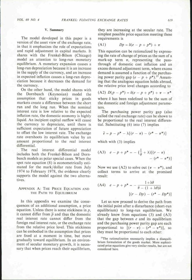
Table 3 reports the constrained regressions.The results are very similar to those in Table1. The /?^s indicate that over 90 percent of thevariation in the dependent variable isexplained; the remaining 10 percent could beattributed to errors in the two countries'money demand equations.

TABLE 3—CONSTRAINED COEFFICIENT ON RELATIVE MONEY SUPPLIES(Sample: July 1974-February 1978)

Technique

OLS

CORC

INST

FAIR

Constant

1.40(.02)1.16(.13)1.41(.01)1.43(.03)

y - y*

- .69(-21)

-.41(.22)

- .52(.18)

- .31(.26)

r - r*

(1.91)-1,55(2.11)

-4.84(1.64)

-5.61(2.70)

IT - T *

30.17(1.68)10.13(4.82)27.73(1.47)34.01(4.24)

R'

.92

,96

D.W.

.79

1.01

P

m

.69

Noie\ Standard errors are shown in parentheses. Dependent Variable: (log of) Mark/Dol-lar Rale H- German M,/U.S. M^. See Table 1 for definitions.

VOL. 69 NO. 4 FRANKEL FLOATING EXCHANGE RATES 619

V. Summary

The model developed in this paper is aversion of the asset view of the exchange rate,in that it emphasizes the role of expectationsand rapid adjustment in capital markets. Itshares with the Frenkel-Bilson (Chicago)model an attention to long-run monetaryequilibrium. A monetary expansion causes along-run depreciation because it is an increasein the supply of the currency, and an increasein expected Inflation causes a long-run depre-ciation because it decreases the demand forthe currency.

On the other hand, the model shares withthe Dornbusch (Keynesian) model theassumption that sticky prices in goodsmarkets create a difference between the shortrun and the long run. When the nominalinterest rate is low relative to the expectedinflation rate, the domestic economy is highlyliquid. An incipient capital outflow will causethe currency to depreciate, until there issufficient expectation of future appreciationto offset the low interest rate. The exchangerate overshoots its equilibrium value by anamount proportional to the real interestdifferential.

The real interest differential modelincludes both the Frenkel-Bilson and Dorn-busch models as polar special cases. When thespot rate equation (8) is econometrically esti-mated for the mark/dollar rate from July1974 to February 1978, the evidence clearlysupports the model against the two alterna-tives.

APPENDIX A: THE PRICE EQUATION ANDTHE PATH TO EQUILIBRIUM

In this appendix we examine the conse-quences of an additional assumption, a priceequation. Unless there is some stickiness in p,it cannot differ from p and thus the domesticreal interest rate cannot differ from theforeign real interest rate, or the exchange ratefrom the relative price level. This stickinesscan be embodied in the assumption that pricesare fixed at a moment in time, but movegradually toward equilibrium. In an environ-ment of secular monetary growth, it is neces-sary that when prices reach their equilibrium.

they are increasing at the secular rate. Thesimplest possible price equation meeting theserequirements is

(Al) Dp = 8(e- p + p*) + 7r

This equation can be rationalized by express-ing the rate of change of prices as the sum of amark-up term x, representing the pass-through of domestic cost inflation and anexcess demand adjustment term, where excessdemand is assumed a function of the purchas-ing power parity gap (e - p + p*) . " Assum-ing that the analogous equation holds abroad,the relative price level changes according to

(A2) D{p - p*) =8{e-p+p*) + w-Tr*

where 5 has been redefined to be the sum ofthe domestic and foreign adjustment parame-ters.

The purchasing power parity gap (alsocalled the real exchange rate) can be shown tobe proportional to the real interest differen-tial. Substituting (6) into (7) implies

e=p-p*-X[(r-w)-ir*-T*)]

which with (3) implies

(A3)

Now we use (A2) to solve out (7r - TT*), andcollect terms to arrive at the promisedresult:

i+\e(A4) e - p + p* = -

[(r-Dp) -(r* -Dp*)]

Let us now proceed to derive the path fromthe initial point after a disturbance (short-runequilibrium) to long-run equilibrium. Wealready know from equations (3) and (A3)that the gap between e and its equilibriumand the purchasing power parity gap are eachproportional to [(r - x) - (r* — 7r*)], sothey must be proportional to each other;

"The rationalization necessarily implies a disequili-brium formulation of the goods market. More sophisti-cated price equations give very similar results, but are notconsidered here.


(A5) {e - p + p*) = {\ + \d){e - e)

Using e - p + p* = 0 and (A5).

(A6) e - p -\- p* = {e -e)

- ip -p) + (p* -

I + \d

\6Up - P*) - iP - P*)]

Substituting (A6) into (A2),

(A7) Dip - p*) = -'d(\+K6)/Xd

[ip-p*) -ip-p*)] + X - X *

This differential equation has the solution

(A8) ip- p*), = ip-p*\

-hexp[-5(l + \d/Xd)t][{p - p*),

-ip-p*U

The relative price level moves toward itsequilibrium at a speed which is proportionalto the gap. The equilibrium relative pricelevel, it must be remembered, is itself increas-ing at the rate ir — ir*.

An analogous equation holds for e. Equa-tions (A5) and (A6) tell us

{A9) e^e= -^Up-p*) - {p - p*)]Af

Taking the time derivative,

(AlO) De^ -:~D[ip- p*)

-ip-p*)] + Oe

5(1 + \9)

^ ~ X̂

• {e -e) + TT - T*

This differential equation has the solution

(All) e, = e,\e)/X6)l]{e - e)^

Comparing (AlO). the expression for therate of change of the spot rate if there are nofurther disturbances, with (2), the expressionfor the expected rate of change of theexchange rate, we see that the two are of thesame form. Perfect foresight (or rationalexpectations in the stochastic case) holds if d= 6(1 + \0)/\6, which has the solution

{A12)2X

1/2

2X

Here we throw out the negative root because 8was assumed positive when (2) was specified.We can see that 6^ increases with 8, the speedof adjustment in goods markets. In turn, weknow from equation (3) that the sensitivity ofthe exchange rate to monetary changesdecreases with 6. The implication is that theslower is adjustment in the goods market, themore volatile must the exchange rate be inorder to compensate.

It is easy to show that we could havederived (2) from the rest of the model and theassumptions of perfect foresight and stability,instead of assuming the form of expectationsdirectly. Substituting the relative moneydemand equation (6) into the interest paritycondition (I),

(A13) d^{[/X)[(p-p*)-im-m*)

The perfect foresight assumption is d = De.Equation (AI3) and the price equation (A2)can be represented in matrix form:

0 l / \De

D{p-p*)

IT — TT^

Let -0, and -6-, be the characteristic roots:

1/X

= -de + e' -

The solution is given by (A 12). The path of eis given by

{e - = a,

The system is stable if and only if O; = 0,which, with the initial condition a, ={e - e)o, implies equation (2), and thepositive root from (A 12).

VOL. 69 NO. 4 FRANKEL FLOATING EXCHANGE RATES 621

APPENDIX B

The data are described as follows:Spot rate: Monthly averages of Dollars

per Mark, Eederal Reserve Bulletin (ERB).Money supply: Germany: Position at

end of month, seasonally adjusted, in billionsof marks, Deutsche Bundesbank (DB). Uni-ted States: Averages of daily figures, season-ally adjusted, in billions of dollars, from theEconomic Report of the President (ERP),ERB, and Economic Indicators {EC).

Industrial production: Germany: Sea-sonally adjusted, DB. United States: Season-ally adjusted, ERP and Statistical Releases.

Short-run interest rates: Representativebond equivalent yields on major 3-4-monthmoney market instruments, excluding Trea-sury Bills, World Einancial Markets{WEM).

Expected inflation rates: Long-termgovernment bond yields: at or near end ofmonth, WEM. Long-term commercial bondyields: at or near end of month, WEM.

Wholesale price index (average logarith-mic rate of change over preceding year):Germany: Industrial products, seasonallyadjusted, DB. United States: Industrial,seasonally adjusted, ERP, ERB, Interna-tional Einancial Statistics (lES), and Busi-ness Week.

Consumer price index (average logarith-mic rate of change over preceding year):Germany: Cost of living, seasonally adjusted.DB. United States: Urban dwellers and cleri-cal workers, ERP, lES, and EC

The three-month interest rates were con-verted from percent per annum terms to theabsolute three-month rate of return (the theo-retically correct variable) by dividing by 400.The expected inflation rates were alsoconverted to a per quarter basis for consis-tency.

REFERENCES

V. Argy and M. Porter, "The ForwardExchange Market and the Effects ofDomestic and External Disturbances Un-

der Alternative Exchange Rate Systems,"Int. Monet. Eund Staff Papers, Nov. 1972,79,503-32.

J. Bilson, "The Monetary Approach to theExchange Rate—Some Empirical Evi-dence," Int. Monet. Eund Staff Papers,Mar. 1978, 25, 48-75.

R. Dornbusch, (1976a) "The Theory of Flexi-ble Exchange Rates and MacroeconomicPolicy," Scand. J. Econ., June 1976, 78,255-75.

., (1976b) "Exchange Rate Expecta-tions and Monetary Policy," J. Int. Econ,Aug. 1976,(5, 231-44.

-, (1976c) "Expectations and ExchangeRate Dynamics," J. Polit. Econ., Dec.1976,8-^, 1161-76.

and P. Krugman, "Flexible ExchangeRates in the Short Run," BrookingsPapers, Washington 1976, i , 537-84.

J. M. Fleming, "Domestic Financial PoliciesUnder Fixed and Floating ExchangeRates," Int. Monet. Eund Staff Papers,Nov. 1962, 9, 369-79.

J. A. Frankel. "The Diversifiability of Ex-change Risk," J. Int. Econ., Aug 1979, 9.

J. Frenkel, "A Monetary Approach to theExchange Rate: Doctrinal Aspects andEmpirical Evidence," Scand. J. Econ.,June 1976, 78, 255-76.

and R. Levich, "Covered Interest Arbi-trage: Unexploited Profits?," J. Polit.Econ., Apr. 1975, 83, 325-29.

H. Genberg, "Purchasing Power Parity UnderFixed and Flexible Exchange Rates," J.Int. Econ., May 1978, 8, 247-76.

S. Goldfeld, "The Case of the Missing Money,"Brookings Papers, Washington 1976, 3,683-730.

D. Henderson, "Monetary, Fiscal and Ex-change Rate Policy in a Two-CountryShort-Run Macroeconomic Model," mi-mec. Federal Reserve Board, Washington1975.

P. hard, "How Far Can We Push the 'Law ofOne Price'?," Amer. Econ. Rev., Dec.1977,67,942^8.

P. Kouri, (1976a) "The Exchange Rate andthe Balance of Payments in the Short Runand in the Long Run," Scand. J. Econ.,June 1976, 78, 280-304.


, (1976b) "Foreign Exchange MarketSpeculation and Stabilization Policy UnderFlexible Exchange Rates," paper presentedat Conference on the Political Economy ofInflation and Unemployment in OpenEconomies, Athens, Oct. 1976.

I. Kravis and R. Lipsey, "Export Prices and theTransmission of Inflation," Amer. Econ.Rev. Proc, Feb. 1977, 67, 155-63.

Robert Mundell, "Exchange Rate Margins andEconomic Policy," in J. Carter Murphy,ed.. Money in the International Order,Dallas 1964.

, International Economics, New York1968.

M. Mtissa, "The Exchange Rate, the Balanceof Payments and Monetary and FiscalPolicy Under a Regime of ControlledFloating," Scand. J. Econ., June 1976, 78,229^8 .

, "Real and Monetary Factors in aDynamic Theory of Foreign Exchange,"mimeo., Univ. Chicago, Apr. 1977.

J. Niehans, "Some Doubts About the Efficacyof Monetary Policy Under Flexible Ex-

change Rates," / . Int. Econ., Aug. 1975, 5,275-81.

M. V. N. Whitman, "Global Monetarism andthe Monetary Approach to the Balance ofPayments," Brookings Papers, Washing-ton 1975, i , 491-556.

Board of Governors of the Federal Reserve System,Statistical Releases, Washington, variousissues.

, Fed. Res. Bull., Washington, variousissues.

Business Week, various issues.Deutsche Bundeshank, Statistical Supplements

to Monthly Reports, Bonn, various issues.International Monetary Fund, International Fi-

nancial Statistics, Washington, variousissues.

Morgan Guaranty and Trust Co., World Finan-cial Markets, New York, various issues.

U.S. Congress, Joint Economy Committee,Economic Indicators, Washington, variousissues.

U.S. Council of Economic Advisors, EconomicReport of the President, Washington, vari-ous issues.

on the mark: a theory of floating exchange rates based … · rates based on real interest...

Documents