on the origin of utility, weighting, and discounting

Submitted to Econometrica

On the Origin of Utility, Weighting,and Discounting Functions: How

They Get Their Shapes and How toChange Their Shapes

Neil Stewart, Stian Reimers and Adam J. L. Harris

October 14, 2011

Submitted to Econometrica

1 1

2 2

3 3

4 4

5 5

6 6

7 7

8 8

9 9

10 10

11 11

12 12

13 13

14 14

15 15

16 16

17 17

18 18

19 19

20 20

21 21

22 22

23 23

24 24

25 25

26 26

27 27

28 28

29 29

ON THE ORIGIN OF UTILITY, WEIGHTING, AND DISCOUNTING

FUNCTIONS: HOW THEY GET THEIR SHAPES AND HOW TO CHANGE THEIR

SHAPES1 2

NEIL STEWARTa , STIAN REIMERSb AND ADAM J. L. HARRISc

We present a theoretical account of the shapes of utility, probability weighting, and

temporal discounting functions. In an experimental test of the theory, we systematically

change the shape of revealed utility, weighting, and discounting functions by manipu-

lating the distribution of monies, probabilities, and delays in the questions used to elicit

them. The data demonstrate that there is no stable mapping between attribute values and

their subjective equivalents. This is a profound challenge to expected and discounted

utility theories, and also their descendants such as prospect theory and hyperbolic dis-

counting theory. These theories simply assert a particular shape for the stable mapping

in order to describe choice data. We explain where the shapes comes from and, in de-

scribing the mechanism by which people choose, explain why the shape depends on the

distribution of gains, losses, risks, and delays in the environment.

KEYWORDS: revealed utility, cardinal utility, ordinal utility, probability weighting,

subjective probability, temporal discounting, delay discounting, stable preferences, de-

cision by sampling, range frequency theory, risky choice, decision under risk, intertem-

poral choice, decision under delay.

1We thank James Adelman for valuable help with the logistic regression analysis and Gor-

don D. A. Brown, Tatiana Kornienko, Graham Loomes, Will Matthews, Dani Navarro-Martinez,

Ganna Pogrebna, and Christoph Ungemach for insightful discussion. This research was sup-

ported by ESRC grants RES-062-23-0952 and RES-000-22-3339.2Raw data and the R source code for all analyses are available from the first author.aDepartment of Psychology, University of Warwick, Coventry, CV4 7AL, UK.

[email protected]; http://www.stewart.warwick.ac.ukbDepartment of Psychology, City University, Northampton Square, London, EC1V 0HB, UK.

[email protected] of Cognitive, Perceptual and Brain Sciences, University College London, 26

Bedford Way, London, WC1H 0AP, UK. [email protected]

1ectaart.cls ver. 2006/04/11 file: revealed_functions.tex date: October 14, 2011

http://www.econometricsociety.org/

mailto:[email protected]

http://www.stewart.warwick.ac.uk



2

1 1

2 2

3 3

4 4

5 5

6 6

7 7

8 8

9 9

10 10

11 11

12 12

13 13

14 14

15 15

16 16

17 17

18 18

19 19

20 20

21 21

22 22

23 23

24 24

25 25

26 26

27 27

28 28

29 29

1. INTRODUCTION

Central to our economic behavior are the attributes money, probability, and

time. Our representations of these attributes, and our integration of information

across these attributes, is thought to determine our economic behavior. The theo-

ries of decision under risk and delay generally assume that we transform money,

probability, and delay into subjective equivalents, and then integrate informa-

tion across these equivalents. These transformations are typically modeled using

utility (or value), weighting, and discounting functions. In this paper we present

a theory of this process which accounts for the previously observed nature of

these functions. A prediction of this theory is that these transformations are not

stable, and four experimental tests confirm this prediction. We show that by ma-

nipulating the distribution of monies, probabilities, and delays in the question

set used to elicit utility, weighting, and discounting functions we can systemat-

ically change their shape. That is, we show that if you ask different questions

the revealed subjective values of given monies, probabilities, and delays can be

adjusted, to some extent, at the experimenter’s will. We argue that, although it is

possible to derive utility functions, subjective probability functions, and tempo-

ral discounting functions from behavioral data (such as a series of choices), these

psychoeconomic functions have no psychological reality: There are no look up

tables that convert from real-world attributes to their subjective equivalents in

people’s heads. We also argue that, at the individual level, these functions have

no economic use: The functions do not provide a parsimonious description of

people’s choices, because the functions vary with changes to the context that

should be trivial.

Below we review the measurement and use of psychoeconomic functions first

in decision under risk (Section 2) and then in decision under delay (Section 3).

We illustrate how the psychoeconomic functions are shaped to describe the choices

that people make. We then review evidence that suggests that the psychoeco-

nomic functions may be influenced by the distribution of attribute values (Sec-

ectaart.cls ver. 2006/04/11 file: revealed_functions.tex date: October 14, 2011

3

1 1

2 2

3 3

4 4

5 5

6 6

7 7

8 8

9 9

10 10

11 11

12 12

13 13

14 14

15 15

16 16

17 17

18 18

19 19

20 20

21 21

22 22

23 23

24 24

25 25

26 26

27 27

28 28

29 29

tion 4). We present a theoretical account of utility, weighting, and discounting

functions that explains both why these functions take the shapes they do and also

explains how these shapes are influenced by the distribution of attribute values

(Section 5). We present an experimental test of the theory (Section 6). Finally,

we close with discussion and implications (Section 7).

2. DECISION UNDER RISK

Expected utility is the normative model for risky decision making (von Neu-

mann and Morgenstern, 1947). In expected utility theory, incremental wealth has

diminishing marginal utility—the utility of my second $100, for example, is just

a little bit lower than the utility of my first $100. To capture this, wealth is trans-

lated into utility by a concave function, initially quite steep but then later more

flat showing a high sensitivity to initial increases in wealth but then a lower sensi-

tivity to later increases. To choose between risky options, the average or expected

utility of each available course of action is calculated and the action maximizing

expected utility is selected.

Economists and psychologists have created a large set of models of decision

under risk that follow the expected utility framework. Each model adapts utility

theory to incorporate some psychological insight based, often, on observations of

people’s choice behavior. Prospect theory (Kahneman and Tversky, 1979; Tver-

sky and Kahneman, 1992) is perhaps the most famous, but there are many other

significant theories (e.g., Birnbaum, 2008; Birnbaum and Chavez, 1997; Buse-

meyer and Townsend, 1993; Edwards, 1962; Loomes and Sugden, 1982; Quig-

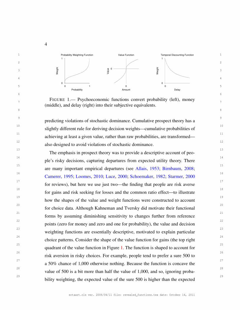
gin, 1993; Savage, 1954). In prospect theory terminology, a value function con-

verts money into value (the analogue of utility) and a weighting function converts

probability into a decision weight. Figure 1 gives example value and weighting

functions.

In fact, prospect theory departs slightly from this description. Original prospect

theory has an initial series of editing rules designed to prevent the model from


4

1 1

2 2

3 3

4 4

5 5

6 6

7 7

8 8

9 9

10 10

11 11

12 12

13 13

14 14

15 15

16 16

17 17

18 18

19 19

20 20

21 21

22 22

23 23

24 24

25 25

26 26

27 27

28 28

29 29

0

1

0 1

Weig

ht

Probability

Probability Weighting Function

0

0

Valu

e

Amount

Value Function

0

1

0

Weig

ht

Delay

Temporal Discounting Function

FIGURE 1.— Psychoeconomic functions convert probability (left), money(middle), and delay (right) into their subjective equivalents.

predicting violations of stochastic dominance. Cumulative prospect theory has a

slightly different rule for deriving decision weights—cumulative probabilities of

achieving at least a given value, rather than raw probabilities, are transformed—

also designed to avoid violations of stochastic dominance.

The emphasis in prospect theory was to provide a descriptive account of peo-

ple’s risky decisions, capturing departures from expected utility theory. There

are many important empirical departures (see Allais, 1953; Birnbaum, 2008;

Camerer, 1995; Loomes, 2010; Luce, 2000; Schoemaker, 1982; Starmer, 2000

for reviews), but here we use just two—the finding that people are risk averse

for gains and risk seeking for losses and the common ratio effect—to illustrate

how the shapes of the value and weight functions were constructed to account

for choice data. Although Kahneman and Tversky did motivate their functional

forms by assuming diminishing sensitivity to changes further from reference

points (zero for money and zero and one for probability), the value and decision

weighting functions are essentially descriptive, motivated to explain particular

choice patterns. Consider the shape of the value function for gains (the top right

quadrant of the value function in Figure 1. The function is shaped to account for

risk aversion in risky choices. For example, people tend to prefer a sure 500 to

a 50% chance of 1,000 otherwise nothing. Because the function is concave the

value of 500 is a bit more than half the value of 1,000, and so, ignoring proba-

bility weighting, the expected value of the sure 500 is higher than the expected


5

1 1

2 2

3 3

4 4

5 5

6 6

7 7

8 8

9 9

10 10

11 11

12 12

13 13

14 14

15 15

16 16

17 17

18 18

19 19

20 20

21 21

22 22

23 23

24 24

25 25

26 26

27 27

28 28

29 29

value of the 50% chance of 1,000 otherwise nothing. That is, the value function

is concave for gains to describe risk aversion. We don’t consider losses in this

paper, but note here for completeness that the value function is convex for losses

because, for moderate probabilities, people tend to be risk seeking for gambles

involving losses, rather than risk averse as they are for gambles involving gains

(see Tversky and Kahneman, 1992 for a description).

The shape of the weighting function is also constructed to describe the choices

that people make. Consider, for example, the common ratio effect (Allais, 1953).

In a choice between 3,000 for sure and an 80% chance of 4,000 otherwise noth-

ing, people are risk averse, as above, and prefer the 3,000 for sure. However, in

a choice between a 25% chance of 3,000 otherwise nothing and a 20% chance

of 4,000 otherwise nothing, people prefer the 20% chance of 4,000 otherwise

nothing. Because the second choice is derived from the first by multiplying prob-

abilities by 1/4, participants should prefer the more risky option in both cases or

the less risky option in both cases. Thus the empirical finding is not consistent

with expected utility theory. Kahneman and Tversky account for these data by

assuming that people are most sensitive to changes in small or large probabilities

and are least sensitive to changes in intermediate probabilities. Thus the decision

weights of 20% and 25% are quite similar but the weights of 80% and 100% are

quite different. That is, the weighting function takes its inverse-S shape in order

to describe the common ratio effect (and other choice patterns) that people make.

3. DECISION UNDER DELAY

The normative starting point for intertemporal choices is discounted utility

theory (Samuelson, 1937). When choosing between a series of delayed out-

comes, each outcome is discounted by reducing its value by a constant fraction

for every unit of time it is delayed. The value of a delayed outcome thus dimin-

ishes exponentially with the length of the delay, and this leads to preferences that

remain consistent over time.


6

1 1

2 2

3 3

4 4

5 5

6 6

7 7

8 8

9 9

10 10

11 11

12 12

13 13

14 14

15 15

16 16

17 17

18 18

19 19

20 20

21 21

22 22

23 23

24 24

25 25

26 26

27 27

28 28

29 29

As with decision under risk, psychologists and economists have modified this

discounted utility framework to incorporate psychological insight based on ob-

servation. Perhaps the most significant model is hyperbolic discounting (Ainslie,

1975; Loewenstein and Prelec, 1992, but see also Laibson, 1997; Read, 2001;

Scholten and Read, 2010). Here we select one example behavioral finding to il-

lustrate the descriptive model, but there are many (see Loewenstein and Prelec,

1992; Scholten and Read, 2010 for reviews). In the common difference effect

people have a tendency to reverse their preferences when a common interval is

added or subtracted from the delays of each option. For example, in a choice

between 100 in 10 days and 110 in 11 days, people might prefer the later larger

reward of 110 in 11 days. However, when the same rewards are brought forwards

9 days, so people are choosing between 100 in 1 day and 110 in 2 days, peo-

ple might prefer the smaller sooner reward. That is, there is more discounting in

moving from 1 to 2 days than from 10 to 11 days (Thaler, 1981). To explain find-

ings like this, Loewenstein and Prelec (1992, see also Mazur, 1987) suggested

that discounting was hyperbolic, not exponential (see Figure 1). One property of

a hyperbolic function is that the discount rate is initially high and then decreases.

Thus large discounting from 1 to 2 days makes the smaller sooner option rel-

atively more attractive but the reduced discounting from 10 to 11 days makes

the later larger option relatively more attractive. Note that the motivation for the

choice of discounting function is the same as the motivations for the choice of

utility and weighting functions: the goal is to describe the choices that people

make.

4. MALLEABILITY OF RISKY AND DELAYED CHOICES

Below we review a series of studies that demonstrate that choices and valua-

tions of risky and delayed choices are affected by the distributions of amounts,

probabilities, and delays recently experienced. These findings are not consistent

with expected utility, discounted utility, or their derivatives. To foreshadow the


7

1 1

2 2

3 3

4 4

5 5

6 6

7 7

8 8

9 9

10 10

11 11

12 12

13 13

14 14

15 15

16 16

17 17

18 18

19 19

20 20

21 21

22 22

23 23

24 24

25 25

26 26

27 27

28 28

29 29

later theory section, in all of these studies, people behave as if the subjective

value of an amount, risk, or delay is given by its rank position in the context

created by other recently experienced amounts, risks, and delays. The first set of

studies describes how previously encountered amounts, risks, and delays affect

current choices. The second set of studies describes how the distribution of po-

tential values affects valuation. The final set describes how choices are affected

by the set of alternatives on offer.

In decision under risk, Stewart (2009) demonstrated that a target choice be-

tween a 30% chance of 100 points and a 40% chance of 75 points can be reversed

by manipulating the distributions of probabilities and amounts encountered just

before the choice. When previous choices contained amounts 25, 50, 75, 100,

125, and 150 points and probabilities 30%, 32%, 34%, 36%, 38%, and 40%,

people preferred a 40% chance of 75 points. In making this choice, people are

behaving as if the difference in amounts is relatively small (the ranks of 75 and

100 points are very similar, ranking 4th and 3rd respectively) but the difference

in probabilities is relatively large (the ranks of 30% and 40% are very different,

ranking 6th and 1st respectively). If people feel that 40% is much better than

30% but that 100 points is only slightly better than 75 points, a 40% chance of

75 points will be more attractive than a 30% chance of 100 points. In contrast,

when previous choices contained amounts 75, 80, 85, 90, 95, and 100 points

and probabilities 10%, 20%, 30%, 40%, 50%, and 60%, people preferred a 30%

chance of 100 points. In this new context, the ranks of 30% and 40% are very

similar but the ranks of 75 and 100 points are very different.

Extending this design, Ungemach, Stewart, and Reimers (2011) have exam-

ined how the distribution of attribute values we experience every day affects

choices. In one study, Ungemach et al. found that customers leaving a super-

market evaluated the prizes on offer in two simple lotteries against the cost of

purchases made a few minutes earlier inside a supermarket. One lottery offered

£1.50 with a low probability and the other offered £0.50 with a high probability.


8

1 1

2 2

3 3

4 4

5 5

6 6

7 7

8 8

9 9

10 10

11 11

12 12

13 13

14 14

15 15

16 16

17 17

18 18

19 19

20 20

21 21

22 22

23 23

24 24

25 25

26 26

27 27

28 28

29 29

If most purchases were for amounts between £0.50 and £1.50, people behaved as

if the difference between £0.50 and £1.50 was larger, and selected the £1.50 lot-

tery. Alternatively, if most purchases were for less than £0.50 or more than £1.50,

people behaved as if the difference between £0.50 and £1.50 was smaller, and se-

lected the £0.50 lottery which has the higher probability of winning. Ungemach,

Stewart, and Reimers present similar findings for probability when people gener-

ate a probability for a weather event before making a risky choice and for delay

when people plan for their birthday before making an intertemporal choice. In

both this study and the previous study, the previously encountered attribute val-

ues were irrelevant to the later choice, but differences in the distributions of the

previously encountered attribute values were sufficient to reverse preferences.

The distribution of prices also affects valuations. Birnbaum (1992) and Stew-

art, Chater, Stott, and Reimers (2003) found that, when valuing a risky gamble,

people were influenced by the range and skew of the options available as po-

tential valuations. For example, Birnbaum found that the valuation of a target

gamble was higher when people were offered a negatively skewed set of can-

didate valuations, with more high amounts, than when people were offered a

positively skewed set, with more low amounts. Using an incentive compatible

auction (Becker, DeGroot, and Marschak, 1964), Ariely, Koszegi, Mazar, and

Shampan’er (2008) found that the distribution of prices from which a sale price

was to be randomly drawn affected the reserve price stated by participants in ex-

actly the same way. With negatively skewed sale prices (i.e., more larger prices),

stated reserve prices were higher than with positively skewed sale prices (i.e.,

more smaller prices). In both experiments, a given candidate value or sale price

appears larger in the positive-skew condition because there are many smaller

prices and few larger ones. In contrast, a given value or sale price appears smaller

in the negative-skew condition because there are few smaller prices and many

larger ones. Thus, to match the subjective value of target gamble or auctioned

good, the candidate value or sale price needs to be larger in the negative skew


9

1 1

2 2

3 3

4 4

5 5

6 6

7 7

8 8

9 9

10 10

11 11

12 12

13 13

14 14

15 15

16 16

17 17

18 18

19 19

20 20

21 21

22 22

23 23

24 24

25 25

26 26

27 27

28 28

29 29

condition than in the positive skew condition.

In making a single choice, the available options also affect the level of risk

demonstrated in that choice. Benartzi and Thaler (2001) examined a natural ex-

periment. Employees were asked to allocate their pension funds between bonds

(relatively safe) and stocks (relatively risky). Although all employees were of-

fered at least one stock option and at least one bond option, and thus all em-

ployees could exhibit whatever level of risk they preferred, employees made,

on average, more risky investments if there were more stock options available.

Stewart, Chater, Stott, and Reimers (2003) examine a laboratory analogue, where

people are offered either five risky options or five safe options. Participants in the

different conditions behaved as though they had different levels of risk aversion,

even though participants were randomly assigned to different groups. It is as if

the riskiness of an option is a function of its rank position within the context

against which it is evaluated.

5. A THEORETICAL ACCOUNT

To summarize the above studies, people behave as if the subjective value of

an amount (or probability or delay) is determined, at least in part, by its rank

position in the set of values currently in a person’s head. So, for example, $10

has a higher subjective value in the set $2, $5, $8, and $15 because it ranks 2nd,

but has a lower subjective value in the set $2, $15, $19, and $25 because it ranks

4th.

This suggestion—that subjective value is rank within a sample—is consis-

tent with Parducci’s (1965; 1995) range-frequency model of magnitudes. In this

model, the subjective value of a magnitude is, in part, given by its rank position.

This descriptive model began as an account of scaling of psychophysical quan-

tities, but has more recently been applied in economic contexts such as wage

satisfaction (Boyce, 2009; Brown, Gardner, Oswald, and Qian, 2008).

Stewart, Chater, and Brown (2006, see also Stewart, 2009) proposed the decision-


10

1 1

2 2

3 3

4 4

5 5

6 6

7 7

8 8

9 9

10 10

11 11

12 12

13 13

14 14

15 15

16 16

17 17

18 18

19 19

20 20

21 21

22 22

23 23

24 24

25 25

26 26

27 27

28 28

29 29

by-sampling model of decision making in which the subjective value of an at-

tribute, whether money, probability, or delay, is its rank position in a sample of

attributes (the model is motivated by evidence from psychophysical studies of the

representation of magnitudes). In decision by sampling, rank emerges from the

application of three simple cognitive tools: sampling, binary comparison, and

frequency accumulation. Continuing the above example, $10 is compared to a

sample of other amounts in memory: $2, $5, $8, and $15. In binary comparisons,

$10 looks good compared to $2, $5, $8, but looks bad compared to $15. By accu-

mulating the number of favorable comparisons across the sample, $10 is valued

at 3/4, because three of the four comparisons are favorable. Stewart, Chater, and

Brown (2006) show how these assumptions are sufficient to derive psychoeco-

nomic functions like those in prospect and hyperbolic discounting theories. The

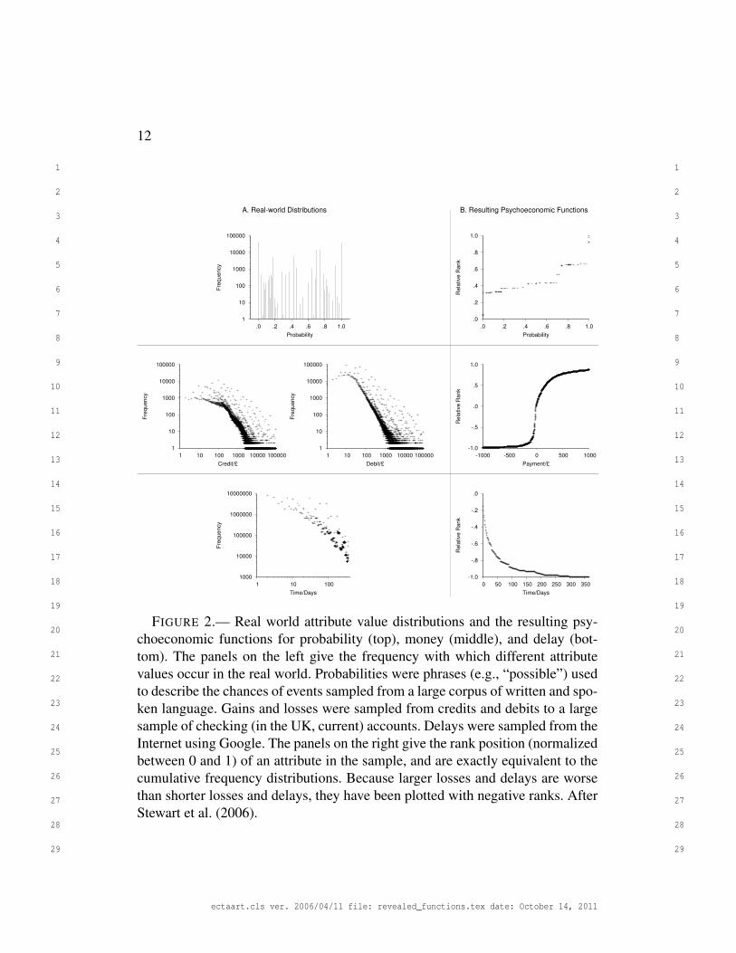
left column of Figure 2 shows the distributions of gains, losses, risks, and delays

in the real world. The right column gives the resulting utility, weighting, and dis-

counting functions under the assumption that monies, risks, and delays are val-

ued by accumulating the number of favorable comparisons against samples from

these real world distributions. For example, because there are more small gains

in the world than large gains, the utility function is concave for gains: Against the

distribution of gains, a £100 increase in a prize from £100 and £200 improves the

rank position substantially more than a £100 increase from £900 to £1,000. No-

tice the resemblance between these functions and the descriptive functions from

prospect and hyperbolic discounting theories in Figure 1. In independent work,

Kornienko (2011) shows formally how these tools provide a cognitive basis for

cardinal utility. Stewart and Simpson (2008) provide details of a decision-by-

sampling process model of Kahneman and Tversky’s (1979) data. An on-line de-

cision by sampling calculator, which gives exact choice probabilities for any set

of prospects, is available at http://www.stewart.warwick.ac.uk/software/DbS/.

Equation 5.1 formalises the expression for the subjective value of an attribute,

although this is scarcely necessary for such a simple theory. The subjective value


11

1 1

2 2

3 3

4 4

5 5

6 6

7 7

8 8

9 9

10 10

11 11

12 12

13 13

14 14

15 15

16 16

17 17

18 18

19 19

20 20

21 21

22 22

23 23

24 24

25 25

26 26

27 27

28 28

29 29

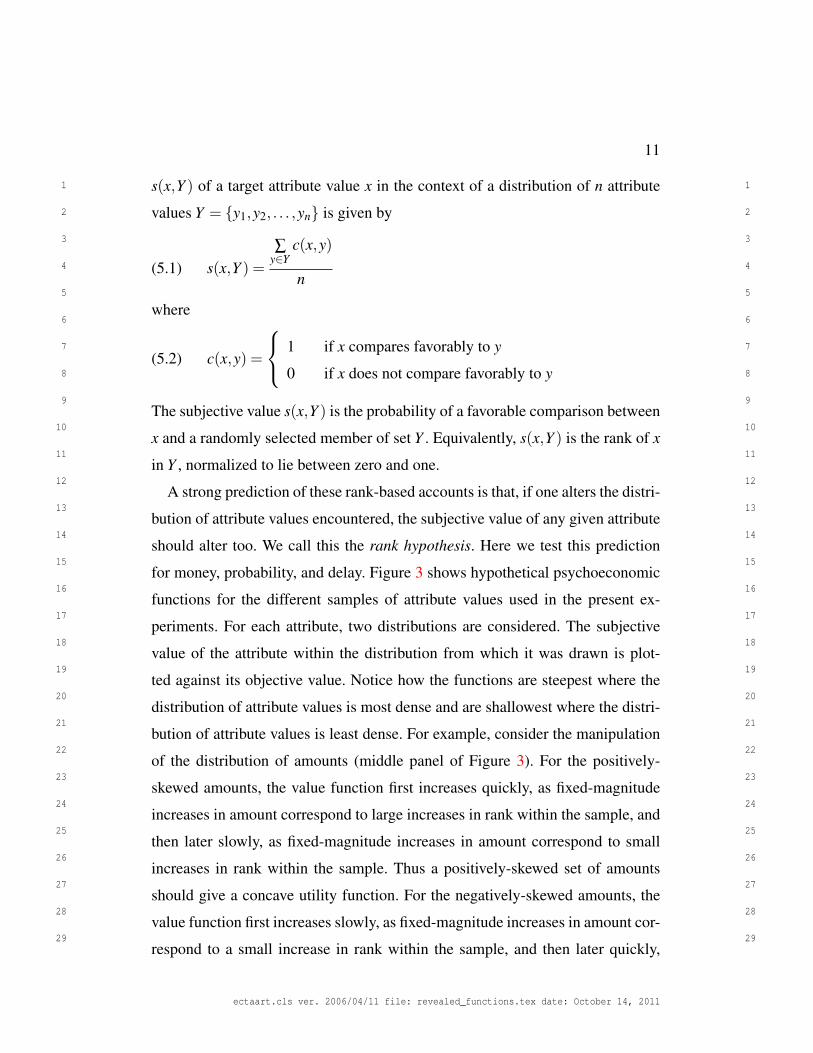
s(x,Y ) of a target attribute value x in the context of a distribution of n attribute

values Y = {y1,y2, . . . ,yn} is given by

(5.1) s(x,Y ) =∑

y∈Yc(x,y)

n

where

(5.2) c(x,y) =

1 if x compares favorably to y

0 if x does not compare favorably to y

The subjective value s(x,Y ) is the probability of a favorable comparison between

x and a randomly selected member of set Y . Equivalently, s(x,Y ) is the rank of x

in Y , normalized to lie between zero and one.

A strong prediction of these rank-based accounts is that, if one alters the distri-

bution of attribute values encountered, the subjective value of any given attribute

should alter too. We call this the rank hypothesis. Here we test this prediction

for money, probability, and delay. Figure 3 shows hypothetical psychoeconomic

functions for the different samples of attribute values used in the present ex-

periments. For each attribute, two distributions are considered. The subjective

value of the attribute within the distribution from which it was drawn is plot-

ted against its objective value. Notice how the functions are steepest where the

distribution of attribute values is most dense and are shallowest where the distri-

bution of attribute values is least dense. For example, consider the manipulation

of the distribution of amounts (middle panel of Figure 3). For the positively-

skewed amounts, the value function first increases quickly, as fixed-magnitude

increases in amount correspond to large increases in rank within the sample, and

then later slowly, as fixed-magnitude increases in amount correspond to small

increases in rank within the sample. Thus a positively-skewed set of amounts

should give a concave utility function. For the negatively-skewed amounts, the

value function first increases slowly, as fixed-magnitude increases in amount cor-

respond to a small increase in rank within the sample, and then later quickly,


12

1 1

2 2

3 3

4 4

5 5

6 6

7 7

8 8

9 9

10 10

11 11

12 12

13 13

14 14

15 15

16 16

17 17

18 18

19 19

20 20

21 21

22 22

23 23

24 24

25 25

26 26

27 27

28 28

29 29

1

10

100

1000

10000

100000

1 10 100 1000 10000 100000

Fre

quency

Credit/£

A. Real-world Distributions B. Resulting Psychoeconomic Functions

1

10

100

1000

10000

100000

1 10 100 1000 10000 100000

Fre

quency

Debit/£

-1.0

-.5

.0

.5

1.0

-1000 -500 0 500 1000R

ela

tive R

ank

Payment/£

1

10

100

1000

10000

100000

.0 .2 .4 .6 .8 1.0

Fre

quency

Probability

.0

.2

.4

.6

.8

1.0

.0 .2 .4 .6 .8 1.0

Rela

tive R

ank

Probability

1000

10000

100000

1000000

10000000

1 10 100

Fre

quency

Time/Days

-1.0

-.8

-.6

-.4

-.2

.0

0 50 100 150 200 250 300 350

Rela

tive R

ank

Time/Days

FIGURE 2.— Real world attribute value distributions and the resulting psy-choeconomic functions for probability (top), money (middle), and delay (bot-tom). The panels on the left give the frequency with which different attributevalues occur in the real world. Probabilities were phrases (e.g., “possible”) usedto describe the chances of events sampled from a large corpus of written and spo-ken language. Gains and losses were sampled from credits and debits to a largesample of checking (in the UK, current) accounts. Delays were sampled from theInternet using Google. The panels on the right give the rank position (normalizedbetween 0 and 1) of an attribute in the sample, and are exactly equivalent to thecumulative frequency distributions. Because larger losses and delays are worsethan shorter losses and delays, they have been plotted with negative ranks. AfterStewart et al. (2006).


13

1 1

2 2

3 3

4 4

5 5

6 6

7 7

8 8

9 9

10 10

11 11

12 12

13 13

14 14

15 15

16 16

17 17

18 18

19 19

20 20

21 21

22 22

23 23

24 24

25 25

26 26

27 27

28 28

29 29

0

1

0 20 40 60 80 100

Weig

ht

Probability/%

Positive

Negative

Probability

0

1

0 100 200 300 400 500

Valu

e

Amount

Positive

Negative

Amount

0

1

0 60 120 180 240 300 360

Weig

ht

Delay

Positive

Uniform

Delay

FIGURE 3.— Hypothetical psychoeconomic functions for probability (left),money (middle), and delay (right). The subjective value of an attribute is itsrank within the distribution of other attribute values (shown above each plot),normalized to lie between 0 and 1.

a fixed-magnitude increases in amount correspond to larger increases in rank

within the sample. Thus a negatively-skewed set of amounts should give a con-

vex utility function. Experiments 1 and 2 explore risky decisions, and investigate

how changing the distribution of amounts and probabilities used to build a set

of choices changes the psychoeconomic functions revealed from those choices.

Experiments 3 and 4 repeat this exercise for intertemporal choices. Experimental

payments were incentive compatible and there was no deception.

We do not expect the experimental results to be as extreme as those in Figure 3

because participants are likely to bring previous experience with money, risk, and

delay into the laboratory. Consider, for example, the manipulation of the distri-

bution of amounts of money. From Stewart, Chater, and Brown (2006), we know

that the distributions of money in the world are positively skewed, with small

amounts being highly frequent and larger amounts more rare. Thus in an experi-

mental condition with positively-skewed amounts of money, the distribution the

participant has in mind will be a mixture of the positively-skewed experimen-

tal distribution and the positively-skewed real-world distribution. Thus the net


14

1 1

2 2

3 3

4 4

5 5

6 6

7 7

8 8

9 9

10 10

11 11

12 12

13 13

14 14

15 15

16 16

17 17

18 18

19 19

20 20

21 21

22 22

23 23

24 24

25 25

26 26

27 27

28 28

29 29

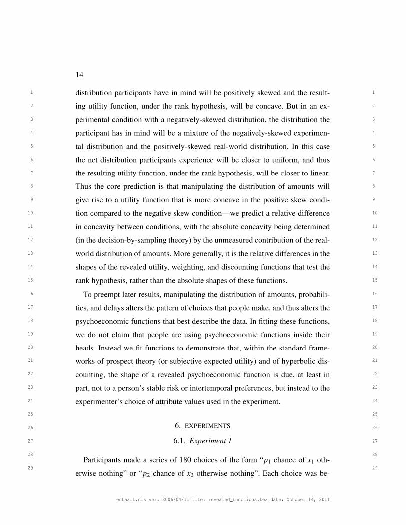
distribution participants have in mind will be positively skewed and the result-

ing utility function, under the rank hypothesis, will be concave. But in an ex-

perimental condition with a negatively-skewed distribution, the distribution the

participant has in mind will be a mixture of the negatively-skewed experimen-

tal distribution and the positively-skewed real-world distribution. In this case

the net distribution participants experience will be closer to uniform, and thus

the resulting utility function, under the rank hypothesis, will be closer to linear.

Thus the core prediction is that manipulating the distribution of amounts will

give rise to a utility function that is more concave in the positive skew condi-

tion compared to the negative skew condition—we predict a relative difference

in concavity between conditions, with the absolute concavity being determined

(in the decision-by-sampling theory) by the unmeasured contribution of the real-

world distribution of amounts. More generally, it is the relative differences in the

shapes of the revealed utility, weighting, and discounting functions that test the

rank hypothesis, rather than the absolute shapes of these functions.

To preempt later results, manipulating the distribution of amounts, probabili-

ties, and delays alters the pattern of choices that people make, and thus alters the

psychoeconomic functions that best describe the data. In fitting these functions,

we do not claim that people are using psychoeconomic functions inside their

heads. Instead we fit functions to demonstrate that, within the standard frame-

works of prospect theory (or subjective expected utility) and of hyperbolic dis-

counting, the shape of a revealed psychoeconomic function is due, at least in

part, not to a person’s stable risk or intertemporal preferences, but instead to the

experimenter’s choice of attribute values used in the experiment.

6. EXPERIMENTS

6.1. Experiment 1

Participants made a series of 180 choices of the form “p1 chance of x1 oth-

erwise nothing” or “p2 chance of x2 otherwise nothing”. Each choice was be-


15

1 1

2 2

3 3

4 4

5 5

6 6

7 7

8 8

9 9

10 10

11 11

12 12

13 13

14 14

15 15

16 16

17 17

18 18

19 19

20 20

21 21

22 22

23 23

24 24

25 25

26 26

27 27

28 28

29 29

tween a smaller probability of a larger amount or a larger probability of a smaller

amount. Between participants, the distribution of amounts available was manip-

ulated to be either positively skewed (as in the real world, Stewart, Chater, and

Brown, 2006) or negatively skewed.

6.1.1. Method

Participants

Forty one Warwick psychology first year undergraduates participated for course

credit. In addition, for each participant, two gambles were randomly selected to

be played for real money. Participants could win up to £5. Data from four par-

ticipants were deleted for violating stochastic dominance on more than 10% of

catch trials (see below), though including these data in the analysis does not alter

the pattern of results. Most participants in this experiment, and Experiments 2-4,

made no catch-trial errors.

Design

A set of 5 probabilities was crossed with a set of 6 amounts to create 30 gam-

bles of the form “p chance of x”. All participants experienced probabilities .2, .4,

.6, .8, and 1.0. Participants were randomly assigned to receive either a positively

or a negatively skewed set of amounts (see Figure 3, middle panel). The posi-

tively skewed set contained amounts £10, £20, £50, £100, £200, and £500. The

negatively skewed set was the mirror image of the positively skewed set with the

same range, and was constructed by subtracting each amount from £510.

The 30 gambles were crossed with themselves to create a set of choices.

Choices between identical gambles and choices where one gamble stochasti-

cally dominated the other were dropped to leave 150 choices between a small

probability of a large amount and a large probability of a small amount. In addi-

tion, 30 of the choices where one gamble stochastically dominated the other were

included as catch trials to detect participants who were not making considered


16

1 1

2 2

3 3

4 4

5 5

6 6

7 7

8 8

9 9

10 10

11 11

12 12

13 13

14 14

15 15

16 16

17 17

18 18

19 19

20 20

21 21

22 22

23 23

24 24

25 25

26 26

27 27

28 28

29 29

choices. All choices are given in Appendix A.

Procedure

Participants were tested individually. Written and spoken instructions explained

that participants would be asked to make a series of choices between pairs of

gambles. They were told to think of each gamble as an urn draw game in which

the urn contained 100 balls, with the percentage of winning balls matching the

percentage chance of winning the gamble. It was explained that drawing a win-

ning ball would result in receiving the amount in the gamble and that non-

winning balls would result in nothing. Participants were told that they would

randomly select two choices at the end of the experiment, with urn draws made

to determine their winnings, subject to an experiment exchange rate (which was

also applied in the other experiments). The amounts and probabilities on offer

were displayed in lists at the top of the screen to remind participants of the at-

tributes they would experience.

Each choice was presented as two buttons, one for each gamble. Each button

had text describing the gamble. For example, for one choice in the Positive-

Skew Condition, one button was labeled “60% chance of £200” and the other

was labeled “100% chance of £10”. The assignment of gamble to button was

made randomly on each trial. Participants clicked their preferred gamble with

the mouse. The next choice appeared automatically. The ordering of choices was

set randomly for each participant. A progress bar at the bottom of the screen

tracked the progress of the participant through the experiment.

At the end of the experiment, participants randomly selected two choices and

played their selected gambles. Participants kept their winnings subject to an ex-

periment exchange rate. Participants could win up to £5.


17

1 1

2 2

3 3

4 4

5 5

6 6

7 7

8 8

9 9

10 10

11 11

12 12

13 13

14 14

15 15

16 16

17 17

18 18

19 19

20 20

21 21

22 22

23 23

24 24

25 25

26 26

27 27

28 28

29 29

6.1.2. Results and Discussion

For each participant, raw data were 180 choices between pairs of gambles.

Two analyses were completed. The first is a nonparametric analysis and reveals

utility and weighting functions from the data without assuming a particular func-

tional form for either. The second is a parametric analysis and fits power law

utility functions for each participant.

Nonparametric Analysis

Equation 6.1 gives a model for the probability of picking the gamble displayed

on the right hand side of the screen as a function of the subjective expected utility

w(p)U(x) of each gamble. The weighting function w(p) converts the objective

probability p into its subjective equivalent. The utility function U(x) converts

money x into its subjective equivalent. Subscripts indicate left and right. The

Luce (1959)–Shepard (1957) choice formulation gives a high probability of se-

lecting the right gamble when it has a relatively higher subjective expected util-

ity. The γ parameter controls the degree of determinism in the model: γ = 1 gives

choice probabilities proportional to the subjective expected utilities and γ > 1

gives more extreme choice probabilities, so gambles with only slightly higher

subjective expected utility are very likely to be chosen.

(6.1) P(Right) =[w(pR)U(xR)]

γ

[w(pL)U(xL)]γ +[w(pR)U(xR)]

γ

The advantage of using this Luce formulation is that, when expressed as log

odds (Equation 6.2), the right hand side of the equation is linear in log subjective

values. This means that the subjective values of each probability and amount can

be straightforwardly estimated in a logistic regression.

(6.2) ln[

P(right)1−P(Right)

]= γ [lnw(pR)+ lnU(xR)− lnw(pL)− lnU(xL)]

Equation 6.3 rewrites Equation 6.2 in matrix notation. Each element in vector β

represents the (logarithm of the) subjective probability or value of each attribute


18

1 1

2 2

3 3

4 4

5 5

6 6

7 7

8 8

9 9

10 10

11 11

12 12

13 13

14 14

15 15

16 16

17 17

18 18

19 19

20 20

21 21

22 22

23 23

24 24

25 25

26 26

27 27

28 28

29 29

used. Each row in matrix X indicates which attributes are present for a given trial,

with -1 marking the presence of an attribute in the left hand gamble, 1 marking

the presence of an attribute in the right hand gamble, and 0 the absence of an

attribute from that trial. Each element in vector p represents the probability of

responding right, P(Right), for each trial.

(6.3) ln[

p1−p

]= X.β

Thus standard logistic regression can be used to obtain the maximum likelihood

estimate of β. In this way, the subjective probability associated with each prob-

ability and the subjective utility of each amount in the experiment are obtained

without assuming any functional forms for weighting or utility functions. With-

out loss of generality, the utility of £500 was set at 1, and the subjective proba-

bility of 100% was set at 1.

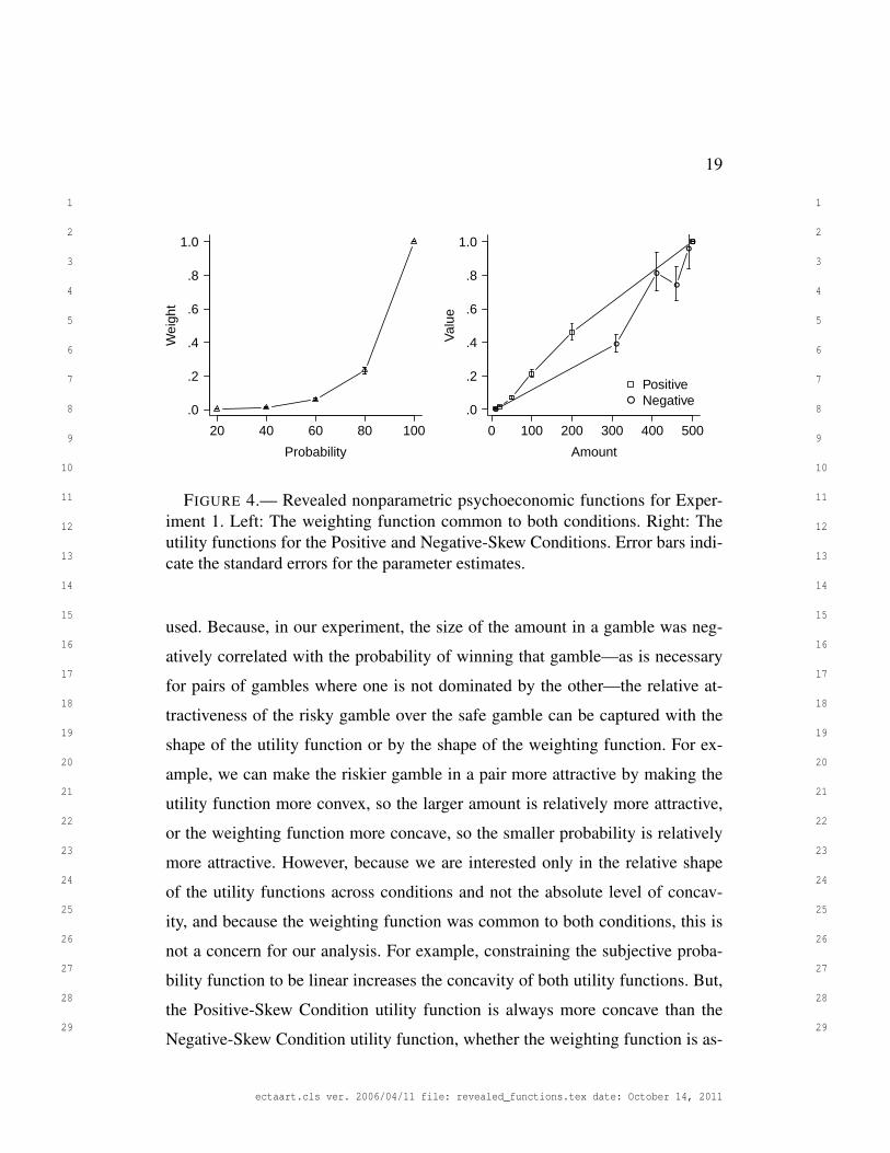
The revealed utility functions are shown in Figure 4. Effectively, the logis-

tic regression adjusted the heights of each point in the weighting function and

utility functions to best fit the choices participants made. Though they were not

constrained to do so functions increase monotonically, with the exception of one

utility. The utility function for the Positive-Skew Condition is concave, whereas

the utility function for the Negative-Skew Condition is convex. Parameter stan-

dard errors indicate that the functions differ significantly. And this is the core

result: Participants who experienced a different distribution of amounts behaved

as if they had a different shaped utility function.

The left panel shows the weighting function, which was assumed to be com-

mon to both conditions. The function has a convex shape (cf. the inverse-S shape

commonly found, Abdellaoui, 2000; Bleichrodt and Pinto, 2000; Gonzalez and

Wu, 1999; Kahneman and Tversky, 1979; Prelec, 1998; Tversky and Kahne-

man, 1992; Wu and Gonzalez, 1996, 1999). Experimenting with the model fitting

shows that there is some degree of trade-off between the shape of the weighting

function and the shapes of the utility functions when such simple choices are


19

1 1

2 2

3 3

4 4

5 5

6 6

7 7

8 8

9 9

10 10

11 11

12 12

13 13

14 14

15 15

16 16

17 17

18 18

19 19

20 20

21 21

22 22

23 23

24 24

25 25

26 26

27 27

28 28

29 29

20 40 60 80 100

Probability

Wei

ght

.0

.2

.4

.6

.8

1.0

0 100 200 300 400 500

AmountV

alue

.0

.2

.4

.6

.8

1.0

●

●

●

●

●

●

●

PositiveNegative

FIGURE 4.— Revealed nonparametric psychoeconomic functions for Exper-iment 1. Left: The weighting function common to both conditions. Right: Theutility functions for the Positive and Negative-Skew Conditions. Error bars indi-cate the standard errors for the parameter estimates.

used. Because, in our experiment, the size of the amount in a gamble was neg-

atively correlated with the probability of winning that gamble—as is necessary

for pairs of gambles where one is not dominated by the other—the relative at-

tractiveness of the risky gamble over the safe gamble can be captured with the

shape of the utility function or by the shape of the weighting function. For ex-

ample, we can make the riskier gamble in a pair more attractive by making the

utility function more convex, so the larger amount is relatively more attractive,

or the weighting function more concave, so the smaller probability is relatively

more attractive. However, because we are interested only in the relative shape

of the utility functions across conditions and not the absolute level of concav-

ity, and because the weighting function was common to both conditions, this is

not a concern for our analysis. For example, constraining the subjective proba-

bility function to be linear increases the concavity of both utility functions. But,

the Positive-Skew Condition utility function is always more concave than the

Negative-Skew Condition utility function, whether the weighting function is as-


20

1 1

2 2

3 3

4 4

5 5

6 6

7 7

8 8

9 9

10 10

11 11

12 12

13 13

14 14

15 15

16 16

17 17

18 18

19 19

20 20

21 21

22 22

23 23

24 24

25 25

26 26

27 27

28 28

29 29

sumed to be concave, convex, or linear.

Do these effects depend on extensive experience with the distributions? We do

not think so. Splitting the data for each participant into the first and second halves

of the experiment and conducting the analysis separately for each half (for this

and later experiments) revealed the same sized effect. This is unsurprising, given

attribute distribution effects can take place in as few as 10 trials (Stewart, 2009)

or after purchasing a few items in a shop (Ungemach, Stewart, and Reimers,

2011).

Parametric Analysis

The advantage of the nonparametric analysis is that it does not impose a par-

ticular functional form on the psychoeconomic functions. A drawback is that

data are treated as if all trials come from a single participant. The parametric

analysis here has the opposite properties, and imposes a functional form in fit-

ting a power-law function for each participant, and then compares parameters for

that power law across conditions. To preempt the results, the same conclusion is

reached—that people choose as if they have different utility functions in different

conditions.

(6.4) U(x) = xα

In fitting the data for each participant, utility is assumed to be a power function

of amount (Equation 6.4). When α < 1, the utility function is concave. When

α = 1 the utility function is linear. When α > 1, the utility function is convex.

The choice of a power function is not a theoretical statement from us about the

nature of the utility function—it is just a simple function that we can use to fit

the data and we would anticipate a very similar result if a different function were

used. The weighting function is assumed to be the identity function, so the model

reduces to expected utility. Note though that very similar results are obtained

if different forms for the weighting function are assumed. The probability of


21

1 1

2 2

3 3

4 4

5 5

6 6

7 7

8 8

9 9

10 10

11 11

12 12

13 13

14 14

15 15

16 16

17 17

18 18

19 19

20 20

21 21

22 22

23 23

24 24

25 25

26 26

27 27

28 28

29 29

0 100 200 300 400 500

Amount

Val

ue

.0

.2

.4

.6

.8

1.0

PositiveNegative

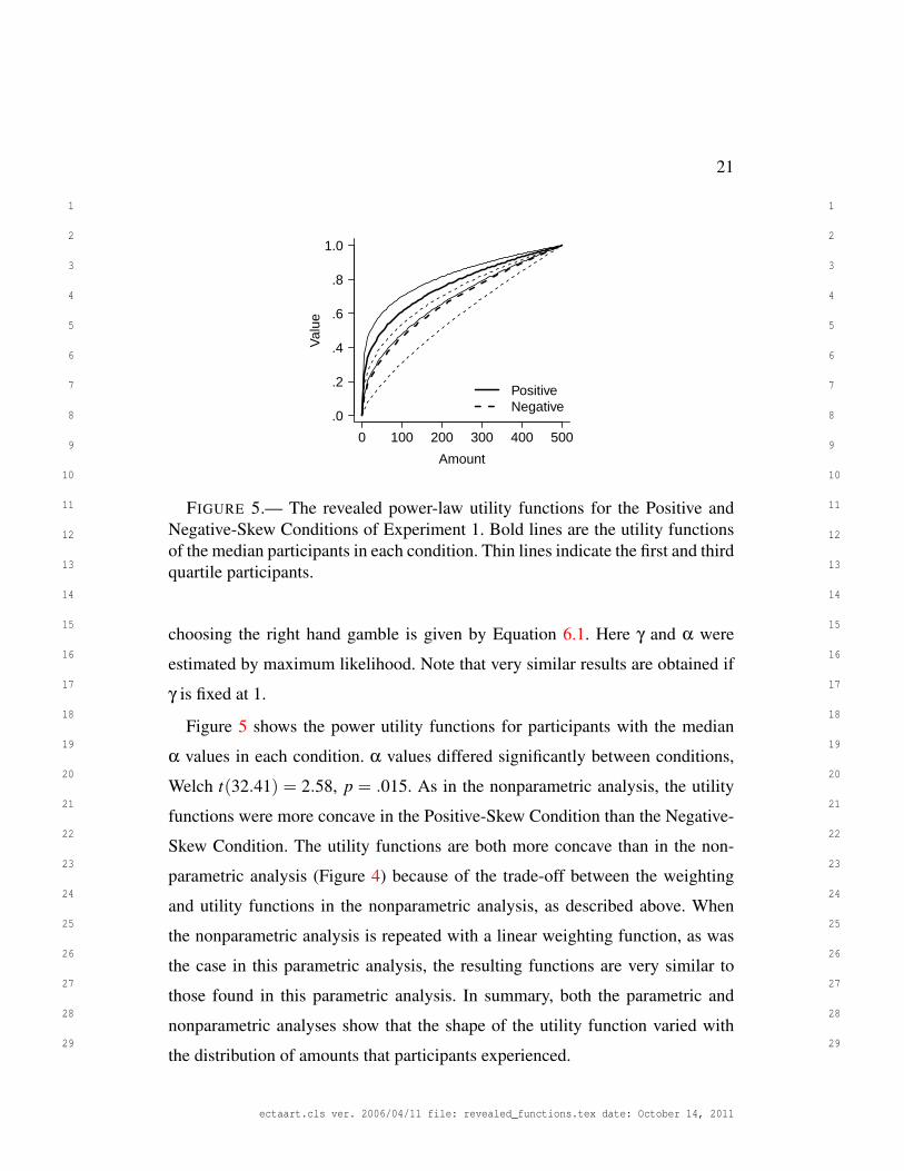
FIGURE 5.— The revealed power-law utility functions for the Positive andNegative-Skew Conditions of Experiment 1. Bold lines are the utility functionsof the median participants in each condition. Thin lines indicate the first and thirdquartile participants.

choosing the right hand gamble is given by Equation 6.1. Here γ and α were

estimated by maximum likelihood. Note that very similar results are obtained if

γ is fixed at 1.

Figure 5 shows the power utility functions for participants with the median

α values in each condition. α values differed significantly between conditions,

Welch t(32.41) = 2.58, p = .015. As in the nonparametric analysis, the utility

functions were more concave in the Positive-Skew Condition than the Negative-

Skew Condition. The utility functions are both more concave than in the non-

parametric analysis (Figure 4) because of the trade-off between the weighting

and utility functions in the nonparametric analysis, as described above. When

the nonparametric analysis is repeated with a linear weighting function, as was

the case in this parametric analysis, the resulting functions are very similar to

those found in this parametric analysis. In summary, both the parametric and

nonparametric analyses show that the shape of the utility function varied with

the distribution of amounts that participants experienced.


22

1 1

2 2

3 3

4 4

5 5

6 6

7 7

8 8

9 9

10 10

11 11

12 12

13 13

14 14

15 15

16 16

17 17

18 18

19 19

20 20

21 21

22 22

23 23

24 24

25 25

26 26

27 27

28 28

29 29

6.2. Experiment 2

6.2.1. Method

In Experiment 2 the distribution of probabilities was manipulated between

participants and the distribution of amounts was held constant. In other respects,

the method was the same as Experiment 1.

Participants

Thirty five Warwick psychology first year undergraduates participated for course

credit. In addition, participants knew they could win up to £5 performance-

related pay as in Experiment 1. No participants violated stochastic dominance

on more than 10% of catch trials, so all data were retained.

Design

Gambles were made by crossing a set of probabilities with a set of amounts.

The amounts were £100, £200, £300, £400, and £500. The set of probabilities

was manipulated between participants (see Figure 3, left panel) and was ei-

ther positively skewed (10%, 20%, 30%, 40%, 70%, 90%) or negatively skewed

(10%, 30%, 60%, 70%, 80%, 90%). The negatively skewed set is the mirror im-

age of the positively skewed set. Choices were made by crossing gambles. 120

non-stochastically dominated choices were selected at random and combined

with 30 stochastically dominated choices selected at random.

Procedure

Because probabilities were the focus of this experiment, we wanted to be sure

that participant understood the probabilities and the method for resolving them.

In this study, probabilities were resolved by drawing 1 of 100 chips from a bag.

To be successful, a number smaller than or equal to the probability (as a percent-

age) had to be drawn. For example, for a “70% chance £100” gamble, £100 was

received if one of the numbers 1-70 was drawn; numbers 71-100 led to no prize.


23

1 1

2 2

3 3

4 4

5 5

6 6

7 7

8 8

9 9

10 10

11 11

12 12

13 13

14 14

15 15

16 16

17 17

18 18

19 19

20 20

21 21

22 22

23 23

24 24

25 25

26 26

27 27

28 28

29 29

This procedure was explained to participants before they commenced the experi-

ment. The experimenter showed participants the chips in an ordered 10 x 10 grid,

sweeping their hands over the array to indicate, for several example probabilities,

which chips were winning chips. The participant then had the opportunity to ask

any questions before the experiment began.



The analysis repeats the procedure from Experiment 1, except subjective prob-

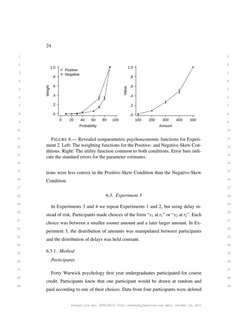
abilities instead of utilities varied between conditions. Figure 6 shows the re-

vealed weighting functions (left). Both functions are convex, but—and this is the

crucial result—the Positive-Skew Condition weighting function is less convex

than the Negative-Skew Condition weighting function. The probability 70% was

common to both conditions, but had a considerably higher subjective weight-

ing in the Positive Skew Condition compared to the Negative Skew Condition.

Effectively, people weight outcomes associated with 70% more heavily in the

Positive Skew Condition. The right panel shows the utility function common to

both conditions to be roughly linear.

Parametric Analysis

The nonparametric analysis suggest that a power law should be an adequate

parametric form to describe the weighting function (Equation 6.5). Adapting the

analysis for Experiment 1, φ and γ were estimated by maximum likelihood, with

a linear utility function assumed.

(6.5) w(p) = pφ

Figure 7 shows the power weighting functions for participants with the median φ

values in each condition. φ values differed marginally between conditions, Welch

t(26.93) = 1.82, p = .080. As in the nonparametric analysis, the weighting func-


24

1 1

2 2

3 3

4 4

5 5

6 6

7 7

8 8

9 9

10 10

11 11

12 12

13 13

14 14

15 15

16 16

17 17

18 18

19 19

20 20

21 21

22 22

23 23

24 24

25 25

26 26

27 27

28 28

29 29

0 20 40 60 80 100

Probability

Wei

ght

.0

.2

.4

.6

.8

1.0

● ●

●

●

●

●

●

PositiveNegative

100 200 300 400 500

AmountV

alue

.0

.2

.4

.6

.8

1.0

FIGURE 6.— Revealed nonparametric psychoeconomic functions for Experi-ment 2. Left: The weighting functions for the Positive- and Negative-Skew Con-ditions. Right: The utility function common to both conditions. Error bars indi-cate the standard errors for the parameter estimates.

tions were less convex in the Positive-Skew Condition than the Negative-Skew

Condition.

6.3. Experiment 3

In Experiments 3 and 4 we repeat Experiments 1 and 2, but using delay in-

stead of risk. Participants made choices of the form “x1 at t1” or “x2 at t2”. Each

choice was between a smaller sooner amount and a later larger amount. In Ex-

periment 3, the distribution of amounts was manipulated between participants

and the distribution of delays was held constant.

6.3.1. Method

Participants

Forty Warwick psychology first year undergraduates participated for course

credit. Participants knew that one participant would be drawn at random and

paid according to one of their choices. Data from four participants were deleted


25

1 1

2 2

3 3

4 4

5 5

6 6

7 7

8 8

9 9

10 10

11 11

12 12

13 13

14 14

15 15

16 16

17 17

18 18

19 19

20 20

21 21

22 22

23 23

24 24

25 25

26 26

27 27

28 28

29 29

0 20 40 60 80 100

Probability

Wei

ght

.0

.2

.4

.6

.8

1.0PositiveNegative

FIGURE 7.— The revealed power-law weighting functions for the Positive-and Negative-Skew Conditions of Experiment 2. Bold lines are the weightingfunctions of the median participant in each condition. Thin lines indicate the firstand third quartile participants. (Note that the almost straight line is the almostlinear weighting function for the lower-quartile participant in the Positive-SkewCondition, and is not a benchmark linear weighting function.)


26

1 1

2 2

3 3

4 4

5 5

6 6

7 7

8 8

9 9

10 10

11 11

12 12

13 13

14 14

15 15

16 16

17 17

18 18

19 19

20 20

21 21

22 22

23 23

24 24

25 25

26 26

27 27

28 28

29 29

for violating dominance on more than 10% of catch trials, though including these

data in the analysis does not alter the pattern of results.

Design

Delayed options were made by crossing a set of delays with a set of amounts.

All participants received delays of 1 day, 2 days, 1 week, 2 weeks, 1 month,

2 months, 6 months, and 1 year. The distribution of amounts was either posi-

tively or negatively skewed, with values from Experiment 1 (see Figure 3, mid-

dle panel). 120 non-dominated choices were selected at random and combined

with 30 stochastically dominated choices selected at random.

Procedure

Participants were told that one of them would be selected at random after the

experiment, that a choice would be randomly selected, and the winner would be

paid according to that choice by bank transfer on the relevant day in the future

(after applying an experiment exchange rate). Participants could win up to £20.



The analysis repeats the procedure from Experiment 1, with the subjective val-

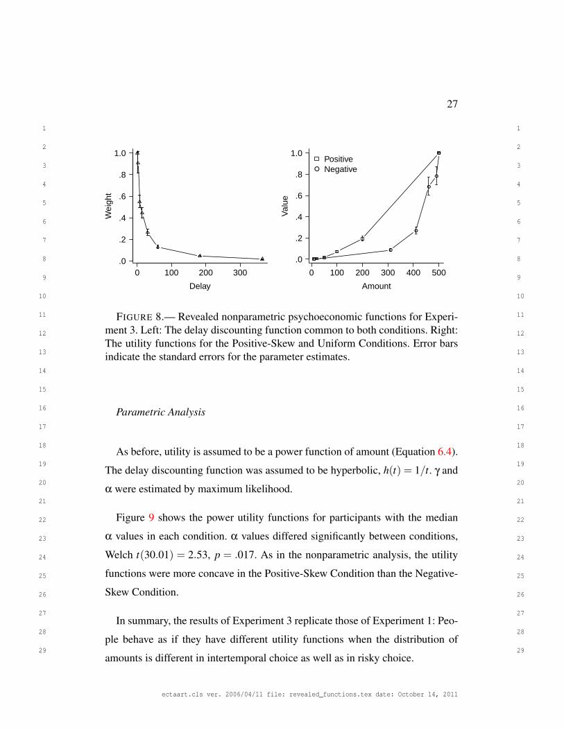
ues of amounts and times estimated by maximum likelihood. Figure 8 shows the

revealed delay discounting and utility functions. The delay discounting function

(left) shows a typical hyperbolic-like form. The utility functions (right) differ

between conditions. The utility function for the Positive-Skew Condition is rel-

atively linear, whereas the utility function for the Negative-Skew Condition is

convex. Crucially, the difference in the utility functions is in the direction ex-

pected: the function is more convex in the Negative-Skew Condition than the

Positive-Skew Condition.


27

1 1

2 2

3 3

4 4

5 5

6 6

7 7

8 8

9 9

10 10

11 11

12 12

13 13

14 14

15 15

16 16

17 17

18 18

19 19

20 20

21 21

22 22

23 23

24 24

25 25

26 26

27 27

28 28

29 29

0 100 200 300

Delay

Wei

ght

.0

.2

.4

.6

.8

1.0

0 100 200 300 400 500

AmountV

alue

.0

.2

.4

.6

.8

1.0

●

●

●

●

●

●

●

PositiveNegative

FIGURE 8.— Revealed nonparametric psychoeconomic functions for Experi-ment 3. Left: The delay discounting function common to both conditions. Right:The utility functions for the Positive-Skew and Uniform Conditions. Error barsindicate the standard errors for the parameter estimates.

Parametric Analysis

As before, utility is assumed to be a power function of amount (Equation 6.4).

The delay discounting function was assumed to be hyperbolic, h(t) = 1/t. γ and

α were estimated by maximum likelihood.

Figure 9 shows the power utility functions for participants with the median

α values in each condition. α values differed significantly between conditions,

Welch t(30.01) = 2.53, p = .017. As in the nonparametric analysis, the utility

functions were more concave in the Positive-Skew Condition than the Negative-

Skew Condition.

In summary, the results of Experiment 3 replicate those of Experiment 1: Peo-

ple behave as if they have different utility functions when the distribution of

amounts is different in intertemporal choice as well as in risky choice.


28

1 1

2 2

3 3

4 4

5 5

6 6

7 7

8 8

9 9

10 10

11 11

12 12

13 13

14 14

15 15

16 16

17 17

18 18

19 19

20 20

21 21

22 22

23 23

24 24

25 25

26 26

27 27

28 28

29 29

0 100 200 300 400 500

Amount

Val

ue

.0

.2

.4

.6

.8

1.0PositiveNegative

FIGURE 9.— The revealed power-law utility functions for the Positive andNegative-Skew Conditions of Experiment 3. Bold lines are the utility functionsof the median participant in each condition. Thin lines indicate the first and thirdquartile participants.

6.4. Experiment 4

6.4.1. Method

In Experiment 4 the distribution of delays was manipulated and the distribu-

tion of amounts was held constant. In all other respects, the method was the same

as Experiment 3.

Participants

Thirty Warwick psychology first year undergraduates participated for course

credit. Participants knew that one participant would be drawn at random and

paid according to one of their choices. Data from five participants were deleted

for violating dominance on more than 10% of catch trials, though including these

data in the analysis does not alter the pattern of results.


29

1 1

2 2

3 3

4 4

5 5

6 6

7 7

8 8

9 9

10 10

11 11

12 12

13 13

14 14

15 15

16 16

17 17

18 18

19 19

20 20

21 21

22 22

23 23

24 24

25 25

26 26

27 27

28 28

29 29

Design

Gambles were made by crossing a set of probabilities with a set of amounts.

The amounts were £100, £200, £300, £400, and £500. The set of delays was

manipulated between participants (see Figure 3, right panel) and was either posi-

tively skewed (1 day, 2 days, 1 week, 2 weeks, 1 month, 2 months, 6 months, and

1 year) or uniformly distributed (1 day, 2 months, 4 months, 6 months, 8 months,

10 months, and 1 year).



The analysis repeats the procedure from earlier experiments, with weightings

of delays allowed to vary between conditions and utilities held constant across

conditions. Figure 10 shows the revealed delay discounting functions (left). The

delay discounting function is initially much steeper in the Positive-Skew Con-

dition and much closer to linear in the Uniform Condition. For the common 2-

month and 6-month delays, people behaved as if they weighted delayed amounts

less heavily in the Positive Skew Condition compared to the Uniform Condi-

tion. The right panel shows the utility function common to both conditions to be

convex.

Parametric Analysis

We use the standard hyperbolic functional form for fitting delay discounting

data (Equation 6.6). k and γ were estimated by maximum likelihood, with a linear

utility function assumed.

(6.6) h(t) = 1/(1+ kt)

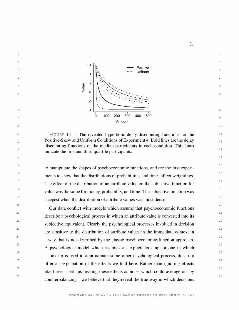
Figure 11 shows the hyperbolic discounting functions for participants with the

median k values in each condition. k values differed significantly between con-

ditions, Welch t(13.93) = 2.21, p = .044. As in the nonparametric analysis, the


30

1 1

2 2

3 3

4 4

5 5

6 6

7 7

8 8

9 9

10 10

11 11

12 12

13 13

14 14

15 15

16 16

17 17

18 18

19 19

20 20

21 21

22 22

23 23

24 24

25 25

26 26

27 27

28 28

29 29

0 100 200 300

Delay

Wei

ght

.0

.2

.4

.6

.8

1.0 ●

●

●

●● ● ●

●

PositiveUniform

100 200 300 400 500

AmountV

alue

.0

.2

.4

.6

.8

1.0

FIGURE 10.— Revealed nonparametric psychoeconomic functions for Exper-iment 4. Left: The delay discounting functions for the Positive-Skew and Uni-form Conditions. Right: The utility function common to both conditions. Errorbars indicate the standard errors for the parameter estimates.

delay discounting function was initially steeper in the Positive-Skew Condition

and more linear in the Uniform Condition.

7. GENERAL DISCUSSION

Experimentally manipulating the distribution of monies, probabilities, and de-

lays people experience alters the choices people make, which in turn alters the

psychoeconomic functions constructed to describe those choices. In Experiments

1 and 3, for risky and intertemporal choices, the revealed utility function translat-

ing money into its subjective equivalent was more concave when the distribution

of money was positively skewed rather than negatively skewed. In Experiment

2, for risky choices, the revealed weighting function was more concave when

the distribution of probabilities was positively skewed rather than negatively

skewed. In Experiment 4, for intertemporal choices, the revealed discounting

function was more convex when the distribution of delays was positively skewed

rather than uniformly distributed. We believe that these are the first experiments


31

1 1

2 2

3 3

4 4

5 5

6 6

7 7

8 8

9 9

10 10

11 11

12 12

13 13

14 14

15 15

16 16

17 17

18 18

19 19

20 20

21 21

22 22

23 23

24 24

25 25

26 26

27 27

28 28

29 29

0 100 200 300 400 500

Amount

Val

ue

.0

.2

.4

.6

.8

1.0PositiveUniform

FIGURE 11.— The revealed hyperbolic delay discounting functions for thePositive-Skew and Uniform Conditions of Experiment 4. Bold lines are the delaydiscounting functions of the median participants in each condition. Thin linesindicate the first and third quartile participants.

to manipulate the shapes of psychoeconomic functions, and are the first experi-

ments to show that the distributions of probabilities and times affect weightings.

The effect of the distribution of an attribute value on the subjective function for

value was the same for money, probability, and time: The subjective function was

steepest when the distribution of attribute values was most dense.

Our data conflict with models which assume that psychoeconomic functions

describe a psychological process in which an attribute value is converted into its

subjective equivalent. Clearly the psychological processes involved in decision

are sensitive to the distribution of attribute values in the immediate context in

a way that is not described by the classic psychoeconomic-function approach.

A psychological model which assumes an explicit look up, or one in which

a look up is used to approximate some other psychological process, does not

offer an explanation of the effects we find here. Rather than ignoring effects

like these—perhaps treating these effects as noise which could average out by

counterbalancing—we believe that they reveal the true way in which decisions


32

1 1

2 2

3 3

4 4

5 5

6 6

7 7

8 8

9 9

10 10

11 11

12 12

13 13

14 14

15 15

16 16

17 17

18 18

19 19

20 20

21 21

22 22

23 23

24 24

25 25

26 26

27 27

28 28

29 29

are constructed, on-the-fly, using simple cognitive tools.

Sometimes economists are not interested in psychological processes. They

present their models as “as if” models, where although people’s behavior is con-

sistent with the mathematical model, people are not necessarily assumed to be

implementing the calculations in the model. Our data also constrict these “as if”

models. Our finding that the distribution of attribute values changes the shape of

utility, weighting, and discounting functions limits the descriptive power of the

models, because different psychoeconomic functions would be needed for each

different choice set. Thus functions revealed in a particular context will not apply

in new contexts, reducing the generalizability of the theories. Instead of having

a single psychoeconomic function for money, a single psychoeconomic function

for probability, and a single psychoeconomic function for delay, a large set of

functions would be needed, one for each context. That is, a single function is

not a sufficient description of people’s choices. Instead a whole set of functions

is required, together with a theory to map functions to contexts with different

attribute value distributions.

Random utility models (Becker, DeGroot, and Marschak, 1963; see Loomes,

2005, for recent discussion) may seem like an obvious way of accommodating

the present results. In a random utility model, the decision maker is assumed to

have a set of different utility functions, from which one is randomly selected each

time a decision is made (typically, one or more of the parameters of the utility

function are assumed to be random variables). These models are intended to

account for trial-to-trial variability in the decisions people make (see Blavatskyy

and Pogrebna, 2010, for tests of these models). An account of the present results

might go as follows: The utility functions drawn could differ across contexts

with different attribute-value distributions. What would be required is a theory

providing a parsimonious link between the attribute-value distributions in a given

context and the set of utility functions available in that context. Such a theory

could be descriptive: that is, it could accommodate the effects of attribute-value


33

1 1

2 2

3 3

4 4

5 5

6 6

7 7

8 8

9 9

10 10

11 11

12 12

13 13

14 14

15 15

16 16

17 17

18 18

19 19

20 20

21 21

22 22

23 23

24 24

25 25

26 26

27 27

28 28

29 29

distributions without explaining how they arise. For example, range-frequency

theory might play some role here. But it could go further and explain why the sets

of utility functions available differ across contexts with different attribute-value

distributions. We offer the decision-by-sampling theory as one candidate here: it

suggests that, in the absence of stable internal mappings between attribute values

and their subjective equivalents, people are forced to derive subjective values on

the fly from a series of comparisons with attribute values they have in mind.

In the context of random utility models, the set of available utility functions

would be constructed for a particular context, with the variability coming from

stochastic components of the memory and comparison processes.

Our experimental results also have implications for the process by which theo-

ries of decision under risk and delay are developed. Over the past half century, a

considerable literature has been amassed. There are many competing models of

decision under risk with, typically, each model accounting for some experimen-

tal demonstration of departure from expected utility theory (or prospect theory)

or discounted utility theory (or hyperbolic discounting theory). Violations of var-

ious axioms of expected or discounted utility theory leads to the development of

new models which are based upon alternative axiomatic formulations. Models

are also selected on their ability to fit choice data from benchmark data sets. Re-

cently, Brandstatter, Gigerenzer, and Hertwig (2006), Birnbaum (2008), Loomes

(2010), and Scholten and Read (2010) have published major theory papers using

exactly these methodologies. (Note though that Brandstatter et al.’s model is a

set of heuristics, and Loomes’s and Scholten and Read’s models concerns trade-

offs between attribute values, rather than independent valuation of each option.

That is, these models don’t follow the standard expected utility or discounted

utility frameworks.) Our finding that revealed psychoeconomic functions are not

stable presents two problems for this approach. First, axiomatic violations may

hold only for certain contexts with particular distributions of attribute values. Of

course, any violation rejects a particular model, but an understanding of which


34

1 1

2 2

3 3

4 4

5 5

6 6

7 7

8 8

9 9

10 10

11 11

12 12

13 13

14 14

15 15

16 16

17 17

18 18

19 19

20 20

21 21

22 22

23 23

24 24

25 25

26 26

27 27

28 28

29 29

distributions lead to which violations will be important in understanding why

some models do well in some analyses and badly in others. Second, compe-

titions between models may generalize poorly. Typically competitions involve

many choices, and sometimes hundreds of choices, and thus a quite dense and

broad distribution of attribute values. Models which perform well in this context

may generalize badly to real-world decisions where single choices are made in

relatively isolated contexts (apart from in the special case where the distribution

of attribute values in the experiment matches the distribution in a participant’s

memory).

The effects of manipulating the distribution of attribute values are not as com-

plete as would be predicted from the differences in the distributions used in our

experiments alone. For example, compare the predicted effect of changing the

skew of the distribution of amounts from positive to negative in Figure 3 with the

data from Experiments 1 and 3 (Figures 4, 5, 8, and 9). The experimental effects

are a little smaller than the predicted effect. One possibility, discussed earlier, is

that participants brought to the experiment a background distribution of attribute

values from everyday life. This background distribution is probably positively

skewed (Stewart, Chater, and Brown, 2006), and would act to dilute the effects

of the experimental distributions, making both utility functions more concave.

Another possibility is that people do possess some crude underlying transforma-

tion between attribute values and their subjective equivalents, but this underlying

transformation is extremely malleable. Irrespective of which of these accounts is

correct, we advocate abandoning the lookup approach to decision making and

we will continue to bring factors affecting the valuation of economic attributes

under experimental control.

7.1. Not Just Another Context / Choice Set Effect

The literature on choices between gambles documents many context or choice

set effects and other violations of expected utility theory. Typically one of two


35

1 1

2 2

3 3

4 4

5 5

6 6

7 7

8 8

9 9

10 10

11 11

12 12

13 13

14 14

15 15

16 16

17 17

18 18

19 19

20 20

21 21

22 22

23 23

24 24

25 25

26 26

27 27

28 28

29 29

fixes is offered. The first type of fix is a change of psychological primitive. For

example, in the endowment effect merely possessing a good makes it more valu-

able (Kahneman, Knetsch, and Thaler, 1991). The explanation proposed, loss

aversion, suggests that people are sensitive to changes (gains and losses) and not

final wealth states. As another example, sensitivity to branch splitting suggests

people reason with risk-reward branches and not cumulative probability distri-

butions (Birnbaum, 2008). The second type of fix is to assume more complexity

in the transformation of objective into subjective values. For example, the four-

fold pattern of risk seeking for large losses, risk aversion for small losses, risk

aversion for large losses, and risk aversion for large gains and risk seeking for

small gains (Kahneman and Tversky, 1979) motivated the inverse-S-shape of the

weighting function.

The effects we present here are different. Rather than supporting a change in

the shape of a utility, weighting, or discounting function, or a change in the pri-

mates which people process, our data suggest that the whole enterprise of using

stable functions to translate between objective and subjective values should be

abandoned. Theories based around the expected or discounted utility framework

are refuted: Descriptively, it is not adequate merely to propose separate functions

for each possible context without providing a theory mapping the distribution to

the shape of the psychoeconomic function. Psychologically, the translation be-

tween objective and subjective values does not represent a process taking place

in people’s heads.

Is the effect we report large enough that it should be of concern? Our data

show that the effect of context here is about as large as the individual differences

between people. Figures 5, 7, 9, and 11 show that the difference between the

median participants in each condition is about as large as the interquartile range

within each condition. If individual differences in, for example, risk aversion are

of concern, then we argue that the similar sized effect of context should also be

of concern.


36

1 1

2 2

3 3

4 4

5 5

6 6

7 7

8 8

9 9

10 10

11 11

12 12

13 13

14 14

15 15

16 16

17 17

18 18

19 19

20 20

21 21

22 22

23 23

24 24

25 25

26 26

27 27

28 28

29 29

7.2. Previous Investigations of the Shapes of Utility, Weighting, andDiscounting Functions

Here, we illustrate how classic studies in which utility, weighting, and dis-

counting are actually set up with attribute value distributions that produce the

classic shapes. The essential observation here is that, quite sensibly, functions

are typically measured in more detail (i.e., at more closely spaced intervals)

where they are expected to change most quickly. Take, for example, the sem-

inal study by Gonzalez and Wu (1999) on the shapes of utility and weighting

functions. Just as we did here, Gonzalez and Wu inferred utility and weighting

functions from a series of choices. Gonzalez and Wu used choices between two-

branch gambles and sure amounts of money to determine a certainty equivalent

for each gamble. They then used a non-parametric method to estimate the utility

of each sum of money and the weighting of each probability from these certainty

equivalents, just as we did here. Figure 12 plots (open circles) the empirical util-

ity and weighting functions that Gonzalez and Wu recovered. The lines on the

plots show the functions predicted by decision by sampling assuming that the

set of gambles offered to participants provides the distribution of attribute val-

ues against which the amounts and probabilities were compared. For both the

utility and weighting functions, the functions predicted under this simple rank

hypothesis show the same qualitative pattern seen in the empirical functions re-

covered by Gonzalez and Wu: The utility function is concave and the weighting

function is inverse-S-shaped. Gonzalez and Wu presumably used more small

amounts than large amounts because previous research indicated that the utility

function varies more quickly over smaller amounts than large amounts so, for

accuracy, more measurements should be taken for smaller amounts. Thus there

is a self fulfilling result here: By taking more measurements of small amounts,

necessarily small amounts occur more often in the question set, which in turn

leads to a steeper utility function for smaller amounts. Similarly, Gonzalez and

Wu used more small and large probabilities than intermediate probabilities—


37

1 1

2 2

3 3

4 4

5 5

6 6

7 7

8 8

9 9

10 10

11 11

12 12

13 13

14 14

15 15

16 16

17 17

18 18

19 19

20 20

21 21

22 22

23 23

24 24

25 25

26 26

27 27

28 28

29 29

0.0 0.2 0.4 0.6 0.8 1.0

0.0

0.2

0.4

0.6

0.8

1.0

Probability

We

igh

t

0 200 400 600 800

01

02

03

04

0

AmountV

alu

e

FIGURE 12.— Empirically derived utility (left) and weighting (right) func-tions from Gonzalez and Wu (1999). Circles plot the functions Gonzalez and Wurecovered. The solid line plots the predictions of decision-by-sampling theory.

because previous research suggests the weighting function is steeper for small

and large probabilities and so should be measured more carefully—and thus find

a steeper weighting function for small and large probabilities than intermediate

probabilities.

The same logic can be applied to classic studies in intertemporal choice. Rach-

lin, Raineri, and Cross (1991) used hypothetical choices between an immediately

available sum of money and a delayed sum. Participants chose between a delayed

$1,000 and an immediate sure sum that was titrated up and then down. Then the

procedure was repeated for each delay. Figure 13 plots (open circles) the me-

dian immediate amount at which people swapped between choosing the delayed

$1,000 and the immediate amount. The line on the plot show the function pre-

dicted by decision by sampling assuming that the set of delays presented provides

the comparison set. As for the Gonzalez and Wu data, the function predicted un-

der this simple rank hypothesis show the same qualitative pattern seen in the

empirical function. The discounting function is roughly hyperbolic because of


38

1 1

2 2

3 3

4 4

5 5

6 6

7 7

8 8

9 9

10 10

11 11

12 12

13 13

14 14

15 15

16 16

17 17

18 18

19 19

20 20

21 21

22 22

23 23

24 24

25 25

26 26

27 27

28 28

29 29

●

●

●

●

●

●

●

0 100 200 300 400 500 600

020

040

060

080

010

00

Delay / months

Dis

coun

ted

Val

ue /

$

FIGURE 13.— An empirically derived discounting function from Rachlin,Raineri, and Cross (1991), showing the discounted value of a delayed $1,000.Circles plot the function Rachlin, Raineri, and Cross recovered. The solid lineplots the predictions of decision-by-sampling theory.

the geometrically spaced distribution of delays chosen by Rachlin, Raineri, and

Cross. Virtually all discounting studies that show hyperbolic (or any other kind

of) discounting use this kind of distribution of delays.

In summary, we have discussed four findings with one common explanation.

The findings are: (a) People behave in the real world as if they have concave util-

ity functions, inverse-S-shaped weighting functions, and hyperbolic discounting

functions. (b) People behave in the same way in experiments (as discussed here

and in Sections 2 and 3). (c) Changes in the real-world distribution of attribute

values cause changes in real world decisions (Section 4, Ungemach, Stewart, and

Reimers, 2011). (d) Changes in the distribution of attribute values used in experi-

ments cause changes in laboratory decisions (Experiments 1-4). Expected utility

theory and discounted utility theory and their derivatives do not explain any of

these results. Here we have argued that all of these findings are the result of the

interaction between the distribution of attribute values people have in mind and

the simple cognitive tool of binary ordinal comparison described in the decision


39

1 1

2 2

3 3

4 4

5 5

6 6

7 7

8 8

9 9

10 10

11 11

12 12

13 13

14 14

15 15

16 16

17 17

18 18

19 19

20 20

21 21

22 22

23 23

24 24

25 25

26 26

27 27

28 28

29 29

by sampling theory.

7.3. Utility

We finish with a consideration of the implications of our experimental results

for the concept of utility.

7.3.1. Cardinal utility

Bentham (1970) proposed the idea that the real numbers could be assigned to

the pain or pleasure brought by goods. This idea, labeled cardinal utility, still

remains in risky and intertemporal choice. For example, the idea is central to

the development of stochastic models of decision under risk which predict the

strength of preference as a function of the difference in utility (e.g., stochastic ex-

pected utility theory, Blavatskyy, 2007, and stochastic cumulative prospect the-

ory, Busemeyer, 1985; Erev, Roth, Slonim, and Barron, 2002). Our data present

a significant challenge to the cardinal utility approach, because the data are not

consistent with a stable mapping between money and the real numbers—the

mapping fluctuates between contexts with different distributions of money.

The notion that the subjective value of an attribute might depend on the dis-

tribution of attribute values has been incorporated into at least two significant

economic models of decision under risk. In Koszegi and Rabin’s (2006; 2007)

model, the utility of a particular amount is a combination of classical, consump-

tion utility and gain-loss utility. Gain-loss utility measures the discrepancy be-

tween a target amount and the outcomes people expect (see also disappointment

theory, Bell, 1985; Gul, 1991; Loomes and Sugden, 1986, where outcomes are

evaluated relative to the mean outcome expected rather than to the entire distri-

bution). Specifically, the difference between the target amount and a particular

expectation is transformed by a value function that is concave for positive values

(where the target amount exceeds the expectation) and convex for negative values

(cf. Kahneman and Tversky, 1979), and this transformation is integrated over the


40

1 1

2 2

3 3

4 4

5 5

6 6

7 7

8 8

9 9

10 10

11 11

12 12

13 13

14 14

15 15

16 16

17 17

18 18

19 19

20 20

21 21

22 22

23 23

24 24

25 25

26 26

27 27

28 28

29 29

distribution of expectations. This model accounts for a series of economic phe-

nomena beyond the expected utility model (e.g., people are willing to pay more

for a good that they expected to buy and people are less likely to continue to

work when income is higher than they expected). In a parallel but unrelated de-

velopment Maccheroni, Marinacci, and Rustichini (2009a,b) have also proposed

that the utility of a target amount depends upon a comparison with a reference

distribution. Here, the reference distribution is the set of outcomes experienced

by others. An agent’s utility is a combination of classical, subjective expected

utility and a position index which increases with the utility of the agent’s own

outcome and decreases with the distribution of the agents’ peers.

These models are related to the decision-by-sampling model (Stewart, Chater,

and Brown, 2006) described earlier, in which the subjective value of an amount

(or probability or delay) is just the rank position within the reference distribution.

Both Koszegi and Rabin and Maccheroni, Marinacci, and Rustichini assume an

additional, stable classical utility component. And Koszegi and Rabin assume

that their gain-loss utility is cardinal, rather than just the rank position in the

distribution. The models also differ on the source of the reference distribution:

Koszegi and Rabin assume the distribution is of (rational) expected outcomes,

Maccheroni, Marinacci, and Rustichini assume it is the outcomes of peers, and

Stewart, Chater, and Brown assume it is the attribute values in immediate mem-

ory, many of which are from the immediate context or are evoked from long-term

memory by the immediate context. This paper, and related work, provide exper-

imental and field evidence that it is the attribute values in mind that matter as

decision by sampling states—and these values could well include expected out-

comes or the outcomes of others.

7.3.2. Ordinal utility

Read (2007, see also Stigler, 1950a,b) gives a review of the historical shift

from Bentham’s cardinal utility to the modern ordinal utility approach. The


41

1 1

2 2

3 3

4 4

5 5

6 6

7 7

8 8

9 9

10 10

11 11

12 12

13 13

14 14

15 15

16 16

17 17

18 18

19 19

20 20

21 21

22 22

23 23

24 24

25 25

26 26

27 27

28 28

29 29

problem with Bentham’s approach is that the utility of a good is not indepen-

dent of other goods as is assumed in Bentham’s approach. For example, coffee

is more useful if one possesses an espresso machine. Edgworth proposed that

utility should be a function of the entire basket of goods one possesses. Pareto

demonstrated that all that is required for modern economics is that people can or-

der their preferences over baskets of goods. Baskets of goods can be represented

in a multidimensional space, with baskets between which the agent is indifferent

joined by contours of equal utility. Now utility is ordinal: All that is required for

modern economics is that, if one basket is preferred to another, then it comes

from a higher indifference curve. Preferences are said to be revealed. Numbers

attached to the contours are only ordinal and are arbitrary as long as higher in-

difference curves are assigned higher numbers. The difference between utilities

has no meaning, and thus any monotonic transformation of a utility function

is permitted. Given our experimental manipulations do not change the ordering

of utilities—utility curves always increase monotonically—one might argue that

these data do not present a problem for the modern economic approach.

But we believe our results are still important for modern economics. Essen-

tially, risky choice can be viewed as choice between baskets of risk and reward,

where one basket might contain a large reward and a large risk whereas an-

other might contain a smaller reward at smaller risk. Intertemporal choice can

be viewed in the same way. Our results suggest that it should be possible to

observe a reversal of the preference between two “baskets” in difference con-

texts. This is just the result found by Stewart (2009) and Ungemach, Stewart,

and Reimers (2011) described earlier (see also Dorlet, Simonson, and Tversky,

2000). Thus the notion that people have stable preferences between baskets of

goods is, empirically, not true.


42

1 1

2 2

3 3

4 4

5 5

6 6

7 7

8 8

9 9

10 10

11 11

12 12

13 13

14 14

15 15

16 16

17 17

18 18

19 19

20 20

21 21

22 22

23 23

24 24

25 25

26 26

27 27

28 28

29 29

7.3.3. Neuroeconomic evidence

Our experimental results are consistent with recent evidence of coding of rel-

ative value within the brain. Seymour and McClure (2008) give a recent review.

For example, Tremblay and Schultz (1999) recorded from single cells in the

macaque orbitofrontal cortex. Cells fired more strongly on presentation of a piece

of apple as a reward when the other available reward was a piece of cereal (which

monkeys do not like that much) compared to when the other available reward was

a raisin (which monkeys love): The value of the apple was coded relative to the

other available rewards.

Some studies in neuroeconomics seem to provide compelling evidence for

utility or value functions. For example, Tom, Fox, Trepel, and Poldrack (2007)

showed that regions of the striatum and VMPFC show conjoint positive sensitiv-

ity to increases in the size of a gain and decreases in the size of a loss. Further,

the majority of individuals showed loss aversion: the increase in activity for a

given gain was about half the decrease in activity for the same sized loss. Tom,

Fox, Trepel, and Poldrack argue that they have uncovered the neural basis of the

value function and loss aversion. But this evidence is completely consistent with

our rank-based explanation of the present data. Tom, Fox, Trepel, and Poldrack

used gains in the range $10 to $40, but losses in the range $5 to $20 in their

experiment. Thus finding that people are twice as sensitive to losses is entirely

expected given the distribution of losses spans only half the range that the dis-

tribution of gains covers. What is required to demonstrate the existence of stable

value functions would be to show that the brain activation for a particular gain (or

loss) is invariant across a set of contexts. To our knowledge, such an experiment

has not been done.

7.4. Conclusion

To close, if we can measure lots of utility functions, which utility function is

the right one? Alternatively, if one infers a level of risk aversion from a series of


43

1 1

2 2

3 3

4 4

5 5

6 6

7 7

8 8

9 9

10 10

11 11

12 12

13 13

14 14

15 15

16 16

17 17

18 18

19 19

20 20

21 21

22 22

23 23

24 24

25 25

26 26

27 27

28 28

29 29

choices, whether in an experimental setting or by observing real-world decision,

which choices reveal the “true” level of risk aversion? One can pose similar ques-

tions for weighting and discounting functions. The answer, we fear, is that there

is no method which gives, even with careful counterbalancing, the true level of

risk aversion or the true shape of a utility function. In any given situation, one

can observe choices and infer a shape or level of risk aversion. But as soon as

the context changes—that is, as soon as the decision maker experiences any new

amount—the measured shape or level of risk aversion will no longer apply. Sim-

ilarly, one cannot examine risk aversion in one market situation and generalize to

another. Bluntly: individuals do not have utility functions with particular shapes

and thus particular levels of risk aversion. If it is meaningful to talk of utility or

risk aversion at all, it is only in the instantaneous interaction between the distri-

bution of attribute values in the immediate context and the decision maker.

Yet laboratory experiments and observations from the field consistently sug-

gest concave utility functions, inverse-S-shaped probability weighting functions,

and hyperbolic-like discounting functions. Here we have offered the decision by

sampling theory as an explanation of these findings: The interaction between the

distribtion of gains, losses, risks, and delays in the world (or the laboratory) with

the simple cognitive tools of sampling from memory, binary ordinal comparison,

and frequency accumulation gives the ubiquitous psychoeconomic functions. We

have presented four laboratory experiments testing this account: Systematic ma-

nipulation of the distributions of gains, risks, and delays gives large and sys-

tematic change in the utility, weighting, and discounting functions revealed from

people’s choices. Decision by sampling provides a common account of the ori-

gin of utility, weighting, and discounting functions—and the explanation of how

we, as architects of the environment in which decisions were made, were able to

change their shapes.

APPENDIX A: CHOICES


44

1 1

2 2

3 3

4 4

5 5

6 6

7 7

8 8

9 9

10 10

11 11

12 12

13 13

14 14

15 15

16 16

17 17

18 18

19 19

20 20

21 21

22 22

23 23

24 24

25 25

26 26

27 27

28 28

29 29

Table A.1: Experiment 1 Choices

Positive Skew Negative SkewID p x q y p x q y1 20% £20 40% £10 20% £310 40% £102 20% £20 60% £10 20% £310 60% £103 20% £20 80% £10 20% £310 80% £104 20% £20 100% £10 20% £310 100% £105 40% £20 60% £10 40% £310 60% £106 40% £20 80% £10 40% £310 80% £107 40% £20 100% £10 40% £310 100% £108 60% £20 80% £10 60% £310 80% £109 60% £20 100% £10 60% £310 100% £1010 80% £20 100% £10 80% £310 100% £1011 20% £50 40% £10 20% £410 40% £1012 20% £50 60% £10 20% £410 60% £1013 20% £50 80% £10 20% £410 80% £1014 20% £50 100% £10 20% £410 100% £1015 20% £50 40% £20 20% £410 40% £31016 20% £50 60% £20 20% £410 60% £31017 20% £50 80% £20 20% £410 80% £31018 20% £50 100% £20 20% £410 100% £31019 40% £50 60% £10 40% £410 60% £1020 40% £50 80% £10 40% £410 80% £1021 40% £50 100% £10 40% £410 100% £1022 40% £50 60% £20 40% £410 60% £31023 40% £50 80% £20 40% £410 80% £31024 40% £50 100% £20 40% £410 100% £31025 60% £50 80% £10 60% £410 80% £1026 60% £50 100% £10 60% £410 100% £1027 60% £50 80% £20 60% £410 80% £31028 60% £50 100% £20 60% £410 100% £31029 80% £50 100% £10 80% £410 100% £1030 80% £50 100% £20 80% £410 100% £31031 20% £100 40% £10 20% £460 40% £1032 20% £100 60% £10 20% £460 60% £1033 20% £100 80% £10 20% £460 80% £1034 20% £100 100% £10 20% £460 100% £1035 20% £100 40% £20 20% £460 40% £31036 20% £100 60% £20 20% £460 60% £31037 20% £100 80% £20 20% £460 80% £31038 20% £100 100% £20 20% £460 100% £310

continued on next page


45

1 1

2 2

3 3

4 4

5 5

6 6

7 7

8 8

9 9

10 10

11 11

12 12

13 13

14 14

15 15

16 16

17 17

18 18

19 19

20 20

21 21

22 22

23 23

24 24

25 25

26 26

27 27

28 28

29 29

Table A.1 (continued from previous page)Positive Skew Negative Skew

ID p x q y p x q y39 20% £100 40% £50 20% £460 40% £41040 20% £100 60% £50 20% £460 60% £41041 20% £100 80% £50 20% £460 80% £41042 20% £100 100% £50 20% £460 100% £41043 40% £100 60% £10 40% £460 60% £1044 40% £100 80% £10 40% £460 80% £1045 40% £100 100% £10 40% £460 100% £1046 40% £100 60% £20 40% £460 60% £31047 40% £100 80% £20 40% £460 80% £31048 40% £100 100% £20 40% £460 100% £31049 40% £100 60% £50 40% £460 60% £41050 40% £100 80% £50 40% £460 80% £41051 40% £100 100% £50 40% £460 100% £41052 60% £100 80% £10 60% £460 80% £1053 60% £100 100% £10 60% £460 100% £1054 60% £100 80% £20 60% £460 80% £31055 60% £100 100% £20 60% £460 100% £31056 60% £100 80% £50 60% £460 80% £41057 60% £100 100% £50 60% £460 100% £41058 80% £100 100% £10 80% £460 100% £1059 80% £100 100% £20 80% £460 100% £31060 80% £100 100% £50 80% £460 100% £41061 20% £200 40% £10 20% £490 40% £1062 20% £200 60% £10 20% £490 60% £1063 20% £200 80% £10 20% £490 80% £1064 20% £200 100% £10 20% £490 100% £1065 20% £200 40% £20 20% £490 40% £31066 20% £200 60% £20 20% £490 60% £31067 20% £200 80% £20 20% £490 80% £31068 20% £200 100% £20 20% £490 100% £31069 20% £200 40% £50 20% £490 40% £41070 20% £200 60% £50 20% £490 60% £41071 20% £200 80% £50 20% £490 80% £41072 20% £200 100% £50 20% £490 100% £41073 20% £200 40% £100 20% £490 40% £46074 20% £200 60% £100 20% £490 60% £46075 20% £200 80% £100 20% £490 80% £46076 20% £200 100% £100 20% £490 100% £46077 40% £200 60% £10 40% £490 60% £10



46

1 1

2 2

3 3

4 4

5 5

6 6

7 7

8 8

9 9

10 10

11 11

12 12

13 13

14 14

15 15

16 16

17 17

18 18

19 19

20 20

21 21

22 22

23 23

24 24

25 25

26 26

27 27

28 28

29 29


ID p x q y p x q y78 40% £200 80% £10 40% £490 80% £1079 40% £200 100% £10 40% £490 100% £1080 40% £200 60% £20 40% £490 60% £31081 40% £200 80% £20 40% £490 80% £31082 40% £200 100% £20 40% £490 100% £31083 40% £200 60% £50 40% £490 60% £41084 40% £200 80% £50 40% £490 80% £41085 40% £200 100% £50 40% £490 100% £41086 40% £200 60% £100 40% £490 60% £46087 40% £200 80% £100 40% £490 80% £46088 40% £200 100% £100 40% £490 100% £46089 60% £200 80% £10 60% £490 80% £1090 60% £200 100% £10 60% £490 100% £1091 60% £200 80% £20 60% £490 80% £31092 60% £200 100% £20 60% £490 100% £31093 60% £200 80% £50 60% £490 80% £41094 60% £200 100% £50 60% £490 100% £41095 60% £200 80% £100 60% £490 80% £46096 60% £200 100% £100 60% £490 100% £46097 80% £200 100% £10 80% £490 100% £1098 80% £200 100% £20 80% £490 100% £31099 80% £200 100% £50 80% £490 100% £410100 80% £200 100% £100 80% £490 100% £460101 20% £500 40% £10 20% £500 40% £10102 20% £500 60% £10 20% £500 60% £10103 20% £500 80% £10 20% £500 80% £10104 20% £500 100% £10 20% £500 100% £10105 20% £500 40% £20 20% £500 40% £310106 20% £500 60% £20 20% £500 60% £310107 20% £500 80% £20 20% £500 80% £310108 20% £500 100% £20 20% £500 100% £310109 20% £500 40% £50 20% £500 40% £410110 20% £500 60% £50 20% £500 60% £410111 20% £500 80% £50 20% £500 80% £410112 20% £500 100% £50 20% £500 100% £410113 20% £500 40% £100 20% £500 40% £460114 20% £500 60% £100 20% £500 60% £460115 20% £500 80% £100 20% £500 80% £460116 20% £500 100% £100 20% £500 100% £460



47

1 1

2 2

3 3

4 4

5 5

6 6

7 7

8 8

9 9

10 10

11 11

12 12

13 13

14 14

15 15

16 16

17 17

18 18

19 19

20 20

21 21

22 22

23 23

24 24

25 25

26 26

27 27

28 28

29 29


ID p x q y p x q y117 20% £500 40% £200 20% £500 40% £490118 20% £500 60% £200 20% £500 60% £490119 20% £500 80% £200 20% £500 80% £490120 20% £500 100% £200 20% £500 100% £490121 40% £500 60% £10 40% £500 60% £10122 40% £500 80% £10 40% £500 80% £10123 40% £500 100% £10 40% £500 100% £10124 40% £500 60% £20 40% £500 60% £310125 40% £500 80% £20 40% £500 80% £310126 40% £500 100% £20 40% £500 100% £310127 40% £500 60% £50 40% £500 60% £410128 40% £500 80% £50 40% £500 80% £410129 40% £500 100% £50 40% £500 100% £410130 40% £500 60% £100 40% £500 60% £460131 40% £500 80% £100 40% £500 80% £460132 40% £500 100% £100 40% £500 100% £460133 40% £500 60% £200 40% £500 60% £490134 40% £500 80% £200 40% £500 80% £490135 40% £500 100% £200 40% £500 100% £490136 60% £500 80% £10 60% £500 80% £10137 60% £500 100% £10 60% £500 100% £10138 60% £500 80% £20 60% £500 80% £310139 60% £500 100% £20 60% £500 100% £310140 60% £500 80% £50 60% £500 80% £410141 60% £500 100% £50 60% £500 100% £410142 60% £500 80% £100 60% £500 80% £460143 60% £500 100% £100 60% £500 100% £460144 60% £500 80% £200 60% £500 80% £490145 60% £500 100% £200 60% £500 100% £490146 80% £500 100% £10 80% £500 100% £10147 80% £500 100% £20 80% £500 100% £310148 80% £500 100% £50 80% £500 100% £410149 80% £500 100% £100 80% £500 100% £460150 80% £500 100% £200 80% £500 100% £490151 100% £500 80% £20 100% £500 80% £310152 100% £100 100% £20 100% £460 100% £310153 100% £10 20% £10 100% £10 20% £10154 80% £500 40% £20 80% £500 40% £310155 20% £500 20% £100 20% £500 20% £460



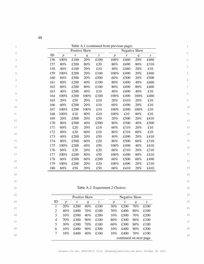
48

1 1

2 2

3 3

4 4

5 5

6 6

7 7

8 8

9 9

10 10

11 11

12 12

13 13

14 14

15 15

16 16

17 17

18 18

19 19

20 20

21 21

22 22

23 23

24 24

25 25

26 26

27 27

28 28

29 29


ID p x q y p x q y156 100% £100 20% £100 100% £460 20% £460157 80% £200 80% £20 80% £490 80% £310158 40% £100 20% £10 40% £460 20% £10159 100% £200 20% £100 100% £490 20% £460160 60% £500 20% £500 60% £500 20% £500161 80% £200 40% £100 80% £490 40% £460162 80% £200 80% £100 80% £490 80% £460163 40% £200 40% £10 40% £490 40% £10164 100% £200 100% £100 100% £490 100% £460165 20% £50 20% £10 20% £410 20% £10166 60% £200 20% £10 60% £490 20% £10167 100% £200 100% £10 100% £490 100% £10168 100% £10 80% £10 100% £10 80% £10169 20% £500 20% £50 20% £500 20% £410170 80% £500 40% £500 80% £500 40% £500171 60% £20 20% £10 60% £310 20% £10172 80% £20 60% £10 80% £310 60% £10173 40% £200 20% £50 40% £490 20% £410174 80% £500 60% £20 80% £500 60% £310175 100% £200 40% £50 100% £490 40% £410176 60% £20 20% £20 60% £310 20% £310177 100% £200 80% £50 100% £490 80% £410178 60% £500 60% £200 60% £500 60% £490179 100% £200 20% £20 100% £490 20% £310180 60% £50 20% £50 60% £410 20% £410


Positive Skew Negative SkewID p x q y p x q y1 20% £200 40% £100 30% £200 70% £1002 40% £400 70% £100 70% £400 80% £1003 10% £500 40% £200 10% £500 70% £2004 70% £300 90% £100 80% £300 90% £1005 30% £300 70% £100 60% £300 80% £1006 10% £400 90% £300 10% £400 90% £3007 10% £400 40% £100 10% £400 70% £100



49

1 1

2 2

3 3

4 4

5 5

6 6

7 7

8 8

9 9

10 10

11 11

12 12

13 13

14 14

15 15

16 16

17 17

18 18

19 19

20 20

21 21

22 22

23 23

24 24

25 25

26 26

27 27

28 28

29 29


ID p x q y p x q y8 30% £400 40% £300 60% £400 70% £3009 10% £400 20% £100 10% £400 30% £10010 20% £500 70% £400 30% £500 80% £40011 40% £500 70% £400 70% £500 80% £40012 30% £400 70% £300 60% £400 80% £30013 30% £300 40% £100 60% £300 70% £10014 20% £400 30% £200 30% £400 60% £20015 20% £500 30% £400 30% £500 60% £40016 10% £300 70% £200 10% £300 80% £20017 30% £400 70% £200 60% £400 80% £20018 10% £500 30% £200 10% £500 60% £20019 20% £400 40% £100 30% £400 70% £10020 20% £400 40% £200 30% £400 70% £20021 10% £300 40% £100 10% £300 70% £10022 10% £400 70% £300 10% £400 80% £30023 30% £500 70% £200 60% £500 80% £20024 40% £300 90% £100 70% £300 90% £10025 20% £500 90% £400 30% £500 90% £40026 10% £400 20% £200 10% £400 30% £20027 10% £300 70% £100 10% £300 80% £10028 40% £200 90% £100 70% £200 90% £10029 70% £400 90% £200 80% £400 90% £20030 10% £200 90% £100 10% £200 90% £10031 20% £400 70% £200 30% £400 80% £20032 20% £500 40% £100 30% £500 70% £10033 10% £500 20% £100 10% £500 30% £10034 70% £400 90% £100 80% £400 90% £10035 30% £500 90% £200 60% £500 90% £20036 40% £400 70% £300 70% £400 80% £30037 40% £400 90% £200 70% £400 90% £20038 20% £400 30% £300 30% £400 60% £30039 70% £200 90% £100 80% £200 90% £10040 30% £300 40% £200 60% £300 70% £20041 10% £500 70% £400 10% £500 80% £40042 10% £300 90% £100 10% £300 90% £10043 20% £300 90% £100 30% £300 90% £10044 20% £500 40% £400 30% £500 70% £40045 40% £400 90% £100 70% £400 90% £10046 40% £300 70% £200 70% £300 80% £200



50

1 1

2 2

3 3

4 4

5 5

6 6

7 7

8 8

9 9

10 10

11 11

12 12

13 13

14 14

15 15

16 16

17 17

18 18

19 19

20 20

21 21

22 22

23 23

24 24

25 25

26 26

27 27

28 28

29 29


ID p x q y p x q y47 20% £500 70% £200 30% £500 80% £20048 30% £200 90% £100 60% £200 90% £10049 30% £300 70% £200 60% £300 80% £20050 10% £500 70% £300 10% £500 80% £30051 20% £400 90% £200 30% £400 90% £20052 40% £500 70% £300 70% £500 80% £30053 30% £500 70% £300 60% £500 80% £30054 10% £500 90% £300 10% £500 90% £30055 30% £200 70% £100 60% £200 80% £10056 20% £500 90% £200 30% £500 90% £20057 10% £400 30% £200 10% £400 60% £20058 40% £500 90% £300 70% £500 90% £30059 10% £500 90% £100 10% £500 90% £10060 20% £200 90% £100 30% £200 90% £10061 40% £500 70% £200 70% £500 80% £20062 40% £500 90% £400 70% £500 90% £40063 40% £300 70% £100 70% £300 80% £10064 10% £200 20% £100 10% £200 30% £10065 20% £300 90% £200 30% £300 90% £20066 10% £200 40% £100 10% £200 70% £10067 10% £500 90% £200 10% £500 90% £20068 20% £500 70% £100 30% £500 80% £10069 20% £400 70% £100 30% £400 80% £10070 30% £500 90% £100 60% £500 90% £10071 40% £400 70% £200 70% £400 80% £20072 20% £500 90% £300 30% £500 90% £30073 30% £400 40% £200 60% £400 70% £20074 30% £500 40% £100 60% £500 70% £10075 30% £400 70% £100 60% £400 80% £10076 20% £500 30% £200 30% £500 60% £20077 40% £200 70% £100 70% £200 80% £10078 10% £300 90% £200 10% £300 90% £20079 10% £300 30% £100 10% £300 60% £10080 10% £300 30% £200 10% £300 60% £20081 10% £400 40% £200 10% £400 70% £20082 30% £300 90% £100 60% £300 90% £10083 20% £500 40% £300 30% £500 70% £30084 30% £400 90% £100 60% £400 90% £10085 10% £500 70% £100 10% £500 80% £100



51

1 1

2 2

3 3

4 4

5 5

6 6

7 7

8 8

9 9

10 10

11 11

12 12

13 13

14 14

15 15

16 16

17 17

18 18

19 19

20 20

21 21

22 22

23 23

24 24

25 25

26 26

27 27

28 28

29 29


ID p x q y p x q y86 40% £400 90% £300 70% £400 90% £30087 30% £300 90% £200 60% £300 90% £20088 20% £500 90% £100 30% £500 90% £10089 20% £400 30% £100 30% £400 60% £10090 30% £400 90% £200 60% £400 90% £20091 20% £400 40% £300 30% £400 70% £30092 20% £400 90% £300 30% £400 90% £30093 20% £400 70% £300 30% £400 80% £30094 30% £500 90% £400 60% £500 90% £40095 70% £300 90% £200 80% £300 90% £20096 20% £500 40% £200 30% £500 70% £20097 20% £300 40% £100 30% £300 70% £10098 20% £300 40% £200 30% £300 70% £20099 70% £500 90% £400 80% £500 90% £400100 10% £500 20% £400 10% £500 30% £400101 10% £400 90% £200 10% £400 90% £200102 30% £500 40% £400 60% £500 70% £400103 10% £500 40% £400 10% £500 70% £400104 70% £500 90% £300 80% £500 90% £300105 10% £500 90% £400 10% £500 90% £400106 30% £500 40% £300 60% £500 70% £300107 70% £500 90% £100 80% £500 90% £100108 70% £500 90% £200 80% £500 90% £200109 20% £300 70% £100 30% £300 80% £100110 10% £300 20% £100 10% £300 30% £100111 10% £500 40% £100 10% £500 70% £100112 10% £200 30% £100 10% £200 60% £100113 10% £300 20% £200 10% £300 30% £200114 10% £500 70% £200 10% £500 80% £200115 20% £400 90% £100 30% £400 90% £100116 10% £400 70% £100 10% £400 80% £100117 20% £300 30% £200 30% £300 60% £200118 30% £500 40% £200 60% £500 70% £200119 10% £500 40% £300 10% £500 70% £300120 40% £500 90% £100 70% £500 90% £100121 20% £500 10% £400 30% £500 10% £400122 90% £200 70% £200 90% £200 80% £200123 70% £500 10% £300 80% £500 10% £300124 40% £400 30% £300 70% £400 60% £300



52

1 1

2 2

3 3

4 4

5 5

6 6

7 7

8 8

9 9

10 10

11 11

12 12

13 13

14 14

15 15

16 16

17 17

18 18

19 19

20 20

21 21

22 22

23 23

24 24

25 25

26 26

27 27

28 28

29 29


ID p x q y p x q y125 40% £500 30% £200 70% £500 60% £200126 90% £300 90% £200 90% £300 90% £200127 90% £400 20% £300 90% £400 30% £300128 90% £500 30% £300 90% £500 60% £300129 90% £500 70% £400 90% £500 80% £400130 90% £300 70% £100 90% £300 80% £100131 10% £400 10% £200 10% £400 10% £200132 30% £500 20% £100 60% £500 30% £100133 30% £500 30% £400 60% £500 60% £400134 20% £100 10% £100 30% £100 10% £100135 30% £500 10% £400 60% £500 10% £400136 20% £200 10% £200 30% £200 10% £200137 20% £400 10% £200 30% £400 10% £200138 40% £400 10% £300 70% £400 10% £300139 70% £200 30% £100 80% £200 60% £100140 30% £500 20% £300 60% £500 30% £300141 90% £500 30% £500 90% £500 60% £500142 70% £300 70% £200 80% £300 80% £200143 40% £300 20% £200 70% £300 30% £200144 30% £300 20% £100 60% £300 30% £100145 90% £500 40% £100 90% £500 70% £100146 90% £400 70% £200 90% £400 80% £200147 90% £500 10% £400 90% £500 10% £400148 70% £400 40% £200 80% £400 70% £200149 70% £300 10% £200 80% £300 10% £200150 90% £500 90% £100 90% £500 90% £100


Positive Skew Negative SkewID x1 t1 x2 t2 x1 t1 x2 t21 £500 2 months £20 2 days £500 2 months £310 2 days2 £500 1 month £50 2 weeks £500 1 month £410 2 weeks3 £500 2 months £50 1 day £500 2 months £410 1 day4 £200 1 year £10 2 weeks £490 1 year £10 2 weeks5 £50 6 months £20 2 weeks £410 6 months £310 2 weeks6 £100 2 months £50 1 day £460 2 months £410 1 day



53

1 1

2 2

3 3

4 4

5 5

6 6

7 7

8 8

9 9

10 10

11 11

12 12

13 13

14 14

15 15

16 16

17 17

18 18

19 19

20 20

21 21

22 22

23 23

24 24

25 25

26 26

27 27

28 28

29 29


ID x1 t1 x2 t2 x1 t1 x2 t27 £100 6 months £10 1 week £460 6 months £10 1 week8 £500 1 month £200 1 day £500 1 month £490 1 day9 £500 6 months £10 2 weeks £500 6 months £10 2 weeks10 £500 2 months £200 2 weeks £500 2 months £490 2 weeks11 £500 2 months £20 1 week £500 2 months £310 1 week12 £100 1 year £10 2 weeks £460 1 year £10 2 weeks13 £50 2 months £10 2 days £410 2 months £10 2 days14 £200 6 months £100 2 months £490 6 months £460 2 months15 £20 6 months £10 2 months £310 6 months £10 2 months16 £200 2 weeks £100 1 day £490 2 weeks £460 1 day17 £200 1 month £10 1 week £490 1 month £10 1 week18 £500 2 months £50 1 month £500 2 months £410 1 month19 £200 2 months £10 2 days £490 2 months £10 2 days20 £200 2 months £20 2 weeks £490 2 months £310 2 weeks21 £500 1 week £200 2 days £500 1 week £490 2 days22 £500 1 month £20 1 day £500 1 month £310 1 day23 £100 6 months £10 1 month £460 6 months £10 1 month24 £200 2 weeks £50 1 week £490 2 weeks £410 1 week25 £200 2 days £10 1 day £490 2 days £10 1 day26 £500 2 months £200 1 day £500 2 months £490 1 day27 £20 1 month £10 1 week £310 1 month £10 1 week28 £100 6 months £10 2 months £460 6 months £10 2 months29 £100 2 days £50 1 day £460 2 days £410 1 day30 £50 2 months £20 2 weeks £410 2 months £310 2 weeks31 £100 2 weeks £20 2 days £460 2 weeks £310 2 days32 £200 2 months £100 1 month £490 2 months £460 1 month33 £500 6 months £20 2 months £500 6 months £310 2 months34 £200 2 months £50 1 day £490 2 months £410 1 day35 £50 6 months £20 1 day £410 6 months £310 1 day36 £500 1 month £100 2 days £500 1 month £460 2 days37 £100 1 year £20 1 week £460 1 year £310 1 week38 £500 6 months £200 2 weeks £500 6 months £490 2 weeks39 £500 6 months £50 2 weeks £500 6 months £410 2 weeks40 £200 1 month £10 2 weeks £490 1 month £10 2 weeks41 £500 1 year £10 2 months £500 1 year £10 2 months42 £20 2 months £10 1 month £310 2 months £10 1 month43 £20 2 months £10 2 weeks £310 2 months £10 2 weeks44 £500 6 months £200 2 months £500 6 months £490 2 months45 £200 1 year £10 1 month £490 1 year £10 1 month



54

1 1

2 2

3 3

4 4

5 5

6 6

7 7

8 8

9 9

10 10

11 11

12 12

13 13

14 14

15 15

16 16

17 17

18 18

19 19

20 20

21 21

22 22

23 23

24 24

25 25

26 26

27 27

28 28

29 29


ID x1 t1 x2 t2 x1 t1 x2 t246 £500 1 year £20 1 week £500 1 year £310 1 week47 £200 6 months £100 2 days £490 6 months £460 2 days48 £200 2 months £10 1 day £490 2 months £10 1 day49 £100 2 weeks £50 2 days £460 2 weeks £410 2 days50 £200 6 months £100 1 day £490 6 months £460 1 day51 £20 1 month £10 2 days £310 1 month £10 2 days52 £100 2 weeks £20 1 week £460 2 weeks £310 1 week53 £200 1 month £100 1 day £490 1 month £460 1 day54 £100 6 months £20 1 month £460 6 months £310 1 month55 £200 2 days £50 1 day £490 2 days £410 1 day56 £500 6 months £50 2 days £500 6 months £410 2 days57 £50 1 year £20 2 weeks £410 1 year £310 2 weeks58 £20 1 year £10 2 days £310 1 year £10 2 days59 £200 2 weeks £50 1 day £490 2 weeks £410 1 day60 £500 1 year £100 1 week £500 1 year £460 1 week61 £500 2 months £10 1 day £500 2 months £10 1 day62 £20 1 year £10 1 month £310 1 year £10 1 month63 £200 2 months £50 2 weeks £490 2 months £410 2 weeks64 £100 1 year £10 2 days £460 1 year £10 2 days65 £200 6 months £50 1 week £490 6 months £410 1 week66 £100 1 year £20 1 day £460 1 year £310 1 day67 £500 2 weeks £50 2 days £500 2 weeks £410 2 days68 £200 1 month £20 1 week £490 1 month £310 1 week69 £50 2 days £10 1 day £410 2 days £10 1 day70 £100 2 weeks £50 1 week £460 2 weeks £410 1 week71 £500 6 months £10 1 day £500 6 months £10 1 day72 £50 6 months £10 2 months £410 6 months £10 2 months73 £500 1 year £20 1 month £500 1 year £310 1 month74 £50 1 month £20 2 weeks £410 1 month £310 2 weeks75 £200 2 weeks £50 2 days £490 2 weeks £410 2 days76 £200 1 week £100 1 day £490 1 week £460 1 day77 £500 6 months £100 2 months £500 6 months £460 2 months78 £500 1 week £50 1 day £500 1 week £410 1 day79 £500 6 months £50 1 day £500 6 months £410 1 day80 £500 2 weeks £200 1 week £500 2 weeks £490 1 week81 £200 6 months £50 2 weeks £490 6 months £410 2 weeks82 £200 1 week £10 1 day £490 1 week £10 1 day83 £100 2 months £10 1 week £460 2 months £10 1 week84 £50 1 week £20 2 days £410 1 week £310 2 days



55

1 1

2 2

3 3

4 4

5 5

6 6

7 7

8 8

9 9

10 10

11 11

12 12

13 13

14 14

15 15

16 16

17 17

18 18

19 19

20 20

21 21

22 22

23 23

24 24

25 25

26 26

27 27

28 28

29 29


ID x1 t1 x2 t2 x1 t1 x2 t285 £100 6 months £10 1 day £460 6 months £10 1 day86 £50 1 week £10 1 day £410 1 week £10 1 day87 £500 2 weeks £50 1 week £500 2 weeks £410 1 week88 £20 6 months £10 1 day £310 6 months £10 1 day89 £500 1 week £100 2 days £500 1 week £460 2 days90 £100 1 year £50 6 months £460 1 year £410 6 months91 £20 2 weeks £10 1 day £310 2 weeks £10 1 day92 £200 2 months £100 2 weeks £490 2 months £460 2 weeks93 £20 1 year £10 2 weeks £310 1 year £10 2 weeks94 £100 1 year £50 1 week £460 1 year £410 1 week95 £100 1 year £10 1 week £460 1 year £10 1 week96 £500 2 weeks £100 2 days £500 2 weeks £460 2 days97 £500 2 months £100 2 days £500 2 months £460 2 days98 £100 2 months £20 2 days £460 2 months £310 2 days99 £100 1 week £10 1 day £460 1 week £10 1 day100 £500 6 months £100 1 week £500 6 months £460 1 week101 £50 1 year £10 1 week £410 1 year £10 1 week102 £500 1 month £200 2 days £500 1 month £490 2 days103 £50 2 months £10 2 weeks £410 2 months £10 2 weeks104 £500 1 year £50 1 day £500 1 year £410 1 day105 £50 1 year £20 6 months £410 1 year £310 6 months106 £200 1 week £20 2 days £490 1 week £310 2 days107 £500 1 year £200 1 day £500 1 year £490 1 day108 £500 6 months £100 1 month £500 6 months £460 1 month109 £200 1 year £100 2 weeks £490 1 year £460 2 weeks110 £500 2 months £200 1 month £500 2 months £490 1 month111 £200 6 months £50 1 month £490 6 months £410 1 month112 £500 6 months £200 1 week £500 6 months £490 1 week113 £100 2 months £10 2 weeks £460 2 months £10 2 weeks114 £200 1 month £50 2 weeks £490 1 month £410 2 weeks115 £500 1 week £10 1 day £500 1 week £10 1 day116 £500 1 year £100 6 months £500 1 year £460 6 months117 £200 2 months £10 1 month £490 2 months £10 1 month118 £500 2 months £10 1 month £500 2 months £10 1 month119 £500 2 months £200 1 week £500 2 months £490 1 week120 £50 6 months £20 1 week £410 6 months £310 1 week121 £200 1 month £200 2 weeks £490 1 month £490 2 weeks122 £50 1 month £20 2 months £410 1 month £310 2 months123 £100 2 days £10 2 weeks £460 2 days £10 2 weeks



56

1 1

2 2

3 3

4 4

5 5

6 6

7 7

8 8

9 9

10 10

11 11

12 12

13 13

14 14

15 15

16 16

17 17

18 18

19 19

20 20

21 21

22 22

23 23

24 24

25 25

26 26

27 27

28 28

29 29


ID x1 t1 x2 t2 x1 t1 x2 t2124 £100 6 months £10 1 year £460 6 months £10 1 year125 £500 1 day £200 1 week £500 1 day £490 1 week126 £500 2 months £100 1 year £500 2 months £460 1 year127 £500 2 days £10 1 week £500 2 days £10 1 week128 £500 1 year £500 1 month £500 1 year £500 1 month129 £20 2 days £20 1 day £310 2 days £310 1 day130 £100 2 months £10 6 months £460 2 months £10 6 months131 £200 1 day £20 2 weeks £490 1 day £310 2 weeks132 £10 6 months £10 2 months £10 6 months £10 2 months133 £20 1 year £20 1 month £310 1 year £310 1 month134 £500 1 week £200 2 weeks £500 1 week £490 2 weeks135 £10 2 months £10 1 month £10 2 months £10 1 month136 £100 2 weeks £20 2 weeks £460 2 weeks £310 2 weeks137 £200 1 week £10 6 months £490 1 week £10 6 months138 £500 2 days £200 6 months £500 2 days £490 6 months139 £100 1 day £10 1 week £460 1 day £10 1 week140 £200 6 months £200 2 days £490 6 months £490 2 days141 £50 2 months £50 2 days £410 2 months £410 2 days142 £50 6 months £10 6 months £410 6 months £10 6 months143 £100 1 week £50 1 week £460 1 week £410 1 week144 £10 6 months £10 1 week £10 6 months £10 1 week145 £200 1 week £50 1 year £490 1 week £410 1 year146 £200 1 month £10 2 months £490 1 month £10 2 months147 £500 6 months £500 2 months £500 6 months £500 2 months148 £500 6 months £200 1 year £500 6 months £490 1 year149 £500 2 days £200 1 year £500 2 days £490 1 year150 £20 1 day £10 1 week £310 1 day £10 1 week


Positive Skew Negative SkewID x1 t1 x2 t2 x1 t1 x2 t21 £200 1 year £100 6 months £400 10 months £200 2 months2 £500 6 months £300 1 week £200 1 year £100 8 months3 £400 6 months £300 1 month £300 10 months £200 8 months4 £300 2 weeks £200 1 week £300 2 months £200 1 day5 £300 1 year £200 1 day £500 4 months £300 2 months



57

1 1

2 2

3 3

4 4

5 5

6 6

7 7

8 8

9 9

10 10

11 11

12 12

13 13

14 14

15 15

16 16

17 17

18 18

19 19

20 20

21 21

22 22

23 23

24 24

25 25

26 26

27 27

28 28

29 29

Table A.4 (continued from previous page)Positive Skew Uniform

ID x1 t1 x2 t2 x1 t1 x2 t26 £500 2 months £100 2 days £300 4 months £100 2 months7 £500 1 month £400 2 weeks £200 2 months £100 1 day8 £300 6 months £200 1 day £500 6 months £100 4 months9 £300 2 weeks £100 1 week £400 1 year £300 1 day10 £400 2 months £100 1 month £300 6 months £100 2 months11 £500 2 months £200 2 weeks £300 4 months £100 1 day12 £500 1 year £400 1 month £500 8 months £200 6 months13 £500 2 weeks £300 2 days £500 8 months £200 2 months14 £400 1 year £100 2 days £500 1 year £300 1 day15 £500 2 months £100 1 week £400 6 months £300 2 months16 £500 1 year £200 2 days £500 1 year £100 10 months17 £400 2 weeks £100 1 day £500 1 year £300 6 months18 £300 6 months £100 2 months £500 10 months £100 6 months19 £500 2 weeks £400 1 day £500 8 months £300 4 months20 £500 6 months £400 2 days £300 10 months £100 6 months21 £400 2 months £300 2 weeks £300 8 months £200 2 months22 £500 2 weeks £300 1 week £400 1 year £300 6 months23 £500 6 months £400 2 months £500 4 months £100 1 day24 £500 1 week £100 1 day £300 1 year £100 10 months25 £400 2 months £100 1 day £400 10 months £200 4 months26 £400 1 month £300 2 weeks £400 1 year £300 8 months27 £500 2 months £300 1 week £500 10 months £300 6 months28 £400 1 month £200 1 week £400 8 months £100 6 months29 £200 6 months £100 1 week £500 4 months £100 2 months30 £200 2 weeks £100 1 week £300 1 year £200 8 months31 £500 1 week £300 1 day £400 8 months £300 4 months32 £500 6 months £100 1 month £400 10 months £300 4 months33 £300 2 weeks £200 2 days £500 8 months £300 6 months34 £400 6 months £100 1 month £200 6 months £100 4 months35 £500 1 year £200 1 day £300 4 months £200 1 day36 £400 1 year £300 2 days £400 1 year £100 1 day37 £300 1 year £100 1 week £200 8 months £100 1 day38 £300 6 months £100 2 weeks £400 6 months £300 1 day39 £400 2 weeks £300 1 week £500 1 year £200 8 months40 £500 2 months £300 1 day £400 2 months £200 1 day41 £500 2 months £100 1 month £300 10 months £100 1 day42 £500 1 year £200 2 months £500 1 year £300 8 months43 £400 1 month £200 1 day £400 8 months £200 6 months44 £500 1 year £200 6 months £500 10 months £400 6 months



58

1 1

2 2

3 3

4 4

5 5

6 6

7 7

8 8

9 9

10 10

11 11

12 12

13 13

14 14

15 15

16 16

17 17

18 18

19 19

20 20

21 21

22 22

23 23

24 24

25 25

26 26

27 27

28 28

29 29


ID x1 t1 x2 t2 x1 t1 x2 t245 £400 1 year £300 2 weeks £200 10 months £100 1 day46 £400 2 months £200 1 day £400 10 months £200 6 months47 £300 2 months £100 2 weeks £500 4 months £300 1 day48 £400 2 months £300 2 days £500 8 months £400 6 months49 £500 2 days £400 1 day £400 6 months £100 4 months50 £300 1 month £200 2 days £400 4 months £200 1 day51 £500 1 month £400 2 days £400 1 year £100 2 months52 £400 1 year £200 1 day £500 1 year £100 4 months53 £500 2 weeks £200 2 days £200 10 months £100 8 months54 £400 1 month £100 1 week £200 8 months £100 4 months55 £200 2 weeks £100 2 days £500 8 months £100 2 months56 £500 1 year £300 1 week £500 10 months £100 2 months57 £400 2 days £300 1 day £400 8 months £200 1 day58 £400 1 month £100 1 day £400 1 year £100 6 months59 £300 1 month £200 1 week £400 8 months £100 4 months60 £500 1 month £300 1 week £500 10 months £400 4 months61 £200 2 months £100 2 weeks £400 10 months £300 8 months62 £400 2 months £300 1 day £400 1 year £200 8 months63 £400 1 month £300 2 days £200 4 months £100 1 day64 £400 6 months £300 1 week £400 10 months £300 2 months65 £200 2 weeks £100 1 day £500 10 months £300 1 day66 £300 1 month £100 2 weeks £500 6 months £200 4 months67 £300 1 week £100 1 day £400 2 months £300 1 day68 £500 2 months £200 1 month £400 10 months £100 2 months69 £500 2 weeks £200 1 day £500 6 months £100 2 months70 £400 1 year £100 2 weeks £400 8 months £300 2 months71 £200 1 week £100 2 days £300 6 months £100 4 months72 £400 2 weeks £200 2 days £200 4 months £100 2 months73 £500 6 months £300 1 day £500 6 months £300 1 day74 £200 2 months £100 1 week £500 8 months £300 2 months75 £400 1 week £200 1 day £400 6 months £100 2 months76 £300 1 year £200 2 weeks £400 4 months £300 1 day77 £500 1 month £200 2 days £500 10 months £200 6 months78 £200 1 year £100 1 week £500 8 months £200 1 day79 £300 2 weeks £100 1 day £400 8 months £200 4 months80 £400 1 year £200 6 months £500 2 months £300 1 day81 £400 2 months £100 2 weeks £500 8 months £200 4 months82 £400 1 year £300 1 week £200 8 months £100 6 months83 £400 2 months £300 1 week £500 1 year £200 2 months



59

1 1

2 2

3 3

4 4

5 5

6 6

7 7

8 8

9 9

10 10

11 11

12 12

13 13

14 14

15 15

16 16

17 17

18 18

19 19

20 20

21 21

22 22

23 23

24 24

25 25

26 26

27 27

28 28

29 29


ID x1 t1 x2 t2 x1 t1 x2 t284 £500 1 year £100 1 month £500 10 months £200 1 day85 £200 1 month £100 2 weeks £300 6 months £200 2 months86 £200 2 months £100 2 days £500 10 months £400 2 months87 £200 6 months £100 1 month £500 6 months £200 2 months88 £500 1 year £400 1 week £500 1 year £100 6 months89 £400 1 year £200 2 months £500 10 months £200 8 months90 £500 2 weeks £200 1 week £500 6 months £400 1 day91 £500 1 year £400 1 day £500 8 months £400 2 months92 £400 2 weeks £200 1 week £300 1 year £200 6 months93 £500 2 months £200 1 day £400 8 months £300 1 day94 £400 2 weeks £300 2 days £500 10 months £100 4 months95 £400 6 months £300 2 months £400 8 months £100 1 day96 £300 1 year £200 1 week £400 1 year £300 4 months97 £300 6 months £200 2 days £200 10 months £100 6 months98 £400 6 months £300 1 day £300 8 months £100 6 months99 £500 1 month £100 1 week £500 1 year £100 1 day100 £300 1 year £200 2 months £300 1 year £100 6 months101 £400 1 year £100 1 month £500 1 year £400 8 months102 £300 1 month £100 1 day £400 6 months £300 4 months103 £500 1 month £300 1 day £400 8 months £300 6 months104 £400 6 months £200 1 month £500 8 months £400 4 months105 £200 6 months £100 2 months £300 10 months £200 1 day106 £400 1 week £300 1 day £400 10 months £100 1 day107 £300 1 month £200 1 day £500 10 months £400 8 months108 £400 1 year £100 1 week £300 1 year £200 2 months109 £500 1 year £200 1 week £500 1 year £200 4 months110 £400 6 months £300 2 days £400 1 year £200 4 months111 £500 1 year £300 6 months £500 2 months £400 1 day112 £400 6 months £100 2 months £500 6 months £300 4 months113 £500 6 months £200 2 days £300 4 months £200 2 months114 £400 2 months £100 2 days £200 6 months £100 2 months115 £500 2 days £100 1 day £500 1 year £300 10 months116 £200 1 year £100 2 months £300 8 months £100 4 months117 £500 1 month £100 1 day £300 8 months £100 2 months118 £500 6 months £200 2 weeks £400 10 months £200 1 day119 £200 2 days £100 1 day £500 1 year £200 10 months120 £300 2 months £100 1 week £400 6 months £200 1 day121 £400 2 weeks £100 1 month £400 8 months £300 10 months122 £200 2 weeks £100 6 months £400 8 months £200 8 months



60

1 1

2 2

3 3

4 4

5 5

6 6

7 7

8 8

9 9

10 10

11 11

12 12

13 13

14 14

15 15

16 16

17 17

18 18

19 19

20 20

21 21

22 22

23 23

24 24

25 25

26 26

27 27

28 28

29 29


ID x1 t1 x2 t2 x1 t1 x2 t2123 £500 1 day £300 2 months £400 2 months £200 6 months124 £300 1 day £200 6 months £500 1 day £400 6 months125 £100 2 weeks £100 6 months £400 1 day £100 1 day126 £400 2 days £400 6 months £100 1 day £100 8 months127 £500 1 day £300 6 months £500 6 months £300 10 months128 £500 2 weeks £200 1 year £400 1 day £100 1 year129 £200 1 week £100 1 week £500 8 months £300 10 months130 £300 1 week £100 6 months £500 1 day £400 1 day131 £300 1 day £300 2 days £500 2 months £300 4 months132 £500 2 days £400 6 months £200 4 months £100 10 months133 £300 1 day £100 2 weeks £500 1 day £200 4 months134 £400 2 days £300 1 month £100 2 months £100 4 months135 £400 2 weeks £300 1 month £500 4 months £100 6 months136 £400 1 day £200 2 days £400 2 months £400 4 months137 £200 1 day £200 2 weeks £100 1 day £100 1 year138 £400 1 week £300 2 weeks £300 6 months £200 8 months139 £500 2 days £500 6 months £300 2 months £200 2 months140 £200 2 months £200 1 year £500 10 months £300 1 year141 £500 2 days £100 1 week £500 10 months £100 1 year142 £200 1 day £100 1 day £300 1 day £200 6 months143 £500 2 weeks £400 2 months £300 4 months £200 8 months144 £500 1 year £200 1 year £500 8 months £200 1 year145 £200 2 weeks £100 2 weeks £300 1 day £300 4 months146 £200 1 day £100 2 weeks £200 2 months £200 10 months147 £500 2 days £500 1 year £500 4 months £300 1 year148 £300 2 weeks £100 6 months £500 1 day £500 2 months149 £300 1 week £200 6 months £400 10 months £300 10 months150 £500 2 months £200 1 year £500 4 months £400 4 months

REFERENCES

ABDELLAOUI, M. (2000): “Parameter free elicitation of utilities and probability weighting func-tions,” Management Science, 46, 1497–1512.

AINSLIE, G. (1975): “Specious reward: A behavioural theory of impulsiveness and impulsecontrol,” Psychological Bulletin, 82, 463–496.

ALLAIS, M. (1953): “Le comportement de l’homme rationel devant le risque: Critique des pos-tulats et axioms de l’ecole americaine [Rational man’s behavior in face of risk: Critique of theAmerican School’s postulates and axioms],” Econometrica, 21, 503–546.

ARIELY, D., B. KOSZEGI, N. MAZAR, AND K. SHAMPAN’ER (2008): “Price-sensitive prefer-ences,” .


61

1 1

2 2

3 3

4 4

5 5

6 6

7 7

8 8

9 9

10 10

11 11

12 12

13 13

14 14

15 15

16 16

17 17

18 18

19 19

20 20

21 21

22 22

23 23

24 24

25 25

26 26

27 27

28 28

29 29

BECKER, G. M., M. H. DEGROOT, AND J. MARSCHAK (1963): “Stochastic models of choicebehavior,” Behavioral Science, 8, 41–55.

(1964): “Measuring utility by a single-response sequential method,” Behavioral Science,9, 226–232.

BELL, D. E. (1985): “Disappointment in decision making under uncertainty,” Operations Re-search, 33, 1–27.

BENARTZI, S., AND R. H. THALER (2001): “Naive diversification strategies in defined contri-bution saving plans,” American Economic Review, 91, 79–98.

BENTHAM, J. (1970): An introduction to the principles of morals and legislation. Athlone, Lon-don.

BIRNBAUM, M. H. (1992): “Violations of the monotonicity and contextual effects in choice-based certainty equivalents,” Psychological Science, 3, 310–314.

(2008): “New paradoxes of risky decision making,” Psychological Review, 115, 453–501.

BIRNBAUM, M. H., AND A. CHAVEZ (1997): “Tests of theories of decision making: Violationsof branch independence and distribution independence,” Organizational Behavior and HumanDecision Processes, 71, 161–194.

BLAVATSKYY, P. R. (2007): “Stochastic expected utility theory,” Journal of Risk and Uncer-tainty, 34, 259–286.

BLAVATSKYY, P. R., AND G. POGREBNA (2010): “Models of stochastic choice and decisiontheories: Why both are important for analyzing decisions,” Journal of Applied Econometrics,25, 963–986.

BLEICHRODT, H., AND J. L. PINTO (2000): “A parameter-free elicitation of the probabilityweighting function in medical decision analysis,” Management Science, 46, 1485–1496.

BOYCE, C. J. (2009): “Subjective well-being: An intersection between economics and psychol-ogy,” Ph.D. thesis, Warwick University, Coventry, England.

BRANDSTATTER, E., G. GIGERENZER, AND R. HERTWIG (2006): “The priority heuristic:Making choices without trade-offs,” Psychological Review, 113, 409–432.

BROWN, G. D. A., J. GARDNER, A. J. OSWALD, AND J. QIAN (2008): “Does wage rank affectemployees’ well-being?,” Industrial Relations, 47, 355–389.

BUSEMEYER, J. R. (1985): “Decision making under uncertainty: A comparison of simple scal-ability, fixed sample, and sequential sampling models,” Journal of Experimental Psychology,11, 538564.

BUSEMEYER, J. R., AND J. T. TOWNSEND (1993): “Decision field theory: A dynamic-cognitive approach to decision making in an uncertain environment,” Psychological Review,100, 432–459.

CAMERER, C. F. (1995): “Individual decision making,” in Handbook of experimental eco-nomics, ed. by J. Kagel, and A. E. Roth, pp. 587–703. Princeton University Press, Princeton,NJ.

DORLET, A., I. SIMONSON, AND A. TVERSKY (2000): “Indifference curves that travel withthe choice set,” Marketing Letters, 11, 199–209.

EDWARDS, W. (1962): “Subjective probabilities inferred from decisions,” Psychological Review,69, 109–135.

EREV, I., A. E. ROTH, R. L. SLONIM, AND G. BARRON (2002): “Combining a theoreticalprediction with experimental evidence,” .

GONZALEZ, R., AND G. WU (1999): “On the shape of the probability weighting function,”Cognitive Psychology, 38, 129–166.

GUL, F. (1991): “A theory of disappointment aversion,” Econometrica, 59, 667–686.KAHNEMAN, D., J. L. KNETSCH, AND R. H. THALER (1991): “Anomalies: The endowment


62

1 1

2 2

3 3

4 4

5 5

6 6

7 7

8 8

9 9

10 10

11 11

12 12

13 13

14 14

15 15

16 16

17 17

18 18

19 19

20 20

21 21

22 22

23 23

24 24

25 25

26 26

27 27

28 28

29 29

effect, loss aversion, and status quo bias,” Journal of Economic Perspectives, 5, 193–206.KAHNEMAN, D., AND A. TVERSKY (1979): “Prospect theory: An analysis of decision under

risk,” Econometrica, 47, 263–291.KORNIENKO, T. (2011): “A cognitive basis for context-dependent utility,” .KOSZEGI, B., AND M. RABIN (2006): “A model of reference-dependent preferences,” Quar-

terly Journal of Economics, 121, 1133–1165.(2007): “Reference-dependent risk attitudes,” American Economic Review, 97, 1047–

1073.LAIBSON, D. (1997): “Golden eggs and hyperbolic discounting,” Quarterly Journal of Eco-

nomics, 112, 443–477.LOEWENSTEIN, G., AND D. PRELEC (1992): “Anomalies in intertemporal choice: Evidence

and an interpretation,” Quarterly Journal of Economics, 107, 573–597.LOOMES, G. (2005): “Modelling the stochastic component of behaviour in experiments: Some

issues for the interpretation of data,” Experimental Economics, 8, 301–323.(2010): “Modeling choice and valuation in decision experiments,” Psychological Re-

view, 117, 902–924.LOOMES, G., AND R. SUGDEN (1982): “Regret theory: An alternative theory of rational choice

under uncertainty,” Economic Journal, 92, 805–824.(1986): “Disappointment and dynamic consistency in choice under uncertainty,” Review

of Economic Studies, 53, 271–282.LUCE, R. D. (1959): Individual choice behavior. Wiley, New York.LUCE, R. D. (2000): Utility of gains and losses: Measurement-theoretical and experimental

approaches. Erlbaum, Mahwah, NJ.MACCHERONI, F., M. MARINACCI, AND A. RUSTICHINI (2009a): “Pride and diversity in so-

cial economics,” .(2009b): “Social decision theory: Choosing within and between groups,” .

MAZUR, J. E. (1987): “An adjusting procedure for studying delayed reinforcement,” in Quanti-tative analyses of behavior: Vol. 5. The effect of delay and of intervening events on reinforce-ment value, ed. by M. L. Commons, J. E. Mazur, J. A. Nevin, and H. Rachlin, pp. 55–73.Erlbaum, Hillsdale, NJ.

PARDUCCI, A. (1965): “Category judgment: A range-frequency model,” Psychological Review,72, 407–418.

(1995): Happiness, pleasure and judgment: The contextual theory and its applications.Erlbaum, Mahwah, NJ.

PRELEC, D. (1998): “The probability weighting function,” Econometrica, 66, 497–527.QUIGGIN, J. (1993): Generalized expected utility theory: The rank-dependent model. Kluwer

Academic Publishers, Norwell, MA.RACHLIN, H., A. RAINERI, AND D. CROSS (1991): “Subjective probability and delay,” Journal

of the Experimental Analysis of Behavior, 55, 233–244.READ, D. (2001): “Is time-discounting hypoerbolic or subadditive?,” Journal of Risk and Un-

certainty, 23, 5–32.(2007): “Experienced utility: Utility theory from Jeremy Bentham to Daniel Kahneman,”

Thinking & Reasoning, 13, 45–61.SAMUELSON, P. A. (1937): “A note on measurement of utility,” Review of Economic Studies, 4,

155–161.SAVAGE, L. J. (1954): The foundations of statistics. Wiley, New York.SCHOEMAKER, P. J. H. (1982): “The expected utility model: Its variants, purposes, evidence,

and limitations,” Journal of Economic Literature, 20, 529–563.SCHOLTEN, M., AND D. READ (2010): “The psychology of intertemporal tradeoffs,” Psycho-


63

1 1

2 2

3 3

4 4

5 5

6 6

7 7

8 8

9 9

10 10

11 11

12 12

13 13

14 14

15 15

16 16

17 17

18 18

19 19

20 20

21 21

22 22

23 23

24 24

25 25

26 26

27 27

28 28

29 29

logical Review, 117, 925–944.SEYMOUR, B., AND S. M. MCCLURE (2008): “Anchors, scales and the relative coding of value

in the brain,” Current Opinion in Neurobiology, 18, 173–178.SHEPARD, R. N. (1957): “Stimulus and response generalization: A stochastic model relating

generalization to distance in psychological space,” Psychometrica, 22, 325–345.STARMER, C. (2000): “Developments in non-expected utility theory: The hunt for a descriptive

theory of choice under risk,” Journal of Economic Literature, 38, 332–382.STEWART, N. (2009): “Decision by sampling: The role of the decision environment in risky

choice,” Quarterly Journal of Experimental Psychology, 62, 1041–1062.STEWART, N., N. CHATER, AND G. D. A. BROWN (2006): “Decision by sampling,” Cognitive

Psychology, 53, 1–26.STEWART, N., N. CHATER, H. P. STOTT, AND S. REIMERS (2003): “Prospect relativity: How

choice options influence decision under risk,” Journal of Experimental Psychology: General,132, 23–46.

STEWART, N., AND K. SIMPSON (2008): “A decision-by-sampling account of decision underrisk,” in The probabilistic mind: Prospects for Bayesian cognitive science, ed. by N. Chater,and M. Oaksford, pp. 261–276. Oxford University Press, Oxford, England.

STIGLER, G. J. (1950a): “The development of utility theory. I,” Journal of Political Economy,58, 307–327.

(1950b): “The development of utility theory. II,” Journal of Political Economy, 58, 373–396.

THALER, R. H. (1981): “Some empirical evidence on dynamic inconsistency,” Economic Let-ters, 8, 201–207.

TOM, S. M., C. R. FOX, C. TREPEL, AND R. A. POLDRACK (2007): “The neural basis of lossaversion in decision-making under risk,” .

TREMBLAY, L., AND W. SCHULTZ (1999): “Relative reward preference in primate orbitofrontalcortex,” .

TVERSKY, A., AND D. KAHNEMAN (1992): “Advances in prospect theory: Cumulative repre-sentation of uncertainty,” Journal of Risk and Uncertainty, 5, 297–323.

UNGEMACH, C., N. STEWART, AND S. REIMERS (2011): “How incidental values from ourenvironment affect decisions about money, risk, and delay,” Psychological Science, 22, 253–260.

VON NEUMANN, M., AND O. MORGENSTERN (1947): Theory of games and economic behav-ior. Princeton University Press, Princeton, NJ, 2nd edn.

WU, G., AND R. GONZALEZ (1996): “Curvature of the probability weighting function,” Man-agement Science, 42, 1676–1690.

(1999): “Nonlinear decision weights in choice under uncertainty,” Management Science,45, 74–85.


on the origin of utility, weighting, and discounting

Documents