on the possibility of inflation targeting in kyrgyzstan the possibility of inflation targeting in...
TRANSCRIPT

GRADUATE SCHOOL OF DEVELOPMENT
Institute of Public Policy and Administration
On the Possibility of Inflation Targeting in Kyrgyzstan
Nurbek Jenish, Asel Kyrgyzbaeva
WORKING PAPER NO.8, 2012


On the Possibility of Inflation Targeting in Kyrgyzstan
Nurbek Jenish, Asel Kyrgyzbaeva
AbstractThe paper examines the possibility of adopting inflation targeting framework in Kyrgyzstan. The examination suggests that it is premature for Kyrgyzstan to adopt full-fledged IT framework since most of the prerequisites for the successful IT adoption are not in place. However, the analysis and the results of the DSGE model calibrated for the country suggest that the country may adopt some form of hybrid inflation targeting regime. More specifically, the economy could benefit from a more aggressive policy control of inflation and minor interventions on the foreign exchange markets.
Keywordsinflation targeting, monetary policy, Kyrgyzstan
JEL No: E52, E58.
INSTITUTE OF PUBLIC POLICY AND ADMINISTRATION
WORKING PAPER NO.8, 2012

On the Possibility of Inflation Targeting in Kyrgyzstan2
The Institute of Public Policy and Administration was established in 2011 to promote sys-tematic and in-depth research on issues related to the socio-economic development of Cen-tral Asia, and explore policy alternatives.
This paper is part of research being conducted for the “Regional Cooperation and Confidence Building in Central Asia and Afghanistan” (RCCB) project supported by the Government of Canada, Department of Foreign Affairs and International Trade.
The Institute of Public Policy and Administration is part of the Graduate School of Develop-ment, University of Central Asia. The University of Central Asia was founded in 2000. The Presidents of Kazakhstan, the Kyrgyz Republic, and Tajikistan, and His Highness the Aga Khan signed the International Treaty and Charter establishing this secular and private university, ratified by the respective parliaments, and registered with the United Nations. The Universi-ty is building simultaneously three fully-residential campuses in Tekeli (Kazakhstan), Naryn (Kyrgyz Republic) and Khorog (Tajikistan) that will open their doors to undergraduate and graduate students in 2016.
The Institute of Public Policy and Administration’s Working Papers is a peer-reviewed series that publishes original contributions on a broad range of topics dealing with social and eco-nomic issues, public administration and public policy as they relate to Central Asia.
About the authors
Nurbek Jenish is a research fellow at the IPPA and associate professor at the Department of Economics, American University of Central Asia. He holds PhD in economics from Central Eu-ropean University, and has an extensive experience in modeling and researching monetary and fiscal policy interactions in developing countries.
Asel Kyrgyzbaeva is an Assistant Professor at American University of Central Asia.
The authors would like to thank Oleksiy Kryvtsov and the participants of the December 2010 and July 2012 EERC Research Workshops for providing valuable comments. Financial sup-port from EERC, grant No R10-5151, is gratefully acknowledged.
Copyright © 2012University of Central Asia138 Toktogul Street, Bishkek 720001, Kyrgyz RepublicTel.: +996 (312) 910 822, E-mail: [email protected]
The findings, interpretations and conclusions expressed in this paper are entirely those of the author and do not necessary represent the view of the University of Central Asia
Text and data in this publication may be reproduced as long as the source is cited.

3Contents
Contents
Acronyms ................................................................................................................................................5
1. Introduction ...................................................................................................................................6
2. Literature Review .........................................................................................................................9
3. Economic performance and prerequisites for inflation targeting in Kyrgyzstan ........................................................................................................... 13
3.1 Overview of economic performance ........................................................................................13
3.2 Examination of IT prerequisites in Kyrgyzstan ...................................................................19
3.2.1. Central Bank independence and accountability and coordination between mon-etary and fiscal policies .................................................................................................................19
3.2.2. Vulnerability to external shocks and exchange rate pass-through .............................19
3.3.3. Financial sector development and stability ..........................................................................20
4. Small Open Economy Model ................................................................................................... 21
5. Results ........................................................................................................................................... 36
Sensitivity analysis .....................................................................................................................................45
6. Conclusions and policy implications................................................................................... 46
Annexes ............................................................................................................................................... 47

On the Possibility of Inflation Targeting in Kyrgyzstan4
Tables
Table 1. Growth rates of GDP and sectors ...........................................................................................14
Table 2. CPI composition and correlation between global food prices and inflation (2010) ..............................................................................................................................15
Table 3. Financial system health, as of end 2010 ..............................................................................20
Table 4. Model parameterization .............................................................................................................35
Table 5. Welfare maximizing monetary and fiscal policy parameter combinations..........37
Figures
Figure 1. Contributions to growth (supply) ..........................................................................................13
Figure 2. Remittances as a share of GDP ................................................................................................14
Figure 3. Consumer price inflation ...........................................................................................................16
Figure 4. Nominal exchange rate (end period) ....................................................................................16
Figure 5. Foreign currency denominated deposits and loans, % of total deposits and loans ...........................................................................................................................................17
Figure 6. Fiscal indicators, % of GDP .......................................................................................................18
Figure 7. Public external debt, % of GDP ................................................................................................18
Figure 8. Costs of managing exchange rate under consumption tax: Ωπ = 3, and Ω1 = 1.6 .....................................................................................................................38
Figure 9. Impulse responses to a negative 1 % shock to remittances under an optimized IT regime ...............................................................................................................39
Figure 10. Impulse responses to a negative 1 % shock to remittances under an optimized HIT regime .................................................................................................................42

5Acronyms
Acronyms
CB Central bank
C-CAPM Consumption capital asset pricing model
CIA Cash-in-advance
CPI Consumer price index
DSGE Dynamic stochastic general equilibrium
FDI Foreign direct investment
FFIT Full-fledged inflation targeting
FOCs First order conditions
HIT Hybrid inflation targeting
IMF International Monetary Fund
IT Inflation targeting
ITL Inflation targeting Lite
KR Kyrgyz Republic/Kyrgyzstan
NBKR National Bank of the Kyrgyz Republic
RF Russian Federation
WB World Bank

On the Possibility of Inflation Targeting in Kyrgyzstan6
1. Introduction
Since 1990, when New Zealand adopted an inflation targeting (IT) framework, IT has become a popular monetary policy strategy. As of 2010, 26 countries, half of them emerging market or low-income economies, were reported as IT countries.
Inflation targeting is a monetary policy framework under which a monetary authority publicly announces official quantitative targets or target ranges for the inflation rate over one or more time periods. The monetary authority also acknowledges explicitly that the monetary policy’s primary long-term goal is low and stable inflation. Four main elements of IT frameworks have been identified:1
1) An explicit central bank (CB) commitment to price stability as the primary objective of monetary policy, and a high degree of operational autonomy;
2) The public announcement of medium-term numerical targets for inflation;3) Accountability of the CB for attaining its inflation objectives; and4) Increased transparency of monetary policy strategy and implementation through
communication with the public and the markets about the plans and decisions of the CB.
What are the advantages of an IT monetary arrangement? Proponents of IT argue that it delivers a number of benefits relative to other operating strategies. First, the explicit commitment to long-term price stability and explicit communication of the inflation target rate to the public (and economic agents) help build credibility and anchor inflation expectations. Second, IT provides a considerable degree of flexibility for policy-makers. Central banks pursue inflation target over the medium- to long-term horizon, focusing on keeping inflation expectations at the target. This means that short-term deviations of inflation from the target are acceptable and do not necessarily undermine credibility. This leaves considerable scope for monetary authorities to respond to short-term phenomena, such as unemployment conditions and exchange rate fluctuations. Finally, in the case of monetary policy failures, IT entails lower economic costs compared to other monetary arrangements. For instance, in the case of failure of exchange rate pegs, which usually results in massive foreign exchange reserve losses, high inflation, financial and banking crises, and possibly debt defaults, the output (and fiscal) costs can be large. Under IT, the output costs of not meeting the inflation target are usually limited to higher inflation and a slower output growth as interest rates are increased to bring the inflation back to the target.
Arguments against IT can be summarized as follows. First, IT gets little support from the public which perceives the policy as having (literally) no goals other than to control inflation. Second, apart from inflation, governments and CBs do care about production, employment and exchange rates, and therefore focusing exclusively on hitting the inflation target can lead to poor economic outcomes, such as high exchange rate volatility and low growth. In the event of large supply-side shocks, such as sharp oil price increase, exclusive focus on pursuing
1 Frederic S. Mishkin, “Can Inflation Targeting Work in Emerging Market Countries?” National Bureau of Economic Research (NBER) Working Paper 10646, (Cambridge: NBER, July 2004); and Geoffrey Heenan, Marcel Peter, and Scott Roger, “Implementing Inflation Targeting: Institutional Arrangements, Target Design, and Communication,” International Monetary Fund Working Paper 06/278 (Washington DC: IMF, 2006).

71. Introduction
inflation target may lead to a highly unstable economy.2 In other words, IT provides too little discretion and therefore unnecessarily restrains growth. Third, in contrast to the second argument, some dispute that IT cannot help build credibility in countries that lack it. TheIT cannot anchor inflation expectations because it offers discretion as to when and how to bring inflation back to target, and because monetary authorities can change the target. Finally, IT can work only in countries that meet a set of institutional, technical, macroeconomic and financial preconditions.3
The importance of an appropriate institutional setting can be highlighted by the following fact. If a CB is not granted operational independence, its objectives may be dominated by fiscal considerations; the case of fiscal dominance. In such a case, if a fiscal authority follows an imprudent policy, the CB’s only objective becomes to adjust its monetary policy to ensure that government finances are sustainable in the medium to long-term.
Moreover, a number of macroeconomic and financial preconditions should be established before starting an IT regime. There should be sufficient stability in the external sector. If the economy is susceptible to frequent external disturbances, such as balance of payments and foreign exchange market shocks, monetary policy may face a tradeoff between reaching external stability and domestic objectives (low and stable inflation as specified by the IT framework). Furthermore, if the banking system is weak, an increase in the (short term) interest rate, which might be necessary to control inflation and is one of the main IT instruments, may lead to financial stress in the sector.
Given that most CBs in emerging economies lack credibility, and that these countries do not meet most of the required preconditions for IT adoption, critics of IT further argue that such economies are better off sticking to conventional monetary policy frameworks, such as exchange rate peg or money growth targeting regimes. Advocates of exchange rate peg argue that it entails lower transaction costs and exchange rate risk exposure. Money growth targeting is especially relevant for countries with underdeveloped financial sectors that do not allow them to hedge against long-term currency risks. Furthermore, countries with weak institutions can ‘import’ monetary credibility by pegging their currencies to a currency with a credible CB. However, exchange rate pegs have serious disadvantages. They constrain the ability of CBs to use monetary policy for short-term domestic stabilization; and in the world of perfect capital mobility, there is a possibility of a speculative attack on the pegged currency and ensuing currency crises.4
2 Benjamin Friedman and Kenneth Kuttner, “A Price Target for U.S. Monetary Policy? Lessons from the Experience with Money Growth Targets,” Brookings Papers on Economic Activity, no. 1, (Washington DC: The Brookings Institution,1996).
3 One of the preconditions for the successful adoption of IT is also a well-designed macro model of the economy. Please see Barry Eichengreen, Paul Masson, Miguel Savastano, and Sunil Sharma, “Transition Strategies and Nominal Anchors on the Road to Greater Exchange Rate Flexibility,” Essays in International Economics. (Princeton, N.J.: Princeton University, 1999) for a more detailed exposition of this point. Assessing the adequacy of the macro model employed by the National Bank of the Kyrgyz Republic and its technical and institutional abilities are beyond the scope of this study.
4 For a more detailed discussion of this point please see Maurice Obstfeld and Kenneth Rogoff, “The Mirage of Fixed Exchange Rates,” Journal of Economic Perspectives no. 9 vol. 4, (1995): 73-96.

On the Possibility of Inflation Targeting in Kyrgyzstan8
Exchange rate arrangements also have a bearing on aggregate demand through balance sheet effects on borrowing and investment expenditures. In most developing and emerging economies, external liabilities are denominated in foreign currencies. Exchange rate depreciation might reduce the net worth of domestic firms through increased expenditures on servicing of external debt and reduced revenues in terms of foreign currency.5 However, some studies suggest that, even in the presence of balance sheet effects, following a negative external shock, flexible exchange regime stabilizes economies better than a fixed exchange arrangement.6
In contrast to exchange rate pegging, monetary targeting (targeting monetary aggregates, for example, the monetary base, M1, M2 or M3) allows a greater freedom for a CB to adjust monetary policy to domestic conditions. Additionally, monetary aggregates can be measured accurately and without a long time lag. The monetary authority’s ability to control the rate of money growth is fairly good. Therefore, deviations of actual monetary growth rate from the rate can be quickly detected, and this can help build the credibility of CBs. However, monetary targeting becomes a less useful strategy if there is no reliable relationship between money growth and targeted macroeconomic variables, such as inflation and gross domestic product (GDP) growth rate.
Despite the arguments against IT, the number of emerging economies adopting IT in recent years has increased.7 Has the macroeconomic performance under IT been as good as, or better than, performance under alternative monetary regimes? Recent findings of a study of the macroeconomic performance of developed and emerging economies of 26 countries, before and after the adoption of IT, suggest that both IT and non-IT low-income countries experienced large reductions in the volatility of inflation and output, with the targeters registering larger declines in inflation volatility.8 High-income economies generally showed little changes in performance, before and after adopting IT. However, adoption of IT might not fully explain the relative improvement in performance, since many countries adopting IT also carried out broader structural and policy reforms.
The purpose of this paper is to contribute to growing literature on IT in emerging economies by examining the possibility of adopting lighter versions of the IT framework in Kyrgyzstan
5 Domestic firms typically earn their revenues in domestic currency. The reduction in the net worth of firms causes increases in the risk premium, which in turn, depresses investments and negatively affects aggregate demand.
6 Mark Gertler, Simon Gilchrist and Fabio Natalucci, 2003. “External Constraints on Monetary Policy and the Financial Accelerator,” National Bureau of Economic Research (NBER) Working Paper 10128, (Cambridge: NBER, 2003); and Luis Felipe Céspedes, Roberto Chang and Andres Velasco, “Balance Sheets and Exchange Rate Policy,” American Economic Review no. 94 (September 2004): 1183–1193. They argue that under the fixed regime, following a foreign interest rate increase, a domestic CB has to raise the interest rate to match the rise. This increase leads to a decrease in a firm’s net worth since future revenues are worth less in current value terms. As a result, the risk premium rises. Alternatively, under a floating regime, depreciation makes domestic goods cheaper and boosts exports. If this positive effect dominates increased debt service payments, there would be an increase in net worth and the overall effect would be positive.
7 Some of the countries opted for a full-fledged IT, while others opted for lighter versions of IT; IT Lite or Hybrid IT regimes. Section 2. will provide a detailed discussion of the differences between these regimes and full-fledged IT.
8 Scott Roger, “Inflation Targeting Turns 20,” Finance and Development, vol. 47 no. 1 (Washington DC: International Monetary Fund, March 2010).

92. Literature Review
(KR). The paper examines the prospects and key challenges of transition towards IT, and attempts to assess whether or not it would be worthwhile for the country to give up its current monetary regime in favor of IT. In particular, we compare the performance of IT framework with alternative monetary policy arrangements available to KR to accommodate internal and external shocks to the economy. To enable this analysis, we built a small open economy (SOE) model. The model is calibrated to KR and takes into account its economic peculiarities, such as high inflows of migrant remittances and susceptibility to other external shocks.
The findings suggest that it is premature for KR to adopt a full-fledged IT framework due to non-compliance with most of the commonly agreed prerequisites. However, the country may opt for some form of hybrid IT regime (HIT) with the CB reacting aggressively to inflation and, to a lesser extent, nominal exchange rate. The modeling results suggest that welfare costs of a HIT regime are negligibly higher than that of pure IT. However, this arrangement allows the CB to smooth out excessive exchange rate fluctuations, which are undesirable due to the relatively high external indebtedness of KR, and the relatively high exchange rate pass-through and dollarization.
Section 2 includes an overview of literature on IT performance in developing economies. Section 3 provides an analysis of recent macroeconomic performance of KR and examines whether the country meets the set of generally agreed upon preconditions before adopting IT. Section 4 describes a small open economy model of KR, discusses the solution method and provides details on parameterization. The results are presented in Section 5. Section 6 concludes and draws policy recommendations.
2. Literature Review
This section provides an overview of the main findings of studies that have examined the experiences of developing economies with IT implementation. In particular, we consider economic situations before and after IT adoption in the emerging economies of Chile, Brazil, Armenia and Georgia.9 This provides a comparative backdrop to assess where KR stands in terms of the criteria outlined above and what challenges it may experience if it moves towards an IT framework.
Although there have been numerous studies on IT in developed countries, much less analysis of IT performance in emerging economies has been conducted. What makes emerging market economies different from advanced economies? There are five fundamental institutional differences for developing countries that have direct implications for IT: Weak fiscal institutions; weak financial institutions with weak government prudential regulation and supervision; low credibility of monetary authority; currency substitution and liability dollarization (foreign currency denominated debt); and vulnerability to sudden stops of capital inflows.10 Weak fiscal, financial and monetary institutions make a developing country vulnerable to high inflation and currency crisis. Dollarization of liabilities is likely to lead
9 Armenia and Georgia adopted the so-called IT Lite regime, which is also discussed in this section.10 Frederic S. Mishkin, (2004).

On the Possibility of Inflation Targeting in Kyrgyzstan10
to “fear of floating.”11 This is a situation where a monetary authority intervenes in foreign exchange markets to smooth out exchange rate fluctuations in view of large foreign currency denominated debts of the corporate sector and/or households.12 This places an additional constraint on emerging economies’ monetary policy. A sudden stop is a large negative change in capital inflows, which usually contains large unanticipated components, and occurs because of weak fiscal and financial institutions. Sudden stops negatively affect the economy, though the individual country effects, severity and duration of the impact differs.13
One of the first emerging economies adopting IT was Chile. Chile adopted (a light form of) IT in 1990 with the inflation rate in excess of 20 %. Over the next decade the country managed to reduce the inflation rate to around 3 %. Over the same period, GDP growth was high, averaging over 8 % per year from 1991 to 1997. There are several factors behind Chile’s success.14 They include the absence of large fiscal deficits (Chile’s budget surplus averaged a little under 1 % of GDP from 1991 to 2002); the rigorous regulation and supervision of the financial sector; and the development of strong monetary institutions. In 1989, Chile passed a new law that granted independence to the CB and mandated price stability as its primary objective. Another important element of Chile’s strategy was a gradual hardening of the targets over time. At the outset of IT implementation, the announced inflation objective was interpreted as a projection rather than a formal target. Only after the CB had some success in bringing inflation down by 1994, did the inflation projections become hard targets. In May 2000, Chile moved to full-fledged inflation targeting.
In contrast to Chile, that had most of the preconditions in place before IT adoption, Brazil’s adoptionof IT in 1999 was not preceded by fiscal, financial and monetary reforms.15 In fact, the country suffered from currency collapse in 1999, a result of bad fiscal positioning. Moreover, the independence of Brazil’s CB and the commitment to price stability were not clear. On the other hand, following the banking crisis of 1994 to 1996, Brazil managed to build a strong banking system prior to adopting IT. In the first two years after IT adoption, it seemed to work. However, in 2002, following the presidential campaign (during which the markets became concerned after the front-runner said he would follow a highly expansionary policy and would not take steps to prevent a possible default on Brazil’s foreign debt), the country experienced a huge capital outflow or “sudden stop” that led to the depreciation of the currency by around 50 %. Despite the low exchange rate pass-through, the event led to a breach of the inflation target, and, given some inertia, to worsening of inflation expectations.16 The weakness of monetary and fiscal institutions created severe problems for the IT regime in Brazil. The Brazilian government and CB issued an open letter explaining why the overshooting of the inflation target took place. They also adjusted the inflation target (from
11 Guillermo Calvo and Carmen M. Reinhart, “Fear of Floating,” National Bureau of Economic Research (NBER) Working Paper 7993 (Cambridge: NBER, 2000).
12 Developing countries are therefore likely to have greater concerns about exchange rate fluctuations than advanced economies. Apart from liability dollarization, given the relatively high exchange rate pass-through to domestic prices, depreciations are likely to lead to a rise in inflation.
13 Frederic S. Mishkin, (2004).14 Frederic S. Mishkin, "Inflation Targeting in Emerging Market Countries," American Economic Review, vol.
85, no.2 (May 2000).15 Frederic S. Mishkin, (2004).16 The inflation target for 2002 was set at 3.5 %, while actual inflation reached 12.5 %.

112. Literature Review
4 % to 6.5 % for 2003), explaining that reaching the original target would entail high output costs.17 These actions minimized the credibility loss from the miss of the inflation target and gradually decreased inflation expectations of the market, which led to a consequent decline in inflation and economic recovery.
The examples of Chile and Brazil shows that IT can be feasible in emerging market economies provided there are supportive policies to develop strong monetary, fiscal and financial institutions; and the CB has good communication and transparency policies and practices. In contrast to the common view shared by opponents that IT can only work in economies that strictly meet the prescribed preconditions, a survey of 21 IT CBs and 10 non-targeting CBs in emerging market economies18 found that most of the surveyed IT economies did not satisfy most of the preconditions prior to IT adoption. In particular, they found that CBs started with little or no forecasting models; most targeters had shallow and underdeveloped financial markets; some exhibited high degrees of dollarization, large fiscal deficits and public debt-to-GDP ratios, and were sensitive to changes in exchange rates and commodity prices; and only one fifth of CBs satisfied CB independence key indicators (even though most enjoyed at least de jure instrument independence). Thus, failure to meet preconditions should not be an impediment to the adoption and successful implementation of IT. Additonally, the adoption of IT helped these countries improve institutional and technical structures, provided the authorities were committed and able to plan and drive institutional changes after IT introduction.
Many emerging economies using inflation targets to define their monetary policy framework are unable to maintain the inflation target as the primary policy objective. This monetary policy regime is known as IT Lite (ITL).19 Full-fledged IT is not feasible in these countries due to the lack of a strong fiscal position, underdeveloped financial markets, lower levels of credibility, and vulnerability to economic shocks. At the same time, ITL countries tend not to choose a fixed exchange rate regime because of the possibility of speculative attacks. The operating targets and instruments for ITL countries are mixed, ranging from short-term interest rates and exchange rate to base money growth. The most common ITL instruments are operations with repos, government securities, and foreign exchange operations. The role of the exchange rate in the monetary framework for many emerging market economies, which have either adopted or are planning to adopt IT, is significant, so they are reluctant to let the exchange rate freely float. This may be because the exchange rate pass-through to domestic prices is high, or previously the exchange rate played a key role as a nominal anchor. These countries tend to intervene in the foreign exchange markets at least occasionally to smooth exchange rate fluctuations and offset the impact of exchange rate changes on inflation. This type of monetary regime is known as as hybrid inflation targeting (HIT). Under HIT, the CB takes exchange rate developments explicitly into its policy reaction function along with inflation.
17 Frederic S. Mishkin (2004) and Arminio Fraga, Ilan Goldfajn and Andre Minella, "Inflation Targeting in Emerging Market Economies," National Bureau of Economic Research (NBER) Working Paper 10019 (Cambridge: NBER, 2003).
18 Nicoletta Batini and Douglas Laxton, “Under What Conditions Can Inflation Targeting be Adopted? The Experience of Emerging Markets,” in Monetary Policy Under Inflation Targeting ed. Frederic S. Mishkin and Klaus Schmidt-Hebel, (Santiago: Banco Central de Chile, 2005).
19 Stone (2003) identifies the Philippines and Peru as ITL countries, though they officially adopted IT in 2001 and 2002, respectively.

On the Possibility of Inflation Targeting in Kyrgyzstan12
Examples of countries that adopted the ITL monetary framework include Armenia and Georgia. Prior to their adoption of ITL in 2006, these countries experienced large shocks in the form of significant increases in migrant remittances, foreign direct investment (FDI) and export related foreign exchange inflows during the period 2003-2005. To absorb the shocks, the monetary authorities of these countries made their exchange rates more flexible and announced in 2005 that they would adopt ITL. The CB of Armenia (CBA) made a public commitment to transition to full-fledged IT, while the National Bank of Georgia (NBG) did not. In contrast to the CBA whose main objective was to maintain prices stability, the NBG’s key objectives were to maintain the external purchasing power of the currency and price stability with end-of-year inflation forecasts. However, the monetary program of NBG did not explain how it would resolve a possible conflict between the two key objectives, should it arise.
Did Armenia satisfy the prerequisites before the adoption of IT? Several studies examined prerequisites for ITin Armenia. Some argue that the institutional, operational and macro-economic preconditions had been essentially met.20 Others also conclude that prerequisites were generally met, and include recommendations to improve policy coordination between fiscal and monetary policy and maintain a corridor for interbank interest rates for effective-ness of the interest rate transmission mechanism, to improve inflation forecasts.21
Armenia experienced one of the highest growth rates in the world prior to the global crisis with real GDP growth averaging 12% per year from 2000 to 2007. However, this growth depended, to a large extent, on remittances which were channeled, in particular, to construction.22 From 2006 to 2008, the inflation rate was moderate and remained within the preannounced targets. However, the global crisis led to a sharp contraction in exports, remittances and FDI. These, coupled with the postponement of exchange rate devaluation, undermined confidence in Armenia and led to a large drop in output. As a result, GDP growth slowed to 6.8 % in 2008 and then turned negative. GDP declined by 14.4 % in 2009. Inflation (annual average) went up to 9 % in 2008 (mainly due to increased world food and energy prices), and then declined to 6.5 % at the end of 2009, which was above the upper limit of the CB inflation target band. The main reasons behind the inflation hike in 2009 were the devaluation of the local currency by 22 % in March 2009, a 40 % increase in imported gas, and increasing international prices for energy and basic foodstuff. In response to the crisis, Armenia embarked on an expansionary fiscal policy (largely financed by the international community) at the cost of a substantial rise in public debt. The crisis exposed the vulnerability of the Armenian economy to external shocks and the unsustainability of growth based on remittances. Moreover, it also showed that it is difficult to retain inflation targets (without harming growth) when hit by large supply side shocks, and when there is a relatively high exchange rate pass-through.
20 King Banaian, David Kemme and Grigor Sargsyan, “Inflation Targeting in Armenia: Monetary Policy in Transition,” Comparative Economic Studies, vol. 50, no. 3, (September 2008).
21 Era Dabla-Norris, Daehaeng Kim, Mayra Zermeño, Andreas Billmeier, and Vitali Kramarenko, "Modalities of Moving to Inflation Targeting in Armenia and Georgia," International Monetary Fund (IMF) Working Paper No. 133 ( Washington DC: IMF, 2007).
22 The share of construction in real GDP reached 26% in 2008.
133. Economic performance and prerequisites for inflation targeting in Kyrgyzstan
Given that the IT framework in Armenia seemed to work (at least before the global crisis) and given some of the economic similarities of Armenia and KR, (whose economy is also heavily reliant on the remittances and vulnerable to external shocks, and whose degree of development of monetary, fiscal and financial institutions are similar to that of Armenia), is it worthwhile for KR to adopt an IT (ITL or HIT) framework?
3. Economic performance and prerequisites for inflation targeting in Kyrgyzstan
In this section, we briefly provide an overview of the recent economic performance of KR , identify the main drivers of growth and inflation as well as vulnerabilities, and examine the prerequisites for the adoption of IT in KR.
3.1 Overview of economic performance
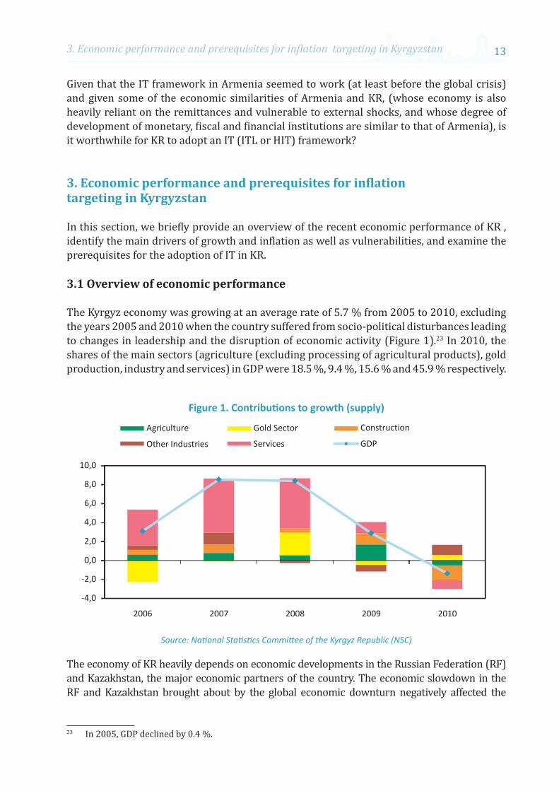
The Kyrgyz economy was growing at an average rate of 5.7 % from 2005 to 2010, excluding the years 2005 and 2010 when the country suffered from socio-political disturbances leading to changes in leadership and the disruption of economic activity (Figure 1).23 In 2010, the shares of the main sectors (agriculture (excluding processing of agricultural products), gold production, industry and services) in GDP were 18.5 %, 9.4 %, 15.6 % and 45.9 % respectively.
Figure 1. Contributions to growth (supply)
Source: National Statistics Committee of the Kyrgyz Republic (NSC)
The economy of KR heavily depends on economic developments in the Russian Federation (RF) and Kazakhstan, the major economic partners of the country. The economic slowdown in the RF and Kazakhstan brought about by the global economic downturn negatively affected the
23 In 2005, GDP declined by 0.4 %.

On the Possibility of Inflation Targeting in Kyrgyzstan14
economic performance of KR in 2009. Remittances from these countries fell from about 23 % of GDP in 2008 to around 16 % in 2009 (Figure 2). The inflow of FDI and demand for Kyrgyz exports also contracted sharply. As a result, economic growth slowed to 2.9 % in 2009 (Table 1).
Figure 2. Remittances as a share of GDP
Source: National Bank of the Kyrgyz Republic (NBKR).Notes: Remittances of individuals made through electronic systems.
The country was on path to recovery from the global economic crisis with GDP growth recorded at 16.4 % in the first quarter of 2010. Growth was mainly driven by higher gold production. The closure of international borders following the events of April and Junedisrupted agricultural production, trade and other services.24 As a result, real GDP decreased by 1.4 % in 2010 (Table 1). The economic contraction would have been more severe without expanded gold production. Economic recovery in the RF and Kazakhstan and ensuing higher migrant remittances (increased by an estimated 25 % relative to 2009) from these countries to the KR also helped ease the downward pressure on aggregate demand. Continuing economic growth in these countries in 2011 led to an increase of about 50 % in remittances from these countries to KR (Figure 2).
Table 1. Growth rates of GDP and sectors (in % to the corresponding period of the previous year)
2008 2009 2010GDP 7.6 2.9 -1.4Non-gold GDP 5.4 3.4 -1.9Agriculture 0.7 6.7 -2.8Construction 10.8 22.1 -22.8Industry 10.7 -8.1 11.3Services 10.7 2.3 -1.8
Source: NSC
24 The socio-political disturbances in Bishkek in April 2010 and the outburst of violent conflict in southern KR in June 2010 led to many casualties, substantial damages to infrastructure and buildings, weakening private sector confidence, contraction of liquidity in the banking system and massive stress on public finance.

153. Economic performance and prerequisites for inflation targeting in Kyrgyzstan
The inflation measure used in KR is based on consumer price index (CPI). Key staple items make up the majority of the CPI food basket accounting for 57.1 %.25 Food accounts for a large share of CPI basket (Table 2). Many of these items are produced locally, but supplemented with imports. Table 2 shows a high degree of food import dependence and high correlations between global food prices and domestic inflation, underscoring the channels for external shocks. Domestic prices broadly mirror global trends, but exhibit downward stickiness, a result of local market inefficiencies, domestic monopolies and limited global trade. As a result, high global food prices quickly pass-through to headline inflation and also affect core inflation.26
Table 2. CPI composition and correlation between global food prices and inflation (2010)
Kyrgyz RepublicFood share in CPI 57.1
of which Bread Products 19.5Energy share in CPI (fuel only) 6.9Correlation between Global Food Prices and
Headline Inflation 0.8Food Inflation 0.87
Food Share in imports (as of end 2009) 13.9Net food importer Yes
Source: Al-Eyd et al, 2012
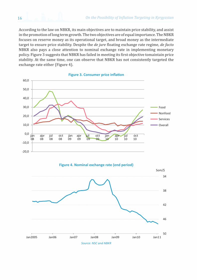
Inflation in KR has exhibited considerable volatility, especially food and services inflation (Figure 3). The surge in international food and fuel prices and political instability in 2010 explain the bulk of the recent hike in inflation.27 To sum up, inflation performance in recent years has been far from satisfactory.
During the same period, the country faced exchange rate policy challenges, which are illustrated in Figure 4. KR experienced periods of substantial nominal depreciation and appreciation. Despite the officially announced floating exchange rate regime, the National Bank of the Kyrgyz Republic (NBKR) de facto follows managed exchange rate policy by resisting those exchange rate movements that it considers undesirable. Given the relatively high exchange rate pass-through to domestic prices, and taking into account the fact that KR is a net importer of food and fuel, the depreciation of the local currency (starting in the second half of 2008) added significantly to headline inflation.
25 Major food staples in the CPI basket include bread, carrots, flour, onion, potatoes, rice, meat (sheep, beef and poultry), milk, eggs, vegetable oil and sugar. Ali Al-Eyd, David Amaglobeli, Bahrom Shukurov, and Mariusz. Sumlinski, “Global Food Price Inflation and Policy Responses in Central Asia,” International Monetary Fund (IMF) Working Paper No. 86, (Washington DC: IMF, March 2012).
26 Ibid.27 In January 2009, the Government doubled tariffs for electricity, heating and hot water, which were returned
to their 2008 levels in April 2010. This explains, to a large extent, the variability of services inflation from 2008 to 2010.
On the Possibility of Inflation Targeting in Kyrgyzstan16
According to the law on NBKR, its main objectives are to maintain price stability, and assist in the promotion of long term growth. The two objectives are of equal importance. The NBKR focuses on reserve money as its operational target, and broad money as the intermediate target to ensure price stability. Despite the de jure floating exchange rate regime, de facto NBKR also pays a close attention to nominal exchange rate in implementing monetary policy. Figure 3 suggests that NBKR has failed in meeting its first objective tomaintain price stability. At the same time, one can observe that NBKR has not consistently targeted the exchange rate either (Figure 4).
Figure 3. Consumer price inflation
jan apr jul oct jan apr jul oct jan apr jul oct
Figure 4. Nominal exchange rate (end period)
Source: NSC and NBKR

173. Economic performance and prerequisites for inflation targeting in Kyrgyzstan
Despite a variety of available monetary instruments, the NBKR mostly uses NBKR notes to withdraw liquidity and makes interventions in the foreign exchange market on both sides of the market to smooth out exchange rate developments. Other instruments are rarely used.28
Recent research by NBKR found little correlation between inflation and policy related variables such as monetary aggregates, foreign exchange rates and interest rates.29 The weakness in the interest rate transmission mechanism is mainly due to the relatively excessive liquidity of the banking sector. The NBKR also partially attributes this weakness to the low level of competition. As such, there is no clear relationship between NBKR’s policy rate and the bank’s lending rate. Another factor affecting the efficiency of monetary policy conduct is the high degree of dollarization. Since 2000, both foreign currency deposits and loans have fluctuated above 50 % of total deposits and loans respectively (Figure 5).
Figure 5. Foreign currency denominated deposits and loans, % of total deposits and loans
Source: NBKR
As for fiscal performance, during the period 2009 to 2011, the government opted for expansionary fiscal policy to mitigate the negative consequences of the global economic crisis and devastating effects of the internal crisis of 2010. As a result, the budget deficit widened from almost 0 % of GDP in 2008 to over 7 % of GDP in 2011 (Figure 6). The major bulk of fiscal imbalances were covered from external sources, concessional loans and grants extended by the donor community. For instance, in 2011, over 70 % of the fiscal gap was financed from external sources. Both global and internal crises also led to the increase in
28 The instruments include: NBKR notes offered weekly via a volume-based auction, with no cut off rate; NBKR repos/reverse repo auctions offered weekly, with government treasury bills as collateral; NBKR announces a cut of rate in addition to the volume; Direct purchases and sales of government treasury bills in the secondary market; Discount rate, which is considered the key policy rate and is set at the average of the last four rates determined in the weekly 28-day NBKR note auctions; Mandatory reserve requirements; Deposit facility; Overnight credits with the rate set at 1.2 times the rediscount rate; Lender of last resort (LOLR) facility; Intervention in the foreign exchange market and Swap operations in foreign exchange.
29 However, NBKR was not willing to disseminate the study.

On the Possibility of Inflation Targeting in Kyrgyzstan18
public external debt in recent years (Figure 7). The Government recently embarked on a medium-term fiscal consolidation programme that will help to reduce the size of the budget deficit, reliance on external finance and direct external funds to financing infrastructural projects. While there is no clear indication of fiscal dominance in KR, from 2010 to 2012, the monetary authorities had to tighten their monetary stance in view of higher government spending and increasing in-flow of remittances.
Figure 6. Fiscal indicators, % of GDP
Figure 7. Public external debt, % of GDP
Source: IMF and NBKR

193. Economic performance and prerequisites for inflation targeting in Kyrgyzstan
3.2 Examination of IT prerequisites in Kyrgyzstan
In this section we examine whether or not the country currently meets the widely-accepted economic and institutional prerequisites for the successful adoption of the full-fledged IT (FFIT) framework.
3.2.1. Central Bank independence and accountability and coordination between monetary and fiscal policies
The NBKR board meets every quarter to set general guidelines. Summaries are communicated twice a year to the Parliament, for information only. The NBKR releases a statement at the beginning of the year, which includes a non-binding indicative inflation target. However, no formal mechanisms of penalties and legal consequences for non-compliance with targets exist, which does not enhance NBKR’s credibility.
The independence of the CB is perceived as a key condition of successful inflation control. In general, the legal independence of NBKR is well established. NBKR is an independent institution under Kyrgyz law. One study 30 found that NBKR scores 0.89 (with 0 being very poor and 1 being very strong), which is the highest among KR and its neighbours Kazakhstan, Tajikistan and Uzbekistan. With regard to transparency, however, NBKR performed poorly with the score of 0.4, ranked second after Kazakhstan. Though analytical and statistical information is published, the poor transparency performance of NBKR is due to the fact that very little is disclosed regarding its policy making processes. Coordination between monetary and fiscal policies improved in recent years. The recent International Monetary Fund (IMF) country report for the KR conducted in December 2011 concludes that the Ministry of Finance and NBKR have been closely coordinating their policies. However, liquidity forecasting is still complicated due to the poor quality of inputs from the Ministry of Finance. There are no clear symptoms of “fiscal dominance.” However, there are some instances of interference from the executive and legislative branches of the government, and there are no legal limits imposed on lending to the government.
3.2.2. Vulnerability to external shocks and exchange rate pass-through
Kyrgyzstan is highly vulnerable to external shocks. Global food and energy price shocks are quickly transmitted to domestic prices (see Table 2). Relatively quick transmission of external (supply) shocks is also due to a (relatively) high exchange rate pass-through to domestic prices. The IMF estimates a reduced vector autoregression model (VAR) model for the determinants of inflation in the KR.31 The results suggest that a shock to broad money,
30 Ali Al-Eyd et al, (2012), using measures developed in Alex Cukierman, Central Bank Strategy, Credibility, and Independence: Theory and Evidence, (Cambridge, MA: MIT Press, 1992) and Christopher W. Crowe and Ellen E Meade, “Central Bank Independence and Transparency: Evolution and Effectiveness,” International Monetary Fund (IMF) Working Paper No. 08/119, (Washington DC: IMF, 2008.)
31 International Monetary Fund (IMF), IMF Country Report No. 09/209, (Washington DC: IMF, 2009). The variables of the VAR model include: international food price index, real GDP, price for services (as a proxy for administered prices), headline CPI, M2, and the som/dollar exchange rate.

On the Possibility of Inflation Targeting in Kyrgyzstan20
international food prices, the som/dollar exchange rate and service prices are all significant. In particular, a 10 % depreciation of the som leads to an almost immediate 2.5 % increase in inflation. The effects of the shock are significant for a period of three months. A 10 % increase in international food prices also results in a 2.5 % increase in inflation, with a lag of about four months, and the impact of the shock lasting for about seven months.
The economy is also highly susceptible to economic developments in the RF and Kazakhstan. According to unofficial statistics, these countries host over 500,000 labour migrants from KR. Remittances from these countries have fluctuated between 20 % and 30 % of GDP depending on economic conditions in these countries. Slow economic activity in these countries has a direct bearing on the Kyrgyz economy.
3.3.3. Financial sector development and stability
The financial system in the KR is underdeveloped and is dominated by banks. The Kyrgyz banking system comprises 22 commercial banks, out of which one is state-owned. At the end of -2010, private banks made up about 92 % of total assets in the banking sector. The stock market is at its rudimentary stage of development, with stock market capitalization of 1.7 % of GDP in the end of 2010 (Table 3).
Table 3. Financial system health, as of end 2010
Bank regulatory capital to risk weighted assets (in percent) 30.4Stock market capitalization to GDP (in percent) 1.7Bank assets to GDP (in percent) 27.6Domestic currency lending-deposit spread (percentage points) 18.3NPLs(Gross) to total loans 15.8
Source: NBKR
The latest World Bank(WB) and IMF 2007 Financial Sector Assessment Programme report found that Kyrgyzstan had a sound base of prudential requirements for banks, supervision and accounting standards, and that good progress had been achieved in the supervision of the banking system. The report’s reassessment of Basel Core Principles for Effective Banking Supervision concluded that NBKR observed good practices. More specifically, it found major improvements in the legislative framework and in supervisory practices. However, recent experience in the banking sector, following the events of 2010, revealed weaknesses in the legal framework for early intervention and the resolution of problems in the sector. Comprehensive reform of the legal framework governing the financial sector will be important to remedy these shortcomings and ensure that the supervisory authority is better placed to take resolute action in the future. The IMF recently concluded that despite recent difficulties financial sector stability has been maintained.32 Overall, the banking system remains adequately liquid and capitalized.
32 International Monetary Fund (IMF), IMF Country Report No. 11/354, (Washington DC: IMF, 2011).

214. Small Open Economy Model
To summarize, KR has not met most of the commonly-accepted preconditions for the successful adoption of the FFIT, due to de facto lack of CB independence and credibility and the absence of accountability; weak monetary transmission mechanisms; high degree of dollarization; a large informal sector; an underdeveloped financial market; high vulnerability to external shocks; and limited technical capacity of the NBKR.33 It would therefore be premature for the country to adopt a FFIT framework.
However, many of successful IT implementing countries have not had all the preconditions in place prior to adopting an IT regime. Moreover, the results of the modeling exercise in the next section clearly suggest that the economy of KR could benefit if the NBKR responds aggressively to inflation fluctuations, as well as to nominal exchange rate fluctuations , and adopts a hybrid IT framework.
4. Small Open Economy Model
In the previous section we established that the NBKR has neither consistently targeted inflation or exchange rate fluctuations. Is such a policy optimal and what would the appropriate monetary arrangement be for an emerging economy like KR? To address this question, we built a small open economy dynamic stochastic general equilibrium (DSGE) model that is calibrated to KR and incorporates important economic features of the economy, such as reliance on migrant remittances and high exposure to external shocks. The model allows for the conduct of welfare analysis and for the comparisons across alternative monetary and fiscal policy combinations. There are a number of features that distinguish our model from others’.34 First, the fiscal side of the economy is modeled explicitly.35 This allows for interaction between alternative monetary and fiscal policy rules. More specifically, we consider fiscal regime based on the deficit rule that is implicitly targeted by the Kyrgyz fiscal authority.36 Second, we depart from the widespread practice in the field that assumes undistorted steady states and perfect
33 According to some estimates the size of the informal economy constitutes about 50 % of GDP.34 Recently, there have been many SOE models built for the analysis of alternative monetary and exchange
rate regimes. For example, see Jordi Gali and Tomasso Monacelli, “Monetary Policy and Exchange Rate Volatility in a Small Open Economy,” Review of Economic Studies no. 72, (2005): 707-734; and Tomasso Monacelli."Monetary Policy in a Low Pass-Through Environment," Journal of Money Credit and Banking, vol. 37 no. 6, (2005): 1047-1066.
35 Fiscal policy is thought to be of little consequence as far as inflation is concerned. This is based on the beliefby some that inflation is a purely monetary phenomenon. However, recent findings suggest that fiscal policy has an impact on the price level. For example, see Michael Woodford. “Monetary Policy and Price-Level Determinacy in a Cash-in-Advance Economy," Economic Theory no. 4, (1994): 345-380; Michael Woodford, “Price-level Determinacy without Control of a Monetary Aggregate," Carnegie-Rochester Conference Series on Public Policy no. 43, (1995): 1-46; Michael Woodford, “Control of the Public Debt: A Requirement for Price Stability?" National Bureau of Economic Research (NBER) Working Paper 5684. (Cambridge: NBER, 1996); Michael Woodfored, “Public Debt and the Price Level," Working Paper, (Princeton: Princeton University, 1998); and Michael Woodford, “Fiscal Requirements for Price Stability," Journal of Money Credit and Banking no. 33, (2001): 669-728.
36 The Extended Credit Facility Programme of the IMF requires the Kyrgyz Republic to follow prudent fiscal policy and avoid excessive budget deficits.

On the Possibility of Inflation Targeting in Kyrgyzstan22
risk sharing. Instead, we work with distorted steady states and incomplete assets markets. We use the algorithm developed by Schmitt-Grohe and Uribe37 to compute second order approximations to policy functions and to calculate conditional welfare outcomes across alternative combinations of monetary and fiscal policies. Below, we provide the main building blocks of the model which build upon earlier work.38
The model features two countries, home and foreign. The latter is also referred to as “the rest of the world.” The foreign country is not modeled explicitly; equations describing the foreign economy mainly enter the model in terms of the exogenously given stationary autoregressive of order one (AR (1)) processes. In the home country, households maximize expected lifetime utility, taking prices and wages as given. The production process in the home country consists of two stages. In the first stage, home firms produce intermediate tradable and non-tradable goods in a monopolistically competitive environment. The prices in both tradable and non-tradable intermediate goods sectors are sticky. The capital in both sectors is assumed to be fixed and there is no investment. Therefore, the production technology in these sectors is assumed to feature decreasing returns to scale in labour. In the second stage, the economy produces a final good from domestic non-tradable, domestic tradable and foreign intermediate goods composites. The final good is produced in a perfectly competitive environment, and is then used for private and government consumption.
Households
In the home country, there is an infinitely-lived representative consumer, who maximizes his/her expected lifetime utility
1 1
00
( )max E1 1
t t t
t
C Hρ ψ
βρ ψ
− +∞
=
− − +
∑ ,
subject to a flow budget constraint:
PtCt(1+τct)+etBF,t+BH,t = et(1+iF,t–1)BF,t–1+(1+it–1)BH,t–1+(1–τl
t)(WH,tHH,t +WN,tHN,t)+Пt+etTRt (1)
Households receive labour income subject to the average tax rate, τl, from supplying labour to tradable and non-tradable sectors in line with
Ht = HH,t + HN,t (2)
There is also a tax on consumption, τc. Households receive profits, П, from firms that produce intermediate goods. It is assumed that these firms are owned by consumers. Corporate
37 Stephanie Schmitt-Grohé and Martín Uribe, “Solving Dynamic General Equilibrium Models Using Second Order Approximation to the Policy Function,” Journal of Economic Dynamics and Control no. 28, (2004): 755-775.
38 Nurbek Jenish, "Choice of Exchange Rate Regime for Partially Dollarized Developing Economies," Central European University Working Paper (2008a.); and Nurbek Jenish, "Optimal Monetary and Fiscal Policy Rules for New European Union (EU) Countries on Their Road to Euro," Central European University Working Paper (2008b).

234. Small Open Economy Model
taxation is not considered in this model since it is most relevant for the evolution of investment, which is absent in the model. BH are domestic currency denominated government bonds held by consumers. Households also have an access to foreign currency denominated bonds, BF. e is a nominal exchange rate expressed as the number of units of local currency required to purchase one unit of foreign currency. TRt are net foreign transfers (migrant remittances) which are subject to shock.
Let us introduce a new notation: CPI inflation, πt+1 = Pt+1 / Pt; tradable and non-tradable goods sectors’ inflation, πi,t+1 = Pi,t+1 / Pi,t for i = N,H; real wage, wt = Wt / Pt, where Wt = WH,t = WN,t. The last equality comes from the household’s optimisation problem, since the labour is mobile across sectors.
Then, the household’s optimisation gives the following first order conditions (FOCs) written in real terms.
Euler equation:
1
1 1
1 1 (1 ) 1 1
ct t
t tct t t
CE iC
ρτβτ π
−
+
+ +
+ + = +
(3)
Uncovered interest parity (UIP) equation under consumption capital asset pricing model (C-CAPM):
1 1,
1 1
1 1 (1 ) 1 1
ct t t
t F tct t t t
C eE iC e
ρτβτ π
−
+ +
+ +
+ + = +
(4)
Labor supply equation:
1 01
lt
t t tct
C Hρ ψτωτ
− −− =
+, i = N,H
(5)
Final good market
The domestic economy produces one final good, Y, which is manufactured from a non-tradable intermediate goods composite and intermediate tradable goods composite. The final good is then split between private and government consumption. The labour market is assumed to be perfectly competitive. We also assume there are no barriers for trade and no transportation costs.
The final good is manufactured according to the following Cobb-Douglas production technology:
1
1 (1 )
N TY YYγ γ
γ γγ γ
−
−=−
,

On the Possibility of Inflation Targeting in Kyrgyzstan24
where YN is an aggregate of domestically produced intermediate goods, which is given by:
1 11
0
( ) N NY y i diω ωω ω−
−
= ∫ .
yN is an output of an individual firm producing intermediate non-tradable goods. YT is a composite index consisting of both domestic and foreign intermediate tradable goods aggregates and is given by:
1
1 (1 )
H FT
Y YYε ε
ε εε ε
−
−=−
.
Domestic and foreign intermediate tradable aggregates, in turn, are:
111
0
( ) H HY y i diη ηη η−
−
= ∫ , and
121
1
( ) F FY y i diµ µµ µ−
−
= ∫ , respectively.
One can use the above definitions of final good, non-tradable and tradable intermediate goods aggregates to define their respective price indexes.
The aggregate price index (CPI):
P = P γN PT
1–γ
Tradable price index:
PT = P εH PF
1–ε
where
11 1
1
0
( )H HP p i diη
η−
− = ∫ and
12 1
1
1
( )F FP p i diµ
µ−
− = ∫ .
Non-tradable price index:
11 1
1
0
( )N NP p i diω
ω−
− = ∫ .
Under the assumption of perfect competition in the final good market, one can easily derive the following demand functions. Demand for individual tradable and non-tradable intermediate goods are:
( )( ) HH H
H
P iy i YP
η−
=
,

254. Small Open Economy Model
( )( ) FF F
F
P iy i YP
µ−
=
,
( )( ) NN N
N
P iy i YP
ω−
=
.
Demand for tradable and non-tradable composites are given as:
1
HH T
T
PY YP
ε−
=
,
1
(1 ) FF T
T
PY YP
ε−
= −
,
1
(1 ) TT
PY YP
γ−
= − ,
1N
NPY YP
γ−
= .
Intermediate goods producers
Every variety of tradable and non-tradable goods is produced by a single firm in a monopolistically competitive environment. Firm i ! [0,1] produces good yt(i) using labor, Ht(i). Each variety is then used in the production of the final good. The production function of a representative firm in both tradable and non-tradable sectors exhibits decreasing returns to scale (DRS) in labour and is subject to temporary productivity shocks:
Yj,t(i) = Aj,tHj,t(i)αj , 0 < αj < 1 and j=H, N.
Aj,t is an exogenous productivity parameter subject to shocks and is common for all producers in sector j. The log of the technology parameter follows an AR(1) process:
ln(Aj,t / Aj) = φln(Aj,t–1 / Aj) + ςj,t, (6)
where Aj is steady state value of productivity for j=H, N, ς is a zero mean independently identically distributed (i.i.d.) productivity shock and 0 ≤ φ < 1.
We follow Schmitt-Grohe and Uribe39 and introduce money into the model by assuming that firms’ wage payments are subject to a cash-in-advance (CIA) constraint that requires that a certain fraction of the wage bill should be backed with monetary assets.40 This is necessary to
39 Stephanie Schmitt-Grohé and Martín Uribe, “Optimal Simple and Implementable Monetary and Fiscal Rules,” Journal of Monetary Economics no, 54, (2007).
40 As an alternative, one can (i) make real monetary balances enter the utility function of households; (ii) impose a CIA constraint on the households’ consumption, and (iii) impose CIA constraints both on the wage bill and private consumption.

On the Possibility of Inflation Targeting in Kyrgyzstan26
allow the government to extract seignorage revenues. Though seignorage revenues constitute a small fraction of total government revenues in industrialized countries, one should not neglect them, especially, if one studies interactions between monetary and fiscal policies. Monetary policy impacts the real value of outstanding government debt (provided that much of public debt is nominal), through its effects on the price level and real debt service.41
For simplicity, let us omit sector and firm subscripts. Then the CIA constraint can be written as:
Mt ≥ vWtHt. (6)
Price Setting in the non-tradable sector
Prices are assumed to be sticky as per Calvo and Yun42 in both tradable and non-tradable sectors. Each period, a fraction θ ! [0,1) of randomly chosen firms is not allowed to change the nominal price of the good that it manufactures. The remaining (1 – θ) firms set prices optimally. In the calibration procedure θ is assumed to be the same for both sectors. However, it can easily be made different across sectors and will not affect the qualitative nature of results.43 Let us suppose that firm i gets to choose price P~N,t. Let us also drop, for simplicity, index i. Then, the firm’s profit maximization problem can be written:
,, ,
s=tmax
N t
s tt s N sP
θ σ∞
− Π∑
where σt,s is a pricing kernel, which is assumed to be equal to the household’s intertemporal marginal rate of substitution in consumption. The firm’s profits are given as:
ПN,s = P~N,s aN,s – WtHN,t – (1 – (1 + it)–1)MN,t
where aN,s is a domestic absorption of domestically produced non-tradable goods, which is defined below. In the derivation of the last expression, we use the following assumptions. Let us assume that firms in both sectors also have a choice of holding bonds denoted Bfirm,t (again, we drop firm and sector subscripts). Then, a period-by-period budget constraint of a firm can be written as:
Mt + Bfirm,t = Ptat – WtHt + Mt–1 + (1 + it–1)Bfirm,t–1.
41 Michael Woodford, “Fiscal Requirements for Price Stability," Journal of Money Credit and Banking no. 33, (2001): 669-728.
42 Guillermo Calvo,”Staggered Prices in a Utility-Maximizing Framework," Journal of Monetary Economics no. 12, (1983): 383-398; and Tak Yun, “Nominal Price Rigidity, Money Supply Endogeneity, and Business Cycles," Journal of Monetary Economics no. 37, (1996): 345-370.
43 The next section, describes our experiment in which we decreased the degree of price stickiness in the tradable sector. The results clearly show that this does not affect the qualitative nature of the findings.

274. Small Open Economy Model
Following Schmitt-Grohe and Uribe,44 we assume that the firm’s initial wealth is nil. That is, M–1 + (1 + i–1)Bfirm,–1 = 0. Moreover, we assume that firms hold no financial wealth at the beginning of any period, or Mt + (1 + it)Bfirm,t = 0 for all t. These assumptions, along with the firm’s budget constraint, imply the firm’s profit function given above.
From the cost minimisation problem of the firm, one can get an expression for marginal cost in the non-tradable sector, which is identical across the firms in the non-tradable sector since they face the same factor price, have access to the same production technology, and do not face idiosyncratic productivity shocks:
1
(1 )1
NN N
iWiMC
A H α
ν
α −
++= . (8)
Then, the firm’s optimization with respect to P~N,t gives the following FOC:
1
, , ,t , ,
s=t , , ,
1E 0N t N t N ss tt s N s
N s N s N s
P P MCa
P P P
ωωθ σ
ω
− −∞
− − + = ∑
. (9)
We limit our attention to a symmetric equilibrium at which all firms that happen to change their price in each period choose the same price. Therefore, one can use the definition of the non-tradable price index to obtain:
θπ ω N –,
1t + (1 – θ) P
∼∧ 1 N
–,
ωt = 1, (10)
where P∼∧
N = P~
N / PN is the relative price of any non-tradable good whose price was changed in period t relative to the composite non-tradable good. The standard practice in the neo-Keynesian literature is then to log-linearize equations (9) and (10) to derive the standard (linear) New Keynesian Phillips curve that involves inflation and marginal costs. However, since the long run inflation is not zero we follow a different approach proposed by Schmitt-Grohe and Uribe.45
We can define two new auxiliary variables x1
t and x2t to get rid of the infinite sum in (9) and
keep the nonlinear structure. Further, the problem can be cast in a recursive way.
Let
44 Stephanie Schmitt-Grohé and Martín Uribe, (2007).45 Ibid
Another shortcoming of the approach that involves log-linearization is the necessity to make additional assumptions if one is to accurately calculate welfare from first order approximation to the equilibrium conditions. The steady state in this model is distorted with the distortions coming from monopolistic competition. Therefore, in order to undo the distortions, one has assume the existence of factor-input subsidies financed by lump sum taxes that would ensure the competitive long-run employment level.

On the Possibility of Inflation Targeting in Kyrgyzstan28
1 1 1
, , , , , ,1, , , , ,
s=t s=t+1, , , , , ,
N t N s N t N t N t N ss t s tt t t s N s N t t t s N s
N s N s N t N t N s N s
P MC P MC P MCx E a a E a
P P P P P P
ω ω ω
θ σ θ σ− − − − − −
∞ ∞− −
= = +
∑ ∑
1 1 1
, , , , 1 ,1, , 1 1 1, ,
s=t+1, , , 1 , ,
N t N t N t N t N ts tN t t t t t t s N s
N s N t N t N s N t
P MC P P MCa E E a
P P P P P
ω ω ω
θ σ θ σ− − − − − −
∞+− −
+ + ++
= +
∑
1
, ,1 1, , , 1 1
, , 1, 1
ˆ 1ˆ ˆN t N t
N t N t t t t tN t N tN t
MC PP a E x
P P
ω
ω θ σπ
− −
− −+ +
++
= +
. (11)
Similarly, let
,2 2, , , , , , 1 1
s=t , 1, 1
ˆ 1ˆ ˆˆ
N ts tt t t s N t N s N t N t t t t t
N tN t
Px E P a P a E x
P
ω
ω ωθ σ θ σπ
−∞
− − −+ +
++
= = +
∑
. (12)
Using these two auxiliary variables, we can rewrite (9) as:
1 2
1t tx xωω
=−
. (13)
At equilibrium, domestic absorption is given by aN = YN .
Integrating over all firms, one can obtain:
1,
, ,,0
( ) N N t
N t N t NN t
P iA H Y di
P
ω
α
−
= ∫
Following Schmitt-Grohe and Uribe (2007), let us introduce new variable 1
,,
,0
( )N tN t
N t
P is di
P
ω−
= ∫ . Then one can derive the law of motion for sN,t:
1, , , 1 , 22
,, , , ,0
( ) (1 ) (1 ) (1 ) ...N t N t N t N t
N tN t N t N t N t
P i P P Ps di
P P P P
ω
θ θ θ θ θ−
− − = = − + − + − +
∫
,
,, 1
0 ,
ˆ (1 ) (1 )N t
N t jjN t
j N t
PP s
P
ω
ω ωθ θ θ θπ−
∞− −
−=
= − = − +
∑
. (14)
The state variable sN,t represents the resource costs induced by the presence of price dispersion.46 Therefore, the resource constraint in the nontradable sector is given by:
YN,t = AN,t H αN,t / sN,t. (15)
46 Ibid for a more detailed discussion of ,N ts .

294. Small Open Economy Model
Price setting in the tradable sector
Analogously, the firm’s minimization problem gives a similar expression for the marginal cost in the tradable sector:
1
(1 )1
HH H
iWiMC
A Hα
ν
α −
++= . (16)
Using the definition of the intermediate tradable domestic goods index one obtains:
θπ η H
–,
1t + (1 – θ) P
∼∧ 1 H
–,
ηt = 1. (17)
where P∼∧ H = P
~H / PH is the relative price of any domestically produced tradable good whose
price was changed in period t relative to the aggregate tradable index.
We can follow the same steps that were used for the non-tradable sector to obtain the following equations that characterize price setting in the tradable sector.
11
, , , ,3 1 3, , , , , 1 1
s=t , , , , 1, 1
ˆ 1ˆ ˆH t H t H t H ts t
t t t s H s H t H t t t t tH t H t H t H tH t
P MC MC Px E a P a E x
P P P P
ηη
ηθ σ θ σπ
− −− −∞
− − −+ +
++
= = +
∑
. (18)
As before:
,4 4, , , , , , 1 1
s=t , 1, 1
ˆ 1ˆ ˆˆ
H ts tt t t s H t H s H t H t t t t t
H tH t
Px E P a P a E x
P
η
η ηθ σ θ σπ
−∞
− − −+ +
++
= = +
∑
. (19)
3 4
1t tx xηη
=−
. (20)
Absorption of tradable goods is given by aH = YH + C *H. Where the last term, C *H , represents consumption of domestically produced tradable home goods by the foreign country. In what follows, the starred variables correspond to the foreign country.
Foreign demand
Let us make some assumptions about the foreign country. Foreign demand for traded home
variety i is given by
* 1* * *
*
( )( ) H HH
H t t
P i PC i CP e P
η
ε−−
=
. Where ε* is a share of home goods in
foreign consumption. We assume producer currency pricing, that is, producers cannot price

On the Possibility of Inflation Targeting in Kyrgyzstan30
discriminately between markets. Since home is a small open economy, we can do the following
simplifications: C *t = Y *t , P*F,t = P*
t . Then,
11, ,* * * * *
, * *,
H t H tH t t t
t t t F t
P PC C Y
e P e Pε ε
−− = =
.
Similar to the non-tradable sector equilibrium, equations describing equilibrium in the home tradable sector are:
YH,t + C *H,t = AH,t H αH,t / sH,t . (21)
sH,t = (1 – θ) P∼∧ – η + θπ ηH,t sH,t–1 . (22)
where 1
,,
,0
( )H tH t
H t
P is
P
η−
= ∫ . The state variable iF,t represents the resource costs in the tradable
sector arising from the presence of price dispersion.
Closing the model and equilibrium conditions
We assume that the interest rate at which a home country household can borrow (lend) in foreign currency, iF,t , is set equal to the foreign interest rate plus a premium, which is an increasing function of the country’s real foreign debt:47 iF,t = i *t + Y[exp(dt – d) –1], where Y > 0 and dt is holdings of real foreign currency denominated bonds at time t, and d is a steady state level of debt.
The aggregate resource constraint is:
Yt = Ct + Gt . (23)
The balance of payments equation can be written as:
et BF,t = (1 + iF,t–1)et BF,t–1 – C *H,t PH,t – etTRt + PtYt . (24)
Rest of the world
In the foreign block, it is assumed that output, inflation and interest rate follow exogenous AR(1) processes:
ln(π*t / π
–*) = ρπ ln(π*t–1 / π
–*) + επ , (25)
ln(Y *t / Y*) = ρY ln(Y *t–1 / Y
*) + εY , (26)
ln((l + i*t ) / (l + i–*)) = ρI ln((l + i*
t–1 ) / (l + i–*)) + εi , (27)
where εi , εi and εY are i.i.d. processes and are neither correlated with each other nor with any other shocks in the model. The bar over a variable denotes its steady state value.
47 Stephanie Schmitt-Grohé and Martín Uribe. "Closing Small Open Economy Models," Journal of International Economics, Elsevier, vol. 61(1), (2003).

314. Small Open Economy Model
Government
The consolidated government prints money, issues one-period nominally risk-free bonds, collects taxes, and faces an exogenous government expenditure stream.
Mt + BH,t + Tt = (1 + it )BH,t–1 + Mt–1 + PtGt , (28)
where Tt are total tax revenues and are given as: Tt = τ ct CtPt + τ l
t Wt(HH,t + HN,t ). Real tax collections can be written as: τt = τ c
t Ct + τ lt (HH,t + HN,t )Wt / Pt.
It is also assumed that public consumption Gt follows the following AR(1) process:
ln(Gt / G–) = ρg ln(Gt–1 / G
–) + εg,t , (29)
where G– is a steady state level of government consumption, and 0 ≤ ρg < 1.
Real GDP is given by:
,,
F tt t F t
t
Pgdp Y Y
P= − . (30)
We also assume remittances to follow AR(1) process:
ln(TRt / TR) = ρtr ln(TRt–1 / TR) + εtr,t , (31)
where TR is a steady state level of remittances.
The fiscal authority follows a rule based on the deficit requirement:
τ jt = τ j + Ωl (Gt – τt + it–1 BH,t–1 / Pt – κl gdpt ) / gdpt , (32)
where j=C,H. The government increases consumption or labour income tax rate if the deficit-to-GDP ratio goes above the target level κl.
The monetary authority can employ one of the three rules that are based on the interest rate: IT, IT with managed float (or HIT regime), and fixed exchange rate regime. Under all three rules, the CB uses interest rate as its main policy instrument. All three monetary regimes can be described by an open-economy version of the Taylor rule:48
ln((l+it ) / (1 + i–)) = ω– ln((l+it–1 ) / (l+i–)) + (l – ω–) [Ωπ ln(πt / π–) + Ωe ln(et / e
–)]
where bars over variables denote their steady state values. Ωe = 10–3 and Ωπ ≥ 0 represents the
IT regime. Ωe > 0 and Ωe = 103 corresponds to IT with managed float case. Ωe = 103 and Ωπ = 0
describes the fixed exchange rate regime. ω– is the extent of interest rate inertia.
48 In specifying the interest rate rule, we do not make interest rate responsive to the deviation of the output from its potential level in view of negligible welfare improvements when interest rate is responsive to output gap. See Stephanie Schmitt-Grohé and Martín Uribe, (2007).

On the Possibility of Inflation Targeting in Kyrgyzstan32
Equilibrium
Formally, equilibrium can be defined as a set of stationary processes Ct , Ht , mt , wt ,mcH,t , Yt , mcN,t , x 1t , x 2t , x 3t , x 4t , bH,t , dt , πt , πH,t , πN,t , P
∼∧
H,t , P∼∧
N,t , sH,t , sN,t , St , Qt , et , it and τ jt for t ≥ 0 that maximize (for the definitions of transformed variables see Annex A):
1 1
00
( )E1 1
t t t
t
C Hρ ψ
βρ ψ
− +∞
=
− − +
∑ ,
subject to the competitive equilibrium conditions: (1), (3)-(5), (7), (8), (11) - (13), (15), (16), (18) - (21), (23), (24), (28), (30), (A.22) – (A.24) provided in the Annex, which are all written in real terms; (2), (10), (14), (17), (22); fiscal rule (32); and exogenously given stochastic processes (6), (25)-(27), (29) and (31).
Solution algorithm and welfare measure
Most research dealing with the evaluation of alternative monetary and fiscal policies rests on the log-linear approximation of the equilibrium conditions – the policy functions - and consequent second order approximation of the welfare function. The choice of unconditional expectation is mostly due to its advantages of computational simplicity. This approach may yield accurate results under certain simplifying assumptions, such as restrictive preferences specifications and access to government subsidies. In general, for such an approach to give correct results up to the second order, it requires the solution to the equilibrium conditions also be accurate up to the second order. In this paper, we compute second order approximations to the policy functions and the welfare based on the system of first order and equilibrium conditions. We use the algorithm developed by Schmitt-Grohé and Uribe.49 We follow them and assume that in initial state all state variables are at their deterministic steady states. Alternative policy regimes are evaluated by the conditional expectation of the discounted lifetime utility.
In choosing the optimal policy regime, denoted by r, the benevolent government chooses a policy regime that maximizes the expected lifetime utility of a representative household:
1 1
00
( )E1 1
t t t
t
C Hρ ψ
βρ ψ
− +∞
=
− − +
∑ .
We can define the welfare associated under the optimal policy regime conditional on a particular state of the economy in period 0 as:
0 00
( , )r t r rt t
tV E u C Hβ
∞
=
= ∑ .
49 Stephanie Schmitt-Grohé and Martín Uribe, (2004).
334. Small Open Economy Model
Let us denote an alternative policy regime by a. Similarly, the conditional welfare associated with policy regime a can be defined as:
0 00
( , )a t a at t
tV E u C Hβ
∞
=
= ∑ .
It is assumed that economy begins at time zero, at which all variables of the system are equal to their respective initial values. We further assume that the economy begins from the same state and grows at the same rate under the two alternative policy regimes. This delivers a constrained optimal policy regime associated with a particular initial state of the economy.50
Let λc denote the welfare cost of adopting policy regime a instead of the optimal policy regime r conditional on a particular state of the economy in period zero. λc is defined as the fraction of regime r’s consumption process that a representative household is willing to give up to be as well off under the regime a as under regime r. Then, λc can be implicitly defined by:
0 00
((1 ) , )a t c r rt t
tV E u C Hβ λ
∞
=
= −∑ .
Using the definitions above and ρ = 1, one can further rewrite this expression as:
0 0ln(1 )
1
ca rV V λ
β−
= +−
.
Now, we can derive a direct formula for calculating the welfare cost measure of adopting regime a instead of regime r :
λc = (1 – exp((V a0 – V r0 )(1– β)))x100%.
Parameterization
The calibrated parameters used in the paper are presented in Table 4. The time period in the model is one quarter. Therefore, we set β = 0.99. The risk aversion parameter, Y, is set equal to 1.51 We follow Christiano and others and set ψ = 1.52 The share of intermediate non-tradable and tradable goods index in the production of the final good is set to be equal 0.5, which is approximately true for KR. The share domestic tradable intermediate goods composite in the production of the tradable index is also set equal 0.5. Following Schmitt-Grohe and Uribe,53 the fraction of firms that cannot change their price in any given quarter is set at 2/3, meaning that on average, firms change their prices every three quarters. We also
50 In principle, the welfare ranking of alternative exchange rate arrangements might depend upon the initial value (distribution) of the state vector.
51 We tried higher values of risk aversion parameter, but it did not change the qualitative nature of results.52 Lawrence Christiano, Martin Eichenbaum and Charles Evans. "Sticky Price And Limited Participation
Models of Money: A Comparison," European Economic Review, Elsevier, vol. 41(6), (1997), 1201-1249.53 Stephanie Schmitt-Grohé and Martín Uribe, (2007).

On the Possibility of Inflation Targeting in Kyrgyzstan34
allow for lower price stickiness in the tradable sector, 1/3, and show that this does not affect the qualitative nature of the results. The degree of monopolistic competition in both tradable and non-tradable sectors is fixed at 5, which implies that the steady state markup of prices over marginal costs is 25 %.
The fraction of the wage bill that should be backed with monetary assets is given a value of 0.6, which is similar to Schmitt-Grohe and Uribe.54 The parameter determining the size of an interest rate premium on foreign borrowing, Y, is set at 0.0004, which is also needed to ensure stationarity in net foreign assets position. Decreasing returns to scale (DRS) parameter in both tradable and non-tradable sectors is given value of 0.8.55
Following Natalucci and Ravenna, AR(1) coefficients in the exogenous processes describing foreign interest rate are set at 0.9, respectively, and their corresponding standard deviations at 0.0025.56
For the variance and persistence of technology shocks, we use common values employed in the real business cycle literature. Variance is set 0.012, and persistence parameter is set equal 0.9.
The steady state ratio of remittances to GDP is set at 20 %, which is roughly the average of the last five years. For the remittances and government AR(1) processes, we estimated persistence coefficients and standard deviations using deseasonalised and Hodrick-Prescott (HP) detrended quarterly series for Kyrgyzstan. For the estimation of persistence and standard deviation of shocks for foreign output and foreign inflation AR(1) processes, we used Russian deseasonalized and HP detrended quarterly series, since the RF is the main economic partner of the country.
The desired deficit-to-GDP ratio is set at 3 %. This is an implicit target set by the Government of the KR. Steady state consumption and labour income taxes are set at 0.2 and 0.3, respectively, which are approximately the effective rates in the country. Interest rate inertia parameter is set at 0.8, which is a commonly used value in the literature.
Given the parameters above, the steady state share of imported intermediate goods constitute around 52 % of consumption. The steady state level of foreign debt was set at around 110 % of steady state GDP.57
54 Ibid.55 Lowering the value of this parameter did not change the qualitative nature of the results.56 Fabio Massimo Natalucci and Federico Ravenna. “Monetary Policy Choices in Emerging Market Economies:
the Case of High Productivity Growth,” Journal of Money, Credit and Banking, forthcoming.57 In this type of model, the steady state level of foreign debt is usually indeterminate. Therefore, it has to
be assigned the value exogenously. During the period 2000-2010 the average aggregate external debt in Kyrgyzstan constituted around 90 % of GDP. We expect that this ratio will increase in the coming years. The country plans to attract significant external resources for the construction of a number of hydropower stations and finance large-scale energy projects.

354. Small Open Economy Model
Table 4. Model parameterization
Para-meter Value Description
β 0.99 Quarterly subjective discount rate
ρ 1 Risk aversion parameter, C1–ρ / (1 – ρ) – H1+ψ / (1 + ψ)
1/ψ 1 Labor supply elasticity
γ 0.5 Share of tradable and nontradable intermediate goods indexes in the production of
final good, Y = Y γN Y T1–γ / (γγ (1 – γ)1–γ
ω 5 Degree of monopolistic competition in the nontradable intermediate domestic goods market
η 5 Degree of monopolistic competition in the domestic intermediate nontradable goods market
ε 0.5 Share of tradable intermediate domestic and foreign goods in the production of the
tradable index, YT = Y εH Y F1–ε / (ε ε (1 – ε)1–ε)
αH 0.8 DRS parameter, in the production function of domestic tradable intermediate goods, Y = AHαH
αN 0.8 DRS parameter, in the production function of domestic tradable intermediate goods, Y = AHαN
τ c 0.2 Steady state value of consumption tax
τ l 0.3 Steady state value of labor income tax
φ 0.9 Parameter in AR(1) productivity process ln(Aj,t ) = φ) ln(Aj,t–1 / A) + ςj,t , j=N, H
ν 0.6 Fraction of the wage bill that should be backed with monetary assets M ≥ vWH
θ 2/3 Parameter describing degree of price stickiness
ρπ 0.3 AR(1) coefficient in foreign inflation process, ln(π*t / π
–*) = ρπ ln(π*t –1 / π
–*) + επ
ρY 0.84 AR(1) coefficient in foreign output process, ln(Y *t / Y–*) = ρY ln(Y *t –1 / Y
–*) + εY
ρI 0.9 AR(1) coefficient in foreign interest rate process, ln((1 + i*
t ) / (1 + i–*)) = ρI ln((1 + i*t–1 ) / (1 + i–*)) + εi
ρg 0.24 AR(1) coefficient in government consumption process, ln(Gt / G–) = ρg ln(Gt–1 / G
–) + εg,t
ρtr 0.7 AR(1) coefficient in remittances process, ln(TRt / TR) = ρtr ln(TRt–1 /TR) + εtr,t
κ1 0.03 Target deficit-to-GDP ratio, τ jt = τ j + Ω1(Gt – τt + it–1 BH,t–1 / Pt – κ1gdpt ) / gdpt , j=C,L
ω– 0.8 Interest rate inertia parameter,ln((1 + it ) / (1 + i–)) = ω– ln((1+it–1 ) / (1 + i–)) + (1– ω–) [Ωπ ln(πt / π
–) + Ωe ln(et / e–)]
Y 0.0004 Foreign interest rate premium parameter, iF,t = i*t + Y [exp(dt – d) – 1]
σς j 0.01 Standard deviation of technology shock
σG 0.1 Standard deviation of government expenditure shock
σ*i0.0025 Standard deviation of foreign interest rate shock
σ*Y0.06 Standard deviation of foreign output shock
σ*π 0.12 Standard deviation of foreign inflation shock
σtr 0.11 Standard deviation of remittances shock

On the Possibility of Inflation Targeting in Kyrgyzstan36
5. Results
This section presents the results of conditional welfare estimations under alternative monetary arrangements. The alternative regimes are based on the augmented open economy version of Taylor rule:
ln((1 + it ) / (1 + i–)) = ω– ln((1+it–1 ) / (1 + i–)) + (1– ω–) [Ωπ ln(πt / π–) + Ωe ln(et / e
–)]
Depending on the values of reaction parameters Ωe and Ωπ, one can specify: (i) IT regime, with Ωe = 10–3 and Ωπ > 0 (here Ωe is assigned small positive value in order to ensure stationarity of nominal exchange rate, which will otherwise be indeterminate); (ii) Hybrid IT regime, with Ωe > 0 and Ωπ > 0. In this case, the CB reacts to the deviations of inflation and nominal exchange rate from their desired targets. We assigned a value of unity to Ωe when computing the welfare outcomes under this regime.58 (iii) Fixed exchange rate regime, Ωe = 103 and Ωπ = 0.
The fiscal authority follows a budget deficit rule, given by equation (32). In implementing the rule, the authority can use either consumption or labour income tax as an instrument. All together we compute conditional welfare for six alternative monetary and fiscal policy combinations.
We compute conditional welfare outcomes in the interval [0, 3] with a 0.1 step for policy parameters of interest – inflation coefficient in the augmented Taylor rule, Ω1, and the coefficient in the deficit rule, Ω1. The size of this interval is somewhat arbitrary, but we feel that policy coefficients larger than 3 or negative would be difficult to communicate to the public or policymakers. For instance, if the inflation feedback coefficient is negative it would be difficult to explain why the CB would want to decrease the interest rate if inflation is below the target. Most of the results that follow, however, are robust to the expansion of the interval size.
We define a policy combination as optimal if it entails the lowest welfare loss (or highest conditional welfare). Moreover, we follow Schmitt-Grohe and Uribe59 and add requirements for a policy to be optimal and implementable. More specifically, we require that (i) The associated equilibrium is locally unique. This condition rules out parameter combinations that are associated with indeterminate equilibrium; (ii) The equilibrium is locally unique everywhere in the neighbourhood of radius 0.15 around the optimised monetary and fiscal policy coefficients. This requirement excludes parameter combinations that are in the vicinity of a bifurcation point. The welfare calculations near a bifurcation point may be inaccurate; (iii) Welfare is at its local optimum within that neighbourhood. This rules out the selection of an element of sequence of parameter combinations associated with increasing welfare that converges to a bifurcation point; and (iv) The volatility of the nominal interest rate relative to its target value is low. Specifically, we impose the condition ln(1 + i–) > 2σi, where σi denotes the unconditional standard deviation of the nominal interest rate, and i– denotes steady state value of nominal interest rate. This is used to approximate the zero bound constraint by
58 Setting Ωe = 1 is somewhat arbitrary. However, we experimented with different values for this parameter and it did not affect the qualitative nature of the results.
59 Stephanie Schmitt-Grohé and Martín Uribe, (2007).

375. Results
requiring a low volatility of the nominal interest rate, since the perturbation method used to approximate the equilibrium is ill-suited to handle nonnegativity constraints.
Figures B1-B4 (Annex B) present determinacy regions for alternative combinations of monetary and fiscal policy rules. For each grid value of determinate combination satisfying the above criteria we calculate the conditional welfare. Table 5 below presents conditional welfare outcomes for different monetary and fiscal policy combinations. The steady state value of the welfare is -100.469.
Under IT and the HIT, the maximum welfare under both consumption and labour income taxes are achieved when the inflation coefficient takes the maximum value in the grid, Ωπ = 3. In the case of consumption tax, deficit coefficient associated with the maximum welfare is 1.6, whereas under the labour income tax, it equals 1.3. These fiscal policy reaction coefficients are the lowest possible values that satisfy criteria 1-4 listed above, given the grid size (see also Figures B1 and B2). One can also observe that the highest conditional welfare, given the grid size, is under IT regime with the highest possible value of the inflation reaction coefficient, Ωπ.
Table 5. Welfare maximizing monetary and fiscal policy parameter combinations
Inflation Targeting, Ωe = 0.001
Consumption Tax Labor Income Tax
Ωπ Ω1 Cond. Welfare Ωπ Ω1 Cond. Welfare
Deficit Rule 3 1.6 -100.958 3 1.3 -101.070
Hybrid Inflation Targeting, Ωe = 1
Consumption Tax Labor Income Tax
Ωπ Ω1 Cond. Welfare Ωπ Ω1 Cond. Welfare
Deficit Rule 3 1.6 -101.122 3 1.3 -101.175
Fixed Exchange Regime, Ωe = 1000
Consumption Tax Labor Income Tax
Ωπ Ω1 Cond. Welfare Ωπ Ω1 Cond. Welfare
Deficit Rule 0 1.6 -101.315 0 1.3 -101.272
One can also observe that management of exchange rate results in increased welfare costs (reduction in conditional welfare). For instance, conditional welfare under IT is higher than that under HIT for both consumption and labour taxes. The more aggressive the exchange rate management is, the higher the welfare losses are. This is illustrated in Figure 8 below. The figure plots the costs of managing the exchange rate for the case Ωπ = 3 and Ω1 = 1.6 and the consumption tax. Managing the exchange rate results in decreased conditional welfare. Increasing the value of Ωe leads to increased welfare losses in the range of 0.01 to 0.25 percent relative to pure IT regime (for the given range of coefficient on exchange rate between 0 and 3).

On the Possibility of Inflation Targeting in Kyrgyzstan38
Figure 8. Costs of managing exchange rate under consumption tax: Ωπ = 3, and Ω1 = 1.6
The optimality of the CB’s strong anti-inflationary stance can be explained as follows. Inflation stabilisation helps to reduce inefficient cross-firm price dispersion and therefore reduce volatility of the CPI inflation rate, which is disliked by consumers. Moreover, inflation volatility also entails volatility of the real value of remittances and hence the volatility of consumption. On the other hand, volatility of exchange rate also causes volatility in the real value of remittances, since they are remitted to the country in foreign currency. However, it appears welfare benefits of lower inflation volatility outweigh the benefits of lower exchange rate volatility. Impulse responses of main variables to a one percent negative remittances shock are depicted in Figures 9 and 10 below. One may observe that initial consumption decline is lower under IT regime compared to HIT. Thus, the price stability is desirable. The more aggressively the CB manages the exchange rate, the higher the welfare losses are. This finding supports the general argument in favour of flexible exchange rate regimes that, in the presence of price stickiness, a floating regime allows relative prices to adjust in response to country-specific real demand and supply shocks.
From the impulse response graphs one can further observe that a negative shock to remittances lead to currency depreciation. As expected, the magnitude of the depreciation is larger under the IT framework relative to HIT.60 One can also note that the negative remittances shock leads to decreased inflation, both tradable and non-tradable, as consumption goes down, negatively affecting the aggregate demand. In KR, the years of high remittances inflows are usually characterized by higher inflation compared to the periods with lower inflow of remittances, discounting developments on global food markets.
60 In recent years, Kyrgyzstan experienced a large inflow of remittances which led to the nominal depreciation of the Kyrgyz som. During the years of economic downturns in the Russian Federation, the inflow of remittances decreased and the national currency was appreciated.
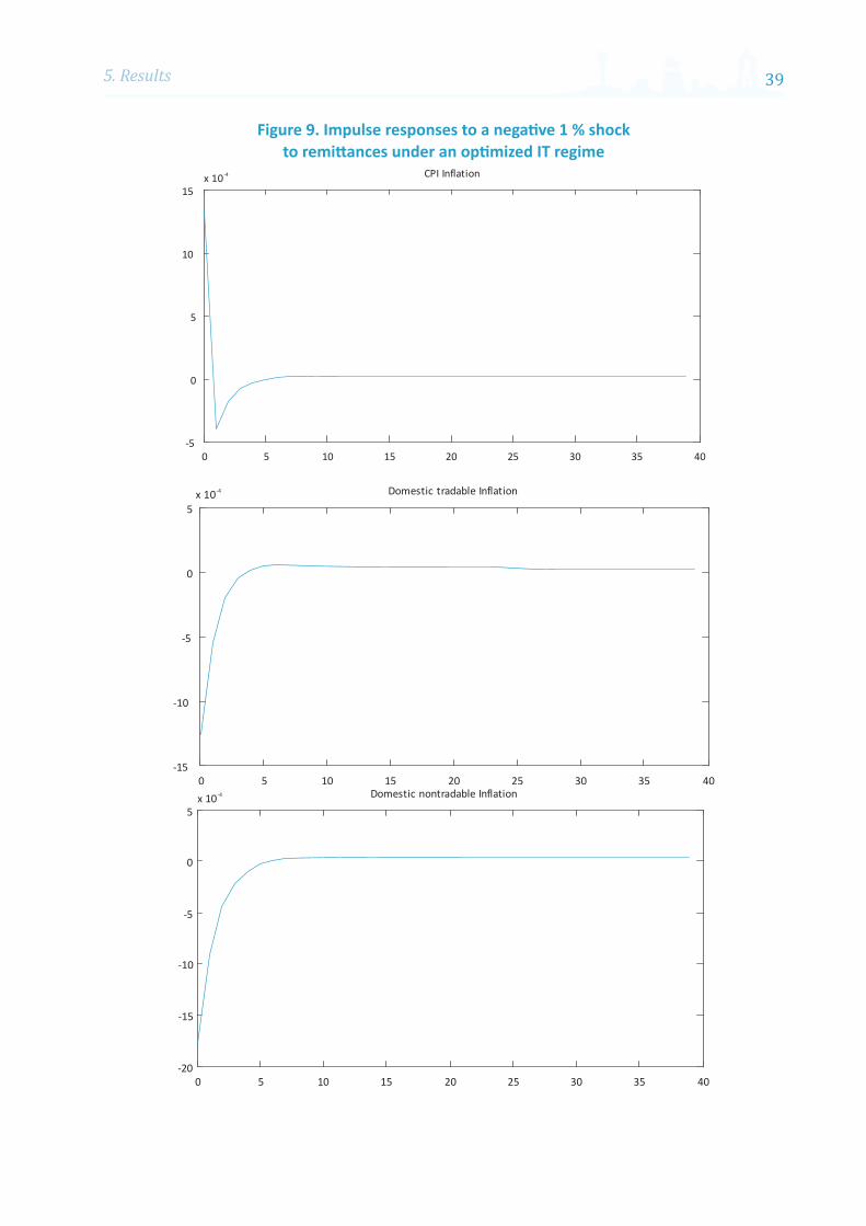
395. Results
Figure 9. Impulse responses to a negative 1 % shock to remittances under an optimized IT regime

On the Possibility of Inflation Targeting in Kyrgyzstan40

415. Results
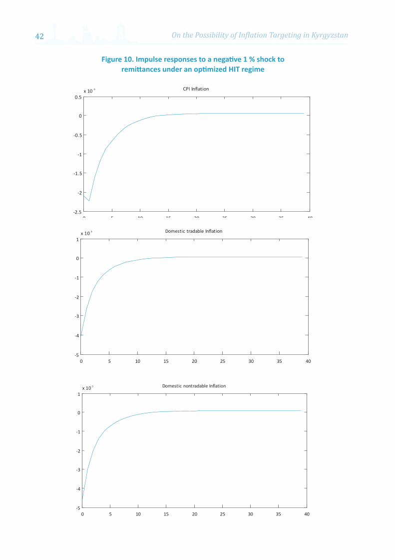
On the Possibility of Inflation Targeting in Kyrgyzstan42
Figure 10. Impulse responses to a negative 1 % shock to remittances under an optimized HIT regime

435. Results

On the Possibility of Inflation Targeting in Kyrgyzstan44

455. Results
However, it should be stressed that the result that exchange rate management entails losses is true if the exchange rate is already relatively close to its longrun equilibrium, which is not the case in KR. Moreover, the model does not (explicitly) take into account “fear of floating” considerations and high currency substitution/dollarization in the country. These would naturally require some (minor) foreign exchange interventions on the CB’s side. The costs of such interventions are almost negligible but they will help to stabilize excessive exchange rate fluctuations. To sum up, it is desirable that the NBKR targets inflation aggressively and at the same time does some minor interventions to stabilize the exchange rate. In other words, some form of HIT regime (which does not require that all the preconditions for FFIT are met), with aggressive control over inflation, would be most appropriate for the country at its current stage of development.
Sensitivity analysis
The case of more flexible tradable sector
We also conducted policy experiments with lower price stickiness in the tradable sector, which is deemed to be more a plausible specification. We set this parameter equal to 1/3 for the tradable sector and recalculated conditional welfare for each monetary arrangement. As in the case with the same degree of stickiness in tradable and non-tradable sectors (θ = 2/3), the lowest welfare loss, under both IT and HIT regimes, is achieved when the inflation policy reaction parameter takes the highest value in the grid, Ωπ = 3. Furthermore, IT continues to outperform other arrangements. The optimised fiscal policy reaction coefficient under all three monetary arrangements, Ω1, remains the same as before. However, the welfare losses (relative to steady state) under optimised policy combinations in the case with different price stickiness across sectors are now slightly lower relative to that under the same degree of price rigidity. For instance, if the welfare loss of optimised IT and consumption tax in the case of the same price stickiness was 0.49 % of steady state consumption equivalent, then in the case of a more flexible tradable sector, the welfare loss is 0.46 %. This is the result that one would expect; the decrease in the extent of distortions caused by price rigidities leads to lower welfare losses. The same result holds true for all the optimized monetary and fiscal policy combinations.
No shocks to remittances
In the previous subsection, we argued that it appears that welfare benefits of lower inflation volatility outweigh the benefits of lower exchange rate volatility. As the next experiment, we examined whether the IT framework remains desirable when some of the features specific to the Kyrgyz economy are shut down. In particular, we recalculated optimised welfare outcomes under alternative policy combinations when consumers do not face remittances shocks.61 In this exercise, we also allowed for a lower degree of price stickiness in the tradable sector. As before, IT outperformed the other monetary regimes. The minimum welfare loss across alternative policy combinations occurs when the CB targets inflation aggressively under both IT and HIT frameworks, for example, Ωπ = 3. The optimised fiscal policy coefficients remain the same as before (reported in Table 5).
61 In this experiment, we did not exclude remittances from the model. Rather, we treated remittances as a constant. In this case, they can be viewed as some kind of fixed amount subsidies provided by a third party to the households.

On the Possibility of Inflation Targeting in Kyrgyzstan46
6. Conclusions and policy implications
This paper has examined whether or not the KR meets the commonly accepted prerequisites for the successful adoption of IT regime, and whether it is worthwhile for the country to adopt an IT regime. We conclude that the country is not meeting most of the commonly accepted preconditions for the successful adoption of the FFIT in view of: de facto lack of CB independence and credibility (and absence of accountability), weak monetary transmission mechanisms, high degree of dollarization, large informal sector, underdeveloped financial market, high vulnerability to external shocks, and the limited technical capacity of the NBKR. Therefore, it is premature for the country to switch to FFIT regime. However, as experiences in other countries show, many successful IT-implementing countries had not met most of the required preconditions prior to the adoption of an IT framework. They adopted some milder forms of IT regime, similar to what Armenia and Georgia did, and then gradually switched to full-fledgedIT regime.
We also built and solved a small open economy model calibrated for the KR and studied welfare implications of alternative monetary regimes that may be followed by the NBKR: IT, HIT and fixed exchange rate regime. The results suggest that the economy could benefit if the NBKR targets inflation aggressively and, at the same time, intervenes on foreign exchange markets moderately to smooth out excessive exchange rate fluctuations. Therefore, adopting some form of a HIT regime could be an option for the country. Apart from the benefits discussed above, adoption of a HIT framework could also contribute to increasing accountability and improving the credibility of the NBKR.

47Annexes
Annexes
Annex A
A.1 Variables written in real terms
This annex presents the set of equations consisting of first order and equilibrium conditions written in real terms. Let us rewrite nominal variables in real terms and introduce some new variables: mt = Mt / Pt , bH,t = BH,t / Pt , dt = et BF,t / Pt.
Scaled internal price ratio:,
,
N tt
H t
PQ
P=
Scaled terms of trade:,
,
F tt
H t
PS
P=
Using definitions of price indexes, one can get the following identities that will be useful later:
, 1 ( 1)(1 )N tt t
t
PQ S
Pγ ε γ− − −=
, ( 1)(1 )H tt t
t
PQ S
Pγ ε γ− − −=
, (1 )F tt t
t
PQ S
Pγ ε γ γ− − +=
A.2 Equilibrium conditions in real variables
This section presents equilibrium and first order conditions written in real terms.
1 1,
1 1
1 1 (1 ) 1 1
ct t t
t f tct t t t
C eE iC e
ρτβτ π
−
+ +
+ +
+ + = +
(A.1)
1
1 1
1 1 (1 ) 1 1
ct t
t tct t t
CE iC
ρτβτ π
−
+
+ +
+ + = +
(A.2)
1 01
lt
t t tct
C Hρ ψτωτ
− −− =
+ (A.3)
mt = νwt Ht (A.4)
Ht = HH,t + HN,t (A.5)
, 1, , ,
(1 )1t
tt
tN t
N t N t N t
iw Pimc
A H Pα
ν
α −
++
=
(A.6)
YN,t = AN,t H αN,t / sN,t (A.7)

On the Possibility of Inflation Targeting in Kyrgyzstan48
1,
, ,N t
N t t N tt
Pa Y Y
Pγ
−
= =
(A.8)
1
,1 1 1, , , , 1 1
, 1, 1
ˆ 1ˆˆ
N tt N t N t N t t t t t
N tN t
Px P a mc E x
P
ω
ω θ σπ
− −
− −+ +
++
= +
(A.9)
,2 2, , , 1 1
, 1, 1
ˆ 1ˆˆ
N tt N t N t t t t t
N tN t
Px P a E x
P
ω
ω θ σπ
−
−+ +
++
= +
(A.10)
1 2
1t tx xωω
=−
(A.11)
θπ ω N –,
1t + (1 – θ) P
∼∧ 1 N
–,
ωt = 1 (A.12)
sN,t = (1 – θ) P∼∧ –ω + θπ ω N,t sN,t–1 (A.13)
, 1, , ,
(1 )1t
tt
tH t
H t H t H t
iw Pimc
A H Pα
ν
α −
++
=
(A.14)
1
,* *, , , ,
,
/H tH t t H t H t H t
F t
PY Y A H s
Pαε
−
+ =
(A.15)
11 1 1, , , ,* * * *
, *,
(1 ) H t H t H t H tH t t t t t
t t t t F t
P P P Pa Y Y Y Y
P e P P Pε γ ε ε
−− − − = − + = +
(A.16)
1
,3 1 3, , , , 1 1
, 1, 1
ˆ 1ˆˆ
H tt H t H t H t t t t t
H tH t
Px P a mc E x
P
η
η θ σπ
− −
− −+ +
++
= +
(A.17)
,4 4, , , 1 1
, 1, 1
ˆ 1ˆˆ
H tt H t H t t t t t
H tH t
Px P a E x
P
η
η θ σπ
−
−+ +
++
= +
(A.18)
3 4
1t tx xωω
=−
(A.19)
θπ η H
–,
1t + (1 – θ) P
∼∧ 1 H
–,
ηt = 1 (A.20)
sH,t = (1 – θ) P∼∧ –η + θπ η
H,t sH,t–1 (A.21)
*
1 1 ,
t t t
t t H t
S eS e
ππ− −
=
(A.22)
,
1 ,
N tt
t H t
ππ−
=
(A.23)
πt = π γN,t π ε H,
( 1t–γ) π t
*(1– ε)(1–γ) (et / et–1 )
(1– ε)(1–γ) (A.24)

49Annexes
Yt = Ct + Gt (A.25),*
, 1 1 ,1
1(1 ) H tt tt F t t H t t t
t t t t
Pe TRd i d C e Ye P Pπ− −−
= + − − + (A.26)
1 1 11 1(1 )c l
t t t t t t t t t t tt t
m b C H i b m Gτ τ ωπ π− − −+ + + = + + +
(A.27),
,F t
t t F tt
PGDP Y Y
P= −
(A.28)τt = τ ct Ct + τ lt wt Ht (A.29)
1 1 1 11( ) /j j
t t t t t t tt
G i b GDP GDPτ τ τ κπ− −= +Ω − + − , j=c, l (A.30)
ln((1 + it ) / (1 + i–)) = λ ln((1 + it–1 ) / (1 + i–)) + (1 – λ) [Ωπ ln(πt / π–) + Ωe ln(et / e
–)] (A.31)
ln(Gt / G–) = ρg ln(Gt–1 / G
–) + eg,t (A.32)
ln(π*t / π
–*) = ρπ ln(π*t–1 / π
–*) + επ (A.33)
ln(Y *t / Y–*) = ρY ln(Y *t–1 / Y
–*) + εY (A.34)
ln((1 + i*t ) / (1 + i–*)) = ρI ln((1 + i*
t–1 ) / (1 + i–*)) + εi (A.35)
ln(Aj,t / Aj ) = φln(Aj,t–1 / Aj ) + ςj,t , j=H, N (A.36)
ln(TRt / TR ) = ρtr ln(TRt–1 / TR ) + εtr,t (A.37)
A.3 Model equations, states and controls
The system is given by: consumption Euler equations (A.1) and (A.2), CIA constraint (A.4), domestic non-tradable intermediate goods market clearing condition (A.7), domestic non-tradable sector price setting equations (A.9) and (A.10), law of motion for domestic non-tradable price dispersion (A.13), domestic tradable goods market clearing condition (A.15), domestic tradable sector price setting equations (A.17) and (A.18), law of motion for domestic tradable price dispersion (A.21), laws of motion for scaled terms of trade and scaled internal price ratio (A.22) and (A.23), law of motion for CPI inflation (A.24), foreign debt accumulation equation (A.26), government budget constraint (A.27), money rule (A.31), exogenous stochastic processes (A.32-37), and a fiscal rule equation (A.30). There are 24 first order difference equations describing equilibrium and first order conditions. In addition, there are two auxiliary equations linking previous period nominal exchange rate and domestic interest rate on bond holdings to the current period, since we have these variables entering the system with t-1, t and t+1 time subscripts. We also have one intertemporal welfare deviation measure that would make the calculation of welfare loss possible.

On the Possibility of Inflation Targeting in Kyrgyzstan50
We have used the following intratemporal conditions to make additional simplifications to reduce the number of equations: (A.8) to substitute domestic demand for domestically produced non-tradable goods; (A.6) and (A.3) to substitute for non-tradable marginal cost and real wage; (A.11) to substitute out x 2t ; (A.12) to express the relative price of the non-tradable intermediate good as a function of non-tradable price inflation; (A.14) to substitute for marginal costs in the tradable sector; (A.16) to substitute for the domestically-produced tradable intermediate good; (A.19) to substitute out x 4t ; (A.20) to substitute for the relative price in the tradable sector; (A.25) to express the final good as a function of private and public consumption; (A.28) for the definition of GDP.
All together, we have 28 first order difference equations in 28 variables. The next step is to split the variables into controls and states. The state variables are collected in x:
endogt
t exogt
xx
x
=
, where x tendog is a vector of endogenous state variables, and x t
exog is a vector of
exogenous state variables.
x tendog = [ et–1 St–1 Qt–1 it–1 mt–1 bt–1 sN,t–1 sH,t–1 dt–1 ]´.
x texog = [ Y *t–1 π
*t–1 Gt–1 AN,t AH,t i
*t–1 ]´.
The vector of controls, y, is given by: yt = [ Ct Ht HN,t it πt πH,t πN,t it et x 1t x 3t τ jt ]´, j=c,l depending
on which tax instrument is used.

51Figures
3
2.9
2.8
2.7
2.6
2.5
2.4
2.3
2.2
2.1
21.
91.
81.
71.
61.
51.
41.
31.
21.
11
0.9
0.8
0.7
0.6
0.5
0.4
0.3
0.2
0.1
3*
**
**
**
**
**
**
**
**
**
**
**
**
**
**
*
2.9
**
**
**
**
**
**
**
**
**
**
**
**
**
**
**
2.8
**
**
**
**
**
**
**
**
**
**
**
**
**
**
**
2.7
**
**
**
**
**
**
**
**
**
**
**
**
**
**
**
2.6
**
**
**
**
**
**
**
**
**
**
**
**
**
**
**
2.5
**
**
**
**
**
**
**
**
**
**
**
**
**
**
**
2.4
**
**
**
**
**
**
**
**
**
**
**
**
**
**
**
2.3
**
**
**
**
**
**
**
**
**
**
**
**
**
**
**
2.2
**
**
**
**
**
**
**
**
**
**
**
**
**
**
**
2.1
**
**
**
**
**
**
**
**
**
**
**
**
**
**
**
2*
**
**
**
**
**
**
**
**
**
**
**
**
**
**
*
1.9
**
**
**
**
**
**
**
**
**
**
**
**
**
**
**
1.8
**
**
**
**
**
**
**
**
**
**
**
**
**
**
**
1.7
**
**
**
**
**
**
**
**
**
**
**
**
**
**
**
1.6
**
**
**
**
**
**
**
**
**
**
**
**
**
**
**
1.5
**
**
**
**
**
**
**
**
**
**
**
**
**
**
**
1.4
. .
. .
. .
. .
. .
. .
. .
. .
. .
. .
. .
. .
. .
. .
. .
1.3
. .
. .
. .
. .
. .
. .
. .
. .
. .
. .
. .
. .
. .
. .
. .
1.2
. .
. .
. .
. .
. .
. .
. .
. .
. .
. .
. .
. .
. .
. .
. .
1.1
. .
. .
. .
. .
. .
. .
. .
. .
. .
. .
. .
. .
. .
. .
. .
1 .
. .
. .
. .
. .
. .
. .
. .
. .
. .
. .
. .
. .
. .
. .
.
0.9
. .
. .
. .
. .
. .
. .
. .
. .
. .
. .
. .
. .
. .
. .
. .
0.8
. .
. .
. .
. .
. .
. .
. .
. .
. .
. .
. .
. .
. .
. .
. .
0.7
. .
. .
. .
. .
. .
. .
. .
. .
. .
. .
. .
. .
. .
. .
. .
0.6
. .
. .
. .
. .
. .
. .
. .
. .
. .
. .
. .
. .
. .
. .
. .
0.5
. .
. .
. .
. .
. .
. .
. .
. .
. .
. .
. .
. .
. .
. .
. .
0.4
. .
. .
. .
. .
. .
. .
. .
. .
. .
. .
. .
. .
. .
. .
. .
0.3
. .
. .
. .
. .
. .
. .
. .
. .
. .
. .
. .
. .
. .
. .
. .
0.2
. .
. .
. .
. .
. .
. .
. .
. .
. .
. .
. .
. .
. .
. .
. .
0.1
. .
. .
. .
. .
. .
. .
. .
. .
. .
. .
. .
. .
. .
. .
. .
Appe
ndix
BFi
gure
B1.
Det
erm
inac
y re
gion
s un
der
IT a
nd D
efic
it R
ule
: Con
sum
ptio
n ta
x.
A s
tar
corr
espo
nds
to u
niqu
e eq
uilib
rium
, a d
ot d
enot
es a
n ex
plos
ive
solu
tion
.
πΩ
1Ω

On the Possibility of Inflation Targeting in Kyrgyzstan52Fi
gure
B2.
Det
erm
inac
y re
gion
s un
der
IT a
nd D
efic
it R
ule:
Lab
our
tax.
A
sta
r co
rres
pond
s to
uni
que
equi
libri
um, a
dot
den
otes
an
expl
osiv
e so
luti
on.
πΩ
1Ω
3
2.9
2.8
2.7
2.6
2.5
2.4
2.3
2.2
2.1
21.
91.
81.
71.
61.
51.
41.
31.
21.
11
0.9
0.8
0.7
0.6
0.5
0.4
0.3
0.2
0.1
3*
**
**
**
**
**
**
**
**
**
**
**
**
**
**
*
2.9
**
**
**
**
**
**
**
**
**
**
**
**
**
**
**
2.8
**
**
**
**
**
**
**
**
**
**
**
**
**
**
**
2.7
**
**
**
**
**
**
**
**
**
**
**
**
**
**
**
2.6
**
**
**
**
**
**
**
**
**
**
**
**
**
**
**
2.5
**
**
**
**
**
**
**
**
**
**
**
**
**
**
**
2.4
**
**
**
**
**
**
**
**
**
**
**
**
**
**
**
2.3
**
**
**
**
**
**
**
**
**
**
**
**
**
**
**
2.2
**
**
**
**
**
**
**
**
**
**
**
**
**
**
**
2.1
**
**
**
**
**
**
**
**
**
**
**
**
**
**
**
2*
**
**
**
**
**
**
**
**
**
**
**
**
**
**
*
1.9
**
**
**
**
**
**
**
**
**
**
**
**
**
**
**
1.8
**
**
**
**
**
**
**
**
**
**
**
**
**
**
**
1.7
**
**
**
**
**
**
**
**
**
**
**
**
**
**
**
1.6
**
**
**
**
**
**
**
**
**
**
**
**
**
**
**
1.5
**
**
**
**
**
**
**
**
**
**
**
**
**
**
**
1.4
**
**
**
**
**
**
**
**
**
**
**
**
**
**
**
1.3
**
**
**
**
**
**
**
**
**
**
**
**
**
**
**
1.2
**
**
**
**
**
**
**
**
**
**
**
**
**
**
**
1.1
..
..
..
..
..
..
..
..
..
..
..
..
..
..
..
1.
..
..
..
..
..
..
..
..
..
..
..
..
..
..
.
0.9
..
..
..
..
..
..
..
..
..
..
..
..
..
..
..
0.8
..
..
..
..
..
..
..
..
..
..
..
..
..
..
..
0.7
..
..
..
..
..
..
..
..
..
..
..
..
..
..
..
0.6
..
..
..
..
..
..
..
..
..
..
..
..
..
..
..
0.5
..
..
..
..
..
..
..
..
..
..
..
..
..
..
..
0.4
..
..
..
..
..
..
..
..
..
..
..
..
..
..
..
0.3
..
..
..
..
..
..
..
..
..
..
..
..
..
..
..
0.2
..
..
..
..
..
..
..
..
..
..
..
..
..
..
..
0.1
..
..
..
..
..
..
..
..
..
..
..
..
..
..
..

53FiguresFi
gure
B3.
Det
erm
inac
y re
gion
s un
der
HIT
and
Def
icit
Rul
e: C
onsu
mpt
ion
tax.
A
sta
r co
rres
pond
s to
uni
que
equi
libri
um, a
dot
den
otes
an
expl
osiv
e so
luti
on.
πΩ
1Ω
3
2.9
2.8
2.7
2.6
2.5
2.4
2.3
2.2
2.1
21.
91.
81.
71.
61.
51.
41.
31.
21.
11
0.9
0.8
0.7
0.6
0.5
0.4
0.3
0.2
0.1
3*
**
**
**
**
**
**
**
**
**
**
**
**
**
**
*
2.9
**
**
**
**
**
**
**
**
**
**
**
**
**
**
**
2.8
**
**
**
**
**
**
**
**
**
**
**
**
**
**
**
2.7
**
**
**
**
**
**
**
**
**
**
**
**
**
**
**
2.6
**
**
**
**
**
**
**
**
**
**
**
**
**
**
**
2.5
**
**
**
**
**
**
**
**
**
**
**
**
**
**
**
2.4
**
**
**
**
**
**
**
**
**
**
**
**
**
**
**
2.3
**
**
**
**
**
**
**
**
**
**
**
**
**
**
**
2.2
**
**
**
**
**
**
**
**
**
**
**
**
**
**
**
2.1
**
**
**
**
**
**
**
**
**
**
**
**
**
**
**
2*
**
**
**
**
**
**
**
**
**
**
**
**
**
**
*
1.9
**
**
**
**
**
**
**
**
**
**
**
**
**
**
**
1.8
**
**
**
**
**
**
**
**
**
**
**
**
**
**
**
1.7
**
**
**
**
**
**
**
**
**
**
**
**
**
**
**
1.6
**
**
**
**
**
**
**
**
**
**
**
**
**
**
**
1.5
**
**
**
**
**
**
**
**
**
**
**
**
**
**
**
1.4
..
..
..
..
..
..
..
..
..
..
..
..
..
..
..
1.3
..
..
..
..
..
..
..
..
..
..
..
..
..
..
..
1.2
..
..
..
..
..
..
..
..
..
..
..
..
..
..
..
1.1
..
..
..
..
..
..
..
..
..
..
..
..
..
..
..
1.
..
..
..
..
..
..
..
..
..
..
..
..
..
..
.
0.9
..
..
..
..
..
..
..
..
..
..
..
..
..
..
..
0.8
..
..
..
..
..
..
..
..
..
..
..
..
..
..
..
0.7
..
..
..
..
..
..
..
..
..
..
..
..
..
..
..
0.6
..
..
..
..
..
..
..
..
..
..
..
..
..
..
..
0.5
..
..
..
..
..
..
..
..
..
..
..
..
..
..
..
0.4
..
..
..
..
..
..
..
..
..
..
..
..
..
..
..
0.3
..
..
..
..
..
..
..
..
..
..
..
..
..
..
..
0.2
..
..
..
..
..
..
..
..
..
..
..
..
..
..
..
0.1
..
..
..
..
..
..
..
..
..
..
..
..
..
..
..

On the Possibility of Inflation Targeting in Kyrgyzstan54Fi
gure
B4.
Det
erm
inac
y re
gion
s un
der
HIT
and
Def
icit
Rul
e: L
abou
r ta
x.
A s
tar
corr
espo
nds
to u
niqu
e eq
uilib
rium
, a d
ot d
enot
es a
n ex
plos
ive
solu
tion
.
πΩ
1Ω
3
2.9
2.8
2.7
2.6
2.5
2.4
2.3
2.2
2.1
21.
91.
81.
71.
61.
51.
41.
31.
21.
11
0.9
0.8
0.7
0.6
0.5
0.4
0.3
0.2
0.1
3*
**
**
**
**
**
**
**
**
**
**
**
**
**
**
*
2.9
**
**
**
**
**
**
**
**
**
**
**
**
**
**
**
2.8
**
**
**
**
**
**
**
**
**
**
**
**
**
**
**
2.7
**
**
**
**
**
**
**
**
**
**
**
**
**
**
**
2.6
**
**
**
**
**
**
**
**
**
**
**
**
**
**
**
2.5
**
**
**
**
**
**
**
**
**
**
**
**
**
**
**
2.4
**
**
**
**
**
**
**
**
**
**
**
**
**
**
**
2.3
**
**
**
**
**
**
**
**
**
**
**
**
**
**
**
2.2
**
**
**
**
**
**
**
**
**
**
**
**
**
**
**
2.1
**
**
**
**
**
**
**
**
**
**
**
**
**
**
**
2*
**
**
**
**
**
**
**
**
**
**
**
**
**
**
*
1.9
**
**
**
**
**
**
**
**
**
**
**
**
**
**
**
1.8
**
**
**
**
**
**
**
**
**
**
**
**
**
**
**
1.7
**
**
**
**
**
**
**
**
**
**
**
**
**
**
**
1.6
**
**
**
**
**
**
**
**
**
**
**
**
**
**
**
1.5
**
**
**
**
**
**
**
**
**
**
**
**
**
**
**
1.4
**
**
**
**
**
**
**
**
**
**
**
**
**
**
**
1.3
**
**
**
**
**
**
**
**
**
**
**
**
**
**
**
1.2
**
**
**
**
**
**
**
**
**
**
**
**
**
**
**
1.1
..
..
..
..
..
..
..
..
..
..
..
..
..
..
..
1.
..
..
..
..
..
..
..
..
..
..
..
..
..
..
.
0.9
..
..
..
..
..
..
..
..
..
..
..
..
..
..
..
0.8
..
..
..
..
..
..
..
..
..
..
..
..
..
..
..
0.7
..
..
..
..
..
..
..
..
..
..
..
..
..
..
..
0.6
..
..
..
..
..
..
..
..
..
..
..
..
..
..
..
0.5
..
..
..
..
..
..
..
..
..
..
..
..
..
..
..
0.4
..
..
..
..
..
..
..
..
..
..
..
..
..
..
..
0.3
..
..
..
..
..
..
..
..
..
..
..
..
..
..
..
0.2
..
..
..
..
..
..
..
..
..
..
..
..
..
..
..
0.1
..
..
..
..
..
..
..
..
..
..
..
..
..
..
..

55Figures
References
Ali Al-Eyd, David Amaglobeli, Bahrom Shukurov, and Mariusz. Sumlinski. , “Global Food Price Inflation and Policy Responses in Central Asia.” International Monetary Fund (IMF) Working Paper No. 86. Washington DC: IMF, March 2012.
King Banaian, David Kemme and Grigor Sargsyan. “Inflation Targeting in Armenia: Monetary Policy in Transition.” Comparative Economic Studies, vol. 50, no. 3. September2008.
Nicoletta Batini and Douglas Laxton. “Under What Conditions Can Inflation Targeting be Adopted? The Experience of Emerging Markets” in Monetary Policy Under Inflation Targeting ed. Frederic S. Mishkin and Klaus Schmidt-Hebel Santiago: Banco Central de Chile, 2005.
Guillermo Calvo. ”Staggered Prices in a Utility-Maximizing Framework.” Journal of Monetary Economics no. 12, 1983: 383-398.
Guillermo Calvo and Carmen M. Reinhart. “Fear of Floating.” National Bureau of Economic Research (NBER) Working Paper 7993. Cambridge: NBER, 2000.
Luis Felipe Céspedes, RobertoChang and Andres Velasco, “Balance Sheets and Exchange Rate Policy,” American Economic Review no. 94. September 2004: 1183–1193.
Lawrence Christiano, Martin Eichenbaum, and Charles Evans. “Sticky Price And Limited Participation Models Of Money: A Comparison,” European Economic Review, vol. 41(6), June 1997: 1201-1249.
Christopher W. Crowe and Ellen E Meade, “Central Bank Independence and Transparency: Evolution and Effectiveness,” International Monetary Fund (IMF) Working Paper No. 08/119, (Washington DC: IMF, 2008.)
Alex Cukierman. Central Bank Strategy, Credibility and Independence: Theory and Evidence. Cambridge, MA: MIT Press, 1992.
Era Dabla-Norris, Daehaeng Kim, Mayra Zermeño,. Andreas Billmeier, and Vitali Kramarenko. , “Modalities of Moving to Inflation Targeting in Armenia and Georgia.” International Monetary Fund (IMF) Working Paper No. 133. Washington DC: IMF, 2007.
Sebatian Edwards and Miguel Savastano. “Exchange Rates in Emerging Economies: What Do We Know? What Do We Need to Know?” National Bureau of Economic Research (NBER) Working Paper 7228. Cambridge: NBER, 1999.
Barry Eichengreen, Paul. Masson, Miguel Savastano, and Sunil Sharma. “Transition Strategies and Nominal Anchors on the Road to Greater Exchange Rate Flexibility.” Essays in International Economics. Princeton, N.J.: Princeton University, 1999.
Arminio Fraga, Ilan Goldfajn and Andre Minella. “Inflation Targeting in Emerging Market Economies.” National Bureau of Economic Research (NBER) Working Paper 10019. Cambridge: NBER, 2003.
On the Possibility of Inflation Targeting in Kyrgyzstan56
Benjamin Friedman and Kenneth Kuttner. “A Price Target for U.S. Monetary Policy? Lessons from the Experience with Money Growth Targets.” Brookings Papers on Economic Activity, no 1. Washington DC: The Brookings Institution, 1996.
Jordi Gali and Tomasso Monacelli. “Monetary Policy and Exchange Rate Volatility in a Small Open Economy.” Review of Economic Studies no. 72, 2005: 707-734.
Mark Gertler, Simon Gilchrist and Fabio Natalucci. “External Constraints on Monetary Policy and the Financial Accelerator,” National Bureau of Economic Research (NBER) Working Paper 10128. Cambridge: NBER, 2003.
Geoffrey Heenan, Marcel Peter, and Scott Roger. “Implementing Inflation Targeting: Institutional Arrangements, Target Design, and Communication.” International Monetary Fund Working Paper 06/278. Washington DC: IMF, 2006.
International Monetary Fund (IMF). IMF Country Report No. 09/209. Washington DC: IMF, 2009.
_____. IMF Country Report No. 11/354. Washington DC: IMF, 2011.
Nurbek Jenish, “Choice of Exchange Rate Regime for Partially Dollarized Developing Economies,” Central European University Working Paper (2008a.).
_____. “Optimal Monetary and Fiscal Policy Rules for New European Union (EU) Countries on Their Road to Euro,” Central European University Working Paper (2008b).
Paul Masson, Miguel Savastano and Sunil Sharma. “Can Inflation Targeting be a Framework for Monetary Policy in Developing Countries?” Finance and Development. Washington DC: International Monetary Fund, March, 1998: 34-38.
Frederic S. Mishkin. “Inflation Targeting in Emerging Market Countries.” American Economic Review, vol. 85, no.2, May 2000.
_____. “Monetary Policy.” National Bureau of Economic Research (NBER) Reporter Winter 2001/2.
_____. “Can Inflation Targeting Work in Emerging Market Countries?” National Bureau of Economic Research (NBER) Working Paper 10646. Cambridge: NBER, July 2004.
Frederic S. Mishkin and Miguel Savastano, 2002. “Monetary Policy Strategies for Emerging Market Countries: Lessons from Latin America,” Comparative Economic Studies, Vol. 54, No. 2,
pp. 45-82.
Tomasso Monacelli. “Monetary Policy in a Low Pass-Through Environment.” Journal of Money Credit and Banking, vol. 37 no. 6, 2005: 1047-1066.
Fabio Massimo Natalucci and Federico Ravenna. “Monetary Policy Choices in Emerging Market Economies: the Case of High Productivity Growth,” Journal of Money, Credit and Banking, forthcoming.

57Figures
Maurice Obstfeld and Kenneth Rogoff. “The Mirage of Fixed Exchange Rates,” Journal of Economic Perspectives no. 9 vol. 4, 1995: 73-96.
Scott Roger. “Inflation Targeting Turns 20.” Finance and Development, vol. 47 no. 1. Washington DC: International Monetary Fund, March 2010.
Stephanie Schmitt-Grohé and Martín Uribe. “Closing Small Open Economy Models.” Journal of International Economics, vol. 61(1), (2003): 163-185.
Stephanie Schmitt-Grohé and Martín Uribe “Solving Dynamic General Equilibrium Models Using Second Order Approximation to the Policy Function.” Journal of Economic Dynamics and Control no. 28, 2004: 755-775.
_____. “Optimal Simple and Implementable Monetary and Fiscal Rules.” Journal of Monetary Economics no, 54, 2007.
Michael Woodford. “Monetary Policy and Price-Level Determinacy in a Cash-in-Advance Economy,” Economic Theory no. 4, (1994): 345-380.
_____. “Price-level Determinacy without Control of a Monetary Aggregate,” Carnegie-Rochester Conference Series on Public Policy no. 43, (1995): 1-46.
_____. “Control of the Public Debt: A Requirement for Price Stability?” National Bureau of Economic Research (NBER) Working Paper 5684. (Cambridge: NBER, 1996).
_____. “Public Debt and the Price Level,” Working Paper, (Princeton: Princeton University, 1998.)
_____. “Fiscal Requirements for Price Stability,” Journal of Money Credit and Banking no. 33, (2001): 669-728.Tak Yun, “Nominal Price Rigidity, Money Supply Endogeneity, and Business Cycles,” Journal of Monetary
Economics no. 37, (1996): 345-370.

On the Possibility of Inflation Targeting in Kyrgyzstan58
For Notes

59For Notes

On the Possibility of Inflation Targeting in Kyrgyzstan60
Produced by UCA Communications DepartmentCopy edited by Sia Nowrojee
Printed by VRS, Bishkek, Kyrgyz Republic


www.ucentralasia.org