ON THE PRICING OF CORPORATE DEBT:

THE RISK STRUCTURE OF INTEREST RATES*

by

Robert C. Merton

684-73

November 1973

To be presented at the American Finance Association Meetings, New York,December 1973."

ON THE PRICING OF CORPORATE DEBT: THE RISK STRUCTURE OF INTEREST PATES

Robert C. Merton

I. Introduction

The value of a particular issue of corporate debt depends esentially

on three items: (1) the required rate of return on riskless (in terms of

default) debt (e.&., government bonds or very high-grade corporate bonds);

(2) the various provisions and restrictions contained in the indenture (e.g.,

maturity date, coupon rate, call terms, seniority in the event of default,

sinking fund, etc.); (3) the probability that the firm will be unable to

satisfy some or all of the indenture requiremerits (i.e., the probability of

default).

While a number of theories and empirical studies has been published

on the term structure of interest rates (item 1), there has been no systematic

development of a theory for pricing bonds when there is a significant proba-

bility of default. The purpose of this paper is to present such a theory

which might be called a theory of the risk structure of interest rates. Te

use of the term "risk" is restricted to the possible gains or losses to bond-

holders as a result of (unanticipated) changes in the probability of default

and does not include the gains or losses inherent to all bonds caused by

(unanticipated) changed in interest rates in general. Throughout most of

the analysis, a given term structure is assumed and hence, the price differ-

entials among bonas will be solely caused by differences in the probability

of default.

-2-

In a seminal paper, Black and Scholes [1] present a complete

general equilibrium theory of option pricing which is particularly attract-

ive because the final formula is a function of "observable" variables.

Therefore, the model is subject to direct empirical tests which they [21

performed with some success. Merton [5] clarified and extended the Black-

Scholes model. While options are highly specialized and relatively unim-

portant financial instruments, both Black and Scholes [1] and Merton [5, 6]

recognized that the same basic approach could be applied in developing a

pricing theory for corporate liabilities in general.

In Section II of the paper, the basic equation for the pricing

of financial instruments is developed along Black-Scholes lines. In

Section III, the model is applied to the simplest form of corporate debt,

the discount bond where no coupon payments are made, and a formula for com-

puting the risk structure of interest rates is presented. In Section IV, com-

parative statics are used to develop graphs of the risk structure, and the

question of whether the term premium is an adequate measure of the risk of

a bond is answered. In Section V, the validity in the presence of bank-

ruptcy of the famous Modigliani-Miller theorem [7] is proven, and the re-

quired return on debt as a function of the debt-to-equity ratio is deduced.

In Section VI, the analysis is extended to include coupon and callable

bonds.

-.___ __CI-__- -- ----- 1111 ~ ~1~

-3-

II. On the Pricing of Corporate Liabilities

To develop the Black-Scholes-type pricing model, we make the

owing assumptions:

A.1 there are no transactions costs, taxes, or problems with indivis-

ibilities of assets.

A.2 there are a sufficient number of investors with comparable wealth

levels so that each investor believes that he can buy and sell as

much of an asset as he wants at the market price.

A.3 there exists an exchange market for borrowing and lending at the

same rate of interest.

A.4 short-sales of all assets, with full use of the proceeds, is allowE

A.5 trading in assets takes place continuously in tme.

A.6 the Modigliani-Miller theorem that the value of the firm is

invariant to its capital structure obtains.

A.7 the Term-Structure is "flat" and known with certainty. I.e., the

price of a riskless discount bond which promises a payment of one

dollar at time T in the future is P(T) = exp[-rT] where r is the

(instantaneous) riskless rate of interest, the same for all time.

A.8 The dynamics for the value of the firm, V, through time can be

described by a diffusion-type stochastic process with stochastic

differential equation

Ed.

dV = (aV - C) dt + aVdz

where

a is the instantaneous expected rate of return on the firm per unit

time, C is the total dollar payouts by the firm per unit time to

follC

-4-

either its shareholders or liabilities-holders (e.g., dividends

or interest payments) if positive, ana it is the net dollars

received by the firm from new financing if negative; 2 is the

instantaneous variance of the return cn the firm per unit time;

dz is a standard Gauss-Wiener process.

Many of these assumptions are not necessary for the model to obtain but are

chosen for expositional convenience. In particular, the "perfect market"

assumptions (A.1 -A.4) can be substantially weakened. A.6 is actually proved

as part or the analysis and A.7 is chosen so as to clearly distinguish risk

structure rrom term structure effects on pricing. A.5 and A.8 are the critical

assumptions. Basically, A.5 requires Lhat the market for these securities

is open for trading most of time. A.8 requires that price movements

are continuous and that the unanticipated) returns on the securities be

serially independent which is consistent with the "efficient markets hypothesis"

of Fama [ 3] and Samuelson [ 9 1/

Suppose there exists a security whose market value, Y, at any point in

time can be written as a function of the value of the firm and time, i.e.,

Y = F(V,t). We can formally write the dynamics of this security's value

in stochastic differential equation form as

dY = [a Y - C dt + Ydz (1)Y Y Y Y

where

oa is the instantaneous expected rate of return per unit time on this

security; C is the dollar payout per unit time to this security; 2 is

the instantaneous variance of the return per unit time; dz is a standardy

Gauss-Wiener process. However, given that Y = F(V,t,), there is an

explicit functional relationship between the a , y , and dz in (1) andY y

-5-

the corresponding variables a, a, and dz defined in A.8. In particular,

by Ito's Lemma- 2 / , we can write the dynamics for Y as

dY = F dV + F(dV) + F (2)v 2 vv t

= [ 2V2 F + (V-C)F + F ] dt + dVF dz, from A.8,2 vv v t v

where subscripts denote partial derivatives. Comparing terms in (2) and

(1), we have that

aY = aF 2V2F + (V-C)F P + F + C (3.a)y y 2 vv v t y

a Y = a F cVF (3.b)y Y v

dz - dz (3.c)y

Note: from (3.c) the instantaneous returns on Y and V are perfectly cor-

related.

Following the Merton derivation of the Black-Scholes model presented

in [ 5 , p. 164], consider forming a three-security "portfolio" containing

the firm, the particular security, and riskless debt such that the aggregate

investment in the portfolio is zero. This is achieved by using the proceeds

of short-sales and borrowings to finance the long positions. Let W1 be the

(instantaneous) number of dollars of the portfolio invested in the firm,

W2 the number of dollars invested in the security, and W3 (-[W 1+W2])

be the number of dollars invested in riskless debt. If dx is the instan-

taneous dollar return to the portfolio, then

------- --_I

-6-

(dY+C )dx = W (dV+Cdt) + W -- + W3rdt (4)V 2 Y

= [Wl(a-r) + W2(ay-r)] dt - W adz + W a dz

= [Wl(a-r) + W2(ay-r)] dt + [W1a+ W2ay] dz, from (3.c).

Suppose the portfolio strategy W = W , is chosen such that the coefficient

of dz is always zero. Then, the dollar return on that portfolio, dx , would

be nonstechastic. Since the portfolio requires zero net investment, it must

be that to avoid arbitrage profits, the expected (and realized) return on the

portfolio with this strategy is zero. I.e.,

Wl + W2 a = 0 (no risk) (5.a)

W1 (a-r) + W2 (a -r) = 0 (no arbitrage) (5.b)

A nontrivial solution (W # 0) to (5) exists if and only if

-r a - (6)y

But, from (3a) and (3b), we substitute for a and a and rewrite (6) asY Y

- = -aV F + (V-C)F + Ft + C - rF)/aVF (6')2 vv v t y v

and by rearranging terms and simplifying, we can rewrite (6') as

0 = 2V2 F + (rV-C)F - rF + Ft + C (7)2 vv v t y

Equation (7) is a parabolic partial differential equation for F, which must

be satisfied by any security whose value can be written as a function of

the value of the firm and time. Of course, a complete description of the

-7-

partial differential equation requires in addition to (7), a specification

of two boundary conditions and an initial condition. It is precisely

these boundary condition specifications which distinguish one security

from another (e.g., the debt of a firm from its equity).

In closing this section, it is important to note which variables

and parameters appear in (7) (and hence, affect the value of the security)

and which do not. In addition to the value of the firm and time, F depends

on the interest rate, the volatility of the firm's value (or its business

risk) as measured by the variance, the payout policy of the firm, and the

promised payout policy to the holders of the security. However, F does not

depend on the expected rate of return on the firm nor on the risk-preferences

of investors nor on the characteristics of other assets available to in-

vestors beyond the three mentioned. Thus, two investors with quite differ-

ent utility functions and different expectations for the company's future

but who agree on the volatility of the firm's value will for a given

interest rate and current firm value, agree on the value of the particular

security, F. Also all the parameters and variables except the variance

are directly observable and the variance can be reasonably estimated from

time series data.

-8-

III. On Pricing "Risky" Discount Bonds

As a specific application of the formulation of the previous section,

we examine the simplest case of corporate debt pricing. Suppose the corpor-

ation has two classes of claims: (1) a single, homogenous class of debt and

(2) the residual claim, equity. Suppose further that the indenture of the

bond issue contains the following provisions and restrictions: (1) the firm

promises to pay a total of B dollars to the bondholders on the specified

calendar date T;(2) in the event this payment is not met, the bondholders

immediately take over the company (and the shareholders receive nothing):

(3) the firm cannot ssue any new senior (or of equivalent rank) claims on

the firm nor can it pay cash dividends or do share repurchase prior to the

maturity date of the debt.

If F is the value of the debt issue, we can write (7) as

2VF + tVF - r F FT = 0 (8)2 vv v t

where C = 0 because there are no coupon payments; C = 0 from restrictionY

(3); T T - t is length of time until maturity so that Ft = -F. To solve

(8) for the value of the debt, two boundary conditions and an initial con-

dition must be specified. These boundary conditions are derived from the

provisions of the indenture and the limited liability of claims. By

definition, V F(V,T) + f(V,T) where f is the value of the equity. Because

both F and f can only take on non-negative values, we have that

F(O,T) = f(O,T) = 0 (9.a)

Further, F(V,T) < V which implies the regularity condition

·--�--------���----'I---�� --��~1111--1------�-�--

-9-

F(V,T)/V < 1 (9.b)

which substitutes for the other boundary condition in a semi-infinite boundary

problem where 0 < V < o. The initial condition follows from indenture

conditions (1) and (2) and the fact that management is elected by the equity

owners and hence, must act in their best interests. On the maturity date T

(i.e., T = 0), the firm must either pay the promised payment of B to the

debtholders or else the current equity will be valueless. Clearly, if at time

T, V(T)>B, the firm should pay the bondholders because the value of equity

will be V(T) - B > O whereas if they do not, the value of equity would b,

zero. If V(T) < B, then the firm will not make the payment and default

the firm to the bondholders because otherwise the equity holders would have

to pay in additional money and the (formal) value of equity prior to such

payments would be (V(T) - B) < 0. Thus, the initial condition for the debt

at T = 0 is

F(V,O) = min[V,B] (9.c)

Armed with boundary conditions (9), one could solve (8) directly for the

value of the debt by the standard methods of Fourier transforms or separ-

ation of variables. However, we avoid these calculations by looking at a

related problem and showing its correspondence to a problem already solved

in the literature.

To determine the value of equity, f(V,T), we note that f(V,T)

= V - F(V,T), and substitute for F in (8) and (9), to deduce the partial

differential equation for f. Namely,

�______ -__-1__1��1_·� �1_1�_�

-10-

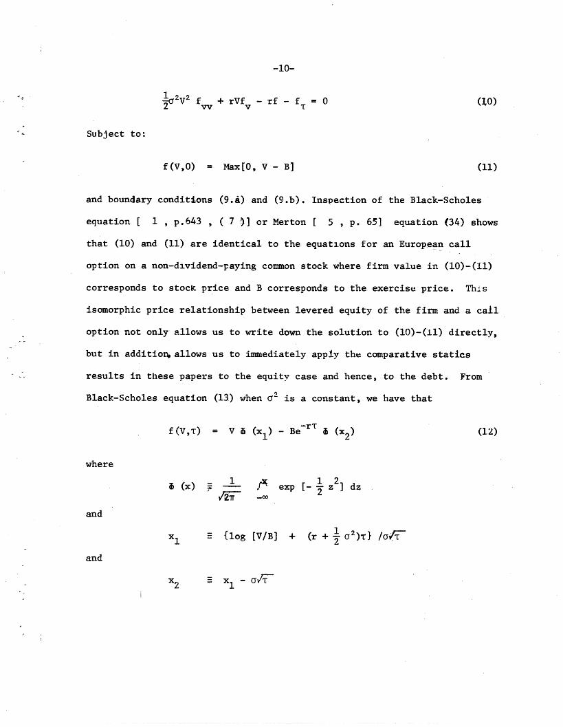
2V2 f + rVf - rf - f = (l)2 vv v T

Subject to:

f(V,O) = Max[O, V - B] (11)

and boundary conditions (9.) and (9.b). Inspection of the Black-Scholes

equation [ 1 , p.6 4 3 , ( 7 )] or Merton [ 5 , p. 65] equation (34) shows

that (10) and (11) are identical to the equations for an European call

option on a non-dividend-paying common stock where firm value in (10)-(i1)

corresponds to stock price and B corresponds to the exercise price. This

isomorphic price relationship between levered equity of the firm and a call

option not only allows us to write down the solution to (10)-(11) directly,

but in addition, allows us to immediately apply the comparative statics

results in these papers to the equity case and hence, to the debt. From

Black-Scholes equation (13.) when a 2 is a constant, we have that

f(V,T) = V (x1) - Be i (x2) (12)

where

(x) - 1 f exp [- z12 dz

and

xl - {log [V/B] + (r + o2)t} //i-

and

x 2 , X1 - /F

- 11 -

From (12) and F = V - f, we can write the value of' the debt'issue

as

F[V,T] = Be r {i [h2(da2T)] + [h (d,a2 )]} (13)

where

d - Be-r /V

hl(d,;a T' ) = -[ 2T - log(d)]/a/ri

h2 ( d,a2 1 ) - [2T + log(d)]/aciT

Because it is common in discussions of bond pricing to talk in terms of yields

father than prices, we can rewrite (13) as

R(T) - r = -1 log {[h2(d,a2T)] + [hl(d,a2t)]}'

T2d I(14)

where

exp [- R(T)Tj F(V,T)/B

and R(T) is the yield-to-maturity on the risky debt provided that the firm

does not default. It seems reasonable to call R(T) - r a risk premium in

which case equation (14) defines a risk structure of interest rates.

For a given maturity, the risk premium is a function of only

two variables: (1) the variance (or volatility) of the firm's operations, 2

and (2) the ratio of the present value (at the riskless rate) of the promised

payment to the current value of the firm, d. Because d is the debt-to-firm

value ratio where debt is valued at the riskless rate, it is a biased up-

ward estimate of the actual (market-value) debt-to-firm value ratio.

Since Merton [5] has solved the option pricing problem when the

i .................................

- 12 -

term structure is not "flat" and is stochastic, (by again using the iso-

morphic correspondence between options and levered equity) we could deduce

the risk structure with a stochastic term structure. The formulae (13) and

(14) would be the same in this case except that we would replace "exp[-rt]"

by the price of a riskless discount bond which pays one dollar at time T in

the future and "a2T" by a generalized variance term defined in [5, p. 166].

IV. A Comparative Statics Analysis of the Risk Structure

Examination of equation (13) shows that the value of the debt

can be written, showing its full functional dependence, as F[V, T, B, a", .i

Because of the isomorphic relationship between levered equity and an

European call option, we can use analytical results presented-in [5], to

show that F is a first-degree homogeneous, concave function of V and B.3

4/Further, we have that-4 /

FV = 1 - fv > 0; FB = -fB > 0 (15)

FT = -fT < 0; Fa2 = -fa2 < 0;

F = -f < 0r r

where again subscripts denote partial derivatives. The results presented

in (15) are as one would have expected for a discount bond: namely, the

value of debt is an increasing function of the current market value of the

firm and the promised payment at maturity, and a decreasing function of the

time to maturity, the business risk of the firm, and the riskless rate of

interest.

Since we are interested in the risk structure of interest rates

which is a cross-section of bond prices at a point in time, it will shed

more light on the characteristics of this structure to work with the price

- 13 -

ratio P F[V,T]/B exp[-rT] rather than the absolute price level F. P is the

price today of a risky dollar promised at time -z in the future in terms of a

dollar delivered at that date with certainty, and it is always less than or

equal to one. From equation (13), we have that

P[d,T] = P[h 2(d,T)] + [hl(d,T)] (16)

2where T c~ T. Note that, unlike F, P is completely determined by d, the

"quasi" debt-to-firm value ratio and T, which is a measure of the volatility

of the firm's value over the life of the bond, and it is a decreasing function

of both. I.e., 2

Pd - (hl)/d < 0 (17)

and

PT --'(h 1)/(2d/T) < 0 (18)

where '(x) _ exp[-x /2]//Zi is the standard normal density function.

We now define another ratio which is of critical importance in ana-

lyzing the risk structure: namely, g- y/o where fay is the instantaneous

standard deviation of the return on the bond and a is the instantaneous standard

deviation of the return on the firm. Because these two returns are instantane-

ously perfectly correlated, g is a measure of the relative riskiness of the

bond in terms of the riskiness of the firm at a given point in time.5 / From

(3b) and (13), we can deduce the formula for g to be

y = VFV/F

= [hl(d,T)]/(P[d,T]d) (19)

=g[d,T].

In Section V, the characteristics of g are examined in detail. For the pur-

poses of this section, we simply note that g is a function of d and T only, and

that from the "no-arbitrage" condition, (6), we have that

ay r

^_�_____�_III___LI�_�---(_4_·IC-�L_---�-

- 14 -

where (ay - r) is the expected excess return on the debt and (a - r) is the

expected excess return on the firm as a whole. We can rewrite (17) and (18)

in elasticity form in terms of g to be

dPd/P = -g[d,T] (21)

and

TPT/P = -g[d,T] f'(hl)/(2P(hl)) (22)

As mentioned in Section III, it is common to use yield to maturity

in excess of the riskless rate as a measure of the risk premium on debt. If

we define [R(T) - r] - H(d,T, C2), then from (14), we hav- that

1Hd= g[d,T] > 0; (23)

H22 =Ha2 = e g[d,T]['(h)/4(h)] > 0; (24)

HT = (log[P] + / g[d,T]['(hl)/<b(hl)])/T < O (25)

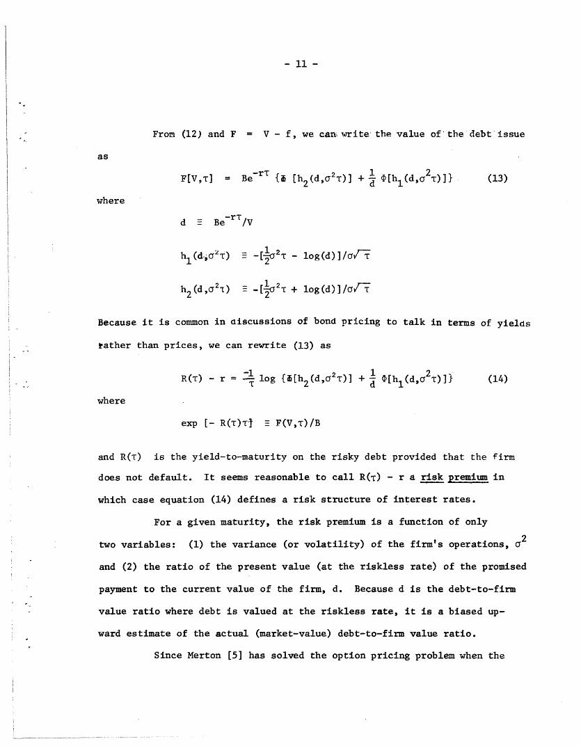
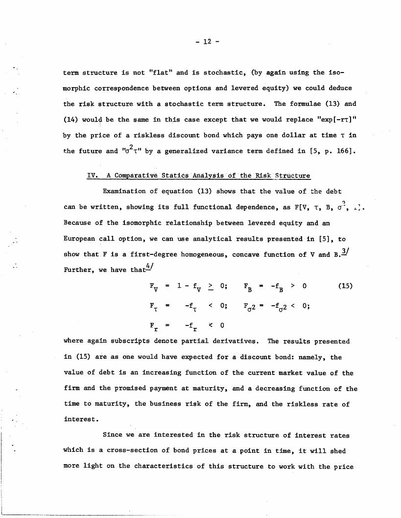
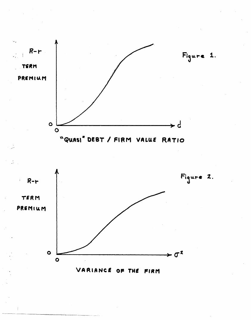
As can be seen in Figures 1 and 2, the term premium is an increasing function

of both d and a . While from (25), the change in the premium with respect to

a change in maturity can be either sign, Figure 3 shows that for

d > 1, it will be negative. To complete the analysis

of the risk structure as measured by the term premium, we show that the pre-

mium is a decreasing function of the riskless rate of interest. I.e.,

dH addr Hd ar

(26)= -g[d,T] < 0.

It still remains to be determined whether R - r is a valid measure

of the riskiness of the bond. I.e., can one assert that if R - r is larger

for one bond than for another, then the former is riskier than the latter? To

answer this question, one must first establish an appropriate definition of

"riskier." Since the risk structure like the corresponding term structure

is a "snap shot" at one point in time, it seems natural to define the riskiness

�_�_�.�_ -----· · -�s

Table I. Representative Values of the Term Premium, R - r

TIME UNTIL MATURITY

2

0.030.03

0.030.030.03

0.100.100.100.100.10

0.200.200.200.200.200) 20

d0.d0.51.0

3.0

0.2

1.0

3.0

1.01.3.0

= 2.

R-r (%)0.000.025.13

20.58.54. 4

0.010.029.74

23.0355.02.

0.123.09

14.2726.6055. 82

TIME UNTIL MATURITY =lo.

cr2

0.030.030.030.030.'03

0,100.100.100.100.10

0.200.200.200.200.20

d0.c

1.01.s3 .O

1.01.s3 .- -

0.e0.5

1.3*3.0

R-r (%)0.010.382. 444.9811-07.

0.482.124.831.12

12. 15

TIME UNTIL MAtURITY = .

2a

0.030.030.030.030.03

0.100.100. 100.100.10-

0.200.200.200.200.20

d

0.20.51.01.53.e

0.51 01.5

0.2

1.01 .b3.0

R-r(%)0.010.163.348,84

0.121.746.4711.31

0.954.239.6614.2424.30

TIME UNTIL MATURITY =.

2 .... a0.030.030.030. * 030.03

0.100.100.100.100.10

1.884.387.36

14.08

0.200.200.200.200.20

d0.e0.51.01.5

O .0.2

1.01.

0.e

1.o1.53.0

R-r(%)0.090.601- .642.57Z.S. . 4

1.072.173.394.266. 01

2.694.065. 346, 19-I J -1-

- TERM

PRE'MIuM

0

F;9&

d0

DEBT / FIRM VALUE RATIO

TERM

PREMlu

0

2.

0

VA RIANCE

i.

*'QUAISI '

Fi3 x r

OF THEe FIRM

--·---------- ---------�--·-------·---�---------------

R-r

PREMIuM

0

3,

0TIME UNTIL MATUR I TY

Igr~

- 15 -

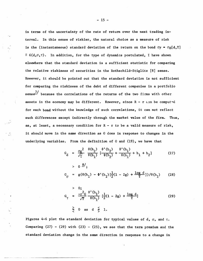
in terms of the uncertainty of the rate of return over the next trading in-

terval. In this sense of riskier, the natural choice as a measure of risk

is the (instantaneous) standard deviation of the return on the bond cry =- g[d,T]

- G(d,o,T). In addition, for the type of dynamics postulated, I have shown

elsewhere that the standard deviation is a sufficient statistic for comparing

the relative riskiness of securities in the Rothschild-Stiglitz [8] sense.

However, it should be pointed out that the standard deviation is not sufficient

for comparing the riskiness of the debt of different companies in a portfolio

7/sense- because the correlations of the returns of the two firms with other

assets in the economy may be different. However, since R - r can be computed

for each bond without the knowledge of such correlations, it can not reflect

such differences except indirectly through the market value of the firm. Thus,

as, at least, a necessary condition for R - r to be a valid measure of risk,

it should move in the same direction as G does in response to changes in the

underlying variables. From the definition of G and (19), we have that

cg2 B(h2 ) ' (h2) c'(h) (27)

Gd T(h (h2+ (hl) + h1+ h1 2(27)

> 0

G = g((h 1) - '(hl)[(1 - 2g) + --- ])/(h 1) (28)

> 0;

G = G V'(h 1) 1 2g) log dG 0 (h) [I- -g+ T (29)

0 O as d 1.

Figures 4-6 plot the standard deviation for typical values of d, a, and T.

Comparing (27) - (29) with (23) - (25), we see that the term premium and the

standard deviation change in the same direction in response to a change in

Table II. Representative Values of the Standard Deviation

of the Debt and the Ratio of the Standard Deviation

of the Debt-to-th-e- Firm, g.

TIME UNTIL MATURITY = 2.

2a

0.030.030.030.03

0.100.100.100.100.10

0.200.200.200.200.20

d0.20.51-01 *5

0.2Ob1.01.53.0

0.2

1.01.5 3.0U

g0.0000.0030.5000.9431.0U0 0..

0.0770-5000.795

.0110.168

0.7120939

TIME UNTIL MATURITY

G0.0000.0010,0870.1b3

-... 173

0,0000.0240 -1580.251.0. 03-13

0).0050.0750.2240.3180.420

=}0.

TIME UNTIL MATURITY = .

2.

0.030.030.030 .030.03

O.100.100.10

0.100.10

0.200.200.200.200.20

d

0.20.51.01.5

..... 3-.

g0.0000.0480.5QO0*833

...... 0,99 ...

O-2 0 0210.* 0.1991.0 0.3001. 5 0.689

-. 041 11 1 --- -- .s -3 -

0.2O.51.01 .3.0

0.0920.288

0.6280.815

TIME UNTIL ATUR4ITY =.

d

0. 0.51.01.53.0

0.10 0.20.10 0.*0o.10 100.10 1.50.10 .. 3.0....

0O20.5

1.53.0

g0.0030.128

0.7450 *.466

0.0920.288

0.628

0 1960.3580 *s5- 00.5840.719 3.-0 0.m22 0.278

G

0.0000.0080.0870.1440- 173

0.-0070.0630. 1580.218O.289

0.1290.2240.2810-364

2

0.03

0.03

0,03

G

0 .0 1

0.0220.0870.129

.- ..... 0~467

- 0290.0910.1. 580,199

-08-80.0880.160-0224U,2610-.321

2

0.030-030.030.03

0-.100.100.100.100.10

0.200.200.200.200.20

d

0.51.01.5-3"

0-2O *.1.01.53.0-

0.51 *.1 .5

0.200.200.200.200.20

g

0 -0560.253

-0.5000.651

. £a ..- .. 0- 57 .

0,2300.3770.50-00.5730.6-1

0.3240.4220.5000.545

G

0-.0100.0440.0870.113

. .148

0*0730.1190 -.1580.1810.219

0.1450.1890.2240,244

G

r- STANDARDDEVIA tI o

OP raD 0sT'

*1

0o 1

DEBT / FIRM VALUE RATIO

GSTANDARDItVtATI@oNoP THE

0

//9 dvl.

or0

DEVIATION

Fi3 #re

_ _ -. W I

- _ -.. _

beluts

4.

J

III

II

R3 " Ir

STANDARDO OF THE

__ ----. _.i~~____

FIRM

G

STAf1DARrDDEVIATION

OF THEDBST

0

a

i$Au.,e 6.

0

TIMlE UNTIL MATUTRITY

- 16 -

the "quasi"debt-to-firm value ratio or the business risk of the firm. How-

ever, they need not change in the same direction with a change in maturity

as a comparison of Figures 3 and 6 readily demonstrate. Hence, while compar-

ing the term premiums on bonds of the same maturity does provide a valid com-

parison of the riskiness of such bonds, one cannot conclude that a higher

term premium on bonds of different maturities implies a higher standard de-

9/viation .-

To complete the comparison between R - r and G, the standard devia-

tion is a decreasing function of the riskless rate of interest as was the

case for the term premium in (26). Namely, we have that

dG adGddr :r

(30)

= -Td Gd < 0.

V. On the Modigliani-Miller Theorem with Bankruptcy

In the derivation of the fundamental equation for pricing of cor-

porate liabilities, (7), it was assumed that the Modigliani-Miller theorem

held so that the value of the firm could be treated as exogeneous to the ana-

lysis. If, for example, due to bankruptcy costs or corporate taxes, the M-M

theorem does not obtain and the value of the firm does depend on the debt-equity

ratio, then the formal analysis of the paper is still valid. However, the

linear property of (7) would be lost, and instead, a non-linear, simultaneous

solution, F = F[V(F), ], would be required.

Fortunately, in the absence of these imperfections, the formal hedg-

ing analysis used in Section II to deduce (7), simultaneously, stands as a

proof of the M-M theorem even in the presence of bankruptcy. To see this,

imagine that there are two firms identical with respect to their investment

- 17 -

decisions, but one firm issues debt and the other does not. The investor

can "create" a security with a payoff structure identical to the risky bond

by following a portfolio strategy of mixing the equity of the unlevered firm

with holdings of riskless debt. The correct portfolio strategy is to hold

(FVV) dollars of the equity and (F - FV) dollars of riskless bonds where V

is the value of the unlevered firm, and F and FV are determined by the solution

of (7). Since the value of the "manufactured" risky debt is always F, the

debt issued by the other firm can never sell for more than F. In a similar

fashion, one could create levered equity by a portfolio strategy of holding

(fvV) dollars of the unlevered equity and (f - fvV) dollars of borrowing on

margin which would have a payoff structure identical to the equity issued

by the levering firm. Hence, the value of the levered firm's equity can never

sell for more than f. But, by construction, f + F = V, the value of the un-

levered firm. Therefore, the value of the levered firm can be no larger than

the unlevered firm, and it cannot be less.

Note, unlike in the analysis by Stiglitz [11], we did not require

a specialized theory of capital market equilibrium (e.g., the Arrow-Debreu

model or the capital asset pricing model) to prove the theorem when bank-

ruptcy is possible.

In the previous section, a cross-section of bonds across firms at

a point in time were analyzed to describe a risk structure of interest rates.

We now examine a debt issue for a single firm. In this context, we are in-

terested in measuring the risk of the debt relative to the risk of the firm.

As discussed in Section IV, the correct measure of this relative riskiness

is /a = g[d,T] defined in (19). From (16) and (19), we have that

1 + d (h 2 )g = 1 + (31)g D(h 1 )

- 18 -

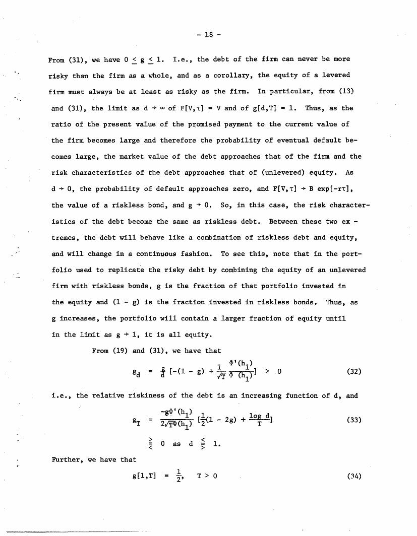
From (31), we have 0 < g < 1. I.e., the debt of the firm can never be more

risky than the firm as a whole, and as a corollary, the equity of a levered

firm must always be at least as risky as the firm. In particular, from (13)

and (31), the limit as d + X of FV,T] = V and of g[d,T] = 1. Thus, as the

ratio of the present value of the promised payment to the current value of

the firm becomes large and therefore the probability of eventual default be-

comes large, the market value of the debt approaches that of the firm and the

risk characteristics of the debt approaches that of (unlevered) equity. As

d + 0, the probability of default approaches zero, and F[V,T] -+ B exp[-rT],

the value of a riskless bond, and g + 0. So, in this case, the risk character-

istics of the debt become the same as riskless debt. Between these two ex -

tremes, the debt will behave like a combination of riskless debt and equity,

and will change in a continuous fashion. To see this, note that in the port-

folio used to replicate the risky debt by combining the equity of an unlevered

firm with riskless bonds, g is the fraction of that portfolio invested in

the equity and (1 - g) is the fraction invested in riskless bonds. Thus, as

g increases, the portfolio will contain a larger fraction of equity until

in the limit as g + 1, it is all equity.

From (19) and (31), we have that

g'(hl)g = d [-(1 - g) + d (h > 0 (32)

i.e., the relative riskiness of the debt is an increasing function of d, and

_______1 1 log dgT = [-(1 - 2g) + log d](33)

0 o as d > 1.

Further, we have that

gl,T] = 1, T > 0 (34)

�_1__1�_ �I_�___�_

- -L- ,

1- RTIO oFSTANODARD

- DEVI ATIOmSDEST / FIRM

0

"quASI DEBT / FIRM VARLE RATIO

RATIO OFSTARIDAR bI VIARMb 6Il1T / FIRI

t

F's-,,. 8.

T

I VARIANCE X TilE IANTIL MATIRITY 'at

F,-34Al-0 7.

wI

i· · bI.

i .!_.. ... ._.. .. ..

tr

A

III

I

4f

- 19 -

andlimit g[d,T] = , 0 < d < (35)T+~

Thus, independent of the business risk of the firm or the length of time

until maturity, the standard deviation of the return on the debt equals half

the standard deviation of the return on the whole firm. From (35), as the

business risk of the firm or the time to maturity get large, y + /2, for

all d.

Contrary to what many might believe, the relative riskiness of the

debt can decline as either the business risk of the firm or the time until

maturity increases. Inspection of (33) shows that this is the case if d > 1

(i.e., the present value of the promised payment is less than the current

value of the firm). To see why this result is not unreasonable, consider

the following: for small T (i.e., 2 or T small), the chances that the debt

will become equity through default are large, and this will be reflected

in the risk characteristics of the debt through a large g. By increasing T

(through an increase in or T), the chances are better that the firm value

will increase enough to meet the promised payment. It is also true that the

chances that the firm value will be lower are increased. However, remember

that g is a measure of how much the risky debt behaves like equity versus

debt. Since for g large, the debt is already more aptly described by equity

1than riskless debt. (E.G., for d > 1, g > and the "replicating" portfolio

will contain more than half equity.) Thus, the increased probability of

meeting the promised payment dominates, and g declines. For d < 1, g will

be less than a half, and the argument goes just the opposite way. In the

'"watershed" case when d = 1, g equals a half; the "replicating" portfolio

is exactly half equity and half riskless debt, and the two effects cancel

- 20 -

leaving g unchanged.

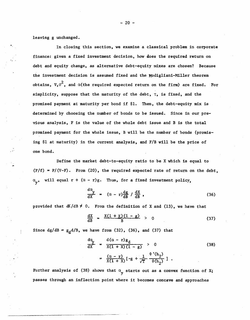
In closing this section, we examine a classical problem in corporate

finance: given a fixed investment decision, how does the required return on

debt and equity change, as alternative debt-equity mixes are chosen? Because

the investment decision is assumed fixed and the Modigliani-Miller theorem

obtains, V,a2 , and a(the required expected return on the firm) are fixed. For

simplicity, suppose that the maturity of the debt, T, is fixed, and the

promised payment at maturity per bond if $1. Then, the debt-equity mix is

determined by choosing the number of bonds to be issued. Since in our pre-

vious analysis, F is the value of the whole debt issue and B is the total

promised payment for the whole issue, B will be the number of bonds (promis-

ing $1 at maturity) in the current analysis, and F/B will be the price of

one bond.

Define the market debt-to-equity ratio to be X which is equal to

(F/f) = F/(V-F). From (20), the required expected rate of return on the debt,

al, will equal r + (a - r)g. Thus, for a fixed investment policy,

da dy = (a - r) dB (36)dX dB dB,

provided that dK/dB 0. From the definition of X and (13), we have that

dX X(1+ X)(l - g) > 0 (37)dB - '- B

Since dg/dB = gdd/B, we have from (32), (36), and (37) that

da d(a - r)g d__L > (38)dX X(1 + X)(1 - g (38)

(oa - r) [g+ 1 ' (h2X( + X) [-g (h2)

Further analysis of (38) shows that a starts out as a convex function of X;y

passes through an inflection point where it becomes concave and approaches

_I�XI_ _I_

X0

MARKE T DSBT /

9.EX PEC TED

RF T R X

o(

I,

EFgurTY RTIO

- 21 -

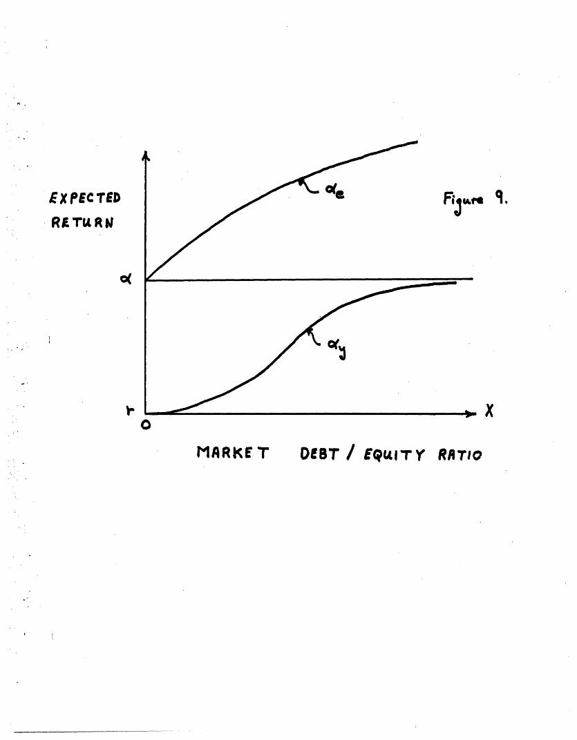
a asymptotically as X tends to infinity.

To determine the path of the required return on equity, e , as X

moves between zero and infinity, we use the well known identity that the equity

return is a weighted average of the return on debt and the return on the firm.

I.e.,

= a + X( - ay) (39)e y

= a + (1 - g) X(a - r).

ae has a slope of (a - r) at X = 0 and is a concave function bounded frome

above by the line a + (a - r)X. Figure 9 displays both a and ae . Whiley e

Figure 9 was not produced from computer simulation, it should be emphasized

that because both (ay - r)/( - r) and (e - r)/(a - r) do not depend on a,

such curves can be computed up to the scale factor (a - r) without knowledge

of a.

VI. On the Pricing of Risky Cupon Bonds

In the usual analysis of (default-free) bonds in term structure

studies, the derivation of a pricing relationship for pure discount bonds

for every maturity would be sufficient because the value of a default-free

coupon bond can be written as the sum of discount bonds' values weighted

by the size of the coupon payment at each maturity. Unfortunately, no such

simple formula exists for risky coupon bonds. The reason for this is that

if the firm defaults on a coupon payment, then all subsequent coupon payments

(and payments of principal) are also defaulted on. Thus, the default on one

of the "mini" bonds associated with a given maturity is not independent

of the event of default on the "mini" bond associated with a later maturity.

However, the apparatus developed in the previous sections is sufficient to

solve the coupon problem.

- 22 -

Assume the same simple capital structure and indenture condi-

tions as in Section III except modify the indenture condition to require

(continuous) payments at a coupon rate per unit time, C. From indenture

restriction (3), we have that in equation (7), = C = C and hence, thec

coupon bond value will satisfy the partial differential equation

22 + = 2 F+ (rN,- ) F -r - + =0 (40)

subject to the same boundary conditions (9). The corresponding equation

for equity, f, will be

u o = f + (rV - C) f - rf - f (41)VV v T

subject to boundary conditions (9a), (9b), and (11). Again, equation (41)

has an isomorphic correspondence with an option pricing problem previously

studied. Equation (41) is identical to equation (44) in Merton [5, p.170]

which is the equation for the European option value on a stock which pays

dividends at a constant rate per unit time of C. hile a closed-form

solution to (41) or finite T has not yet be found, one has been found for

the limiting case of a perpetuity (T = o), and is presented in Merton [5, p. 172,

equation (46)]. Using the identity F = V - f, we can write the solution for

the perpetual risky coupon bond as 2r2

F(Vl) Cl- 2r 2r 2r -2Ci(2+-M 2 + (o- +7- ))(2+ F -)

where r ( ) is the gamma function and M ( ) is the confluent hypergeomel

function. While perpetual, non-callable bonds are non-existent in the

United States, there are preferred stocks with no maturity date

(42) would be the correct pricing function for them.

Moreover, even for those cases where closed-form solutions

cannot be found, powerful numerical integration techniques have been

(42)

tric

and

- 23 -

developed for solving equations like (7) or (41). Hence, computation and

empirical testing of these pricing theories is entirely feasible.

Note that in deducing (40), it

was assumed that coupon payments were made unitormly ana continuously. In

fact, coupon payments are usually only made semi-annually or annually in

discrete lumps. However, it is a simple matter to take this into account

by replacing "C" in (40) by " iCi (T-Ti)" where ( ) is the dirac delta

function and T. is the length of time until maturity when the Ith coupon1

payment of C. dollars is made.

As a final illustration, we consider the case ot callable bonds.

Again, assume the same capital structure but modify the

indenture to state that "the firm can redeem the bonds at its option for a

stated price of K(T) dollars" where K may depend on the length of time until

maturity. Formally, equation (40) and boundary conditions (9.a) and (9.c)

are still valid. However, instead of the boundary condition (9.b) we have

that for each T, there will be some value for the firm, call it V(T), such

that for all V(T) > V(T), it would be advantageous tor the firm to redeem

the bonds. Hence, the new boundary condition will be

F[V(T), T] = K(T) (43)

Equation (40), (9.a), (9.c), and (43) provide a well-posed problem to solve

for F provided that the V(T) function were known. But, of course, it is not.

Fortunately, economic theory is rich enough to provide us with an answer.

First, imagine that we solved the problem as if we knew V(T) to get

F[V,T; V(T)] as a function of V(T). Second, recognize that it is at manage-

ment's option to redeem the bonds and that management operates in the best

interests of the equity holders. Hence, as bondholder, one must presume that

�_I� _ � �_�__11�___�1 �1_ II��__��___

- 24 -

management will select the V(T) function so as to maximize the value of equity,

f. But, from the identity F = V - f, this implies that the V(T) function chosen

will be the one which minimizes F[V,T; V(T)]. Therefore, the additional

condition is that

F[V,T] = min F[V,T; V(T)] (44){V(T) }

To put this in appropriate boundary condition form for solution, we again

rely on the isomorphic correspondence with options and refer the reader to

the discussion in Merton [5] where it is shown that condition (44) is

equivalent to the condition

F[V(T),T] = 0

Hence, appending (45) to (40), (9.a), (9.c) and (43), we solve tne problem

for the F[V,T] and V(T) functions simultaneously.

V. Conclusion

We have developed a method for pricing corporate liabilities

which is grounded in solid economic analysis; required inputs which are on

the whole observable; can be used to price almost any type of financial in-

strument. The method was applied to risky discount bonds to deduce a risk

structure of interest rates. The Modigliani-Miller theorem was shown to

obtain in the presence of bankruptcy provided that there are no differential

tax benefits to corporations or transactions costs. The analysis was

extended to include callable, coupon bonds.

FOOTNOTES

Associate Professor of Finance, Massachusetts Institute of Technology.I thank J. Ingersoll for doing the computer simulations and forgeneral scientific assistance. Aid from the National Science Founda-tion is gratefully acknowledged.

1. Of course, this assumption does not rule out serial dependence inthe earnings of the firm. See Samuelson [10] for a discussion.

2. For a rigorous discussion of Ito's Lemma, see McKean [4]. For refer-ences to its application in portfolio theory, see Merton [5].

3. See Merton [5, Theorems 4, 9, 10] where it is shown that f is a first-degree homogeneous, convex function of V and B.

4. See Merton [5, Theorems 5, 14, 15].

5. Note, for example, that in the context of the Sharpe-Lintner-MossinCapital Asset Pricing Model, g is equal to the ratio of the 'beta"of the bond to the "beta" of the firm.

6. See Merton [5, Appendix 2].

7. For example, in the context of the Capital Asset Pricing Model, thecorrelations of the two firms with the market portfolio could be suf-ficiently different so as to make the beta of the bond with thelarger standard deviation smaller than the beta on the bond with thesmaller standard deviation.

8. It is well known that '(x) + x(x) > 0 for - < x a< .

9. While inspection of (25) shows that HT < 0 for d > 1 which agreeswith the sign of GT for d > 1, HT can be either signed for d < 1which does not agree with the positive sign on G .

Bibliography

1. Black, F. and Scholes, M., "The Pricing of Options and Corporate Lia-bilities," Journal of Political Economy (May-June 1973).

2. , "The Valuation of Option Contracts and a Testof Market Efficiency", Journal of Finance (May 1972).

3. Fama, E.F., "Efficient Capital Markets: A Review of Theory and EmpiricalWork", Journal of Finance (May 1970).

4. McKean, H.P., Jr., Stochastic Integrals, New York, Academic Press, 1969.

5. Merton, R.C., "A Rational Theory of Option Pricing", Bell Journal of

Economics and Management Science (Spring 1973).

6. , "Dynamic General Equilibrium Model of the Asset Market andand Its Application to the Pricing of the Capital Structure of the Firm",SSM W,P. #497-70, M.I.T. (December 1970).

7. Miller, M. and Modigliani, F., "The Cost of Capital, Corporation Finance,and the Theory of Investment", American Economic Review (June 1958).

8. Rothschild, M. and Stiglitz, J. E., "Increasing Risk: I. ADefinition," Journal of Economic Theory, Vol. 2, No. 3(September 1970).

9. Samuelson, P. A., "Proof that Properly Anticipated Prices FluctuateRandomly," Industrial Management Review (Spring 1965).

10. , "Proof that Properly Discounted Present Values ofAssets Vibrate Randomly," Bell Journal of Economics and ManagementScience, Vol. 4, No. 2 (Autumn 1973).

11. Stiglitz, J. E., "A Re-Examination of the Modigliani-Miller Theorem,"American Economic Review, Vol. 59, No. 5 (December 1969).