on the rationality of medium-term tax revenue forecasts ... · tax revenue forecasts: evidence from...

On the Rationality of Medium-Term Tax Revenue Forecasts: Evidence from Germany

Christian Breuer

Ifo Working Paper No. 176

March 2014

An electronic version of the paper may be downloaded from the Ifo website www.cesifo-group.de.

Ifo Institute – Leibniz Institute for Economic Research at the University of Munich

Ifo Working Paper No. 176

On the Rationality of Medium-Term Tax Revenue Forecasts: Evidence from Germany*

Abstract

In the present paper I examine tax revenue projections in Germany over the period 1968

to 2012 with a focus on forecasting rationality. I show that tax revenue forecasts for the

medium-term are upward biased. Overoptimistic revenue projections are particularly

pronounced after the German reunification and reflect upward-biased GDP projections

in this period. The predicted tax-GDP-ratio appears to be upward biased, as well. The

forecasts are likely to overestimate tax revenues if the predicted tax-GDP-ratio exceeds

its structural level of approximately 22 ½ percentage points. The results also indicate

that forecast errors of short-term projections for the current year exhibit serial correlation.

It is conceivable that the specific institutional setting can explain this non-rational

behaviour to some extent.

JEL Code: E62, H20, H68.

Keywords: Tax revenue forecasting, forecast rationality, budgetary Planning.

Christian Breuer Ifo Institute – Leibniz Institute for

Economic Research at the University of Munich

Poschingerstr. 5 81679 Munich, Germany

Phone: +49(0)89/9224-1265 [email protected]

* The author is member of the Working Group on Tax Revenue Forecasting (Arbeitskreis “Steuerschätzungen”), an advisory group at the German Federal Ministry of Finance (BMF).

mailto:[email protected]

2

1. Introduction

Public budgeting receives increasing attention in the course of the fiscal crisis in the Eurozone

and other OECD countries. The Treaty on Stability, Coordination and Governance (TSCG) in

the Economic and Monetary Union (EMU) gives rise to a stronger focus on budgetary

planning and monitoring at the European level. For European countries, a newly adopted

fiscal rule postulates a tight limit of a structural budget deficit of 0.5 % of the gross domestic

product (Art. 5 TSCG).

Accurate revenue forecasts are necessary to meet the budgetary targets. Chatagny and Soguel

(2012) show that tax revenue forecast errors influence the budget balance, probably because

overestimated revenue projections may be a substitute for explicit deficits in legislative

budgets (Bischoff and Gohout, 2010). The analysis and improvement of fiscal planning and

revenue forecasting practices is, thus, of interest for the scientific community as well as

policymakers.

In Europe, Germany is seen as an example for successful public budgeting. Tax revenue

forecasting has a long tradition in Germany. Since 1955 the Working Group on Tax Revenue

Forecasting (AKS)1, an advisory board at the federal ministry of finance, provides official tax

revenue forecasts for the purpose of public budgeting in Germany.2

It is, however, controversial whether tax revenue projections in Germany are unbiased and

efficient. Only a few studies analyse the rationality of tax revenue forecasts. A large part of

the literature focuses on revenue forecasting at the federal level. According to Heinemann

(2006), the forecasts of the tax-GDP-ratio in the medium-term financial plans at the federal

level do not pass standard tests of (weak) rationality. In this line the German Federal Court of

Auditors criticised the forecasting quality of the AKS. The forecasts appear to be over-

1 Arbeitskreis “Steuerschätzungen” (AKS).

2 See Fox (2005) on the institutional background and the history of the AKS.

3

optimistic and the Court proposed to examine the methodology of the AKS

(Bundesrechnungshof, 2006). Recent studies, however, did not confirm that tax revenue

forecasts in Germany are over-optimistic. They state that tax revenue forecasts at the federal

level are unbiased in the short-run (Becker and Büttner, 2007, Lehmann, 2010, Büttner and

Kauder, 2011). In a comprehensive study, Gebhardt (2001) examines the forecasting quality

of tax revenue projections by the AKS. He stresses that the AKS provides conditional

forecasts and that the forecast errors of the AKS may reflect overoptimistic GDP projections

or inaccurate revenue estimations of tax policy changes.

Recent studies analyse the influence of political factors (Bischoff and Gohout, 2010, Büttner

and Kauder, 2011,). Election-motivated politicians may try to manipulate revenue forecasts to

increase the probability of re-election. In Germany, however, politicians hardly influence tax-

revenue forecasts because the AKS is strongly independent (Büttner and Kauder, 2010). The

federal government can, however, influence tax revenue forecasts by biasing the

macroeconomic forecast of the government (which is conditional for tax revenue forecasters),

or by tax policy changes (Gebhardt, 2001).

This study contributes to the discussion on the rationality of German tax revenue projections

by examining a new dataset on medium-term tax revenue forecasts over the period 1968 to

2012. Contrary to previous research I show that tax revenue forecasts for the medium-term are

upward biased. Overoptimistic revenue projections are particularly pronounced after the

German reunification and reflect upward-biased GDP projections in this period. The forecasts

are likely to overestimate tax revenues if the predicted tax-GDP-ratio deviates from its

structural level of approximately 22 ½ percentage points. The results also indicate that

forecast errors of short-term projections for the current year exhibit serial correlation.

4

2. Institutional Background

Since 1955, the AKS conducts tax revenue forecasts for the purpose of budgetary planning in

Germany. The AKS meets regularly twice a year. At the end of every year, usually in

November, the AKS provides official revenue forecasts for the next year’s budget. It includes

an update for the expected value of revenues in the current year t and a forecast for the next

year (budget year) t+1 (short–run horizon). The tax projections are the predominant

component of the revenue-side budget and determine the maximum level of expenditures in

the legislative budget under a given fiscal rule.3

Since 1968 the AKS produces revenue forecasts for the medium-term budgetary plan

(regularly in May). The German federal government introduced medium-term fiscal planning

after the first post-war recession in 1967. In contrast to the federal budget, the medium-term

financial plan is not adopted by the parliament and not legally binding. It represents, however,

planning intentions of the government.4

The AKS consists of representatives of the federal government, the central bank

(Bundesbank), the German Council of Economic Experts (Sachverständigenrat), economic

research institutes5, the German States (Laender), the German cities council, and the federal

statistical office. Before the AKS meetings, the federal government, the German central bank,

the Council of Economic Experts and the economic research institutes individually provide

unpublished tax revenue projections. All individual projections are, however, based on unique

3 The newly adopted fiscal rule in Germany restricts the structural deficit of the federal budget to 0.35% of GDP.

4 See Heinemann (2006), Lübke (2008), and Breuer et al. (2011) on medium-term fiscal planning at the federal

level in Germany. 5 The Institute for the World Economy at the University of Kiel (IfW), the Halle Institute for Economic Research

(IWH), the Rheinisch-Westfälisches Insitut für Wirtschaftsforschung (RWI) Essen, the German Institute for

Economic Research (DIW) Berlin and the Ifo Institute – Leibniz Institute for Economic Research at the

University of Munich (ifo) represent the German research institutes at the AKS.

5

assumptions about the macroeconomic outlook and conditional to the macroeconomic

forecast of the federal government.6

The AKS enjoys a relatively high degree of independence, compared to international

standards (Büttner and Kauder, 2011) because a large number of non-governmental

institutions participate at the AKS meetings. The government would be able to influence the

tax revenue projections of the AKS only by a strategic setting of the macroeconomic forecast

and by changes in tax policy, which are both conditional for the AKS forecast. Tax

projections are based on assumptions about the impact of changes in tax policy and, thus, tax

revenue forecast errors may result from erroneous assumptions about tax policy (Auerbach,

1999 and Gebhardt, 2001). The AKS assumes no future changes in tax policy, if the change

didn’t pass the legislative process at the time of the forecast. The AKS incorporates revenue

effects of changes in tax policy only when the appropriate bill passed the parliamentary

process. Since policy-makers often change the tax code, these changes might significantly

influence revenue forecast errors, particularly in the medium-term.

The AKS produces a joint tax revenue forecast at the general government level. Later, the

AKS distributes the estimated sum of total tax revenues at the general government level to the

territorial entities, the federal level, the state level and municipalities (regionalization).

Different from previous analyses of fiscal forecasts at the federal – or state level (Heinemann,

2006, Bischoff and Gohout, 2010, Büttner and Kauder, 2011), in this paper I analyse tax

revenue forecasts of the AKS at the general government level. I do not analyse forecast errors

at the federal or state level to abstract from changes in the regional distribution of tax

revenues.

6 The VAT revenue forecast is based on the forecast of the level of private consumption. The wage tax is linked

to the expected growth rate of the national wage bill, and expected employment. See Körner (1983), Flascha

(1985) and Gebhardt (2001) on the revenue dynamics of selected taxes and on the relationship between selected

taxes and their tax bases.

6

3. Data and Descriptive Statistics

After the meeting of the AKS, the federal ministry of finance publishes the results of the

official tax revenue forecast and releases a press statement (BMF 1968 – 2012a; BMF 1968 –

2012b). In the present study, I use data on tax revenue forecasts and respective forecasts of

the nominal GDP by the federal government (GNP before 1994) for the current year (t) to the

fourth year to the future (t+4) based on the regular AKS reports during the years 1968 to

2012. To construct forecast errors for tax revenue projections at time t for the year t+h, I use

the first official realization, which is available in the AKS reports of the year t+h+1, where t

denotes the date of the forecast and h indicates the forecast horizon.

The GDP forecast error

is the difference between realization t t h and forecast

of

the GDP growth rate for year t+h at time t:

t t h

(1)

The tax revenue forecast error is the difference between realization and forecast of the growth

rate of tax revenues r for the year t+h at time t:

t t h

(2)

Finally, the forecast error of forecast for the tax-GDP-ratio q is

t t h

rt t h

t t h

rt t h

t t h

(3)

7

Figure 1 shows the forecast errors of tax revenue forecasts, the appropriate GDP projections

and the tax-GDP-ratio. A positive value indicates an underestimation (of tax revenues, GDP

or the tax ratio), and a negative coefficient denotes an overestimation. I classify forecast

errors of the same forecast made in year t with the number 0 to 4, indicating the forecast

horizon h. In this study, the forecast error of the year 1968 with the forecast horizon 4

describes the forecast error of a revenue projection made in the year 1968 and projecting

revenues for the year 1972.

The German reunification causes a structural break in the time series. German federal taxes do

not distinguish between new and old German Laender. Because of this, forecast errors of

forecasts made in a year before reunification, predicting revenues for a year after the

reunification contain a bias. Therefore, I exclude forecasts conducted before 1991 and

predicting periods after 1991 to control for the effect of reunification. I distinguish between

two periods: (1) the pre-reunification period 1968 – 1990 and (2) the post-reunification

period, starting in 1991.

Table 2.1 shows standard measures of forecasting quality, the mean error (ME), mean

absolute error (MAE), root mean squared error (RMSE) and Theil’s (1966) inequality

coefficient (U) for the forecast errors of tax revenues, GDP and the tax-GDP-ratio. The mean

error shows a negative sign for multi-year forecasts, indicating a propensity to overestimate

tax revenues. The prediction quality decreases with the forecast horizon h, since the MAE and

the RMSE increase with h. Theil’s inequality coefficient compares the observed mean square

error to the mean squared error of a benchmark forecast. I define the benchmark projection as

the last observed value in the year prior to conducting the forecast. If the coefficient exceeds

one, the benchmark forecast would improve the prediction quality of the forecast at the

respective horizon. A comparison between the benchmark forecast and the forecast by the

AKS shows that the AKS forecasts of tax revenues and of GDP perform better than a

benchmark forecast. A naïve projection of the tax-GDP-ratio would better match the future

8

tax ratio than the AKS forecast in the medium-term. Given a conditional forecast for GDP, it

is conceivable that a naïve extrapolation of tax revenues, keeping the tax-GDP-ratio constant,

improves the forecasting quality of the AKS.

4. Empirical Analysis

A) Unbiasedness

Rational forecasts presuppose unbiasedness and efficiency. An unbiased forecast implies that

the mean forecast error is not significantly different from zero. To test for unbiasedness,

Holden and Peel (1990) suggest estimating the condition of in the following equation:

, (4)

where is the forecast error of the h-step ahead forecast of tax revenues

at time t

and denotes the realized tax revenue at time t+h. I apply equation (4) for the analysis of

tax revenue forecasts, GDP forecasts and forecasts of the tax-GDP-ratio. The forecasts are

unbiased if the null-hypothesis of unbiasedness ( ) cannot be rejected.

B) Weak rationality

The literature on forecasting accuracy applies models in the tradition of Mincer and Zarnowitz

(1969), to test for (weak) rationality (Feenberg et al. 1989):

(5)

9

here rt t hf

describes the h-step ahead revenue forecast at time t, and ut is an error term which

coincides with the forecast error when the forecast is unbiased (Mocan and Azad, 1995). I

rearrange (2) to obtain the forecast error on the left-hand side:

(6)

Weak rationality requires that . While a positive (or negative) coefficient

suggests a tendency towards under- (or over-) estimation, the coefficient ( - ) indicates a

relationship between the forecast value and the forecast error. The forecasts are (weakly)

rational, if the individual null hypothesis cannot be rejected.

C) Strong rationality

Strong rationality implies that the forecast is unbiased and efficient. An efficient forecast

contains all relevant information that is available at the time of the forecast (Nordhaus, 1987).

I test for efficiency by using equation (7), where represents n variables assumed to be part

of the information set of the forecaster at time t:

∑

(7)

If we cannot reject the null-hypothesis ( , the forecasts

are efficient and, thus,

(strongly) rational. include the previous year’s forecast error for the current-year forecast

(forecast revision for year t-1) to test for serial correlation of forecast errors. Additionally, I

include the projected tax-GDP-ratio. Moreover, it is conceivable that forecasts appear to be

particularly optimistic in a certain macroeconomic environment, i. e. when budget deficits are

10

large, or in times of economic crisis. Particularly in times of large budget deficits,

governments might tend to produce over-optimistic forecasts. To control for these factors, I

additionally include the (previous year’s) general government deficit as ell as the (lagged)

GDP growth rate, and assume that both variables are part of the information set of the

forecasters at the time when the forecast is made.

5. Results

A) Unbiasedness

Table 2 shows the results of equation (4), the coefficients ( ) and the respective standard

errors. The coefficients for h > 0 are negative, indicating that the AKS overestimated tax

revenues for multi-year forecasts during the period 1968 – 2011. Forecasts with multi-year

forecast horizons are prone to autocorrelation (McNees, 1978). All numbers in parentheses

report autocorrelation-consistent (Newey-West) standard errors.7

Panel A) shows that tax revenue forecasts for the current and the subsequent year are

unbiased, however, the mean error for the horizon h = 4 is 7.2 % and significant at the 10 %

level (row no. 5). The results are not very pronounced before the reunification, but statistically

significant for medium-term forecasts after 1991. After the reunification, the forecasts

overestimated tax revenues on average by 10.9 % at the end of the forecast horizon (h = 4).

The results are, however, sensitive to sample variations.

7 The Durbin-Watson statistics indicate the presence of positive autocorrelation, particularly for medium-term

forecasts.

11

Figure 2 shows the results of recursive estimations of equation (4) for different forecast

horizons (h … 4). For short-run tax revenue forecasts, the coefficient does not turn

out to be statistically significant at conventional levels for any sample variation. Forecasts for

the medium-term start (e. g. h = 4) with a positive coefficient , indicating that the AKS

underestimated tax revenues at the beginning of the sample in the late 1960s and early 1970s.

The coefficient decreases in the 70s and changes the sign in the 80s, reflecting a tendency

towards overestimation in this period. The coefficient increases again after 2003, indicating

that the forecasts are less overoptimistic after 2003. The right-hand side of figure 2 displays

recursive estimations of the post-reunification sample, starting in 1991. The coefficient

appears to be negative at all horizons. The forecasts are particularly prone to over-optimism in

the post-reunification episode. The results are significant already for the short-run (h = 1), but

particularly striking for medium-term forecasts. The tendency towards over-optimism

decreases after 2003, but the overoptimistic bias for multi-year forecasts (horizon 2, 3 and 4)

is statistically significant for the entire post-reunification sample.

The GDP projection of the federal government has been overoptimistic during the period

1968 and 2011 as well (row no. 6 to 10 of table 2). The overoptimistic bias of the GDP

forecast is particularly pronounced and statistically significant at conventional levels only

after reunification, indicating that the forecast uncertainty of GDP projections after German

reunification increased and the positive expectations in the aftermath of the German

reunification have not been realized. The bias is significant after reunification, already for

forecasts with the horizon h=1 (short-run). It seems that the overoptimistic GDP projections

after reunification influenced the overoptimistic tax revenue forecasts, so that the forecast of

the tax-GDP-ratio does not exhibit a significant bias in this period (row no. 11 to 15).

Panel C) of table 2 shows the results of equation (4) for the tax-GDP-ratio. The results show

that we can reject the hypothesis of unbiasedness for forecasts of the tax-GDP-ratio with the

horizon 3 and 4 (row no. 14 and 15). The projected tax-GDP-ratio, thus, exhibits an

12

overoptimistic bias. The bias increases with the forecast horizon. At the end of the forecast

horizon (h=4) the AKS overestimated the tax-GDP-ratio by 0.64 percentage points. This

result is statistically significant at the 5 % level.

B) Weak rationality

Table 3 shows the results of the tests for weak rationality. Row no. 1 to 5 show the results for

tax revenue forecasts, and row no. 6 to 10 depict the results for GDP projections of the federal

government. The results show that we cannot reject the hypothesis of (weak) rationality for

both, tax revenues and GDP projections, at all horizons (h …4). The forecasts of the

tax-GDP-ratio, however, do not pass the tests of weak rationality. The respective F-statistics

reject the hypothesis that = 1 - 0 at conventional levels (p-value < 10 %). The results

are stronger pronounced for medium-term forecasts, but even short-run forecasts of the tax-

GDP-ratio are not (weakly) rational (row no. 11). Equation (5) implies that if the tax ratio

forecast denoted by the coefficient -

-

is exceeded, the forecast is likely to overestimate the

tax-GDP-ratio. According to the results in table 3, this coefficient turns out to be close to the

historical trend of the tax-GDP-ratio of 22 ½ percentage points.

C) Strong Rationality

Table 4 shows the results of equation (7), where includes variables that are part of the

information set when the forecasts are made. I include the previous year’s forecast error for

the current-year forecast (forecast for year t-1 made in t-1) to test for serial correlation of

forecast errors. It is conceivable that forecasts appear to be particularly optimistic in a certain

macroeconomic environment, e. g. when deficits are large, or GDP growth is low. To control

13

for these factors I additionally include the (previous year’s) general government deficit the

(previous year’s) GDP gro th rate as ell as the predicted tax-GDP-ratio, which are part of

the information set of the forecasters at time t.

The AKS forecast of tax revenues do not pass this test for (strong) rationality. The results in

table 4 suggest that forecast errors of projections for the very short-run (current year) exhibit

positive serial correlation (column 1). It is, thus, likely that the AKS forecast for the current

year is overoptimistic if the forecast of last year’s tax revenues turned out to be

overoptimistic as well. Serial correlation in revenue forecast revisions seems to be a prevalent

issue. Auerbach (1999) pointed to the appearance of serial correlation of tax revenue forecast

revisions in the United States. For multi-year forecasts, however, the results do not indicate

that previous errors determine future forecast errors. Tax revenue forecasts are, however,

likely to overestimate tax revenues if the projected tax-GDP-ratio exceeds –

. The critical tax

ratio –

, again, turns out to be close to the structural tax ratio of approximately 22 ½ percent.

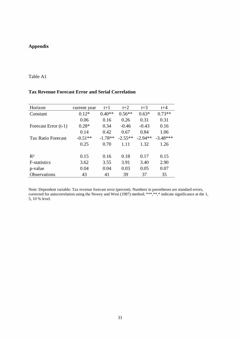
In table, I repeat the regressions of equation (7), but exclude variables that turn out to be

insignificant for most of the specifications, and test, whether the predicted tax-GDP-ratio,

influences the tax revenue forecast error. I do not include (lagged) forecast error for the

horizon t=0, because it has been significantly affecting the forecast error only in column 1 of

table 2.4.8 The predicted tax-GDP-ratio turns out to be significantly correlated with the

forecast error of tax revenues with the same horizon in most of the specifications, indicating

that the predicted tax-GDP-ratio influences the tax revenue forecast error. The p-value of the

appropriate F-statistics shows that we can reject the hypothesis of (strong) rationality at every

horizon. The results are particularly pronounced for multi-year forecasts, but statistically

significant for short-run tax revenue forecasts, as well.

8 I show the results, including the lagged forecast error for current year’s forecasts, in the appendix.

14

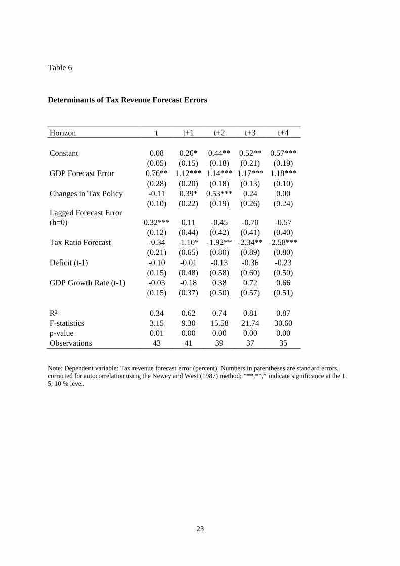
6. Determinants of Forecast Errors

The results, as presented in table 4 and 5 imply that the AKS fails to forecast tax revenues

efficiently. It is, however, conceivable that other unknown determinants influence the forecast

error (unobserved variable bias). To account for other factors and to analyse the determinants

of tax revenue forecast errors, I apply regressions of equation (7), where includes

determinants of tax revenue forecast errors, known or unknown a time t. I include the GDP

forecast error of the GDP forecast by the government with the same forecast horizon, as well

as tax policy changes to account for the influence of political and economic factors. Both

variables are not available at the time when the forecast is made, but certainly influence the

forecast error of tax revenue forecasts.9 The variables are influenced by decisions of the

federal government, so that it is worthwhile to analyse whether the test for efficiency shows

the same results after controlling for these factors. Figure 3 depicts the estimated influence of

tax policy changes on tax revenues, based on published calculations by the German federal

government.10

Table 6 shows the estimated influence of potential determinants on the tax revenue forecast

errors. It turns out that the GDP forecast error positively influences the tax revenue forecast at

every horizon. The coefficient is approximately one, what is in-line with assumptions about

the GDP elasticity of tax revenues. Moreover, changes in tax policy affect the forecast error

positively.

9 In this line Büttner and Kauder (2011) analyze the influence of GDP forecast errors, as well as changes in tax

policy, on short-term revenue forecast errors. 10

Since 1967, the German federal government estimates the impact of tax policy changes at the general

government level and publishes the estimations in the annual reports of the federal ministry of finance (BMF,

1968-2012c). For every year t, I calculate the sum of the estimated impact of changes in tax policy, and

after ards the estimated impact per (last year’s) tax revenue.

15

The estimated coefficient, however, turns out to be low, indicating that the estimated impact

of tax policy is overestimated.11

The integration of GDP errors and tax policy changes,

however, does not diminish the effect of serial correlation in current year forecast errors

(column 1). Moreover, the estimated tax ratio has a significant positive influence on the

forecast error, indicating that an above-average forecast of the tax ratio increases the

likelihood of an overoptimistic tax revenue forecast, even after controlling for GDP forecast

errors and tax policy changes. These findings suggest, that GDP forecast errors, as well as tax

policy changes (tax cuts), do not explain the forecast errors of the predicted tax-GDP-ratio.

The effects of (previous year’s) deficit and gro th ho ever does not have a significant

impact on the tax revenue forecast error.

7. Conclusion

In the present paper I analyse the forecasting performance of the official tax revenue

projections in Germany. Tax revenue forecasts and the forecasts of the tax-GDP-ratio are

overoptimistic for projections in the medium-term. The overoptimistic bias of tax revenue

forecasts, as well as GDP projections is particularly pronounced after the German

reunification, so that the overoptimistic tax revenue projections may reflect overoptimistic

GDP forecasts made by the federal government. It is conceivable that the uncertainty about

11

It is conceivable that the government overestimates the revenue effect of policy changes and probably

underestimates the potential feedback effects of tax changes on GDP. The estimation is based on assumptions

about the timing of tax policy and it is conceivable that it is not possible to account perfectly for the influence of

tax policy changes on revenue forecast errors with the measure of tax policy. For the regressions in table 6, I e. g.

assume that tax policy in year t influences tax revenue forecast errors of the same year (column 1). For forecasts

ith the horizon 1 I assume that next year’s tax policy changes influence the forecast error (of forecasts made in

year t). Fore medium-term forecasts, I assume that all tax policy changes in the forecast horizon influence the

forecast error, but excluding policy changes in a year when the forecast is made. This treatment is based on the

assumption that the tax revenue forecasts do not include policy changes for the next year, because these policy

changes didn’t pass the parliamentary process at the time hen the AKS meets (regularly in May).

16

potential GDP in the aftermath of the German reunification contributed to the overoptimistic

bias of the GDP- and tax revenue forecasts, or that a decrease in trend growth rates affected

GDP forecast errors for the medium-term in this period. It is also conceivable that the federal

government decided to overestimate GDP and to improve fiscal forecasts in the medium-term

budget outlook in order to cover the true costs of the German reunification. The propensity

towards overestimation, however, decreased after 2004. Upward-biased GDP-projections and

tax revenue forecasts may, thus, be a transitory phenomenon.

To avoid a suspicion that the federal government may influence tax revenue forecasts for a

political purpose by strategically influencing the conditional macroeconomic forecast, it

would be reasonable to rely on a more independent macroeconomic projection and by

providing more independence to the AKS (Heinemann, 2006). The independent economic

research institutes that are involved in the ‘Gemeinscha tsdiagnose’ (GD)12

prepare a

macroeconomic forecast just before the government present its macroeconomic forecast.13

It

would be worthwhile to use the joint economic forecast as the conditional benchmark

projection for fiscal planning in Germany to avoid a possible political influence.

The forecasts of the tax-GDP-ratio fail tests for efficiency. My results show that short-run

forecasts for the current year exhibit serial correlation. Additionally, if the forecasts of the

tax-GDP-ratio deviates from the structural level (of approximately 22½ %), the forecasts are

likely to over-/underestimate this ratio as well as the amount of tax revenues. According to

my results, even a naïve projection of the tax-GDP-ratio for the medium term exhibits a better

forecast quality than the AKS forecast. Keeping the tax-GDP-ratio constant would improve

the forecasting accuracy of the AKS in the medium-term.

12

A joint economic forecast of different research institutes on behalf of the federal government in Germany. 13

See Kirchgässner and Savioz (2001), Döpke and Fritsche (2008), and Döhrn and Schmidt (2011) on the joint

economic forecast in Germany.

17

The AKS forecast is a conditional forecast based on assumptions about the macroeconomic

outlook and tax policy changes.14

It is conceivable that overoptimistic GDP projections and

regular tax reductions cause non-rational revenue projections. After controlling for the

estimated impact of policy changes and GDP growth forecast errors, however, the results

remain quite unchanged. Identifying the true reasons for a non-rational behaviour of

government revenue forecasts in Germany would be a challenge for future research.

Acknowledgements

I thank Alfred Boss, Jens Boysen-Hogrefe, Thiess Büttner, Gebhard Flaig, Ulrich Fritsche,

Heinz Gebhardt, and Christian Merkl for very helpful comments, hints and suggestions.

14

See Don (2001) and Gebhardt (2001) on the problem of conditional forecasts.

18

Table 1

Summary Statistics

A) ME (%)

Tax revenue GDP tax-GDP-ratio

current year 0.27 0.03 0.01

year t+1 -0.39 -0.53 -0.07

year t+2 -2.23 -1.55 -0.28

year t+3 -4.68 -3.14 -0.49

year t+4 -7.20 -4.96 -0.64

B) MAE (%)



year t+1 4.82 2.83 0.70

year t+2 7.86 5.20 1.00

year t+3 10.59 7.40 1.01

year t+4 14.00 10.16 1.04

C) RMSE



year t+1 6.07 3.59 0.85

year t+2 9.38 6.35 1.19

year t+3 12.49 9.10 1.28

year t+4 16.60 12.37 1.32

D) Theil's U



year t+1 0.58 0.51 0.89

year t+2 0.57 0.60 1.09

year t+3 0.53 0.58 1.13

year t+4 0.51 0.56 1.09

Note: The table shows the mean error (ME), mean absolute error (MAE), root mean squard error (RMSE), as

ell as the Theil’s inequality coefficient (Theil’s U) for tax revenue forecasts GDP forecasts as ell as

predicted tax-GDP-ratios, with the horizon 0 to 4.

19

Table 2

Tests of Unbiasedness

Row

no. h

Full

Sample D-W

Pre-

Reunification

Post-

Reunification

A) Tax revenue

1 0 0.27 (0.33) 1.49 0.19 (0.31) 0.36 (0.61)

2 1 -0.39 (1.05) 1.19 0.32 (1.34) -1.17 (1.66)

3 2 -2.23 (1.80) 1.02 -0.58 (2.52) -4.06 (2.49)

4 3 -4.68 (2.82) 0.52 -2.02 (4.15) -7.63** (3.24)

5 4 -7.20* (4.00) 0.35 -3.89 (6.06) -10.90** (3.93)

B) GDP

6 0 0.03 (0.20) 1.43 0.09 (0.29) -0.02 (0.25)

7 1 -0.53 (0.72) 1.01 0.05 (1.20) -1.17* (0.59)

8 2 -1.55 (1.43) 0.52 0.06 (2.40) -3.33*** (0.79)

9 3 -3.14 (2.18) 0.27 -0.67 (3.68) -5.88*** (0.97)

10 4 -4.96 (3.01) 0.24 -1.90 (5.07) -8.38*** (1.34)

C) Tax-GDP-ratio

11 0 0.01 (0.06) 1.62 0.00 (0.07) 0.02 (0.11)

12 1 -0.07 (0.15) 1.13 -0.01 (0.18) -0.14 (0.26)

13 2 -0.28 (0.21) 1.12 -0.21 (0.25) -0.36 (0.38)

14 3 -0.49* (0.25) 0.88 -0.37 (0.27) -0.62 (0.46)

15 4 -0.64** (0.30) 0.58 -0.51 (0.30) -0.78 (0.52)

Note: Dependent variable: Tax revenue forecast error (percent). Numbers in parentheses are standard errors,

corrected for autocorrelation using the Newey and West (1987) method; ***,**,* indicate significance at the 1,

5, 10 % level.

20

Table 3

Weak Test of Rationality

Row no. h S. E. S. E. R² p-value D-W

Tax revenue

1 0 0.15 (0.50) 0.02 (0.05) 0.00 0.71 1.50

2 1 0.33 (1.83) -0.06 (0.12) 0.01 0.60 1.15

3 2 -0.80 (3.48) -0.08 (0.19) 0.01 0.61 0.95

4 3 -5.13 (5.74) 0.02 (0.22) 0.00 0.92 0.53

5 4 -6.72 (6.81) -0.01 (0.19) 0.00 0.94 0.34

GDP

6 0 0.33 (0.34) -0.06 (0.05) 0.04 0.22 1.34

7 1 0.12 (1.28) -0.06 (0.14) 0.01 0.53 0.96

8 2 -1.00 (2.32) -0.03 (0.17) 0.00 0.80 0.50

9 3 -3.95 (3.40) 0.03 (0.19) 0.00 0.82 0.28

10 4 -4.75 (4.05) -0.01 (0.17) 0.00 0.97 0.23

Tax-GDP-ratio

11 0 1.90 (1.18) -0.08 (0.05) 0.07 0.08 1.61

12 1 6.19** (2.65) -0.27** (0.11) 0.17 0.01 0.99

13 2 10.26*** (3.37) -0.45*** (0.14) 0.27 0.00 0.86

14 3 10.80*** (3.75) -0.48*** (0.16) 0.29 0.00 0.68

15 4 10.18*** (3.58) -0.45*** (0.15) 0.30 0.00 0.47



5, 10 % level.

21

Table 4

Strong Test of Rationality

Horizon current year t+1 t+2 t+3 t+4

Constant 0.09 0.36** 0.62** 0.72** 0.82**

(0.06) (0.17) (0.27) (0.32) (0.33)

Lagged Forecast Error (h=0) 0.35** 0.46 -0.74 -1.14 -0.64

(0.17) (0.59) (0.78) (0.76) (0.64)

Tax Ratio Forecast -0.39 -1.56** -2.87** -3.65*** -4.17***

(0.26) (0.72) (1.11) (1.31) (1.30)

Deficit (t-1) -0.04 -0.01 -0.06 -0.85 -0.65

(0.11) (0.53) (0.77) (1.03) (1.10)

GDP Growth (t-1) -0.17 -0.35 0.89 2.52 2.59

(0.11) (0.44) (1.02) (1.64) (2.02)

R² 0.19 0.17 0.21 0.30 0.26

F- statistics 2.16 1.86 2.22 3.41 2.62

p-value 0.09 0.14 0.09 0.02 0.05

Observations 43 41 39 37 35



5, 10 % level.

22

Table 5

Tax Revenue Forecast Error and Tax Ratio Forecast

Horizon

current

year t+1 t+2 t+3 t+4

Constant 0.10 0.35* 0.55** 0.61* 0.68**

(0.07) (0.18) (0.27) (0.33) (0.33)

Tax Ratio Forecast -0.43 -1.53* -2.46** -2.80* -3.19**

(0.31) (0.79) (1.15) (1.41) (1.42)

R² 0.08 0.11 0.13 0.12 0.10

F-statistics 3.43 4.88 5.93 4.70 3.78

p-value 0.07 0.03 0.02 0.04 0.06




5, 10 % level.

23

Table 6

Determinants of Tax Revenue Forecast Errors

Horizon t t+1 t+2 t+3 t+4

Constant 0.08 0.26* 0.44** 0.52** 0.57***

(0.05) (0.15) (0.18) (0.21) (0.19)

GDP Forecast Error 0.76** 1.12*** 1.14*** 1.17*** 1.18***

(0.28) (0.20) (0.18) (0.13) (0.10)

Changes in Tax Policy -0.11 0.39* 0.53*** 0.24 0.00

(0.10) (0.22) (0.19) (0.26) (0.24)

Lagged Forecast Error

(h=0) 0.32*** 0.11 -0.45 -0.70 -0.57

(0.12) (0.44) (0.42) (0.41) (0.40)

Tax Ratio Forecast -0.34 -1.10* -1.92** -2.34** -2.58***

(0.21) (0.65) (0.80) (0.89) (0.80)

Deficit (t-1) -0.10 -0.01 -0.13 -0.36 -0.23

(0.15) (0.48) (0.58) (0.60) (0.50)

GDP Growth Rate (t-1) -0.03 -0.18 0.38 0.72 0.66

(0.15) (0.37) (0.50) (0.57) (0.51)

R² 0.34 0.62 0.74 0.81 0.87

F-statistics 3.15 9.30 15.58 21.74 30.60

p-value 0.01 0.00 0.00 0.00 0.00




5, 10 % level.

24

Figure 1

Forecast Errors of GDP-, and Tax Revenue Forecasts (Percentage Points)

Source: BMF (1968-2012a, 1968-2012b), own calculations.

-.02

-.01

.00

.01

.02

.03

.04

70 75 80 85 90 95 00 05 10

FE_GDP_T0

-.06

-.04

-.02

.00

.02

.04

.06

70 75 80 85 90 95 00 05 10

FE_REVENUE_T0

-.015

-.010

-.005

.000

.005

.010

70 75 80 85 90 95 00 05 10

FE_TAX_RATIO_T0

-.10

-.05

.00

.05

.10

70 75 80 85 90 95 00 05 10

FE_GDP_T1

-.15

-.10

-.05

.00

.05

.10

.15

70 75 80 85 90 95 00 05 10

FE_REVENUE_T1

-.02

-.01

.00

.01

.02

70 75 80 85 90 95 00 05 10

FE_TAX_RATIO_T1

-.2

-.1

.0

.1

.2

70 75 80 85 90 95 00 05 10

FE_GDP_T2

-.3

-.2

-.1

.0

.1

.2

70 75 80 85 90 95 00 05 10

FE_REVENUE_T2

-.04

-.02

.00

.02

.04

70 75 80 85 90 95 00 05 10

FE_TAX_RATIO_T2

-.2

-.1

.0

.1

.2

.3

70 75 80 85 90 95 00 05 10

FE_GDP_T3

-.3

-.2

-.1

.0

.1

.2

.3

70 75 80 85 90 95 00 05 10

FE_REVENUE_T3

-.04

-.02

.00

.02

.04

70 75 80 85 90 95 00 05 10

FE_TAX_RATIO_T3

-.4

-.2

.0

.2

.4

70 75 80 85 90 95 00 05 10

FE_GDP_T4

-.4

-.2

.0

.2

.4

70 75 80 85 90 95 00 05 10

FE_REVENUE_T4

-.04

-.03

-.02

-.01

.00

.01

.02

70 75 80 85 90 95 00 05 10

FE_TAX_RATIO_T4

25

Figure 2 (I – X)

Recursive Estimations of Equation (4)

I: h = 0 ; 1968 – 2011

VI: h = 0 ; 1991 – 2011

II: h = 1 ; 1968 – 2010

VII: h = 1 ; 1991 – 2010

-.03

-.02

-.01

.00

.01

.02

.03

.04

1975 1980 1985 1990 1995 2000 2005 2010

Recursive C(1) Estimates± 2 S.E.

-.012

-.008

-.004

.000

.004

.008

.012

94 96 98 00 02 04 06 08 10

Recursive C(1) Estimates

± 2 S.E.

-.08

-.04

.00

.04

.08

.12

1975 1980 1985 1991 1995 2000 2005 2010


-.05

-.04

-.03

-.02

-.01

.00

.01

.02

1994 1996 1998 2000 2002 2004 2006 2008 2010


26

III: h = 2 ; 1968 – 2009

VIII: h = 2 ; 1991 – 2009

IV: h = 3; 1968 - 2008

IX: h = 3 ; 1991 - 2008

V: h = 4 ; 1968 - 2007

X: h = 4; 1991 - 2007

Note: The figures show the recursive coefficients of equation (2.4). Dependent variable: tax revenue forecast

error (percent). The left panel depicts recursive estimations for the period 1968 to 2011, starting in 1968. The

right panel restricts the sample to the post-reunification period.

-.08

-.04

.00

.04

.08

.12

.16

1975 1980 1985 1991 1995 2000 2005


-.08

-.07

-.06

-.05

-.04

-.03

-.02

-.01

1994 1996 1998 2000 2002 2004 2006 2008


-.15

-.10

-.05

.00

.05

.10

.15

.20

.25

1975 1980 1985 1991 1995 2000 2005


-.11

-.10

-.09

-.08

-.07

-.06

-.05

-.04

1994 1996 1998 2000 2002 2004 2006 2008


-.2

-.1

.0

.1

.2

.3

.4

1975 1980 1985 1995 2000 2005


-.16

-.14

-.12

-.10

-.08

-.06

94 95 96 97 98 99 00 01 02 03 04 05 06 07

Recursive C(1) Estimates

± 2 S.E.

27

Figure 3

Estimated Impact of Tax Policy on Tax Revenues

Source: BMF (1968-2012c), own calculations.

-.08

-.06

-.04

-.02

.00

.02

.04

.06

1970 1975 1980 1985 1990 1995 2000 2005 2010

TAX_LAW

28

References

Auerbach A. J. (1999) “On the Performance and Use of Government Revenue Forecasts“

National Tax Journal, 52, 765-782.

Becker I. Büttner T. (2 7) “Are German Tax-Revenue Forecasts Fla ed?” Paper

presented at the annual congress of the German Economic Association.

Bischoff I. Gohout W. (2 1 ) “The Political Economy of Tax Projections” International

Tax and Public Finance, 17, 133-150.

BMF (1968-2012a), Ergebnisbericht des AKS, 1968 - 2012.

BMF (1968-2012b), Pressemitteilungen zu den Ergebnissen des AKS, 1968 - 2012.

BMF (1968-2012c), Finanzbericht, 1968-2012.

Breuer C. Gottschalk J. Ivanova A. (2 11) “Germany: Fiscal Adjustment Attempts With

and Without Reforms“ in: Chipping Away at Public Debt – Sources of Failure and Keys to

Success in Fiscal Adjustment (Paolo Mauro ed.), International Monetary Fund, 85-114.

Bundesrechnungshof (2 6) “Bemerkungen des Bundesrechnungshofes zur Haushalts- und

Wirtschaftsführung 2 6“.

Büttner T. Kauder B. (2 1 ) ”Revenue Forecasting Practices: Differences across Countries

and Consequences for Forecasting Performance, Fiscal Studies, 31, 313-340.

Büttner T. Kauder B. (2 11) “Revenue Forecasting in Germany: On Unbiasedness

Efficiency and Politics” Paper presented at Annual Conference of the International Institute

for Public Finance.

29

Chatagny F. Soguel N. C. (2 12) “The effect of tax revenue budgeting errors on fiscal

balance: evidence from the S iss cantons“ International Tax and Public Finance,

forthcoming.

Döhrn R. Schmidt C. M. (2 11) “Information or Institution– On the Determinants of

Forecast Accuracy” Jahrbücher für Nationalökonomie und Statistik, 231, 9-27.

Döpke J. Fritsche U. (2 8) “Shocking! Do forecasters share a common belief?” Applied

Economic Letters, 15, 355-358.

Don F. J. H. (2 1) “Forecasting in Macroeconomics: A Practitioner’s Vie ” De Economist

149, 155-175.

Feenberg D. R. Gentry W. Gilroy D. Rosen H. S. (1989) “Testing the Rationality of State

Revenue Forecasts” The Review of Economics and Statistics, 71, 300-308.

Flascha K. (1985) “Probleme und Methoden der Steueraufkommensschätzung” Universität

Marburg.

Fox, K.-P. (2 5) „5 Jahre Steuerschätzung: Die Not endigkeit einer undankbaren

Aufgabe“ Wirtschaftsdienst, 2005, 244- 248.

Gebhardt H. (2 1) “Methoden Probleme und Ergebnisse der Steuerschätzung“ RWI-

Mitteilungen, 52, 127-147.

Heinemann F. (2 6) “Planning or Propaganda? An Evaluation of Germany’s Medium-term

Budgetary Planning” Finanzarchiv / Public Finance Analysis, 62, 551 – 577.

Holden, K., Peel, D. A. (1990) – “On testing for unbiasedness and efficiency of forecasts the

Manchester School, 58, 120-127.

30

Kirchgässner G Savioz M. (2 1) “Monetary Policy and Forecasts for Real GDP Gro th:

An Empirical Investigation for the Federal Republic of Germany” German Economic Review,

2, 339-365.

Körner J. (1983) “Probleme der Steuerschätzung” in: Staatsfinanzierung im Wandel (Karl

Heinrich Hansmayer ed.), Schriftenreihe des Vereins für Socialpolitik, 134, 215-252.

Lehmann R. (2 1 ) “Die Steuerschätzung in Deutschland – Eine Erfolgsgeschichte?“ ifo

Dresden berichtet, 3, 34-37.

Lübke A. (2 8) “Medium-Term Financial Planning in the Federal Republic of Germany”,

unpublished manuscript.

McNees S. K. (1978) ”The ‘Rationality’ of Economic Forecasts“ American Economic

Review, 68, 301-305.

Mincer J. A. Zarno itz V. (1969) “The Evaluation of Economic Forecasts” in Economic

Forecasts and Expectations: An Analysis of Forecasting Behaviour and Performance, NBER.

Mocan H. N. Azad S. (1995) “Accuracy and rationality of state General Fund Revenue

forecasts: Evidence from panel data” International Journal o Forecasting, 11, 417-427.

Nordhaus W. M. (1987) “Forecasting Efficiency: Concepts and Applications” Review of

Economics and Statistics, 69, 667-674.

Theil H. (1966) ”Applied Economic Forecasting“ 1966.

31

Appendix

Table A1

Tax Revenue Forecast Error and Serial Correlation

Horizon current year t+1 t+2 t+3 t+4

Constant 0.12* 0.40** 0.56** 0.63* 0.73**

0.06 0.16 0.26 0.31 0.31

Forecast Error (t-1) 0.28* 0.34 -0.46 -0.43 0.16

0.14 0.42 0.67 0.84 1.06

Tax Ratio Forecast -0.51** -1.78** -2.55** -2.94** -3.48***

0.25 0.70 1.11 1.32 1.26

R² 0.15 0.16 0.18 0.17 0.15

F-statistics 3.62 3.55 3.91 3.40 2.90

p-value 0.04 0.04 0.03 0.05 0.07




5, 10 % level.

32

Table A2

Tax Revenue Forecasts (1968 – 1990)

Year No. Month AKS no.

1968 1 3 23

1969 2 11 30

1970 3 5 32

1971 4 8 36

1972 5 8 38

1973 6 8 42

1974 7 6 44

1975 8 8 47

1976 9 12 50

1977 10 8 52

1978 11 7 56

1979 12 5 59

1980 13 5 62

1981 14 6 66

1982 15 6 69

1983 16 6 72

1984 17 6 76

1985 18 6 79

1986 19 5 81

1987 20 5 83

1988 21 5 85

1989 22 5 88

1990 23 5 90

Source: Federal Ministry of Finance (1968a – 2012a and 1968b – 2012b).

33

Table A3

Tax Revenue Forecasts, 1991 - 2012

Year No. Month AKS no.

1991 24 5 92

1992 25 5 95

1993 26 5 98

1994 27 5 100

1995 28 5 103

1996 29 5 105

1997 30 5 107

1998 31 5 110

1999 32 5 112

2000 33 5 114

2001 34 5 117

2002 35 5 119

2003 36 5 121

2004 37 5 123

2005 38 5 125

2006 39 5 127

2007 40 5 129

2008 41 5 131

2009 42 5 134

2010 43 5 136

2011 44 5 138

2012 45 5 140

Source: Federal Ministry of Finance (1968a – 2012a and 1968b – 2012b).

Ifo Working Papers

No. 175 Reischmann, M., Staatsverschuldung in Extrahaushalten: Historischer Überblick und

Im-plikationen für die Schuldenbremse in Deutschland, März 2014.

No. 174 Eberl, J. and C. Weber, ECB Collateral Criteria: A Narrative Database 2001–2013,

February 2014.

No. 173 Benz, S., M. Larch and M. Zimmer, Trade in Ideas: Outsourcing and Knowledge Spillovers,

February 2014.

No. 172 Kauder, B., B. Larin und N. Potrafke, Was bingt uns die große Koalition? Perspektiven

der Wirtschaftspolitik, Januar 2014.

No. 171 Lehmann, R. and K. Wohlrabe, Forecasting gross value-added at the regional level: Are

sectoral disaggregated predictions superior to direct ones?, December 2013.

No. 170 Meier, V. and I. Schiopu, Optimal higher education enrollment and productivity externalities

in a two-sector-model, November 2013.

No. 169 Danzer, N., Job Satisfaction and Self-Selection into the Public or Private Sector: Evidence

from a Natural Experiment, November 2013.

No. 168 Battisti, M., High Wage Workers and High Wage Peers, October 2013.

No. 167 Henzel, S.R. and M. Rengel, Dimensions of Macroeconomic Uncertainty: A Common

Factor Analysis, August 2013.

No. 166 Fabritz, N., The Impact of Broadband on Economic Activity in Rural Areas: Evidence

from German Municipalities, July 2013.

No. 165 Reinkowski, J., Should We Care that They Care? Grandchild Care and Its Impact on

Grandparent Health, July 2013.

No. 164 Potrafke, N., Evidence on the Political Principal-Agent Problem from Voting on Public

Finance for Concert Halls, June 2013.

No. 163 Hener, T., Labeling Effects of Child Benefits on Family Savings, May 2013.

No. 162 Bjørnskov, C. and N. Potrafke, The Size and Scope of Government in the US States:

Does Party Ideology Matter?, May 2013.

No. 161 Benz, S., M. Larch and M. Zimmer, The Structure of Europe: International Input-Output

Analysis with Trade in Intermediate Inputs and Capital Flows, May 2013.

No. 160 Potrafke, N., Minority Positions in the German Council of Economic Experts: A Political

Economic Analysis, April 2013.

No. 159 Kauder, B. and N. Potrafke, Government Ideology and Tuition Fee Policy: Evidence

from the German States, April 2013.

No. 158 Hener, T., S. Bauernschuster and H. Rainer, Does the Expansion of Public Child Care

Increase Birth Rates? Evidence from a Low-Fertility Country, April 2013.

No. 157 Hainz, C. and M. Wiegand, How does Relationship Banking Influence Credit Financing?

Evidence from the Financial Crisis, April 2013.

No. 156 Strobel, T., Embodied Technology Diffusion and Sectoral Productivity: Evidence for

12 OECD Countries, March 2013.

No. 155 Berg, T.O. and S.R. Henzel, Point and Density Forecasts for the Euro Area Using Many

Predictors: Are Large BVARs Really Superior?, February 2013.

No. 154 Potrafke, N., Globalization and Labor Market Institutions: International Empirical

Evidence, February 2013.

No. 153 Piopiunik, M., The Effects of Early Tracking on Student Performance: Evidence from a

School Reform in Bavaria, January 2013.

No. 152 Battisti, M., Individual Wage Growth: The Role of Industry Experience, January 2013.

No. 151 Röpke, L., The Development of Renewable Energies and Supply Security: A Trade-Off

Analysis, December 2012.

No. 150 Benz, S., Trading Tasks: A Dynamic Theory of Offshoring, December 2012.

on the rationality of medium-term tax revenue forecasts ... · tax revenue forecasts: evidence from...

Documents