on the solution of algebraic equations by the …on the solution of algebraic equations by the...

JOURNAL OF MATHEMATICAL ANALYSIS AND APPLICATIONS 105, 141-166 (1985)

On the Solution of Algebraic Equations by the Decomposition Method

G. ADOMIAN

Center for Applied Mathematics, University of Georgia, Athens, Georgia 30602

AND

R. RACH

Raytheon Company, Microwave & Power Tube Division, Waltham, Massachusetts 02254

The decomposition method (G. Adomian, “Stochastic Systems,” Academic Press, New York, 1983) developed to solve nonlinear stochastic differential equations has recently been generalized to nonlinear (and/or) stochastic partial differential equations, systems of equations, and delay equations and applied to diverse applications. As pointed out previously (see reference above) the methodology is an operator method which can be used for nondifferential operators as well. Extension has also been made to algebraic equations involving real or complex coefficients. This paper deals specifically with quadratic, cubic, and general higher-order polynomial equations and negative, or nonintegral powers, and random algebraic equations. Further work on this general subject appears elsewhere (G. Adomian, “Stochastic Systems II,” Academic Press, New York, in press). 0 1985 Academic

Press. Inc.

I. QUADRATIC EQUATIONS

The decomposition method [ 1, 21 is applied to generic operator equations of the form 7~ =g where ST may be a nonlinear (and/or) stochastic operator and x a stochastic process on a appropriate probability space. The basic equation is considered in the form L/u + Mu = g, or Lu + Nu = g in the deterministic case where L is a linear (deterministic) operator and N a nonlinear (deterministic) operator. (In the case where the operators involve stochasticity, script letters 9, JP” are preferred.) (If we write an ordinary quadratic equation ax2 + bx + c = 0 in the form Lu + Nu = g, identifying Nx=ax’,L=b, andg=-c we have Lu=g-Nu or

bx=-c-ax2. 141

0022-247x/85 S3.00 Copyright 0 1985 by Academic Press, Inc.

All rights of reproduction in any form reserved.

142 ADOMIAN AND RACH

The operation L- ’ in the referenced work for differential equations is an integral operator. Here it is simply division by b. Hence

x = (-c/b) - (a/b) x2

in the standard format of the referenced work [ 13. The solution x in this methodology is now decomposed into components x0 + xi + a.. where x0 is taken as (-c/b) here and xi, x2 ,..., are still to be identified. Thus

x0 = -c/b.

We now have

x = x0 - (a/b) x2

with x, known. In the general methodology, the nonlinear term without the coefficient-in this case x*-is replaced by CFzO A, where ,4,(x,,, xi ,..., XJ are functions of the xi defined by Adomian [ 1,2]. Since the A, have been determined for large classes of nonlinearities by methods previously published, we will only list the necessary A, for this paper. Adomian’s A, polynomials are found for the particular non-linearity by a generating scheme just as one might develop Hermite, Lagrange, or Laguerre polynomials. Rules are given in the referenced works. For the example Nx =x2 we have

A,=x;

A, = 2x,x,

A,=x;+h,x,

A, = 2x,x, + 2x,x,

A, = x: + 2x, x3 + 2x,x,

A, = 2x,x, + 2x,x, + 2x,x,

A, =x; + 2x,x, + 2x,x, + 2x,x,

A, = 2x,x, + 2x,x, + 2x,x, + 2x,x,

A, =x: + 2x,x, + 2x,x, + 2x,x, + 2x,x,

Examining the subscripts we note the sum of subscripts in each term is n. Now

x=x0-(a/b) -f A, it=0

THE DECOMPOSITIONMETHODOF SOLUTION 143

requires

x1 = - (a/b)A, = - (u/b)x;

x2 = - (u/b) A 1 = - (u/b)(2x,x,)

x3 = - (u/b) A 2 = - (u/b)(x: + 2x,x,)

x4 = - (u/b) A, = - (u/b)(2x,x, + 2x,x,)

x5 = - (u/b) A, = - (u/b)(x: + 2x,x, + 2x,x,)

thus the xi are determined. We note in the example Nx =x2 that if we expand (x0 +x1 + ... )’ into

x;+x;+x:+ **a + 2x,x, + 2x,x, + ..a + 2x,x, + a.. , we must choose A, = xi but A, could be X: + 2x,x,. The sum of the subscripts for xi or x,x, is higher than for the x,x, term. By choosing for any x, only terms summing to n - 1, we get consistency with our more general schemes which we can use with high-ordered polynomials, trigonometric or exponential terms, and negative or irrational powers, or even multidimensional differential equations. [ 3,4]

When the Nx, or in the quadratic case, x2, term is written in terms of Adomian’s A, polynomials, the decomposition method solves the equation. (Although it is not necessary to discuss it here, if stochastic coefficients are involved, the decomposition method achieves statistical separability in the averaging process for desired statistics [ I] and no truncations are required.) Let’s look at examples:

EXAMPLE. Consider x2 + 3x + 2 = 0 whose solutions are obviously ( - 1, -2). Write it in the form

3x=-2-x2

x=-g-~x2=x0+x,+x2+-*

=x,+f f A" n=o

=X0+,-$+ . . . .

Substituting the A, we have

x0 = - 0.667 x,=-o.037 x,=-O.148 x4 = - 0.023 x2 = - 0.069 x5 = - 0.015

409/105/1-IO

144 ADOMIANANDRACH

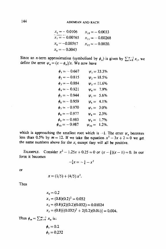
x, = - 0.0106 x,~ = - 0.0033 -- x, = - 0.00765 x,, = - 0.00268

x, = -0.00567 x1* = - 0.0020. x, = - 0.0043

Since an n-term approximation (symbolized by 0,) is given by Cy:i xi, we define the error I,U, = (x - 4,)/x. We now have

$I = - 0.667

#2=-0.815

#3 = - 0.884

lj4 = - 0.92 1

#5 = - 0.944

46 = - 0.959

0, = - 0.970

$8 = - 0.977

q$, = - 0.983 #lo = - 0.987

y, = 33.3%

yz = 18.5%

y3 = 11.6%

y4 = 7.9%

ys = 5.6%

ys = 4.1%

y,= 3.0%

y8 = 2.3%

y9= 1.7% ylo= 1.2%.

which is approaching the smallest root which is -1. The error vC/n becomes less than 0.5% by m = 12. If we take the equation x2 - 3x + 2 = 0 we get the same numbers above for the xi except they will all be positive.

EXAMPLE. Consider x2 - 1.25x + 0.25 = 0 or (x - a)(x - 1) = 0. In our form it becomes

-$x=-+X2

or

Thus

x = (l/5) + (4/5) x2.

x0 = 0.2

x, = (0.8)(0.2)’ = 0.032

x2 = (0.8)(2)(0.2)(0.032) = 0.01024

x3 = (0.8)[(0.032)* + 2(0.2)(0.01)1 = 0.004.

Thus 4, = 2::: x, is:

4, = 0.2

ti2 = 0.232

THE DECOMPOSITION METHOD OF SOLUTION 145

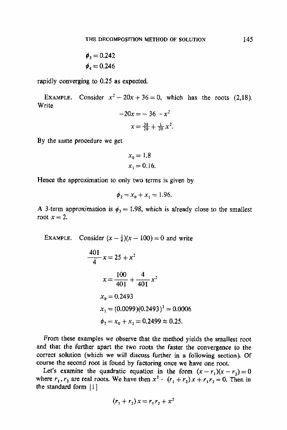
/3 = 0.242

4, = 0.246

rapidly converging to 0.25 as expected.

EXAMPLE. Consider x2 -20x + 36 = 0, which has the roots (2,18). Write

-20x=-36-x2

36 2 x=x+&x.

By the same procedure we get

x0 = 1.8

x, = 0.16.

Hence the approximation to only two terms is given by

#2 =x,, + x1 = 1.96.

A 3-term approximation is #3 = 1.98, which is already close to the smallest root x = 2.

EXAMPLE. Consider (x - 4)(x - 100) = 0 and write

401 4x = 25 +x2

100 4 x=-+.--x*

401 401

xc) = 0.2493

x, = (0.0099)(0.2493)’ = 0.0006

$2 = x, +x1 = 0.2499 % 0.25.

From these examples we observe that the method yields the smallest root and that the further apart the two roots the faster the convergence to the correct solution (which we will discuss further in a following section). Of course the second root is found by factoring once we have one root.

Let’s examine the quadratic equation in the form (x - rr)(x - r2) = 0 where r, , rz are real roots. We have then x2 - (r, + r2) x + r, r2 = 0. Then in the standard form [ 1 ]

(r, + rz) x = r, rz + x2


v2 1 x=---+-x2.

r1 +r2 r1 +r2

Now since x = C,“=. x, and we identify x0 = r, r2/(r, + r2), the x,, I for n = 0, l,..., are given by

1 X n+l =----A,

r1 + r2

or

x=x0+ 2 -L4, n=O rl+r2

where the A,, have already been given for Nx = x2. Since r, r2 = c/a and rl + r2 = -b/a in the standard ax2 + bx + c form, we

have

x = -(c/b) - (a/b) x2

where

x0 = c/b

x1 = (a/b) xi

x2 = WPoxl)

etc.

Note, e.g., that in solving (x-x)(x - 4) = 0 where we have deliberately chosen the 2nd root to be only a little larger than the root rr, we have x2 - (n+4)x+47r=O. Wehave

4n 1 2 x=---t-x 71t4 nt4

so that x0 = 1.76. If we consider (x - z)(x - 10) = 0 we get x0 = 2.39. If we take the second root as 100, x0 = 3.05 and for the second root x = 1000, x0 = 3.13, an error of 0.3% with only the x0 term to obtain the smaller root. Thus the results converge to the desired solution more and more quickly, i.e., for smaller n, as the roots are further apart. In general for (x - r&x - r2) = 0, or x2 - (r, + r2) x + r, r2 = 0, we have the first term

5 r2 x,=-. rl + r2


If rz > rl , we have x,, N rlrz/rz = r, . Since the following terms involving the A,, are divided by the factor I/(r, t rz) or approximately l/r,, the other terms vanish early.

Decimal Roots

Finally, as we have previously stated, the roots are not limited to integers. Consider, for example,

x2-5.15x+2.37=0

5.15x=2.37 +x2

2.37 1 a\ x=5.15+ 5.15 0 -3 A”.

We get immediately

x0 = 0.460

x,=0.0411

x2 = 0.00735.

Thus the 3-term approximation #3 =x,, t x, t x2 = 0.50845. Let’s call this r2. But rl rz = 2.37 hence r, = 2.37/0.50845 = 4.66. The sum of the roots now constitutes a check by comparison with the coefficient of the middle term of the quadratic equation. We observe in doing this an error less than 0.3% and considering we only used a 3-term approximation, the result is excellent.

Complex Roots

If we have complex roots zr, z2 then (x - z,)(x - z2) = 0 or x2 - (z, + zz)x + zlzz = 0. Thus the sum of the roots is the coefficient of the x term and the product of the roots is the constant term. Consider an example with complex roots but real coefficients

x2 - 2x f 2 = 0.

Solving it in the usual manner with decomposition, we have

x=1+fx2=1+ffA,. 0

Therefore we take

x0= 1

148 ADOMIANANDRACH

and obtain immediately

i.e., a diverging series (for a quadratic equation with real coefficients) may’ indicate complex roots. In that case, as complex roots occur in conjugate pairs, e.g., Q + bi and a - bi, their sum is 2a and their product is a2 + b*.

Comparison with the coefficients in the equation shows 2a = 2 or a = 1 and uz + b* = 2, hence b = 1. Therefore the roots are 1 + i and 1 - i.

EXAMPLE. Quadratic equation with complex roots c,, c2 given by (x - c,)(x - c,) = 0 or x2 - (cl + c,) x + clcz = 0 where c,, c, E C, the set of complex numbers. In the standard Adomian decomposition form, we get

x=p++x*

where p = a + $3 and v = y + id can of course be written in terms of real and imaginary components of c,, c,. We write

where

A,=x;

A,=2xoxl

A, = x; + 2x,x,

A, = 2x,x, + 2x,x,

’ The associated equation with different signature, x2 - 2.x - 2 = 0, which does have real roots, also results in a diverging series. This special case has been handled by an ingenious method discussed in Adomian [2], which also solves equations of the form Ny = x such as ey = x, for example.


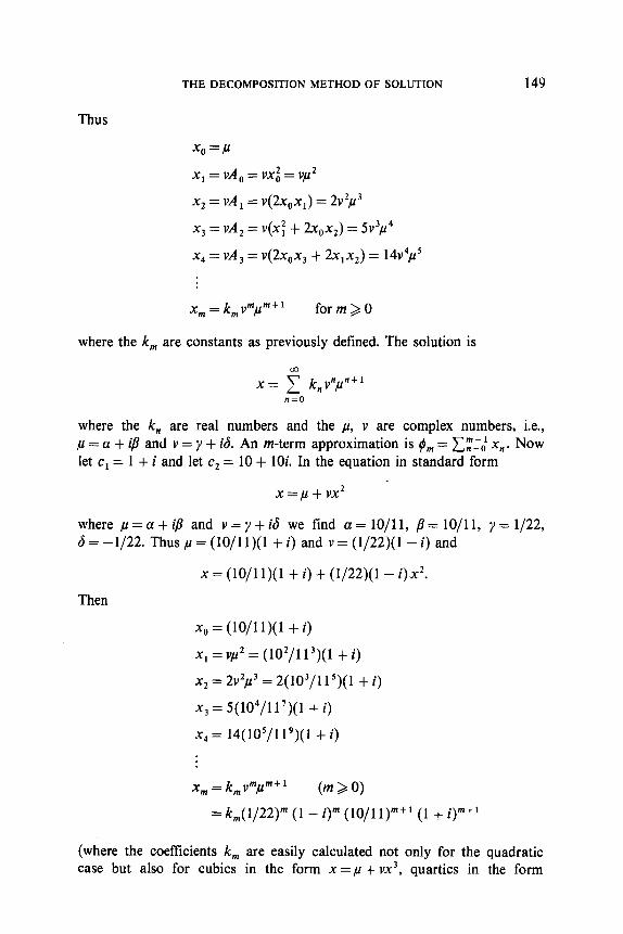
Thus

Xo=P x, = VA, = vx; = v/l2 x2 = VA 1 = v(2x,x,) = 2v5l3 x3 = VA, = v<x; + 2x,x,) = 5v3p4 x4 = VA, = v(2x,x, + 2x,x,) = 14v4p5

x, = k,vm,u”+l for m > 0

where the k, are constants as previously defined. The solution is

x= -f k&d’+’ n=o

where the k, are real numbers and the ,u, v are complex numbers, i.e., ,U = a + i/l and v = y + id. An m-term approximation is 4, = Cf:,’ x,. Now let c, = 1 t i and let c, = 10 t 1Oi. In the equation in standard form

x=p +vx2

where p=a+ifi and v=ytiS we find a=lO/ll, p=lO/ll, y= l/22, 6 = -l/22. Thus ,U = (lO/ll)(l t i) and v = (l/22)(1 -i) and

x=(10/11)(1 ti) t (l/22)(1 -i)x2.

Then

x0 = (10/l l)(l t i)

xi =vp2 = (102/113)(1 + i)

x2 = 2v*p3 = 2(103/l P)(l + i)

x3 = 5(104/117)(1 + i)

x4 = 14(105/119)(1 + i)

x, = k,,,vmjF1 (m 2 0)

= k,(1/22)m (1 -i)” (lO/ll)“‘+ * (1 + i)m+’

(where the coefficients k, are easily calculated not only for the quadratic case but also for cubits in the form x =,u t vx3, quartics in the form


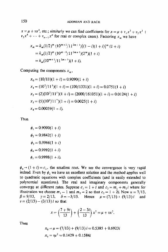
x =p + vx4, etc.; similarly we can find coeffkients for x = ,U + v,x2 + v2x3 + v3x4 + ... + v,_,x” for real or complex cases). Factoring x, we have

x, = k&/2)” (lom+l/l P+‘)[(l - i)(l + i)]” (1 + i)

= k,(1/2)” (lOm+‘/ll *“+‘)(2”)(1 + i)

=k,(10m+1/112m+1)(1 +i).

Computing the components x,,

x0 = (lO/ll)(l + i) = 0.9090(1 + i)

x1= (102/113)(1 +i)=(100/1331)(1 +i)=O.O751(1 +i)

x2 = (2)(10)/l 15)(1 + i) = (2000/161051)(1 t i) = 0.0124(1 t i)

xj= (5)(104/11’)(1 +i)=O.O025(1 +i)

x4 = 0.00059(1 + i).

Thus

II = 0.9090(1 f i)

fb2 = 0.9842(1 + i)

#3 = 0.9966(1 + i)

q+4 = 0.9992(1 + i)

g& = 0.9998(1 i-i).

#,-(I ti)=c,, the smallest root. We see the convergence is very rapid indeed. Even by d2 we have an excellent solution and the method applies well to quadratic equations with complex coeffkients (and is easily extended to polynomial equations). The real and imaginary components generally converge at different rates. Suppose c, = 1 t i and cr = m, t m,i where for illustration we choose m, = 1 and m2 = 2 so that c2 = 1 + 2i. Now a = 7/13, /I= 9/13, y = 2/13, 6 = -3/13. Hence ,u = (7/13) t (9/13) i and v = (2/13) - (3/13) i so that

x= (zig) + (~)x2=pt”x2.

Then x,, =p = (7/13) t (9/13) i = 0.5385 t 0.69231’

x1 = v/i* = 0.1429 + 0.1584~.


x2 = 2v2,u3 = 0.0749 + 0.07 1%

x3 = 5v3p4

x4= 14v4p5

The n-term approximate solutions are:

4, = 0.5385 t 0.69231’

qi2 = 0.6814 t 0.8507i

#3 = 0.7564 t 0.92251’

#,=lti.

It is clear that the imaginary component is converging more rapidly than the real component so we have a differing convergence for the real and imaginary components of complex roots.

II. CUBIC EQUATIONS

Consider now equations of the type z3 +A2z2 t A,z t A, = 0. The z2 term is ordinarily eliminated by substituting z = x -A ,/3 to get an equation in the form x3 - qx - r = 0. Thus, the equation

z3 t 9z2 + 232 + 14 = 0

becomes (substituting z = x - 3)

x3-4x-1=0

whose roots are 2.11, -1.86, -0.254. If we solve this by decomposition we write the equation in the form [ I] -qx = r - x3 or

-4x= l-2

x=--f+p

x=x,+d f An* n=o

152 ADOMIANANDRACH

For this nonlinearity (Nx in Adomian’s notation [ 11)

A, = 3x:x,

A, = 3x:x, + 3x,x;

A, = 3x:x, + 6x,x,x, +x;

A, = 3x:x, + 3x,x; + 6x,x,x, + 3x:x,

A, = 3x:x, + 6x0x,x, + 6x,x,x, + 3x:x, + 3x,x;.

(We caution against simply extrapolating the A,, to higher it. We cannot include the complete generating scheme for any n in this paper. It depends on the actual nonlinearity and is lengthy to discuss so it will be dealt with elsewhere. The objective of this paper is to show applicability to algebraic equations, not to provide a handbook.) Thus x0 = -0.25, x, = +A,,=

14= -a - 0.004, etc. Thus the one-term approximation #i = -0.25, the two- term approximation dz = -0.254, and x, ‘v 0 for an answer to three decimal places so the correct solution is obtained already with )* (again for the smallest root). #3 gives -0.254 with no more change to 3 decimal places. Computing 6 terms gives -0.25410168, which doesn’t change any further to 8 place accuracy.

If we now divide x3 -4x - 1 by x - 0.254, we obtain x2 + 0.254x - 3.9375, which yields the other two roots by either the quadratic formula or the decomposition method.

The equation x3 - 6x2 + 1 lx - 6 = 0 has roots (1,2, 3). Written in the form

6 6 2 1 3 x=n++x -xx

and solving by the decomposition method, it yields x0 = 0.5455, x1 = 0.1475,..., and the solution x = 1 in eight terms.

EXAMPLE. x3 + 4x2 t 8x t 8 = 0 is satisfied by x = -2. Calculating this with appropriate A,, for the x2 and x3 terms, we get

x, = -1.0

x1 = -0.375

x2 = -0.234375

x3 = -0.1640625

x4 = -0.1179199

x5 = -0.0835876.

THEDECOMPOSITIONMETHODOFSOLUTION 153

If we sum these terms we get approximately x = -1.98, which makes us guess x= -2.0 and try it in the equation. (It is interesting to note, however, that we actually have an oscillating convergence. If we sum 10 terms, we get x = -2.0876342, which is a peak departure from x = -2. At 20 terms we have a peak departure in the opposite direction with x = -1.9656587. At 100 terms we have -1.997313.)

EXAMPLE.

x3-6x2+ 11x-6=0

6 6 1 x=II+Mx*-IIx3

,f x,=x,+&f An-+ f B, n=o n-0 n-0

expanding the x2 and x3 terms in our usual polynomials but using A,, and B, to distinguish the two.

x0 = 6/l 1 = 0.5455

x1= (&)A,- (-&) B,= (r)(s) =0.147531

x2 = (&)A, - (+)B, = ('9)(Lo)($) =0.0758160

x3= (+)A*- (+)B,=(+$)(3610)=0.038962

qi, = 0.5455

qh2 = 0.69303 1

#3 = 0.768847

#4 = 0.80780

where 4, -+ 1.0 as n -+ co. We can

then write x3 - (r, + r2 + r3) x2 + (rl r, + rl r3 + r2 r3) x - r, rz r3 = 0,

Q-1 r2r3) ' = (r, r, +

(5 + 5 + r3) r1r3+r2rd+ (r1r2+r,r,+r,r,)XZ

1

- (rl 3 + rl r3 + r2 r3) X3


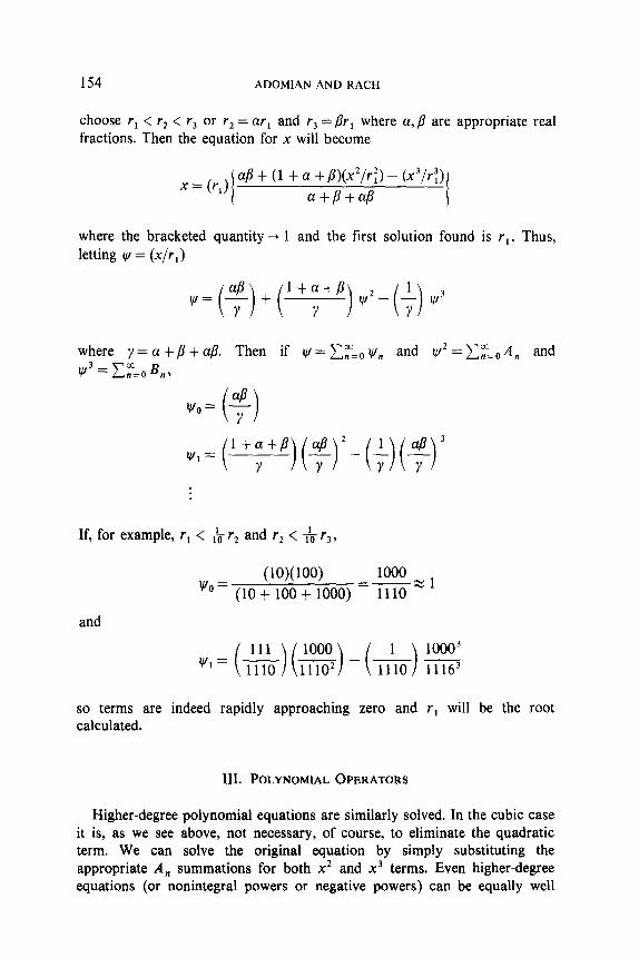
choose rl < r2 < r3 or r2 = ar, and r3 = pr, where a, /3 are appropriate real fractions. Then the equation for x will become

x=(r1) / aP + (1 t a t B)(x*/ri) - (x’lr3

atptap I

where the bracketed quantity + 1 and the first solution found is rl . Thus, letting w = (x/r,)

where y=at/?+a/?. Then if w=C~=~W,, and IJI’=C~=~A,, and w3 = C:=o B, 3

4 wo= - ( 1 Y

If, for example, ri < + r2 and r2 < h r3,

(lO)( 100) 1000 w”= (lo+ 100 + 1000) =XP l

and

v1=(&)($$)-(&J%

so terms are indeed rapidly approaching zero and rl will be the root calculated.

III. POLYNOMIAL OPERATORS

Higher-degree polynomial equations are similarly solved. In the cubic case it is, as we see above, not necessary, of course, to eliminate the quadratic term. We can solve the original equation by simply substituting the appropriate A,, summations for both x2 and x3 terms. Even higher-degree equations (or nonintegral powers or negative powers) can be equally well


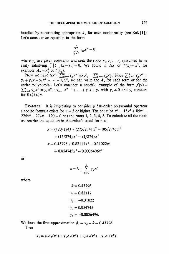
handled by substituting appropriate A, for each nonlinearity (see Ref. [ 11). Let’s consider an equation in the form

i y,x’=O u=O

where y,, are given constants and seek the roots rl, r2,..., r, (assumed to be real) satisfying l-I:=1 (x - r,) = 0. We found if Nx or f(x) = x2, for example, A, = xi or f(x,).

Now we have Nx=C:=, yrxM so A,= ~~=oy,x~. Since c:=. y,,x’ = yo + y,x + y*x* + .** + yp”, we can write the A, for each term or for the entire polynomial. Let’s consider a specific example of the form f(x) = c;=o yrrxfl = ynx” + yn-IX”-’ + . . . + y,x + y. with y, # 0 and yi constant for 0 < i < n.

EXAMPLE. It is interesting to consider a Sth-order polynomial operator since no formula exists for n = 5 or higher. The equation x5 - 15x4 + 85x3 - 225x* + 274x - 120 = 0 has the roots 1, 2, 3, 4, 5. To calculate all the roots we rewrite the equation in Adomian’s usual form as

x = (120/274) + (225/274) x2 - (85/274) x3

+ (15/274) x4 - (l/274) x5

x = 0.43796 + 0.82117~~ -0.31022x3

t 0.054745x4 - 0.0036496x5

or

where

x=k+ i Ynx” n=2

k = 0.43796

y,=O.82117

y3 = -0.3 1022

y4 = 0.054745

y5 = -0.0036496.

We have the first approximation $r = x0 = k = 0.43796. Then

x,= y2A,(x2)+ yJ,(x3) + Y4Ao(X4) + Y,Ao(-e.


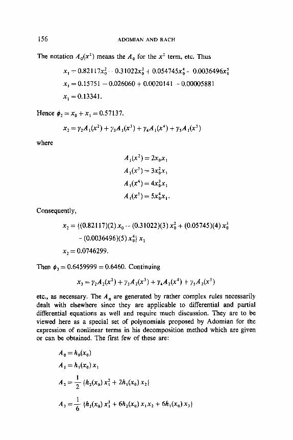
The notation A,(x2) means the A, for the x2 term, etc. Thus

x1 = 0.82117x; - 0.3 1022x; + O.O54745xQ, - 0.0036496x;

x, = 0.15751- 0.026060 + 0.0020141 - 0.00005881

x, = 0.13341.

Hence #* =x,, +x, = 0.57137.

x2 = Y2A,(X2) + Y3A,(X3) f Y4Al(X4) + Y54(X5)

where

A ,(x2) = 2x,x,

A,(X3) = 3x:x,

A 1(x”) = 4x:x,

A 1(x”) = 5x:x, *

Consequently,

x2 = {(0.82117)(2) x,, - (0.3 1022)(3) x’o + (0.05745)(4) xi

- (0.0036496)(5) xi} x,

x2 = 0.0746299.

Then & = 0.6459999 = 0.6460. Continuing

x3 = Y2A2(X2) + Y3A2(X3) + y4A2(x4) + hA2(x5)

etc., as necessary. The A, are generated by rather complex rules necessarily dealt with elsewhere since they are applicable to differential and partial differential equations as well and require much discussion. They are to be viewed here as a special set of polynomials proposed by Adomian for the expression of nonlinear terms in his decomposition method which are given or can be obtained. The first few of these are:

A, = M-d

A, = Wdx,

A3 = + {h3(xJ xi + 6h2(xJ ~1x2 + 6h,(x,) ~3 ]


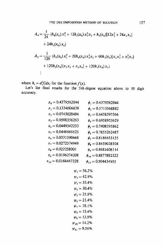
Al=& {h&J x: t 12@,) x:x, t &(-q,)[ 12x: t 24x,x,]

A,= & IUJx: + 2%(x0)4x, + 6%Wl+4 +x:-d

where hi = dif/dxi for the function f(x). Let’s list final results for the Sth-degree equation above to IO digit

accuracy.

x, = 0.4379562044

x, = 0.1334006838

x, = 0.0745028484

x3 = 0.0500356263

x4 = 0.0449342233

x5 = 0.0446966625

x6 = 0.0331390668

x, = 0.0272374949

x8 = 0.022258001

x9 = 0.0196274208

xl0 = 0.0166467228

I, = 0.4379562044

ti2 = 0.5713568882

#3 = 0.6458597366

#4 = 0.6958953629

$, = 0.7408295862

q& = 0.7855262487

4, = 0.8186653155

& = 0.8459028 104

fd9 = 0.8681608114

#,,, = 0.8877882322

#,I = 0.904434955

y1 = 56.2%

y2 = 42.9%

l/f, = 35.4%

ly4 = 30.4%

ys = 25.9%

‘y, = 21.4%

v, = 18.1%

l/l8 = 15.4%

qY9 = 13.9% I//,() = 11.2%

I/, 1 = 9.56%


The error v/ decreases gradually to less than 10% by vll but it can easily be carried further by computer. The convergence for inversion in this case of a quintic operator is relatively poor because of the greater number of more closely spaced roots and the case of equal roots will be the poorest case.

Forf(x) = xk where k is an integer 22, let’s write h, = d”f,dx” for n > 0. (We will write h,(x,) for (d”f/dx”)(,=, for the computation of the A,.) Then for Xk.

h,=xk

h =kxk-’ 1

h,=k(k-I)..+-n+I)xk-“= Xk-n

where (,“) = k!/(k - n)!. Consequently, the A, for f(x) = xk are given by

A,=x;

~=](;)x:-~/x,

A2=f-](:)x~-21x~+](~)x~-~~x*

A3=~~(:)x:-3~~:+~(;)x:-2~x~x2+~(;)x~-~~x3

A=& ](~)x~-‘j+~](~)x~-‘~x;x2

+](~)x~-2[[tx:+x~x3~+](:)x:‘lx4

x [XIX: +x:x3] + [x2x3+x,x4j+ 1 (;) x:-‘/ x5’

We observe that the subscripts for A, always add to n and the superscripts of the x,.‘s always add to k.

The above work will yield the lowest root, or 1, reducing the equation to a 4th power then the root 2, etc. We can do the problem more rapidly as follows.


Let’s write a general polynomial in x with constant nonzero coefficients.

f(x)= ,jkyiXi=y*xk t .‘* +yO*

Now

h, = i yixi i=k

h, = ‘s iyixi-’ i=k

yi+ (k>n)

(k=n)

h k+l ==0 or h, = 0 for n > k.

The A,, can now be given

A, = c yix; i=k


++ I($& YiXY jw: +x:x31 +]jJ (:)y~Xh-‘/~X*X3+X,X4)+] i ( :) Yixbl! x5

i=k i=k

etc.

from which polynomial equations can be solved more rapidly than with individual substitutions for the various powers as we did earlier in this paper.

Negative powers. Consider an example like x = 2 + x-* or the more general form

x=k+x-m.

We write

2 x,=k+ f A, n=O n=O

with xo=k andx,=A,-, for n> 1. Then

x5 = A, = $-m(m + l)(m + 2)(m + 3) x,(~+~)x’: - fm(m + 1)

x(m+2)x, (m+3)X;X2 + m(m + l)x,‘“+“[;x: +x,x,]

- m;(m+l)x4.

Ifk=2andm=2,thenxo=2and

x,=2-*=0.25

x2 = -2(2) -3 (0.25) = - 0.0625

x3 = +(2)(3)(2)-4(0.25)2 - (2)(2)-3 (-0.0625) = 0.02734375

x4 = -0.0146484375

x5 = -0.0087280273.


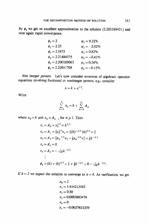
By #6 we get an excellent approximation to the solution (2.205569431) and note again rapid convergence.

11=2 l/f, = 9.32%

(b2 = 2.25 wz = -2.02%

& = 2.1875 ty3 = 0.82%

#4 = 2.21484375 y4 = -0.42%

#5 = 2.200189063 w5 = 0.24% I& = 2.2089 1709 lya = -0.15%

Non integer powers. Let’s now consider inversion of algebraic operator equations involving fractional or noninteger powers, e.g., consider

x = k t xl”.

Write

f x,=k+ f A, n=O n=O

where x0 = k and x, = A,- I for n > 1. Then

x1 zz A, = x;‘~ = k’j2

x2 =A, = fx;“x, = f(k)-‘/* @)‘I* =)

x3 =A, = ix-‘f2x2 _ +x,3f2X; = $-l/2 2 0

X4=A3=0

~~=A~=-&k-~f~

4, = (k) t (k)“2 + 4 f {k-‘i2 $0 - -&k-3f2.

If k = 2 we expect the solution to converge to x = 4. As verification, we get

x0 = 2

x1 = 1.414213562

x2 = 0.50

x3 = 0.0883883476

xq = 0

x5 = -0.0027621359

162 ADOMIANANDRACH

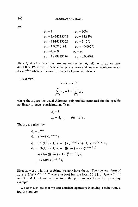
and

#1=2 ‘yl = 50%

yb2 = 3.414213562 w2 = 14.65%

4, = 3.914213562 ty3 = 2.15%

#4 = 4.00260191 y4 = -0.065%

95 = 64 + 0 ws = w4

& = 3.999839774 W6 = 0.0040%.

Thus OS is an excellent approximation (in fact #4 is!). With OS we have 4/1000 of 1% error. Let’s be more general now and consider nonlinear terms Nx = x’fm where m belongs to the set of positive integers.

EXAMPLE.

x=k+x”“’ 00

-S x,=kt f A, “50 II=0

where the A, are the usual Adomian polynomials generated for the specific nonlinearity under consideration. Then

x0 = k

x, =An-l for n>l.

The A, are given by

A, =x;“” A, = (l/m) xr’m)-‘x,

A, = 1/2(l/m)((l/m) - 1)x:‘“‘-*x: t (l/m)x~‘“‘-‘x,

A, = 1/6(l/m)((l/m) - l)((l/m) - ~)x~‘“‘-~x:

+ (l/m)((l/m) - 1)xb”m’-2x,x,

+ (l/rn)~~‘I~)-~x~

Since x, = A, _ i in this problem, we now have the x, . Their general form of x, is a( l/m) kc”/“)-“+ ‘) where a(l/m) has the form xi nj oi(l/m -pj). If m = 2 and k = 2 we get precisely the previous results in the preceding example.

We now also see that we can consider operators involving a cube root, a fourth root, etc.


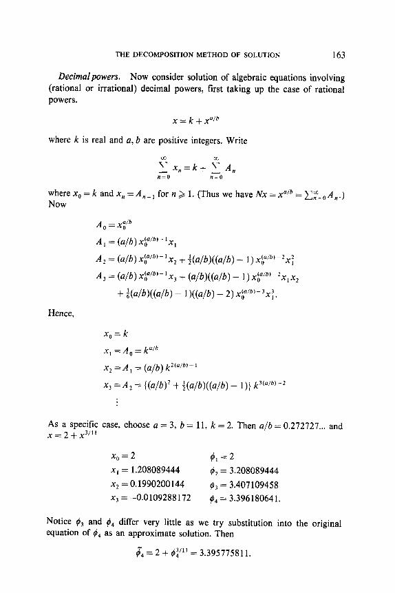
Decimalpowers. Now consider solution of algebraic equations involving (rational or irrational) decimal powers, first taking up the case of rational powers.

x = k t xalb

where k is real and a, b are positive integers. Write

5 x,=k+ ? A, n=O Jl=O

wherex,=kandx,=A,-, forn~l.(ThuswehaveA!x=xa’b=~~~oA,,.) Now

Ao=xfb

A, = (a/b) xp’b)-‘xl

A 2 = (a/b) xr’“‘- ’ x2 t i(a/b)((a/b) - 1) x~‘~)-‘x~

A, = (a/b) xrlb)-’ x3 t (a/b)((a/b) - 1) x~‘~)-~x,x~

t i(a/b)((a/b) - l)((a/b) - 2) x~‘~)-~x:.

Hence,

x0 = k

x, = A, = kalb

x2 = A 1 = (a/b) k2(a’b)- I

x3 = A, = {(a/b)* t i(a/b)((a/b) - l)} k3(‘lb’-*

As a specific case, choose a = 3, b = 11, k = 2. Then a/b = 0.272727... and x=2+x3’”

x0 = 2 f4=2

x1 = 1.208089444 @2 = 3.208089444

x2 = 0.1990200144 9, = 3.407109458

x3 = -0.0109288172 qb4 = 3.396180641.

Notice 4x and #4 differ very little as we try substitution into the original equation of #4 as an approximate solution. Then

& = 2 t #:“l = 3.395775811.


We see $d is very close to $4, differing by about 0.01%. (We have defined &,-k+#, ‘lb to see if the approximate solution satisfies the original equation.)

Now we consider the case of irrational powers. Write

x=k-xY

letting k be real and y an irrational number such as e or 7~. Now

wherex,=kandx,=-A,-, fern> 1. SinceNx=xY=C~zoAn,

A,=$

A, = yxoy-1x,

A,=jx-‘x,+Qy(y- l)x;-‘x:

A, = yx’xoy-‘x~ + y(y - l)x,y-*x,x,

+ $y(y- l)(y - 2)x:-3x:.

Now the components x, of the solution x = CFEo x, can be computed

x0 = k

x, = -kY

x2 = yk*Y-’

x3 = - {y* + +y(y - l)} k3y-2

x4 = {y*(y - 1) + +y(y - l)(y - 2) + y3 + +“(y - l)} k4y-3.

For a specific example we now choose k = l/z and y = 7c

x = (l/n) - x*

(letting n = 3.1415927 and l/z = 0.3 183099 for the computation). We get x = 0.296736 which is within a hundredth of 1%.

Random algebraic equations. The treatment of algebraic equations by the decomposition method suggests further generalization to random algebraic equations. Such equations, with random coefficients, arise in engineering, physics, and statistics whenever random errors are involved. Random matrices* too are found in finite-dimensional approximation models

2 Application of the decomposition method also solves equations with random matrix operators. See [5-71.


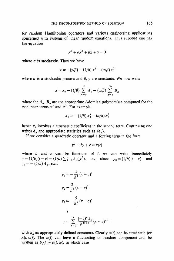
for random Hamiltonian operators and various engineering applications concerned with systems of linear random equations. Thus suppose one has the equation

x3 +ax* +px+y=o

where a is stochastic. Then we have

x = -(r/P> - (VP) x3 - WP> x2

where a is a stochastic process and /3, y are constants. We now write

where the A,, B, are the appropriate Adomian polynomials computed for the nonlinear terms x3 and x2. For example,

hence x1 involves a stochastic coefficient in the second term. Continuing one writes 4, and appropriate statistics such as (4,).

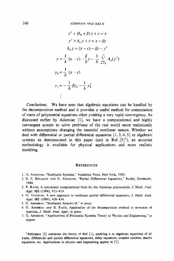
If we consider a quadratic operator and a forcing term in the form

y* -I- by + c = x(t)

where b and c can be functions of t, we can write immediately y = (l/b)(t - c) - (l/b) CzEoA,(y2), or, since y, = (l/b)(t - c) and y, = - (l/b)A,, etc.,

y1 = - ; (x - c)’

y, = ; (x - c)”

y, = - $ (x - c)”

y= -f w”k”(x-c)“-l

n=O bhtl

with k, as appropriately defined constants. Clearly x(t) can be stochastic (or x(t, 0)). The b(t) can have a fluctuating or random component and be written as bO(t) + P(t, o), in which case

166 ADOMIANAND RACH

Conclusions. We have seen that algebraic equations can be handled by the decomposition method and it provides a useful method for computation of roots of polynomial equations often yielding a very rapid convergence. As discussed earlier by Adomian [ 11, we have a computational and highly convergent system to solve problems of the real world more realistically without assumptions changing the essential nonlinear nature. Whether we deal with differential or partial differential equations [ 1,2,4,5] or algebraic systems as demonstrated in this paper (and in Ref. [513), an accurate methodology is available for physical applications and more realistic modeling.

REFERENCES

1. G. ADOMIAN, “Stochastic Systems,” Academic Press, New York, 1983. 2. R. E. BELLMAN AND G. ADOMIAN, “Partial Differential Equations,” Reidel, Dordrecht,

1984. 3. R. RACH, A convenient computational form for the Adomian polynomials, J. Math. Anal.

Apple 102 (1984), 415-419. 4. G. ADOMIAN, A new approach to nonlinear partial differential equations, J. Math. Anal.

Appl. 102 (1984),42&434. 5. G. ADOMIAN, “Stochastic Systems II,” in press. 6. G. ADOMIAN AND R. RACH, Application of the decomposition method to inversion of

matrices, J. Math. Anal. Appl., in press. 7. G. ADOMIAN, “Applications of Stochastic Systems Theory to Physics and Engineering,” to

appear.

’ Reference [5] continues the theory of Ref. [ 11, applying it to algebraic equations of all kinds, differential and partial differential equations, delay equations, coupled systems, matrix equations, etc. Applications to physics and engineering appear in [7].

on the solution of algebraic equations by the …on the solution of algebraic equations by the...

Documents