on the solution of the de saint-venant’s problem …on the solution of the de saint-venant’s...
TRANSCRIPT
On the solution of the de Saint-Venant’s problem and its limitations
Giuseppe Vairo
Università dgli Studi di Roma “Tor Vergata”Dipartimento di Ingegneria Civile
UniversitUniversitàà degli Studi di Paviadegli Studi di PaviaDipertimento di Meccanica StrutturaleDipertimento di Meccanica Strutturale
7th November, 20087th November, 2008

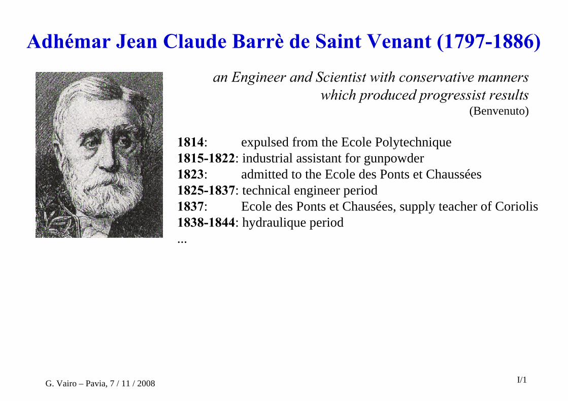
Adhémar Jean Claude Barrè de Saint Venant (1797-1886)an Engineer and Scientist with conservative manners
which produced progressist results (Benvenuto)
G. Vairo – Pavia, 7 / 11 / 2008 I/1
Adhémar Jean Claude Barrè de Saint Venant (1797-1886)an Engineer and Scientist with conservative manners
which produced progressist results (Benvenuto)
G. Vairo – Pavia, 7 / 11 / 2008 I/1
1814: expulsed from the Ecole Polytechnique1815-1822: industrial assistant for gunpowder1823: admitted to the Ecole des Ponts et Chaussées1825-1837: technical engineer period1837: Ecole des Ponts et Chausées, supply teacher of Coriolis1838-1844: hydraulique period...
... the use of the mathematics will stop attracting reproaches if one places them in their real limits. The pure calculus is simply a tool... Mechanics add some physical principles, experimentally well-founded, but leave the validation task for the results to particular experiences . Results of mathematics and calculus are not unfailing “oracles”... but they are simply indications, precious, but only indications which reduce the field of the “instinctive evaluation”...

De SaintDe Saint--Venant, A. BarrVenant, A. Barrèè, M, Méémoire sur la torsion des prismes. Mmoire sur la torsion des prismes. Méémoires des Savants moires des Savants ééntrangers Acad. Sci. Paris 14 (1855), 223ntrangers Acad. Sci. Paris 14 (1855), 223--560.560.
De SaintDe Saint--Venant, A. BarrVenant, A. Barréé, M, Méémoire sur la flexion des prismes. J. Math. Liouville 1 moire sur la flexion des prismes. J. Math. Liouville 1 (1856), 89(1856), 89--189.189.
He resolved in a not-properly general way a problem addressed by Lamè (1846-1858): the problem of the elastic equilibrium for right prisms acted upon only by tractions on their end-sections
That solution, although not general, gives a fundamental contribution to engineering technical problems
Adhémar Jean Claude Barrè de Saint Venant (1797-1886)
G. Vairo – Pavia, 7 / 11 / 2008 I/2
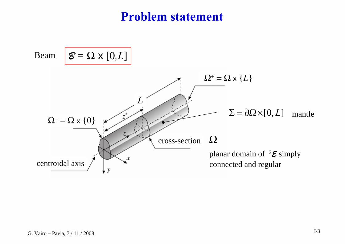
Ωplanar domain of 2E simply connected and regular
B = Ω x [0,L]
L
Ω+ = Ω x {L}
Ω− = Ω x {0}],0[ L×Ω∂=Σ mantle
Problem statement
Beam
cross-section
centroidal axis
G. Vairo – Pavia, 7 / 11 / 2008 I/3

B is free (not constrained)it is not acted upon by volume forces and tractions on Σit is acted upon only by tractions on Ω+/- (denoted by p+/-)
Problem statement
G. Vairo – Pavia, 7 / 11 / 2008 I/4

B is free (not constrained)it is not acted upon by volume forces and tractions on Σit is acted upon only by tractions on Ω+/- (denoted by p+/-)
B is in equilibrium
0prpr
0pp
=×+×
=+
∫∫∫
−+ Ω
−
Ω
+
Ω
−+
dada
da
Bin div 0σ =
−+−+−+Σ
Ω=⋅
Σ=⋅/// su
su
pnσ
0nσ
Problem statement
G. Vairo – Pavia, 7 / 11 / 2008 I/4

The beam is assumed to be homogeneous and comprising isotropic linearly-elastic material
IσσεIεεσ
)( tr/ )2/(1 ) tr( 2EG
Gν−=
λ+=
)21)(1( ,
)1(2 ν−ν+ν=λ
ν+= EEG
Compatibility
0ε Rot Rot =
Problem statement
G. Vairo – Pavia, 7 / 11 / 2008 I/5

Existence Existence UniquenessUniqueness
KirchhoffFichera, ...
Fichera G., Existence Theorem in Elasticity. In: S Flugge (ed.): Hebuch der Physik, Be Vla/2. Springer-Verlag, Berlin 1972.
G. Vairo – Pavia, 7 / 11 / 2008 I/6

∫
∫
∫
∫
∫
∫
Ω
−+−+−+
Ω
−+−+
Ω
−+−+
Ω
−+−+
Ω
−+−+
Ω
−+−+
−=
−=
=
=
=
=
daypxpM
daxpM
daypM
dapT
dapT
dapN
xyt
zy
zx
yy
xx
z
)( ///
//
//
//
//
//
∫
∫
∫
∫
∫
∫
Ω
Ω
Ω
Ω
Ω
Ω
τ−τ=
σ−=
σ=
τ=
τ=
σ=
dayxzM
daxzM
dayzM
dazT
dazT
dazN
xzyzt
zy
zx
yzy
xzx
z
)()(
)(
)(
)(
)(
)(−+−+−+
Σ
Ω=⋅
Σ=⋅/// su
su
pnσ
0nσ
The problem with weak boundary conditions
generalized internal forces
G. Vairo – Pavia, 7 / 11 / 2008 I/7
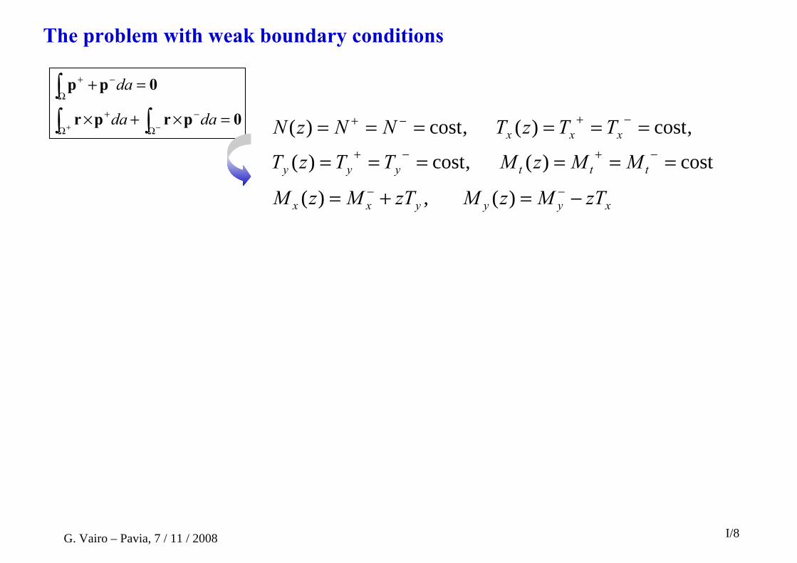
xyyyxx
tttyyy
xxx
zTMzMzTMzM
MMzMTTzT
TTzTNNzN
−=+=
======
======
−−
−+−+
−+−+
)( ,)(
cost)( ,cost)(
,cost)( ,cost)(
The problem with weak boundary conditions
0prpr
0pp
=×+×
=+
∫∫∫
−+ Ω
−
Ω
+
Ω
−+
dada
da
G. Vairo – Pavia, 7 / 11 / 2008 I/8
xyyyxx
tttyyy
xxx
zTMzMzTMzM
MMzMTTzT
TTzTNNzN
−=+=
======
======
−−
−+−+
−+−+
)( ,)(
cost)( ,cost)(
,cost)( ,cost)(
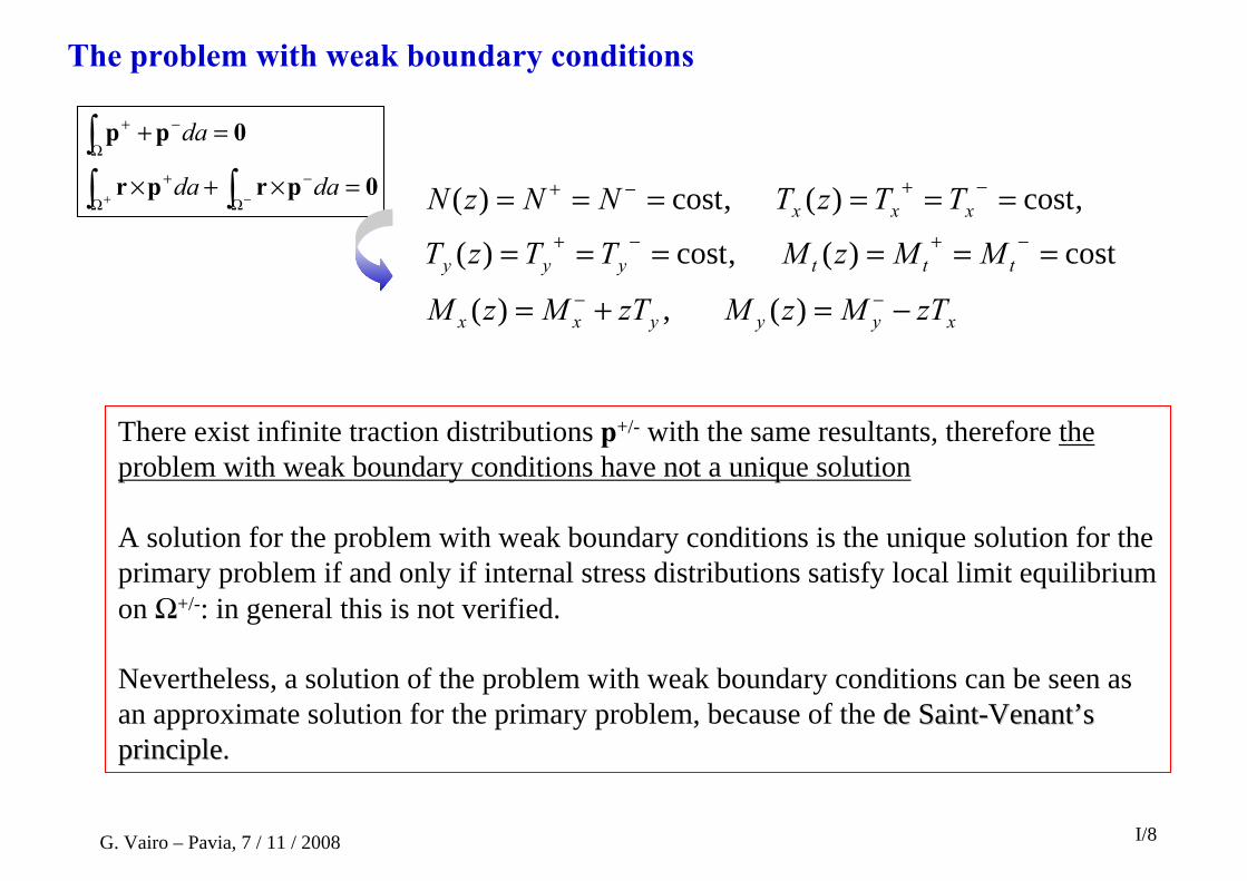
There exist infinite traction distributions p+/- with the same resultants, therefore the problem with weak boundary conditions have not a unique solution
A solution for the problem with weak boundary conditions is the unique solution for the primary problem if and only if internal stress distributions satisfy local limit equilibrium on Ω+/-: in general this is not verified.
Nevertheless, a solution of the problem with weak boundary conditions can be seen as an approximate solution for the primary problem, because of the de Saintde Saint--VenantVenant’’s s principleprinciple.
The problem with weak boundary conditions
0prpr
0pp
=×+×
=+
∫∫∫
−+ Ω
−
Ω
+
Ω
−+
dada
da
G. Vairo – Pavia, 7 / 11 / 2008 I/8

Let the right cylinder B be loaded only on the end-section Ω+ (that is p- = 0) with a self-equilibrated distribution (that is N+=T+=M+=0). Let p+ be sufficiently regular (e.g., square summable on Ω). Let σ and ε the solution of the primary de Saint-Venant’s problem (local limit equilibrium satisfied on the end-sections). Let be Bz = Ω x [0, z]and let U(z) be the strain energy related to Bz:
Then, for every constant 0 < l < L there exixts a constant C > 0(generally depending on L, Ω, E, ν) such that
Toupin R.A.: Saint Venant’s principio. Arch. Rat. Mech. Anal. 18 (1965), 83-96.
In other words: the strain energy for a right cylinder loaded In other words: the strain energy for a right cylinder loaded only on one endonly on one end--sections with a selfsections with a self--equilibrated traction equilibrated traction distribution exponentially decays along the beam axis, when distribution exponentially decays along the beam axis, when the distance from the acted endthe distance from the acted end--section increases.section increases.
de Saint-Venant’s principle
dvzUz
21)( ∫ ⋅=
B
εσ
lLzCzlLLUzU −≤≤−−−≤ 0 ),/)(exp()()(
!G. Vairo – Pavia, 7 / 11 / 2008 I/9

de Saint-Venant’s principle
for compact crossfor compact cross--sections, an effective decay distance from sections, an effective decay distance from the loaded endthe loaded end--section has the same of order of magnitude of section has the same of order of magnitude of an equivalent radius for an equivalent radius for ΩΩ
zF
-F
d
d≈
U(z)/U(L) 1
0.03
G. Vairo – Pavia, 7 / 11 / 2008 I/10
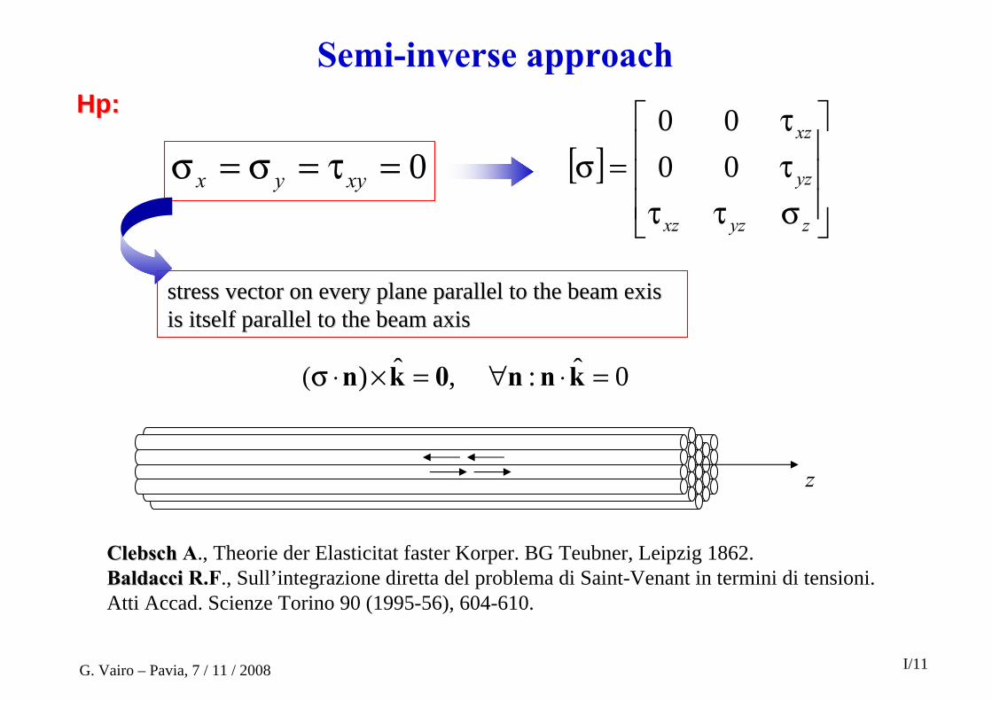
ClebschClebsch A., Theorie der Elasticitat faster Korper. BG Teubner, Leipzig 1862.BaldacciBaldacci R.F., Sull’integrazione diretta del problema di Saint-Venant in termini di tensioni. Atti Accad. Scienze Torino 90 (1995-56), 604-610.
Semi-inverse approachHp:Hp:
0=τ=σ=σ xyyx [ ]⎥⎥⎥
⎦
⎤
⎢⎢⎢
⎣
⎡
σττττ
=
zyzxz
yz
xz
0000
σ
stress vector on every plane parallel to the beam exis stress vector on every plane parallel to the beam exis is itself parallel to the beam axisis itself parallel to the beam axis
0ˆ: ,ˆ) =⋅∀=×⋅ knn0kn(σ
z
G. Vairo – Pavia, 7 / 11 / 2008 I/11

Semi-inverse approach
Bin div 0σ =0 div
),(ˆˆ
/ =σ+
=τ+τ=
zz
zyzx yx
τ
ττ jiin B
Σ=⋅ Σ su 0nσ 0=τ+τ=⋅ yzyxzx nnnτ
Iσσε )( tr/ )2/(1 EG ν−=
0ε Rot Rot =
xzzyyzxxzy
yzzxyzxxzy
xyzzzzyyzxxz
////
////
////
)(
)(
0
σν−=τ−τ
σν=τ−τ
=σ=σ=σ=σ
in B
)1/( ν+ν=ν
Ω∂su
G. Vairo – Pavia, 7 / 11 / 2008 I/12

yI
zMx
IzM
ANy
IzTM
xI
zTMAN
ybxbzyaxaa
x
x
y
y
x
yx
y
xy
z
)()(
)( 2121
+−=+
+−
−=
=+−++=σ−−
ybxb 21 div +=τ
cxbyb +−ν=⋅ )(ˆ)(Rot 21kτΩsu
0=τ+τ=⋅ yzyxzx nnnτ Ω∂su
Semi-inverse approach
G. Vairo – Pavia, 7 / 11 / 2008 I/13

ybxb 21 div +=τcxbyb +−ν=⋅ )(ˆ)(Rot 21kτ
Ωsu
0=τ+τ=⋅ yzyxzx nnnτ Ω∂su
τ+τ=τ 0
])([21
])([21
222
221
cxxyb
cyyxb
zy
zx
+ν−=τ
−ν−=τ
Ω∂=⋅
Ω⎩⎨⎧
=⋅=
su 0
su 0ˆ)(Rot
0 div
0
0
0
0
nτkτ
τ:τ
BaldacciBaldacci R.F., Sull’integrazione diretta del problema di Saint-Venant in termini di tensioni. Atti Accad. Scienze Torino 90 (1995-56), 604-610.
Semi-inverse approach
G. Vairo – Pavia, 7 / 11 / 2008 I/14

Ω∂=⋅
Ω⎩⎨⎧
=⋅=
su 0
su 0ˆ)(Rot
0 div
0
0
0
0
nτkτ
τ:τ
Ψ∇=Ψ∃ 0 ),( τ:yx
Ω∂⋅−=⋅Ψ∇Ω=Ψ∇
su su 02
nτn
well-posed NeumannNeumann--DiniDini problem
Semi-inverse approach
G. Vairo – Pavia, 7 / 11 / 2008 I/15
Ω∂=⋅
Ω⎩⎨⎧
=⋅=
su 0
su 0ˆ)(Rot
0 div
0
0
0
0
nτkτ
τ:τ
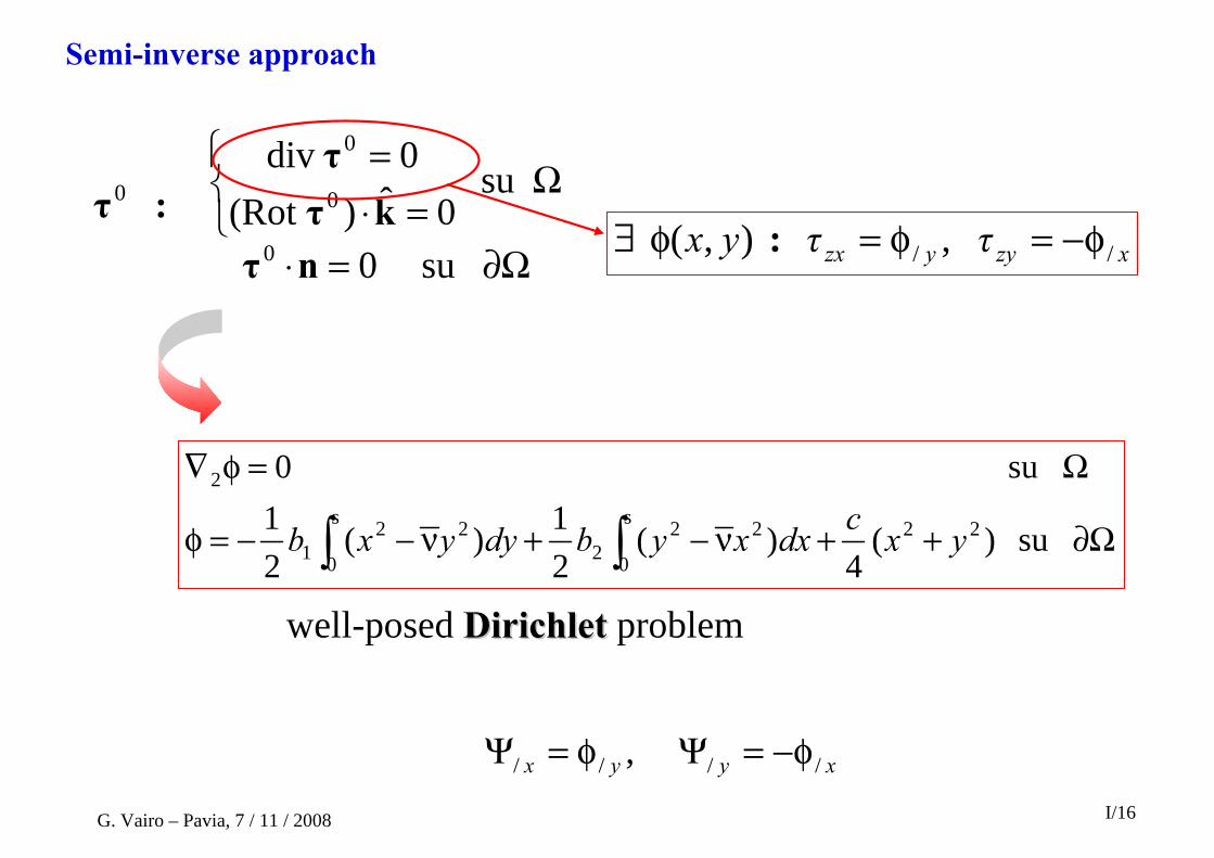
xzyyzx ττyx // , ),( φ−=φ=φ∃ :
Ω∂++ν−+ν−−=φ
Ω=φ∇
∫∫ su )( 4
)(21)(
21
su 0
22s
0
222
s
0
221
2
yxcdxxybdyyxb
well-posed DirichletDirichlet problem
Semi-inverse approach
xyyx //// , φ−=Ψφ=Ψ
G. Vairo – Pavia, 7 / 11 / 2008 I/16
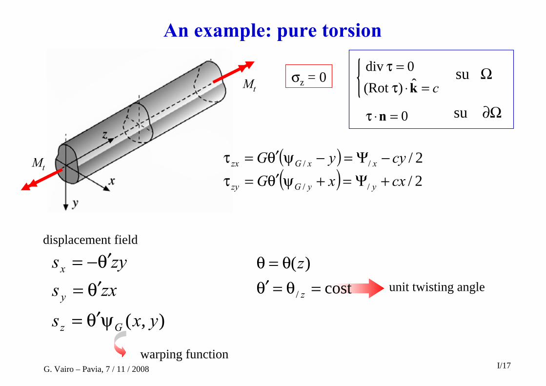
An example: pure torsion
Mt
Mt
0 div =τc=⋅ k)(Rot τ
Ωsu
0=⋅nτ Ω∂su
σz = 0
( )( ) 2/
2/
//
//
cxxGcyyG
yyGzy
xxGzx
+Ψ=+ψθ′=τ−Ψ=−ψθ′=τ
),( yxs
zxszys
Gz
y
x
ψθ′=
θ′=θ′−=
displacement field
cost)(
/ =θ=θ′θ=θ
z
zunit twisting angle
warping functionG. Vairo – Pavia, 7 / 11 / 2008 I/17

Limitations and extension to real casesIn real cases:
• constraints• volume forces• forces on the mantle and not only on the end-sections (also concentrated)• the beam cross-section can be not constant along the beam axis• the beam axis may be curve
decay regions
d
d2≈
G. Vairo – Pavia, 7 / 11 / 2008 I/18
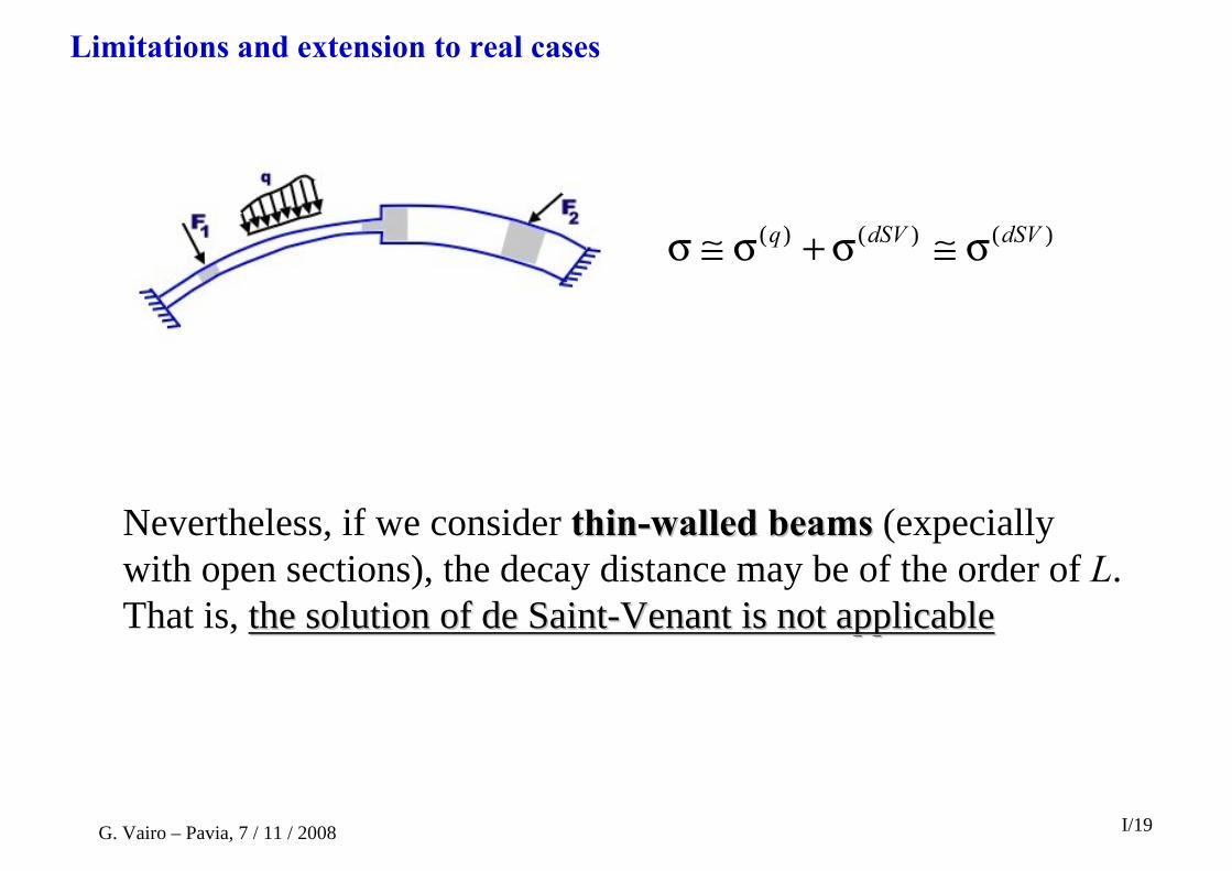
Limitations and extension to real cases
)()()( dSVdSVq σ≅σ+σ≅σ
Nevertheless, if we consider thinthin--walled beamswalled beams (expecially with open sections), the decay distance may be of the order of L. That is, the solution of de Saintthe solution of de Saint--Venant is not applicableVenant is not applicable
G. Vairo – Pavia, 7 / 11 / 2008 I/19
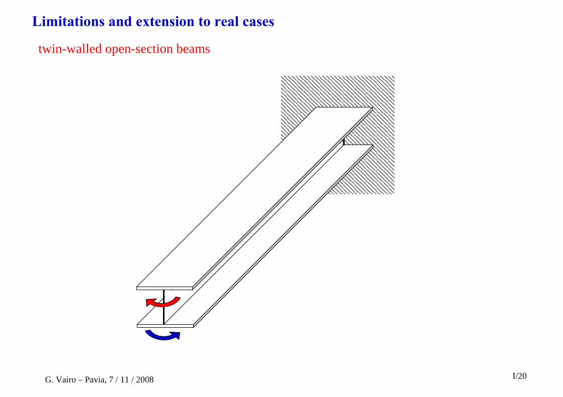
Limitations and extension to real cases
twin-walled open-section beams
G. Vairo – Pavia, 7 / 11 / 2008 I/20
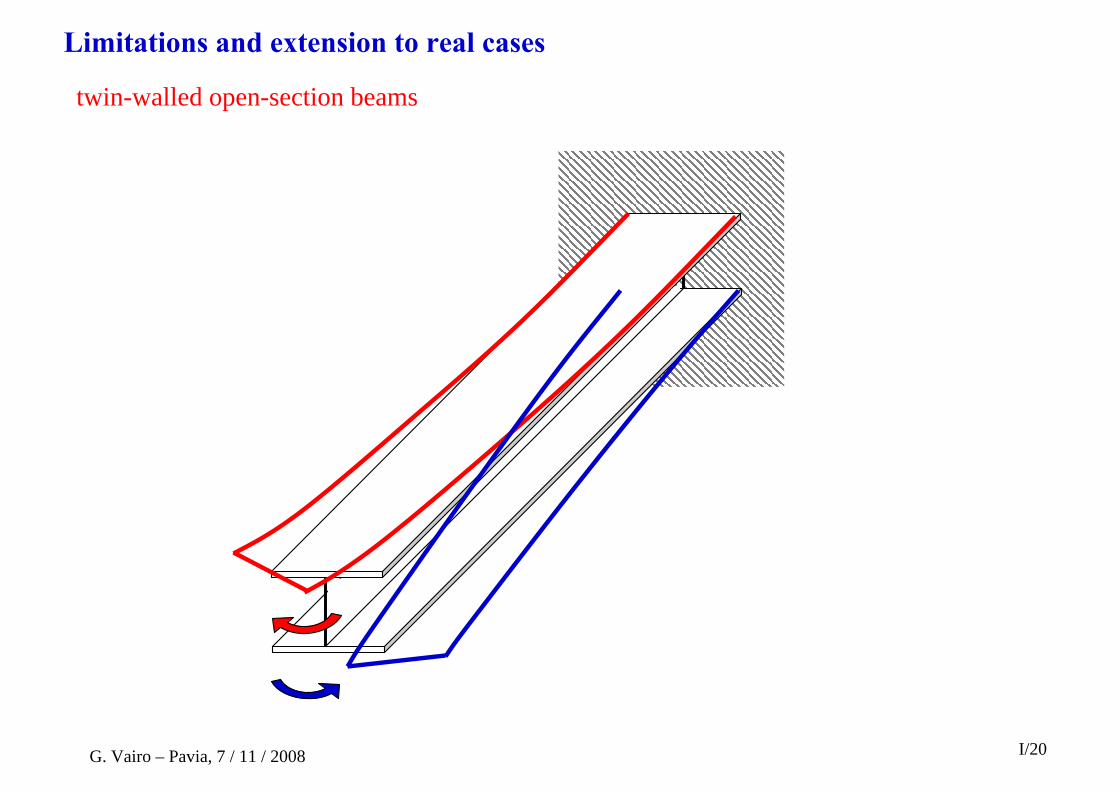
Limitations and extension to real cases
twin-walled open-section beams
G. Vairo – Pavia, 7 / 11 / 2008 I/20

Limitations and extension to real cases
In general, thinIn general, thin--walled beams needs walled beams needs treatments different from those treatments different from those
adopted for classical rodsadopted for classical rods! !
G. Vairo – Pavia, 7 / 11 / 2008 I/21

GiuseppeGiuseppe VairoVairoUniversity of Rome ‘Tor Vergata’Department of Civil Engineeringviale Politecnico, 1 - 00133 Rome – ItalyE-mail: [email protected]
Thank YouThank YouThank You
UniversitUniversitàà degli Studi di Paviadegli Studi di PaviaDipertimento di Meccanica StrutturaleDipertimento di Meccanica Strutturale
7th November, 20087th November, 2008

Rational deduction of anisotropic thin-walled beam models from
three-dimensional elasticity
Giuseppe Vairo
Università dgli Studi di Roma “Tor Vergata”Dipartimento di Ingegneria Civile
UniversitUniversitàà degli Studi di Paviadegli Studi di PaviaDipertimento di Meccanica StrutturaleDipertimento di Meccanica Strutturale
7th November, 20087th November, 2008

G. Vairo – Pavia, 7 / 11 / 2008 II/1

G. Vairo – Pavia, 7 / 11 / 2008
II/2
The rational deduction and justification of these theories from three-dimensional elasticity and their consistent generalization for anisotropic materials as well as for non-conventional cases (such as laminated beams or unilateral material behaviour) can be truly considered as an open task yet.
The deduction of thin-walled beam models in a consistent way is not only a speculative issue, but leads to a safer and more complete technical use of these theories.
G. Vairo – Pavia, 7 / 11 / 2008 II/3

b
p
u = uo
Ω
3D elastostatic problem2D model
1D model
Rational deduction of structural theoriesRational deduction of structural theories
Asymptotic method
Costrained approach
G. Vairo – Pavia, 7 / 11 / 2008 II/4
Main ideaMain idea: the threethree--dimensional solution of the elasticity equations can be dimensional solution of the elasticity equations can be approximated through successive terms of a power series.approximated through successive terms of a power series.For beams, the slenderness ratio (between diameter of the cross-section and beam length) is taken as a small parameter.
Accordingly, under suitable hypotheses which ensure series convergence, different structural theories can be rationally deduced as approximate solutions approximate solutions of an exactlyof an exactly--stated problemstated problem, varying series truncation order.
Asymptotic philosophyAsymptotic philosophy
G. Vairo – Pavia, 7 / 11 / 2008 II/5
Constrained philosophyConstrained philosophy
Main ideaMain idea: an exact solution for a simplified constrained an exact solution for a simplified constrained problemproblem, i.e. based on approximate representations of the unknown functions, is looked foris looked for.
G. Vairo – Pavia, 7 / 11 / 2008 II/6
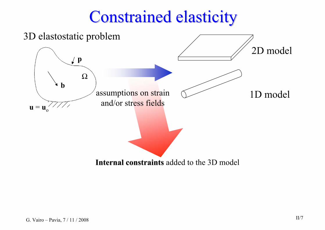
Internal constraintsInternal constraints added to the 3D model
b
p
u = uo
Ω
3D elastostatic problem2D model
1D model
Constrained elasticityConstrained elasticity
assumptions on strain and/or stress fields
G. Vairo – Pavia, 7 / 11 / 2008 II/7

Internal constraintsInternal constraints added to the 3D model
Lagrangian multipliersLagrangian multipliers can be employed to formulate the 3D constrained problem:
they give reactive constraintsreactive constraints belonging to dual spaces of those where constrained variables live
b
p
u = uo
3D elastostatic problem2D model
1D model
Constrained elasticityConstrained elasticity
assumptions on strain and/or stress fields
Ω
G. Vairo – Pavia, 7 / 11 / 2008 II/7

Constrained elasticityConstrained elasticity
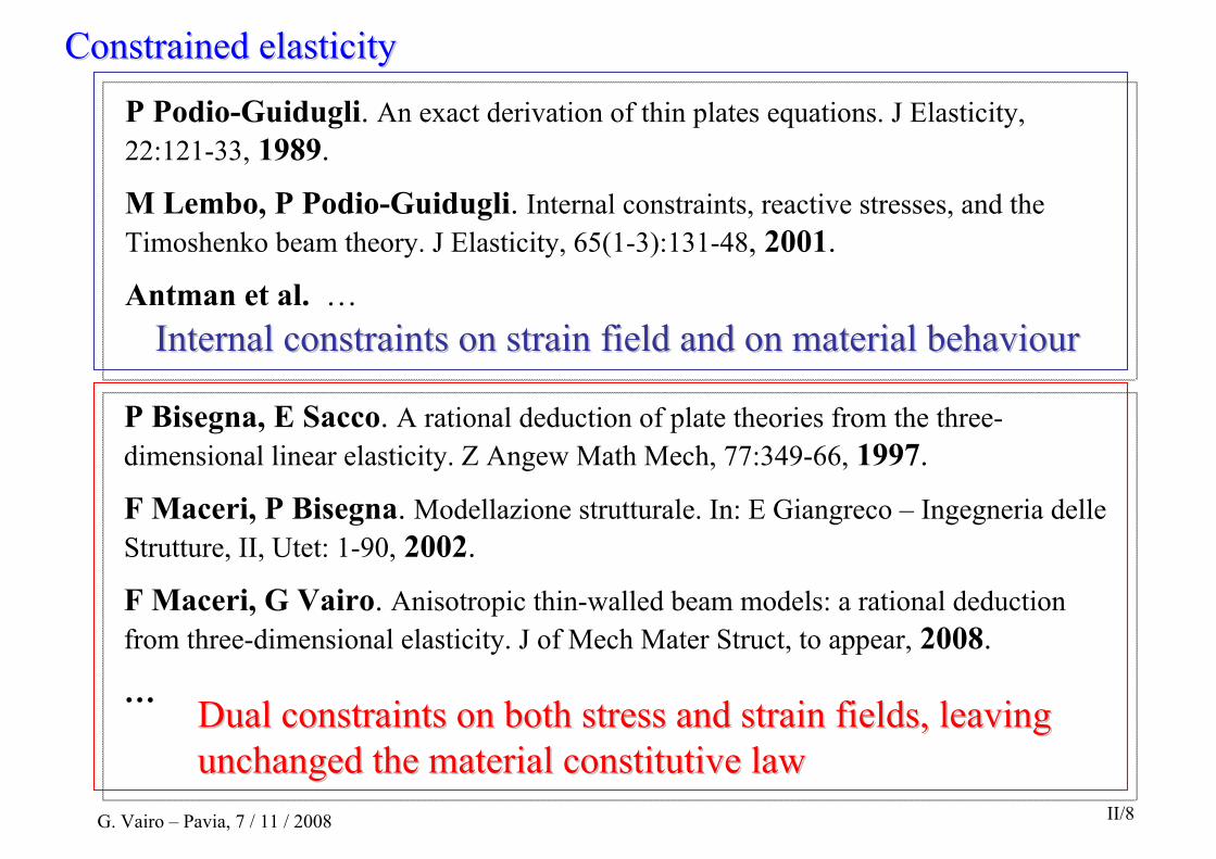
P Podio-Guidugli. An exact derivation of thin plates equations. J Elasticity, 22:121-33, 1989.
M Lembo, P Podio-Guidugli. Internal constraints, reactive stresses, and the Timoshenko beam theory. J Elasticity, 65(1-3):131-48, 2001.
Antman et al. …Internal constraints on strain field and on material behaviourInternal constraints on strain field and on material behaviour
G. Vairo – Pavia, 7 / 11 / 2008 II/8
P Podio-Guidugli. An exact derivation of thin plates equations. J Elasticity, 22:121-33, 1989.
M Lembo, P Podio-Guidugli. Internal constraints, reactive stresses, and the Timoshenko beam theory. J Elasticity, 65(1-3):131-48, 2001.
Antman et al. …Internal constraints on strain field and on material behaviourInternal constraints on strain field and on material behaviour
P Bisegna, E Sacco. A rational deduction of plate theories from the three-dimensional linear elasticity. Z Angew Math Mech, 77:349-66, 1997.
F Maceri, P Bisegna. Modellazione strutturale. In: E Giangreco – Ingegneria delle Strutture, II, Utet: 1-90, 2002.
F Maceri, G Vairo. Anisotropic thin-walled beam models: a rational deduction from three-dimensional elasticity. J of Mech Mater Struct, to appear, 2008.
…Dual constraints on both stress and strain fields, leaving Dual constraints on both stress and strain fields, leaving unchanged the material constitutive lawunchanged the material constitutive law
Constrained elasticityConstrained elasticity
G. Vairo – Pavia, 7 / 11 / 2008 II/8

b
p
u = uo
Dual constraints approachDual constraints approach
∫∫∫
∫∫
Ω∂∂
Ω∂Ω
ΩΩ
−⋅−⋅−⋅−
−∇⋅−⋅=
uf
dadadv
dvdv
o )(
)ˆ(21),,(
uuσnupub
εuσεεεσu CW
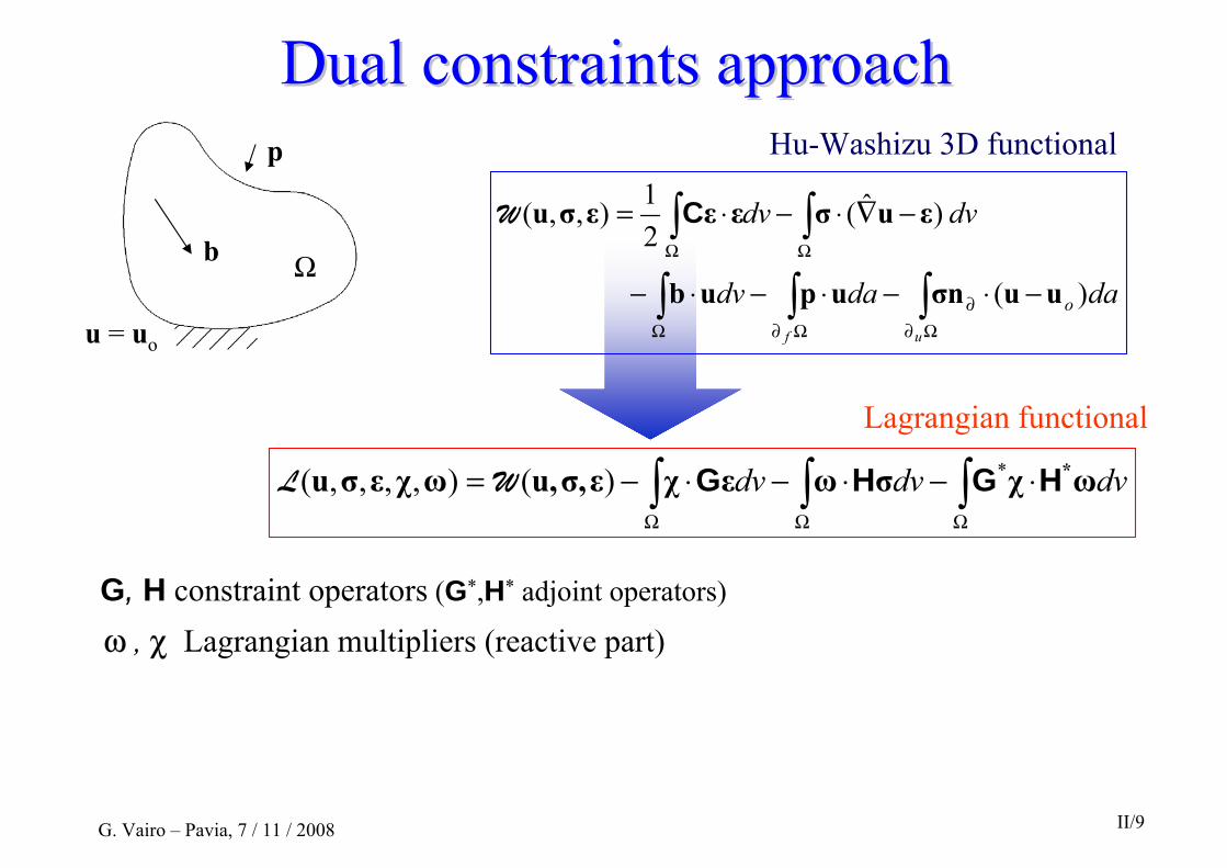
Hu-Washizu 3D functional
Ω
G. Vairo – Pavia, 7 / 11 / 2008 II/9
b
p
u = uo
Dual constraints approachDual constraints approach
∫∫∫ΩΩΩ
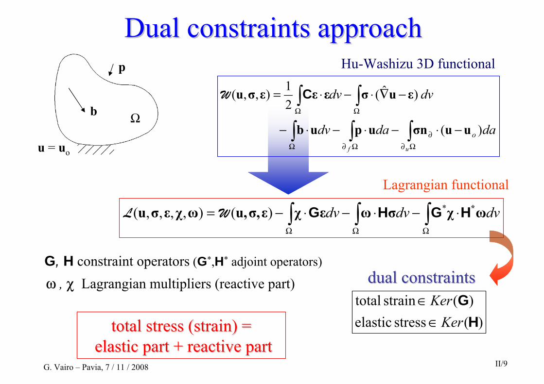
⋅−⋅−⋅−= dvdvdv ωχσωεχεσ,u,ωχεσu *HGHG *)(),,,,( WL
G, H constraint operators (G*,H* adjoint operators)
ω , χ Lagrangian multipliers (reactive part)
Hu-Washizu 3D functional
Lagrangian functional
∫∫∫
∫∫
Ω∂∂
Ω∂Ω
ΩΩ
−⋅−⋅−⋅−
−∇⋅−⋅=
uf
dadadv
dvdv
o )(
)ˆ(21),,(
uuσnupub
εuσεεεσu CW
Ω
G. Vairo – Pavia, 7 / 11 / 2008 II/9
b
p
u = uo
Dual constraints approachDual constraints approach
total stress (strain) = total stress (strain) = elastic part + reactive partelastic part + reactive part
dual constraintsdual constraints
)(stress elastic)(strain totalH
GKer
Ker∈
∈
G, H constraint operators (G*,H* adjoint operators)
ω , χ Lagrangian multipliers (reactive part)
Hu-Washizu 3D functional
Lagrangian functional
Ω∫∫∫
∫∫
Ω∂∂
Ω∂Ω
ΩΩ
−⋅−⋅−⋅−
−∇⋅−⋅=
uf
dadadv
dvdv
o )(
)ˆ(21),,(
uuσnupub
εuσεεεσu CW
∫∫∫ΩΩΩ
⋅−⋅−⋅−= dvdvdv ωχσωεχεσ,u,ωχεσu *HGHG *)(),,,,( WL
G. Vairo – Pavia, 7 / 11 / 2008 II/9
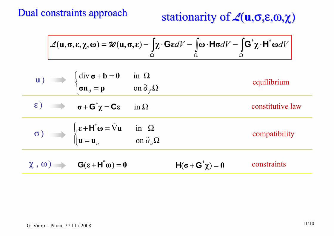
⎩⎨⎧
Ω∂=Ω=+
∂ fon in div
pσn0bσ
Dual constraints approachDual constraints approach stationarity of stationarity of LL((uu,,σσ,,εε,,ωω,,χχ))
u )
Ω=+ in * εχσ CG
on in ˆ*
⎪⎩
⎪⎨⎧
Ω∂=Ω∇=+
uouuuωε H
ε )
σ )
0χσ =+ )( *GH0ωε =+ )( *HG
equilibrium
constitutive law
compatibility
constraintsχ , ω )
∫∫∫ΩΩΩ
⋅−⋅−⋅−= dVdVdV ωχσωεχεσ,u,ωχεσu *HGHG *)(),,,,( WL
G. Vairo – Pavia, 7 / 11 / 2008 II/10

⎩⎨⎧
Ω∂=Ω=+
∂ fon in div
pσn0bσ
Dual constraints approachDual constraints approach stationarity of stationarity of LL((uu,,σσ,,εε,,ωω,,χχ))
u )
Ω=+ in * εχσ CG
on in ˆ*
⎪⎩
⎪⎨⎧
Ω∂=Ω∇=+
uouuuωε H
ε )
σ )
0χσ =+ )( *GH0ωε =+ )( *HG
equilibrium
constitutive law
compatibility
constraintsχ , ω )
total stress
total strainelastic stress
elastic strainχσ *G+ ωε *H+
∫∫∫ΩΩΩ
⋅−⋅−⋅−= dVdVdV ωχσωεχεσ,u,ωχεσu *HGHG *)(),,,,( WL
G. Vairo – Pavia, 7 / 11 / 2008 II/10

stationary conditions of the Lagrangian functional L(u,σ,ε,ω,χ) with respect to elastic strain ε and total stress σ allow to eliminate ε and σ themselves and to obtain the energy-type functional
Dual constraints approachDual constraints approach
∫∫∫∫Ω∂ΩΩΩ
⋅−⋅−∇⋅−−∇⋅−∇=f
dadvdvdv upubuχωuωuωχu ˆ)ˆ()ˆ(21),,( ** GHHCE
ωε
ωuε
uε
*
* )ˆ(
ˆ
HH
=
−∇=
∇=
react
el
tot
χσ
ωuσ
χωuσ
*react
el
*tot
GHC
GHC
−=
−∇=
−−∇=
)ˆ(
)ˆ(*
*
defined on the manifold Ω∂= uo on uu
G. Vairo – Pavia, 7 / 11 / 2008 II/11

Dual constraints approachDual constraints approach
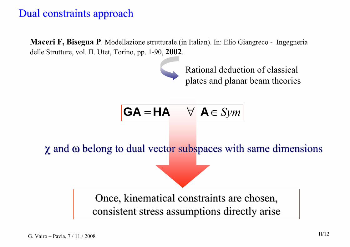
Maceri F, Bisegna P. Modellazione strutturale (in Italian). In: Elio Giangreco - Ingegneria delle Strutture, vol. II. Utet, Torino, pp. 1-90, 2002.
Sym ∈∀= A HA GA
Rational deduction of classical plates and planar beam theories
G. Vairo – Pavia, 7 / 11 / 2008 II/12
Dual constraints approachDual constraints approach
Maceri F, Bisegna P. Modellazione strutturale (in Italian). In: Elio Giangreco - Ingegneria delle Strutture, vol. II. Utet, Torino, pp. 1-90, 2002.
Sym ∈∀= A HA GA
χ χ and and ωω belong to dual vector subspaces with same dimensionsbelong to dual vector subspaces with same dimensions
Once, kinematical constraints are chosen, Once, kinematical constraints are chosen, consistent stress assumptions directly ariseconsistent stress assumptions directly arise
Rational deduction of classical plates and planar beam theories
G. Vairo – Pavia, 7 / 11 / 2008 II/12
x (i)
y (j)
O
P
so
n (η)t
s S
x~sl
C
xcr
p
tn
kx
y
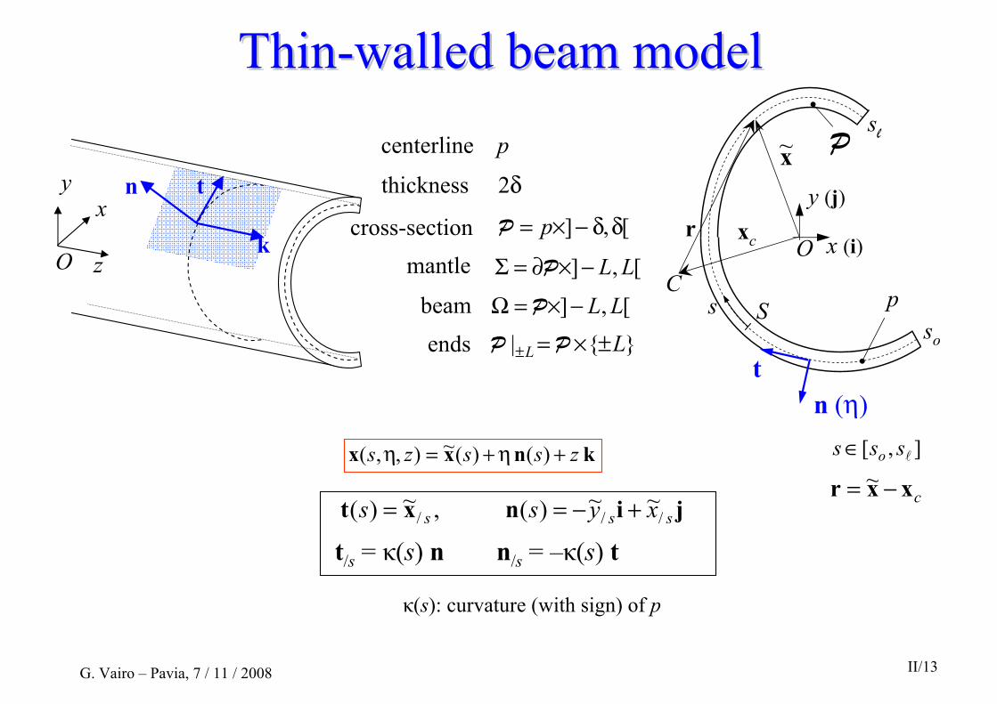
O zcross-section
}{| LL ±×=± PPends[,] LL−×=Ω P
[,] LL−×∂=Σ P
[,] δδ−×= pP
beam
mantle
centerline p
thickness 2δ
ThinThin--walled beam modelwalled beam model
κ(s): curvature (with sign) of p
jinxt sss xyss ///~~)( ,~)( +−==
t/s = κ(s) n n/s = –κ(s) t
knxx )( )(~),,( zsszs +η+=η ],[ lsss o∈
cxxr −= ~
G. Vairo – Pavia, 7 / 11 / 2008 II/13

ThinThin--walled beam modelwalled beam model
x (i)
y (j)
O
P
so
n (η)t
s S
x~sl
C
xcr
p
∫ ∫∫δ
δ−
=p
dsdηηsjda ),( (.) (.)P
∫δ
δ−δ= dηηsjzηsfzsf ),( ),,(
21),(
average over the thickness domain
]1[)( ηκ(s)s,ηj −=
knt // ffj
ff s ′++=∇ η zff
∂∂=′
G. Vairo – Pavia, 7 / 11 / 2008 II/14
ThinThin--walled beam modelwalled beam model
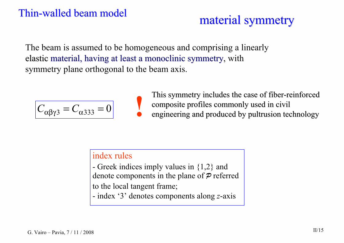
The beam is assumed to be homogeneous and comprising a linearly elastic elastic material, having at least a monoclinic symmetrymaterial, having at least a monoclinic symmetry, with symmetry plane orthogonal to the beam axis.
03333 == ααβγ CC
index rules- Greek indices imply values in {1,2} and denote components in the plane of P referred to the local tangent frame;- index ‘3’ denotes components along z-axis
This symmetry includes the case of fiberThis symmetry includes the case of fiber--reinforced reinforced composite profiles commonly used in civil composite profiles commonly used in civil engineering and produced by pultrusion technologyengineering and produced by pultrusion technology!
material symmetrymaterial symmetry
G. Vairo – Pavia, 7 / 11 / 2008 II/15

NoNo--shear beam modelshear beam model
strain and stress dual constraintsstrain and stress dual constraints
Vlasov / Euler-Bernoulli
G. Vairo – Pavia, 7 / 11 / 2008 II/16
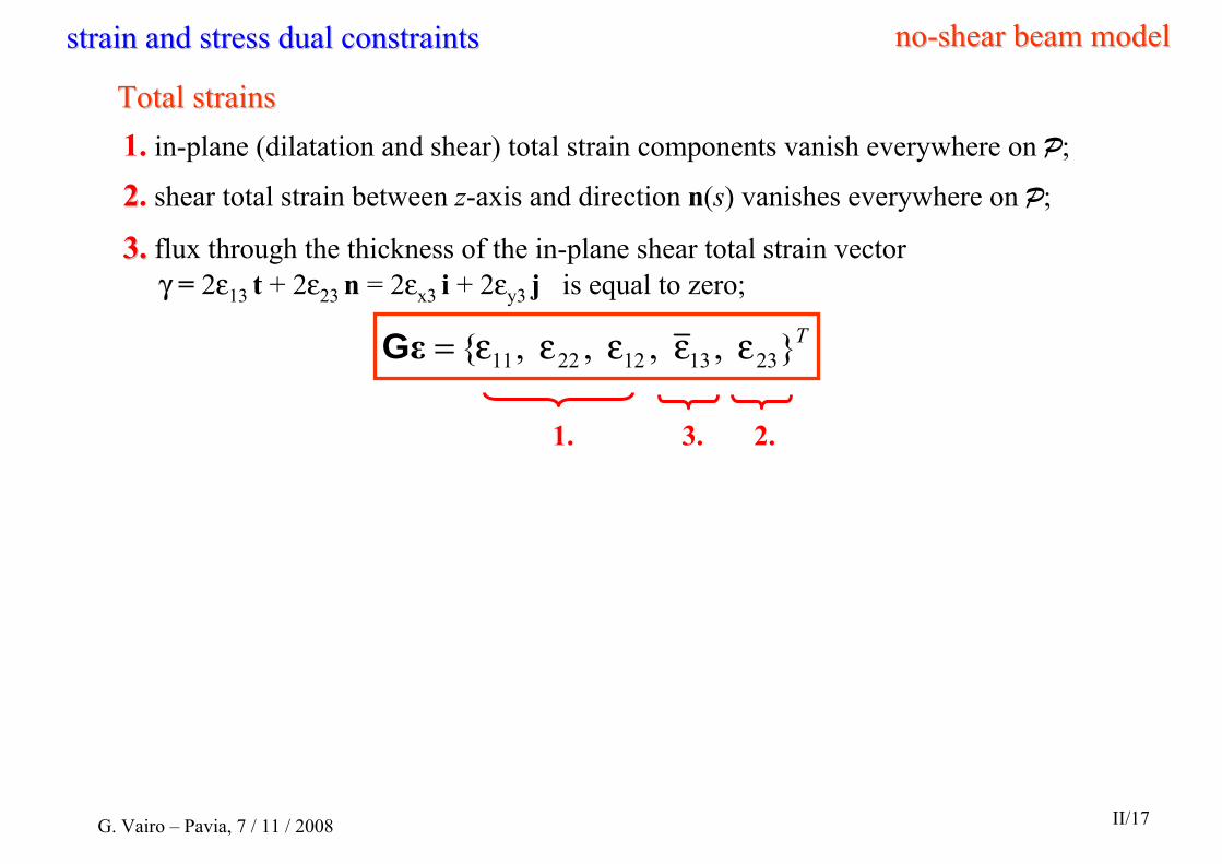
1. 3. 2.
1. in-plane (dilatation and shear) total strain components vanish everywhere on P;
22. shear total strain between z-axis and direction n(s) vanishes everywhere on P;
3.3. flux through the thickness of the in-plane shear total strain vector γ = 2ε13 t + 2ε23 n = 2εx3 i + 2εy3 j is equal to zero;
Total strainsTotal strains
T} , , , ,{ 2313122211 εεεεε=εG
nono--shear beam modelshear beam modelstrain and stress dual constraintsstrain and stress dual constraints
G. Vairo – Pavia, 7 / 11 / 2008 II/17

Total strainsTotal strains
T} , , , ,{ 2313122211 σσσσσ=σH
1. elastic stress vector on every plane parallel to the z-axis is parallel to k;
22. shear elastic stress between z-axis and direction n(s) vanishes everywhere on P;
3.3. flux through the thickness of the in-plane shear elastic stress vector τ = τ13 t + τ23 n = τx3 i + τy3 j is equal to zero;
Elastic stressesElastic stresses
),( ),,( 0 ,0 131313131313 zszseltot χ=χω=ω⇒=σ=εRemark:
1. in-plane (dilatation and shear) total strain components vanish everywhere on P;
22. shear total strain between z-axis and direction n(s) vanishes everywhere on P;
3.3. flux through the thickness of the in-plane shear total strain vector γ = 2ε13 t + 2ε23 n = 2εx3 i + 2εy3 j is equal to zero;
T} , , , ,{ 2313122211 εεεεε=εG
nono--shear beam modelshear beam modelstrain and stress dual constraintsstrain and stress dual constraints
G. Vairo – Pavia, 7 / 11 / 2008II/17
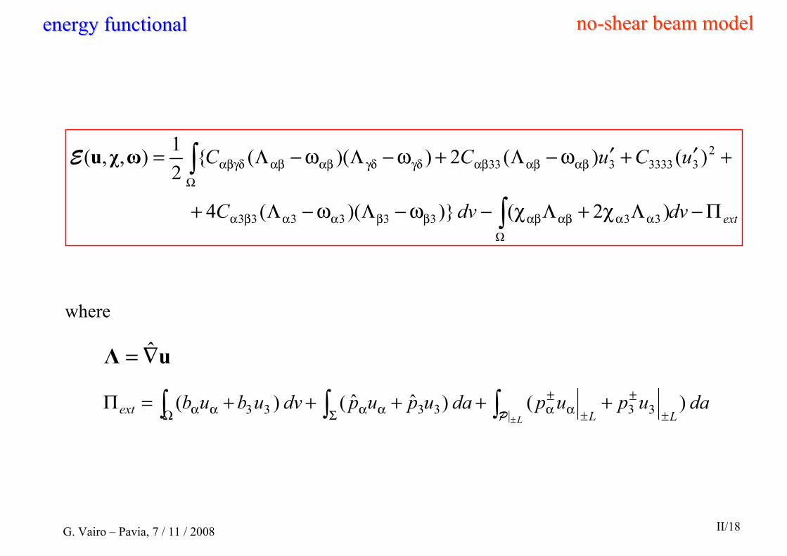
extdvdvC
uCuCC
Π−Λχ+Λχ−ω−Λω−Λ+
+′+′ω−Λ+ω−Λω−Λ=
∫
∫
Ωαααβαβββααβα
Ωαβαβαβγδγδαβαβαβγδ
)2( )})((4
)()(2))(({21),,(
33333333
233333333ωχuE
∫∫∫± ±
±±α
±αΣ ααΩ αα +++++=Π
Ldaupupdaupupdvubub
LLext | 33 3333 )( )ˆˆ( )(P
uΛ ∇= ˆ
where
nono--shear beam modelshear beam modelenergy functionalenergy functional
G. Vairo – Pavia, 7 / 11 / 2008 II/18

stationarity of stationarity of EE((uu,,ωω,,χχ) with respect to ) with respect to χχ gives the equationsgives the equations
nono--shear beam modelshear beam modeldisplacement fielddisplacement field
G. Vairo – Pavia, 7 / 11 / 2008 II/19
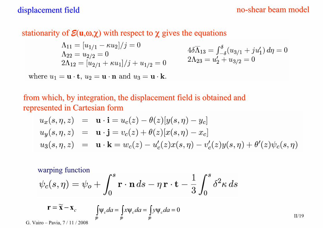
cxxr −= ~0=ψ=ψ=ψ ∫∫∫ daydaxda ccc
PPP
from which, by integration, the displacement field is obtained afrom which, by integration, the displacement field is obtained and nd represented in Cartesian formrepresented in Cartesian form
warping function
nono--shear beam modelshear beam modeldisplacement fielddisplacement field
stationarity of stationarity of EE((uu,,ωω,,χχ) with respect to ) with respect to χχ gives the equationsgives the equations
G. Vairo – Pavia, 7 / 11 / 2008II/19
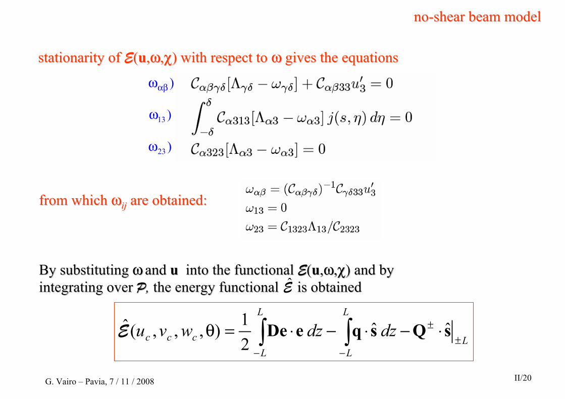
)αβω
)13ω
)23ω
nono--shear beam modelshear beam model
stationarity of stationarity of EE((uu,,ωω,,χχ) with respect to ) with respect to ωω gives the equationsgives the equations
from which from which ωωijij are obtained:are obtained:
By substituting By substituting ωω and and uu into the functional into the functional EE((uu,,ωω,,χχ) and by ) and by integrating over integrating over PP, , the energy functional is obtainedthe energy functional is obtainedE
L
L
L
L
Lccc dzdzwvu
±±
−−
⋅−⋅−⋅=θ ∫∫ sQsqeDe ˆ ˆ 21),,,(E
G. Vairo – Pavia, 7 / 11 / 2008 II/20

nono--shear beam modelshear beam modelpure potential energy functionalpure potential energy functional
L
L
L
L
Lccc dzdzwvu
±±
−−
⋅−⋅−⋅=θ ∫∫ sQsqeDe ˆ ˆ 21),,,(E
forcesdend-locatedgeneralizeforcesddistributedgeneralizestrainstotaldgeneralizentsdisplacemedgeneralize
: : : :ˆ
±Qqes
D: generalized elasticity matrix of the beam
Tzyxzyx
Tzyxzyx
MMMMQQQ
mmmmqqq
},,,,,,{
},,,,,,{±ψ
±±±±±±±
ψ
=
=
Q
qT
ccc
Tccccc
uvw
uvwvu
},,,,{
},,,,,,{ˆ
θ′θ ′′′′′′−′=
θ′θ′′−=
e
s
G. Vairo – Pavia, 7 / 11 / 2008 II/21

nono--shear beam modelshear beam modelpure potential energy functionalpure potential energy functional
L
L
L
L
Lccc dzdzwvu
±±
−−
⋅−⋅−⋅=θ ∫∫ sQsqeDe ˆ ˆ 21),,,(E
Reduced elastic moduliReduced elastic moduli
reduced constitutive law comes out from the procedure adopted and is not a-priori enforced by a constrained constitutive law
G. Vairo – Pavia, 7 / 11 / 2008 II/22

nono--shear beam modelshear beam modelpure potential energy functionalpure potential energy functional
O: centroid for Ω, C: twinsting center for P, x and y principal for P, S: sectorial centroid for p D: diagonal
G. Vairo – Pavia, 7 / 11 / 2008 II/23
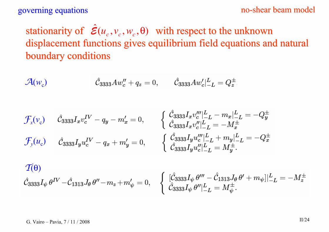
stationarity of with respect to the ustationarity of with respect to the unknown nknown displacement functions gives equilibrium field equations and natdisplacement functions gives equilibrium field equations and naturaluralboundary conditionsboundary conditions
nono--shear beam modelshear beam modelgoverning equationsgoverning equations
),,,(ˆ θccc wvuE
A(wc)
Fx(vc)
Fy(uc)
T(θ)
G. Vairo – Pavia, 7 / 11 / 2008 II/24
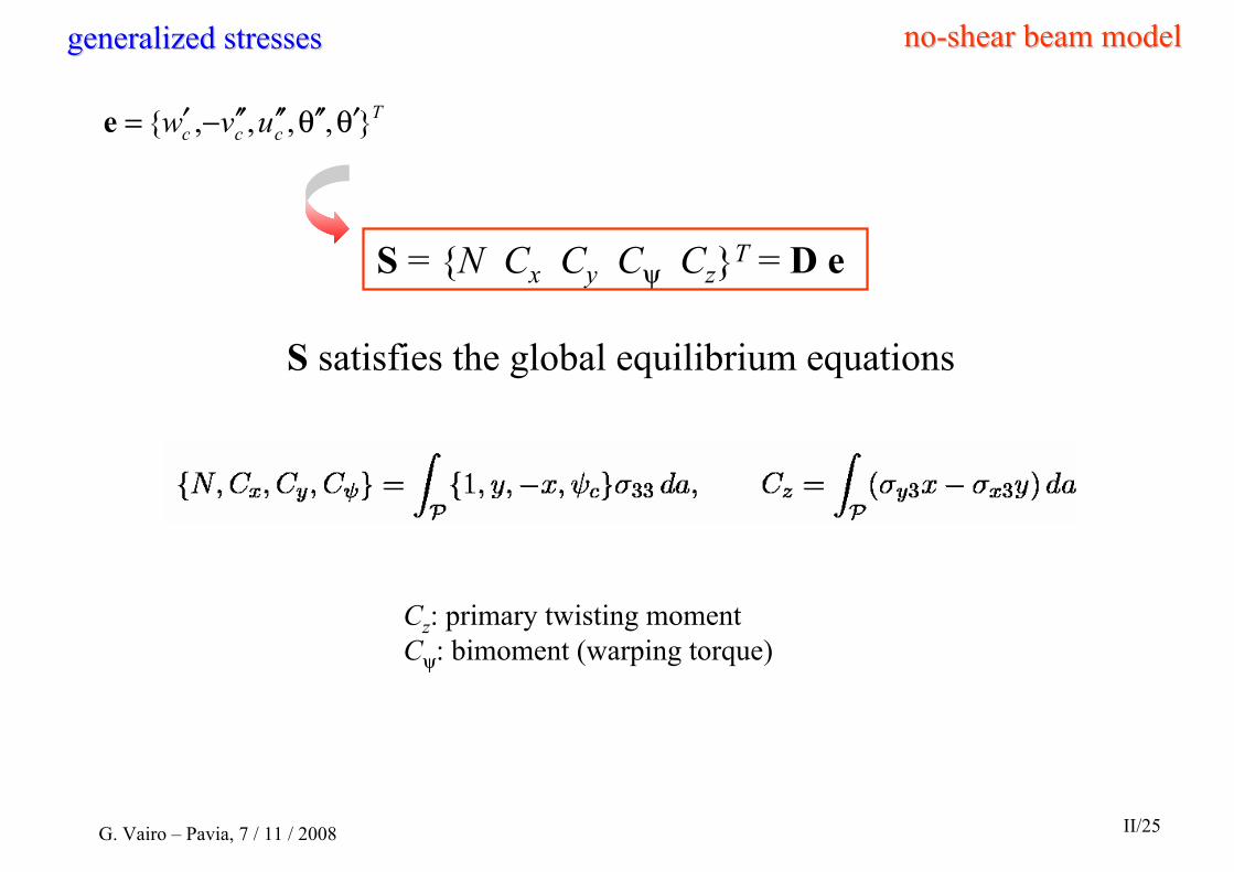
S = {N Cx Cy Cψ Cz}T = D e
S satisfies the global equilibrium equations
Cz: primary twisting momentCψ: bimoment (warping torque)
nono--shear beam modelshear beam modelgeneralized stressesgeneralized stresses
Tccc uvw },,,,{ θ′θ ′′′′′′−′=e
G. Vairo – Pavia, 7 / 11 / 2008 II/25
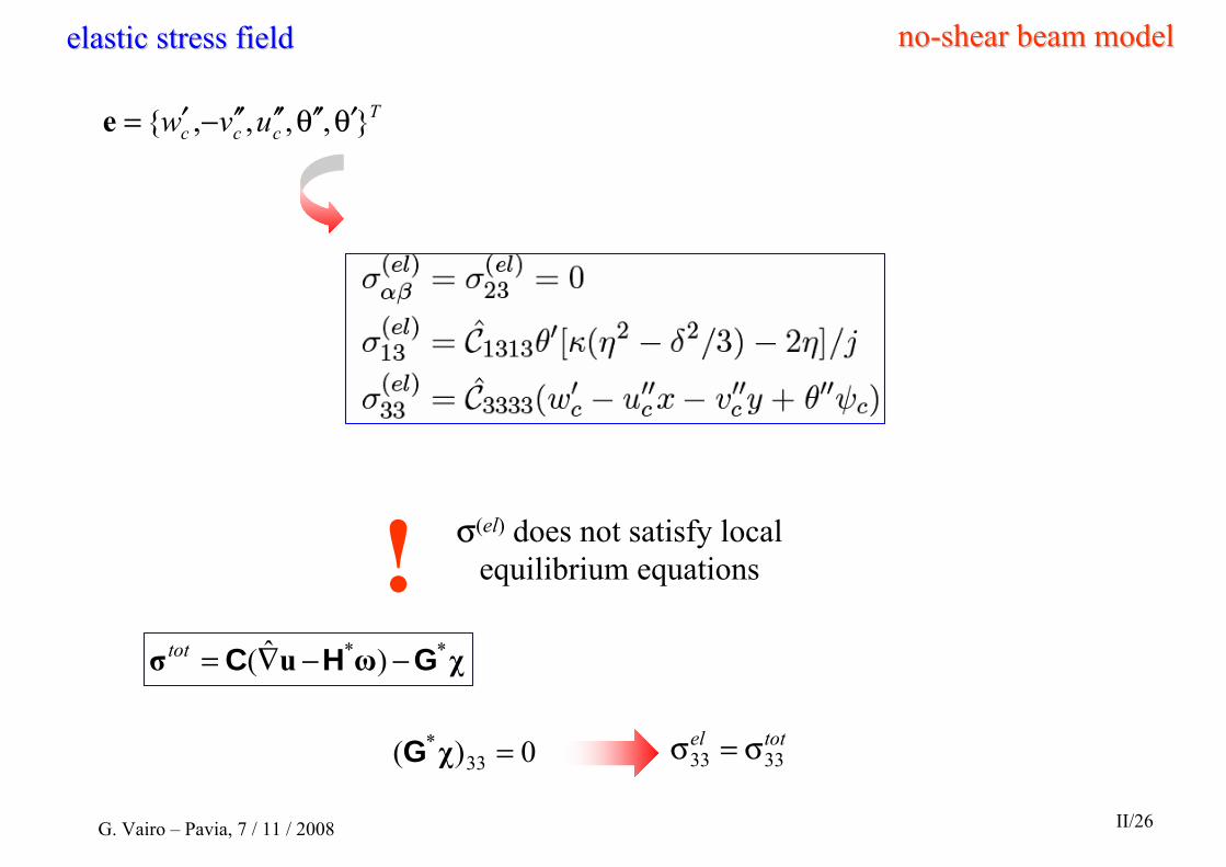
σ(el) does not satisfy local equilibrium equations!
χωuσ *tot GHC −−∇= )ˆ( *
totel3333 σ=σ0)( 33 =χ*G
nono--shear beam modelshear beam modelelastic stress fieldelastic stress field
Tccc uvw },,,,{ θ′θ ′′′′′′−′=e
G. Vairo – Pavia, 7 / 11 / 2008 II/26

disregarding high-oder effects (related to curvature and thickness)
nono--shear beam modelshear beam model
also, isotropic material
Classical Vlasov theory
reduction to classical modelsreduction to classical models
G. Vairo – Pavia, 7 / 11 / 2008 II/27

CurvatureCurvature’’s influences influence
l
5.2ˆˆ
1313
3333 =CCHomogeneous beam, comprised by material with a constitutive
symmetry at least monoclinic and symmetry plane orthogonal to x3
l
m3M3
1/κ
δ
δκ δκ
lκ = 5lκ = 10lκ = 20lκ = 40
A A
θA(κ)/θA
θA(κ)/θA
G. Vairo – Pavia, 7 / 11 / 2008 II/28
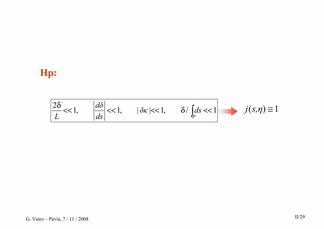
1)( ≅s,ηj1/ ,1|| ,1 ,12 <<δ<<<<<<δ∫pdsδκ
dsdδ
L
Hp:
G. Vairo – Pavia, 7 / 11 / 2008 II/29

FirstFirst--order shearorder shear--deformable beam modeldeformable beam model
strain and stress dual constraintsstrain and stress dual constraints
Vlasov / Timoshenko
G. Vairo – Pavia, 7 / 11 / 2008 II/30
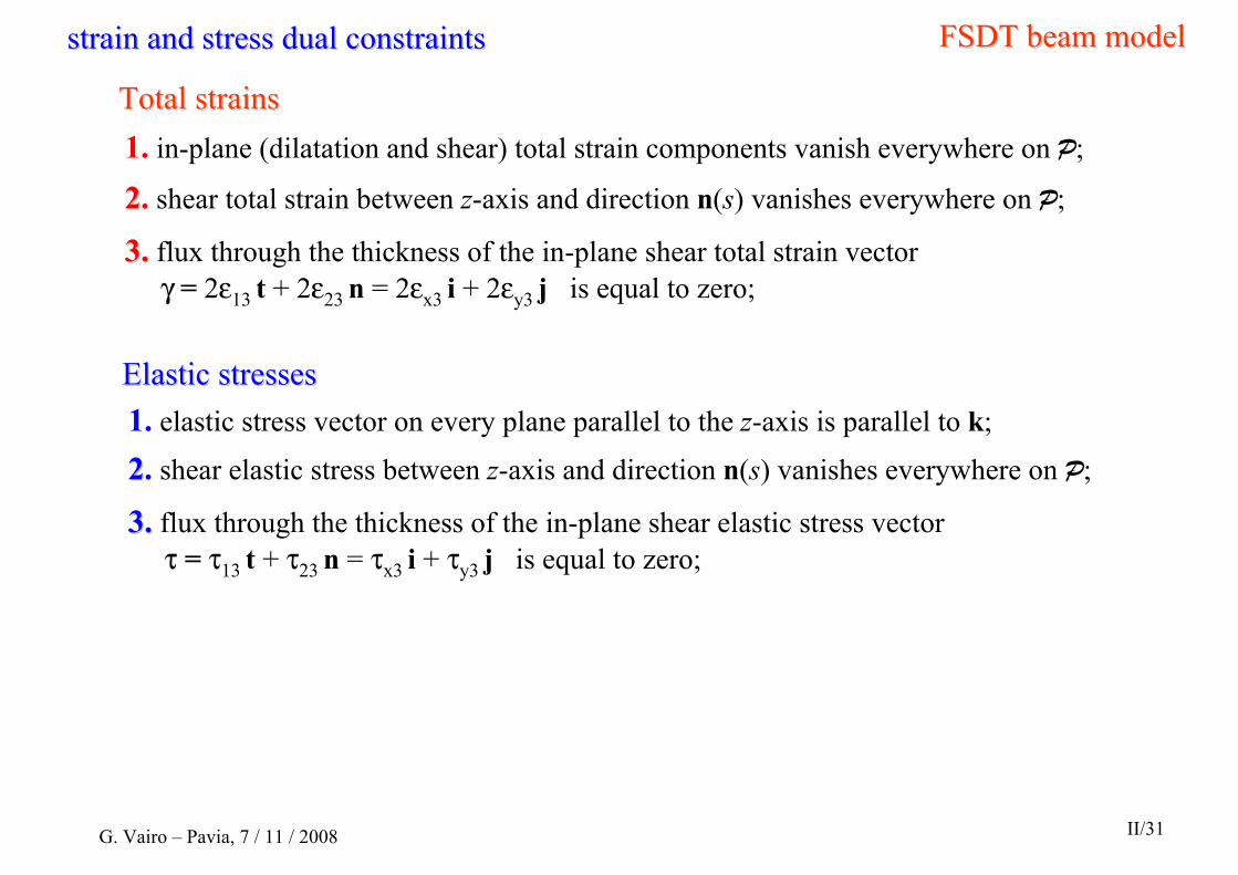
1. in-plane (dilatation and shear) total strain components vanish everywhere on P;
22. shear total strain between z-axis and direction n(s) vanishes everywhere on P;
3.3. flux through the thickness of the in-plane shear total strain vector γ = 2ε13 t + 2ε23 n = 2εx3 i + 2εy3 j is equal to zero;
Total strainsTotal strains
FSDT beam modelFSDT beam modelstrain and stress dual constraintsstrain and stress dual constraints
1. elastic stress vector on every plane parallel to the z-axis is parallel to k;
22. shear elastic stress between z-axis and direction n(s) vanishes everywhere on P;
3.3. flux through the thickness of the in-plane shear elastic stress vector τ = τ13 t + τ23 n = τx3 i + τy3 j is equal to zero;
Elastic stressesElastic stresses
G. Vairo – Pavia, 7 / 11 / 2008 II/31

1. in-plane (dilatation and shear) total strain components vanish everywhere on P;
22’’. shear total strain between z-axis and direction n(s) vanishes everywhere on P;
33’’.. flux through the thickness of the in-plane shear total strain vector γ = 2ε13 t + 2ε23 n = 2εx3 i + 2εy3 j is equal to zero;
Total strainsTotal strains
FSDT beam modelFSDT beam modelstrain and stress dual constraintsstrain and stress dual constraints
is constant over
is constant over PP
1. elastic stress vector on every plane parallel to the z-axis is parallel to k;
22’’. shear elastic stress between z-axis and direction n(s) vanishes everywhere on P;
33’’.. flux through the thickness of the in-plane shear elastic stress vector τ = τ13 t + τ23 n = τx3 i + τy3 j is equal to zero;
Elastic stressesElastic stresses
is constant over
is constant over PP
T} , ,)(2 , , ,{ 2/231/231/13122211 σσσδσσσ=σH
T} , ,)(2 , , ,{ 2/231/231/13122211 εεεδεεε=εG
G. Vairo – Pavia, 7 / 11 / 2008 II/31
FSDT beam modelFSDT beam model
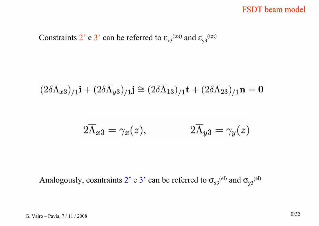
Analogously, cosntraints 2’ e 3’ can be referred to σx3(el) and σy3
(el)
Constraints 2’ e 3’ can be referred to εx3(tot) and εy3
(tot)
G. Vairo – Pavia, 7 / 11 / 2008 II/32

∫∫∫± ±
±±α
±αΣ ααΩ αα +++++=Π
Ldaupupdaupupdvubub
LLext | 33 3333 )( )ˆˆ( )(P
uΛ ∇= ˆ
where
energy functionalenergy functional FSDT beam modelFSDT beam model
G. Vairo – Pavia, 7 / 11 / 2008 II/33
FirstFirst--order shearorder shear--deformable beam modeldeformable beam modelaccounting for warping shear effectsaccounting for warping shear effects
strain and stress dual constraintsstrain and stress dual constraints
G. Vairo – Pavia, 7 / 11 / 2008 II/34
1. 3. 2.
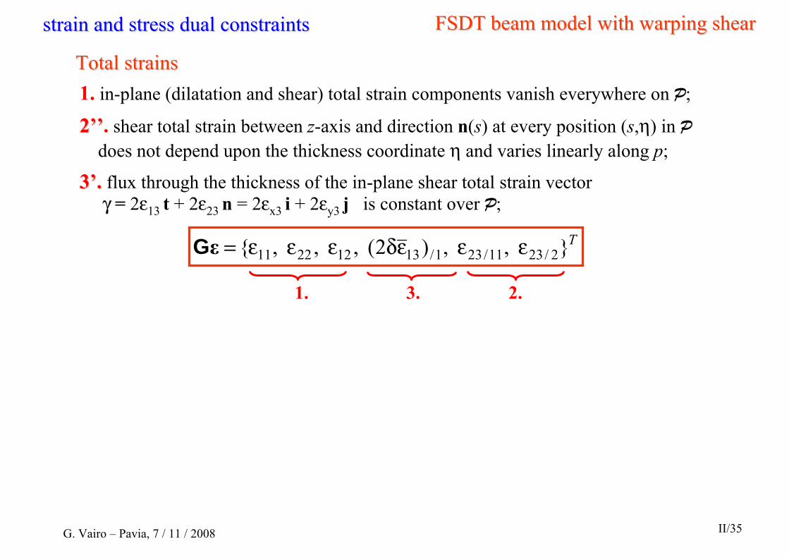
1. in-plane (dilatation and shear) total strain components vanish everywhere on P;
22’’’’. shear total strain between z-axis and direction n(s) at every position (s,η) in Pdoes not depend upon the thickness coordinate η and varies linearly along p;
33’’.. flux through the thickness of the in-plane shear total strain vector γ = 2ε13 t + 2ε23 n = 2εx3 i + 2εy3 j is constant over P;
Total strainsTotal strains
T} , ,)2( , , ,{ 2/2311/231/13122211 εεεδεεε=εG
FSDT beam model with warping shearFSDT beam model with warping shearstrain and stress dual constraintsstrain and stress dual constraints
G. Vairo – Pavia, 7 / 11 / 2008 II/35

1. in-plane (dilatation and shear) total strain components vanish everywhere on P;
22’’’’. shear total strain between z-axis and direction n(s) at every position (s,η) in Pdoes not depend upon the thickness coordinate η and varies linearly along p;
33’’.. flux through the thickness of the in-plane shear total strain vector γ = 2ε13 t + 2ε23 n = 2εx3 i + 2εy3 j is constant over P;
Total strainsTotal strains
T} , ,)2( , , ,{ 2/2311/231/13122211 εεεδεεε=εG
T} , ,)2( , , ,{ 2/2311/231/13122211 σσσδσσσ=σH
1. elastic stress vector on every plane parallel to the z-axis is parallel to k;
22’’’’. shear elastic stress between z-axis and direction n(s) at every position (s,η) in does not depend upon the thickness coordinate η and varies linearly along p;
33’’.. flux through the thickness of the in-plane shear elastic stress vector τ = τ13 t + τ23 n = τx3 i + τy3 j is constant over ;
Elastic stressesElastic stresses
P
P
FSDT beam model with warping shearFSDT beam model with warping shearstrain and stress dual constraintsstrain and stress dual constraints
G. Vairo – Pavia, 7 / 11 / 2008 II/35
extdv
dvCC
CuC
uCC
Π−Λχ+Λχ+Λδχ+Λχ−
+ω+ω−Λ+δω+Λ+
+ω+ω−Λδω+Λ+′+
+′ω−Λ+ω−Λω−Λ=
∫
∫
Ωαβαβ
Ωαβαβαβγδγδαβαβαβγδ
)]~~(2)2(2[
}]~~[4])2([4
]~~][)2([8)(
)(2))(({21),,(
2/232311/23131/1313
22/2311/13232323
21/13131313
2/2311/13231/131313232
33333
333ωχuE
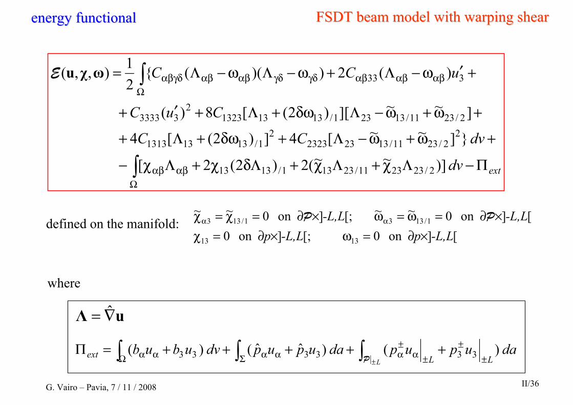
defined on the manifold:[]on 0 [;]on 0
[]on 0~~ [;]on 0~~
1313
1/1331/133
-L,Lp-L,Lp-L,L-L,L
×∂=ω×∂=χ×∂=ω=ω×∂=χ=χ αα PP
∫∫∫± ±
±±α
±αΣ ααΩ αα +++++=Π
Ldaupupdaupupdvubub
LLext | 33 3333 )( )ˆˆ( )(P
uΛ ∇= ˆ
where
FSDT beam model with warping shearFSDT beam model with warping shearenergy functionalenergy functional
G. Vairo – Pavia, 7 / 11 / 2008 II/36

0 0
0
2/111/2
2/2
21/1
=+κ+=
=κ−
uuuu
uu
stationarity of stationarity of EE((uu,,ωω,,χχ) with respect to ) with respect to χχ gives the equationsgives the equations
00
0 ] [
22/32/2
211/311/2
1/111/3
=+′=+′
=′+∫δ
δ−
uuuu
dnuu
displacement fielddisplacement field FSDT beam model with warping shearFSDT beam model with warping shear
G. Vairo – Pavia, 7 / 11 / 2008 II/37
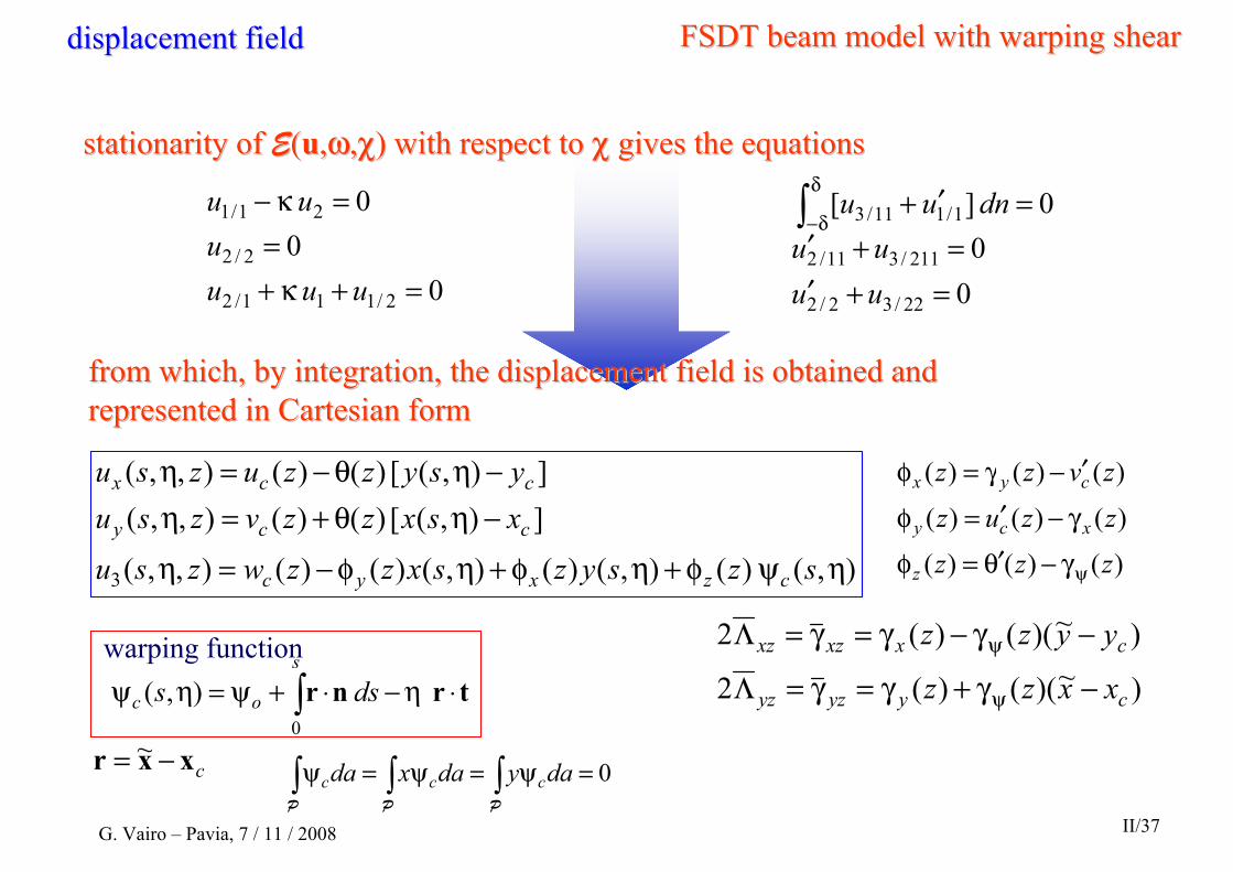
from which, by integration, the displacement field is obtained afrom which, by integration, the displacement field is obtained and nd represented in Cartesian formrepresented in Cartesian form
),(0
trnr ⋅η−⋅+ψ=ηψ ∫s
oc dsswarping function
0 0
0
2/111/2
2/2
21/1
=+κ+=
=κ−
uuuu
uu
stationarity of stationarity of EE((uu,,ωω,,χχ) with respect to ) with respect to χχ gives the equationsgives the equations
00
0 ] [
22/32/2
211/311/2
1/111/3
=+′=+′
=′+∫δ
δ−
uuuu
dnuu
),( )(),()(),()()(),,(
]),([ )()(),,(]),([ )()(),,(
3 ηψφ+ηφ+ηφ−=η
−ηθ+=η−ηθ−=η
szsyzsxzzwzsu
xsxzzvzsuysyzzuzsu
czxyc
ccy
ccx
cxxr −= ~
)()()(
)()()(
)()()(
zzz
zzuz
zvzz
z
xcy
cyx
ψγ−θ′=φ
γ−′=φ
′−γ=φ
)~)(()(2
)~)(()(2
cyyzyz
cxxzxz
xxzz
yyzz
−γ+γ=γ=Λ
−γ−γ=γ=Λ
ψ
ψ
0=ψ=ψ=ψ ∫∫∫ daydaxda cccPPP
displacement fielddisplacement field FSDT beam model with warping shearFSDT beam model with warping shear
G. Vairo – Pavia, 7 / 11 / 2008 II/37

{ }{ } 0 ]~~[])2([
0 ]~~[])2([
0 ]~~[])2([
0][
2/2/2311/132323231/13131323
11/2/2311/132323231/13131323
1/2/2311/132313231/13131313
333
=ω+ω−Λ+δω+Λ=ω+ω−Λ+δω+Λ
=⎭⎬⎫
⎩⎨⎧ ηω+ω−Λ+δω+Λ
=′+ω−Λ
∫δ
δ−
ββγδγδαβγδ
CCCC
dCC
uCC)αβω
)13ω
)~13ω
)~23ω
from which from which ωωijij are obtained.are obtained.
By substituting By substituting ωω and and uu into the functional into the functional EE((uu,,ωω,,χχ) and by ) and by integrating over integrating over PP, , the energy functional is obtainedthe energy functional is obtained
L
L
L
L
Lzyxccc dzdzwvu ±
±
−−
⋅−⋅−⋅=θφφφ ∫∫ sQsqeDe ˆ ˆ 21),,,,,,(E
stationarity of stationarity of EE((uu,,ωω,,χχ) with respect to ) with respect to ωω gives the equationsgives the equations
E
reactive strainsreactive strains FSDT beam model with warping shearFSDT beam model with warping shear
G. Vairo – Pavia, 7 / 11 / 2008 II/38
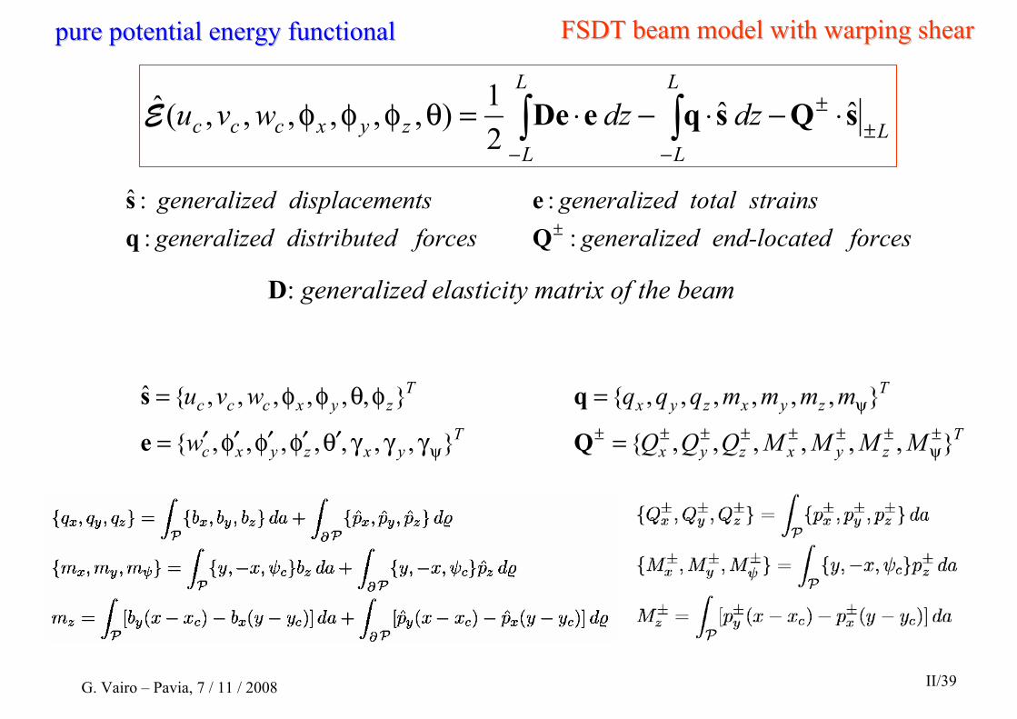
forcesdend-locatedgeneralizeforcesddistributedgeneralizestrainstotaldgeneralizentsdisplacemedgeneralize
: : : :ˆ
±Qqes
D: generalized elasticity matrix of the beam
L
L
L
L
Lzyxccc dzdzwvu ±
±
−−
⋅−⋅−⋅=θφφφ ∫∫ sQsqeDe ˆ ˆ 21),,,,,,(E
Tzyxzyx
Tzyxzyx
MMMMQQQ
mmmmqqq
},,,,,,{
},,,,,,{±ψ
±±±±±±±
ψ
=
=
Q
qT
yxzyxc
Tzyxccc
w
wvu
},,,,,,,{
},,,,,,{ˆ
ψγγγθ′φ′φ′φ′′=
φθφφ=
e
s
pure potential energy functionalpure potential energy functional FSDT beam model with warping shearFSDT beam model with warping shear
G. Vairo – Pavia, 7 / 11 / 2008 II/39
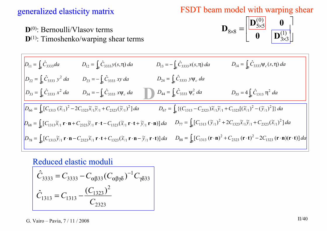
daCD ∫=P 333311
ˆ dasyCD ∫ η=P
),(ˆ333312 dasxCD ∫ η−=
P ),(ˆ
333313 dasCD c∫ ηψ=P
),(ˆ333314
dayCD ∫=P
ˆ 2333322 daxyCD ∫−=
P ˆ
333323 dayCD c∫ ψ=P
ˆ333324
daxCD ∫=P
ˆ 2333333 daxCD c∫ ψ−=
P ˆ
333334 daCD c∫ ψ=P
ˆ 2333344 daCD ∫ η=
P ˆ4 2
131355
dayCyxCxCD ∫ +−=P
])~(~~2)~( [ 21/23231/1/1323
21/131366 dayxCyxCCD ∫ −+−=
P ]})~()~([~~){( 2
1/2
1/13231/1/2323131367
dayxCyCxCD ∫ ⋅+⋅−⋅+⋅=P
)] ~ ~( ~ ~[ 1/1/13231/23231/131368 nrtrtrnr daxCyxCyCD ∫ ++=P
])~(~~2)~( [ 21/23231/1/1323
21/131377
dayxCxCyCD ∫ ⋅−⋅+⋅−⋅=P
)] ~ ~( ~ ~[ 1/1/13231/23231/131378 trnrtrnr daCCCD ∫ ⋅⋅−⋅+⋅=P
)])(( 2)( )( [ 13232
23232
131388 trnrtrnr
generalized elasticity matrixgeneralized elasticity matrix
D
⎥⎦
⎤⎢⎣
⎡=
×
×× )1(
33
)0(55
88 D00DDD(0): Bernoulli/Vlasov terms
D(1): Timoshenko/warping shear terms
Reduced elastic moduliReduced elastic moduli
2323
21323
13131313)(ˆ
CCCC −=
331
3333333333 )(ˆγδ
−αβγδαβ−= CCCCC
FSDT beam model with warping shearFSDT beam model with warping shear
G. Vairo – Pavia, 7 / 11 / 2008 II/40

stationarity of with respecstationarity of with respect to the unknown t to the unknown displacement functions gives equilibrium field equations and displacement functions gives equilibrium field equations and boundary conditionsboundary conditions
),,,,,,(ˆ θφφφ zyxccc wvuE
governing equationsgoverning equations
θφφφ ,,,,,, zyxccc wvu
FSDT beam model with warping shearFSDT beam model with warping shear
G. Vairo – Pavia, 7 / 11 / 2008 II/41
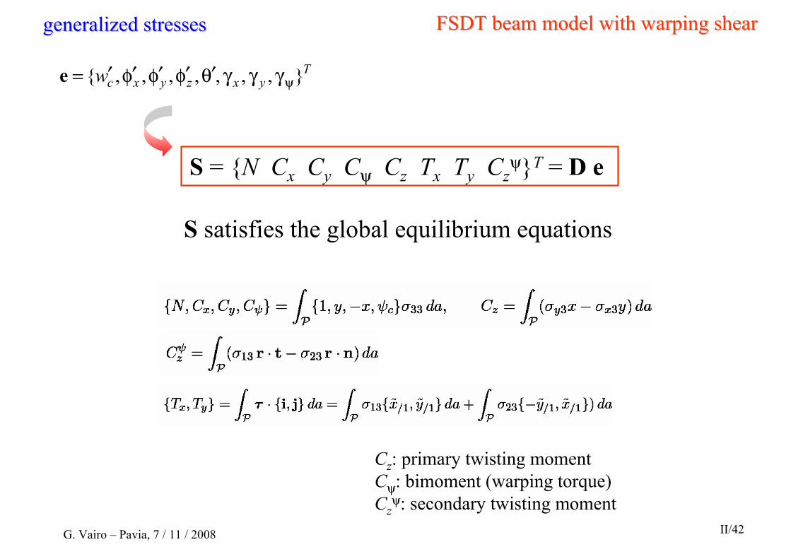
generalized stressesgeneralized stresses FSDT beam model with warping shearFSDT beam model with warping shear
Tyxzyxcw },,,,,,,{ ψγγγθ′φ′φ′φ′′=e
S = {N Cx Cy Cψ Cz Tx Ty Czψ}T = D e
S satisfies the global equilibrium equations
Cz: primary twisting momentCψ: bimoment (warping torque)Cz
ψ: secondary twisting momentG. Vairo – Pavia, 7 / 11 / 2008 II/42
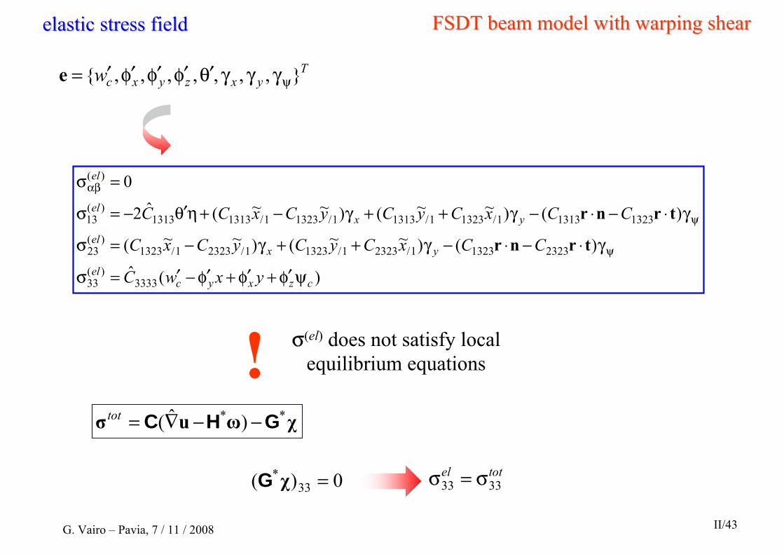
)(ˆ)()~~()~~(
)()~~()~~(ˆ2
0
3333)(
33
232313231/23231/13231/23231/1323)(
23
132313131/13231/13131/13231/13131313)(
13
)(
czxycel
yxel
yxel
el
yxwC
CCxCyCyCxC
CCxCyCyCxCC
ψφ′+φ′+φ′−′=σ
γ⋅−⋅−γ++γ−=σ
γ⋅−⋅−γ++γ−+ηθ′−=σ
=σ
ψ
ψ
αβ
trnr
trnr
σ(el) does not satisfy local equilibrium equations!
χωuσ *tot GHC −−∇= )ˆ( *
totel3333 σ=σ0)( 33 =χ*G
Tyxzyxcw },,,,,,,{ ψγγγθ′φ′φ′φ′′=e
elastic stress fieldelastic stress field FSDT beam model with warping shearFSDT beam model with warping shear
G. Vairo – Pavia, 7 / 11 / 2008 II/43

x (i)
y (j)
O
sso
sl
ξξ
P1i
P2i
n (η)t
internal cross-section
Total shear stresses recoveringTotal shear stresses recoveringalong-z field and boundary equilibrium eqs.
G. Vairo – Pavia, 7 / 11 / 2008 II/44

totel3333 σ=σ
tot23σ
x (i)
y (j)
O
sso
sl
ξξ
P1i
P2i
n (η)t
internal cross-sectionalong-z field and boundary equilibrium eqs.
Total shear stresses recoveringTotal shear stresses recovering
G. Vairo – Pavia, 7 / 11 / 2008 II/44

Other refinements and generalizationsOther refinements and generalizations
G. Vairo – Pavia, 7 / 11 / 2008 II/45

x1
x2
MultiMulti--branch refined assumptionsbranch refined assumptionsAverage over the thickness of total shear strains and elastic shear stresses are piecewise constant functions of the curvilinear abscissa s, i.e. they are assumed to be constant on each branch.
F. Maceri, G. Vairo. Anisotropic thin-walled beam models: a rational deduction from three-dimensional elasticity. to appear on J. of Mechanics of Materials and Structures (2008).
G. Vairo – Pavia, 7 / 11 / 2008 II/46
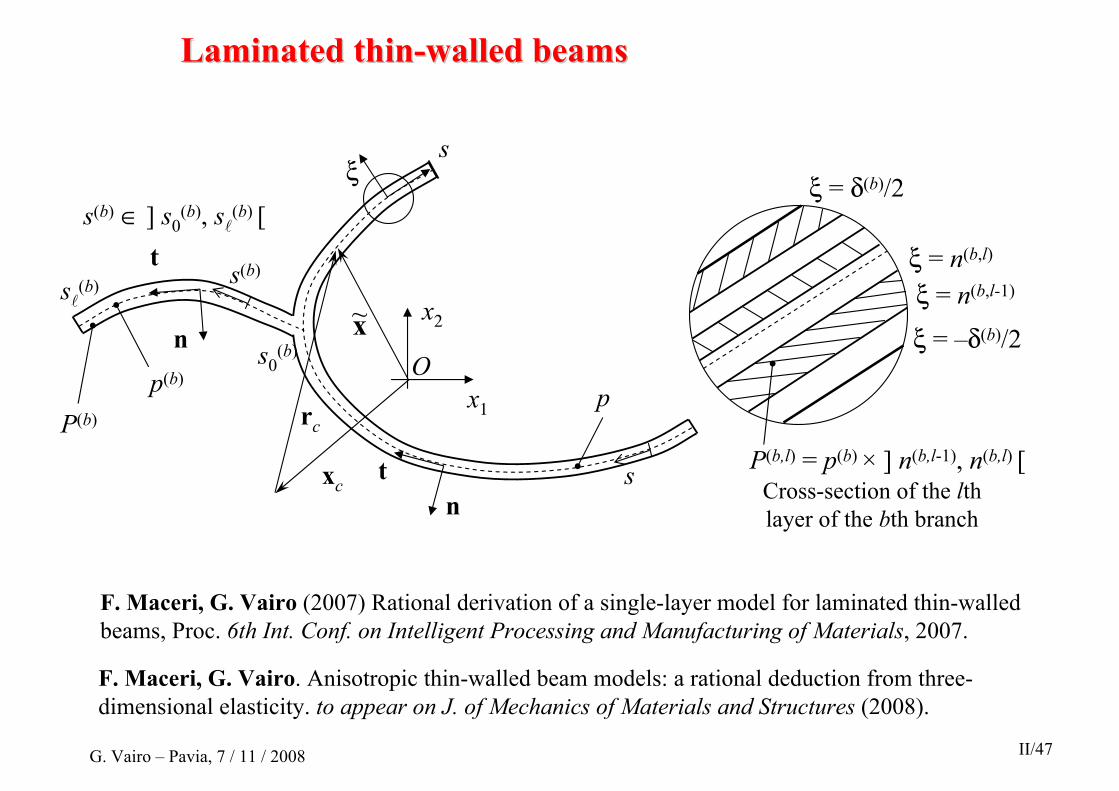
n
ts(b)
sl(b)
s0(b)
P(b)
p(b)
s(b) ∈ ] s0(b), sl(b) [
x1
x2
Ox~
rc
xcn
t s
p
ξs
ξ = n(b,l-1)
ξ = n(b,l)
ξ = –δ(b)/2
ξ = δ(b)/2
Cross-section of the lth layer of the bth branch
P(b,l) = p(b) × ] n(b,l-1), n(b,l) [
Laminated thinLaminated thin--walled beamswalled beams
F. Maceri, G. Vairo. Anisotropic thin-walled beam models: a rational deduction from three-dimensional elasticity. to appear on J. of Mechanics of Materials and Structures (2008).
F. Maceri, G. Vairo (2007) Rational derivation of a single-layer model for laminated thin-walled beams, Proc. 6th Int. Conf. on Intelligent Processing and Manufacturing of Materials, 2007.
G. Vairo – Pavia, 7 / 11 / 2008 II/47
F. Maceri, G. Vairo. Anisotropic thin-walled beam models: a rational deduction from three-dimensional elasticity. to appear on J. of Mechanics of Materials and Structures (2008).
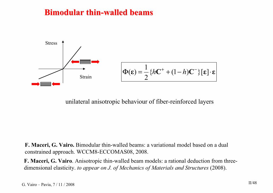
Strain
Stress
εεCCε ⋅−+=Φ −+ ]}[)1({21)( hh
Bimodular thinBimodular thin--walled beamswalled beams
unilateral anisotropic behaviour of fiber-reinforced layers
F. Maceri, G. Vairo. Bimodular thin-walled beams: a variational model based on a dual constrained approach. WCCM8-ECCOMAS08, 2008.
G. Vairo – Pavia, 7 / 11 / 2008 II/48
GiuseppeGiuseppe VairoVairoUniversity of Rome ‘Tor Vergata’Department of Civil Engineeringviale Politecnico, 1 - 00133 Rome – ItalyE-mail: [email protected]
Thank YouThank YouThank You
UniversitUniversitàà degli Studi di Paviadegli Studi di PaviaDipertimento di Meccanica StrutturaleDipertimento di Meccanica Strutturale
7th November, 20087th November, 2008